See discussions, stats, and author profiles for this publication at: https://www.researchgate.net/publication/239731304
FlexParamCurve: R package for flexible fitting
of nonlinear parametric curves
Article in Methods in Ecology and Evolution · December 2012
DOI: 10.1111/j.2041-210X.2012.00231.x
CITATIONS
READS
7
79
4 authors, including:
Andre Chiaradia
Phillip Island Nature Parks
72 PUBLICATIONS 932 CITATIONS
SEE PROFILE
Some of the authors of this publication are also working on these related projects:
Artificial night lights and seabirds: solutions to a fatal attraction View project
All content following this page was uploaded by Andre Chiaradia on 24 April 2015.
The user has requested enhancement of the downloaded file. All in-text references underlined in blue are added to the original document
and are linked to publications on ResearchGate, letting you access and read them immediately.
doi: 10.1111/j.2041-210X.2012.00231.x
Methods in Ecology and Evolution
APPLICATION
FLEXPARAMCURVE: R package for flexible fitting of
nonlinear parametric curves
Stephen A. Oswald1*, Ian C. T. Nisbet2, Andre Chiaradia3 and Jennifer M. Arnold1
1
Division of Science, Pennsylvania State University, Berks Campus, 2080 Tulpehocken Road, PA 19610, USA;
I.C.T. Nisbet & Co., 150 Alder Lane, North Falmouth, MA 02556, USA; and 3Phillip Island Nature Parks, P.O. Box
97, Cowes, Victoria 3922, Australia
2
Summary
1. Nonlinear, parametric curve-fitting provides a framework for understanding diverse ecological
and evolutionary trends (e.g. growth patterns and seasonal cycles). Currently, parametric curve-fitting requires a priori assumptions of curve trajectories, restricting their use for exploratory analyses.
Furthermore, use of analytical techniques [nonlinear least-squares (NLS) and nonlinear mixedeffects models] for complex parametric curves requires efficient choice of starting parameters.
2. We illustrate the new R package FlexParamCurve that automates curve selection and provides
tools to analyse nonmonotonic curve data in NLS and nonlinear mixed-effects models. Examples
include empirical and simulated data sets for the growth of seabird chicks.
3. By automating curve selection and parameterization during curve-fitting, FlexParamCurve
extends current possibilities for parametric analysis in ecological and evolutionary studies.
Key-words: FlexParamCurve, growth analysis, nonmonotonic curve, nonlinear mixed-effects
models, nlsList(), parametric curve-fitting
Introduction
Fitting nonlinear curves has widespread applications in ecological and evolutionary studies, as it can incorporate complex
relationships between variables with greater accuracy than linear regression and greater parsimony than polynomial regression (Pinheiro & Bates 2000; p. 273–277). Although
nonparametric methods are more flexible for large sample
sizes, performance can be unreliable with smaller samples.
Parametric methods are preferred for curve-fitting because of
computational efficiency, low estimator variance and theoretical support (Gedeon, Wong & Harris 1995; p. 552). Choice of
parameters as determined by theory or proposed by hypothesis
facilitates experimental testing and prevents over-fitting
(Kohn, Smith & Chan 2001), as opposed to nonparametric
methods that use purely statistical (not biological) parameters.
Hence, variance in parameter estimation is lower for parametric methods as they are constrained a priori to a specific
function (Gedeon, Wong & Harris 1995, p. 552). Parametric
curve-fitting, therefore, can analyse relatively small data sets
and estimate parameters of biological significance.
Where small data sets exhibit nonmonotonic functional
relationships, monotonic parametric curves (e.g. logistic,
Richards) and nonparametric methods may give inaccurate
*Correspondence author. E-mail:steve.oswald@psu.edu
results. This often arises in ecological studies with few
measurements of each subject (e.g. growth analyses). These
studies have traditionally ignored individual differences and
have not exploited the analytical power of mixed-effects
models (Huin & Prince 2000). Although some ecological
studies now employ more complex parametric models (e.g.
Bunnefeld et al. 2011), selecting a parametric function of
appropriate complexity to accommodate observed trajectories in the data and choosing starting values for its parameters is usually difficult, limiting their general use. Hitherto,
no automated approach exists to perform model selection
for nonmonotonic curves.
Here, we describe a new R (R Development Core Team
2011) package, FlexParamCurve (Oswald 2011), that includes
functions to estimate parameters for nonmonotonic curves
and select the models that best fit datasets. We consider generalized forms of double-logistic, biphasic and bi-logistic curves
providing examples using simulated and empirical data sets.
Description
ECOLOGICAL APPLICATIONS REQUIRING
NONMONOTONIC CURVE-FITTING
Biphasic or nonmonotonic relationships arise in several ecological contexts, including growth in birds, fish, mammals and
2012 The Authors. Methods in Ecology and Evolution 2012 British Ecological Society
2 S. A. Oswald et al.
plants; seasonal migrations or changes in vegetation cover; precipitation-use efficiencies of grasslands and flowering in plants
(published examples cited in Appendix S1 Table S1Æ3).
SELF-STARTING (selfStart) FUNCTIONS
Nonlinear equations generally lack analytical solutions, as they
include products or divisions among their parameters, and
thus are generally solved numerically. Such iterative estimation
approaches require a priori specification of starting values for
all parameters that are refined during the fitting process until
estimation accuracy meets specified convergence criteria. Selection of starting values is often burdensome and, consequently,
self-starting [selfStart()] functions are available for many
curves (Pinheiro & Bates 2000; p.342–346; Ritz & Streibig
2005; Paine et al. 2012).
FlexParamCurve includes a selfStart() function –
SSposnegRichards() – for many nonmonotonic curves.
SSposnegRichards() combines two Richards curves
(Nelder 1962):
y ¼ A=ð½1 þ m expðkðx iÞÞ1=m Þ
0
þ A0 =ð½1 þ m0 expðk0 ðx i0 ÞÞ1=m Þ;
where A, k, i and m are, respectively, the asymptote, rate
parameter, inflection point and shape parameter of the first
Richards curve and A¢, k¢, i¢ and m¢ are the corresponding
parameters for the second curve (parameters described in
Appendix S1 Table S1Æ1). In FlexParamCurve, these parameters are designated Asym, K, Infl, M, RAsym, Rk, Ri and
RM, respectively. Individual Richards curves can model many
sigmoidal forms (e.g. logistic, Gompertz and von Bertalanffy);
the double-Richards curve is equally flexible for nonmonotonic
relationships (Fig. 1).
Parameter redundancy often arises when the equation fitted
is too complex for the data and can lead to estimation
problems. Therefore, FlexParamCurve allows fitting
[SSposnegRichards()] and plotting [posnegRichards.
eqn()] reduced versions of the double-Richards curve by fixing £5 parameters to user-specified values (or means by
default). FlexParamCurve uses this approach because parameters of the Richards curve have empirical biological meaning
for many datasets (e.g. Brisbin et al. 1987). Fixing a parameter
achieves the same numerical advantage (fewer estimable
parameters) but avoids compensatory changes to estimable
parameters that occur when a parameter is dropped. In this way,
by default FlexParamCurve allows the data to suggest the most
parsimonious curve, but also permits users to select appropriate
parameterizations. The default parameter bounds (tested across
diverse datasets) can also be specified by the user.
SSposnegRichards() and posnegRichards.eqn()
use argument modno to specify one of 32 versions of the double-Richards curve (all 16 possible reductions in the second
curve (fixing A¢, k¢, i¢, or m¢) both when m is fixed or estimated;
see Appendix S1 Table S1Æ2 and the SSposnegRichards()
help file). This allows fitting of monotonic curves such as logistic (model 32, m = 1), Gompertz (model 32, m 0) and von
Bertalanffy (model 32, m = )0Æ3), as well as many nonmonotonic forms, for example, double-logistic (model 22,
m = m¢ = 1), double-Gompertz (model 22, m = m¢ 0),
double-von Bertalanffy (model 22, m = m¢ = )0Æ3) and
biphasic growth models (Fig. 1, Appendix S1 Table S1Æ2).
The output from SSposnegRichards() feeds directly
into functions such as nls(), nlsList() and nlme()
(Pinheiro et al. 2007) and is thus compatible with all methods
for these functions [e.g. anova()].
MODEL SELECTION
FlexParamCurve includes functions [pn.mod.compare()
and pn.modselect.step()] to determine the most suitable
Fig. 1. Examples of curves possible in 17 of the 32 model reductions available in FlexParamCurve using the posneg.data data set (see Appendix S2 for code). Models 1–16 estimate all parameters of the first curve and some combination (indicated in panels) of second curve parameters
(A¢, k¢, i¢, m¢), fixing nonestimated parameters to mean values. Models 21–36 (not shown) correspond to 1–16 respectively, with m fixed. Model
32 only estimates A, k and i, allowing 3-parameter curves (logistic curve shown). Examples use default parameter estimates from modpar() for
the first curve (A = 4445, k = 0Æ064, i = 23Æ2, m = 0Æ36) and any fixed parameters but, for illustration, within each panel, lines are plotted for
all possible combinations of nonfixed parameter values (listed in final panel) for estimated second curve parameters.
2012 The Authors. Methods in Ecology and Evolution 2012 British Ecological Society, Methods in Ecology and Evolution
Nonlinear parametric curve-fitting 3
(a)
(b)
Fig. 2. Nonlinear parametric curves fitted to growth data for (a) little
penguins and (b) common terns. Left panel in each row: all data; three
right panels: data for representative individual chicks. Dotted curve:
NLS fit to all data (same curve in each panel); solid curves:
nlsList() fit to data for individuals. nlsList() yields much better fits to data for individuals than the global nonlinear least-squares.
See Appendix S2 for code.
reduction in the double-Richards curve for a data set. These fit
models in nlsList() (Pinheiro et al. 2007), yielding nonlinear least-squares (NLS) fits for each group (e.g. each individual
in a growth analysis). This represents the suitability of a particular curve more robustly than a simple NLS across all groups
(which ignores individual contributions; Fig. 2).
pn.mod.compare() ranks candidate nlsList() models
according to penalized root-mean-square error (pRSE¢):
p
p
ðRr2 =bÞ= n:
where r2 is the estimated variance (square of residual standard
error) for each of the b fitted grouping levels and n is the number of data points fitted. (Rr2 ⁄ b) is root-mean-square error
(RSE) and by default this is divided by n (thus, pRSE¢ represents per level measurement error exponentially discounted by
sample size). This penalizes models that fit only a few groups
and consequently have low RSE (because there is likely less
variation in fit among fewer levels) and allows comparison of
nonnested models (as it uses residual squared error rather than
maximum likelihood). Users can also edit the formulation of
pRSE¢ to match their desired balance between sensitivity and
specificity.
Processing time can be considerable for multiple nlsList()
models with many groups, so pn.mod.compare() and
pn.modselect.step() first evaluate the parsimony of a
fixed shape parameter m. Initially, an extra sum-of-squares
F-test compares the full 8-parameter model (model 1) with a
7-parameter model (model 21) in which m is fixed to the
mean across the data set. If the 8-parameter model provides
a significantly better fit, subsequent reductions explore models in which m is estimated (modno = 2–16). Otherwise,
subsequent evaluations use the same reductions but with m
fixed to the mean across the data set (modno = 22–36) (see
Fig. 1 and Appendix S1 Table S1Æ2).
After assessing the need to estimate m, pn.modselect.
step() uses backwards, step-wise selection of subsequent
nlsList() models. At the next step, four candidate models (each with one of the four-second curve parameters, A¢,
k¢, i¢, m¢, fixed at its mean value) are ranked by pRSE¢ (as
they are not mutually nested) and the highest-ranked
reduction is compared with the general model (1 or 21)
using extra sum-of-squares F-tests (Ritz & Streibig 2009).
This rank-then-test procedure is used at all subsequent
steps.
For additional flexibility, functions extraF() and
extraF.nls() allow users to undertake extra sum-ofsquares F-tests for any two nested nlsList() or nls()
models, respectively.
USING FLEXPARAMCURVE: EXAMPLES FROM AVIAN
GROWTH ANALYSES
The help files for FlexParamCurve provide illustrative examples; see also Figs 1–3 and Appendix S2. Here, we demonstrate the general approach for using FlexParamCurve to
determine the most suitable parametric curve then fit NLS
models or nonlinear mixed-effects models. We use published
data on growth of common terns (Sterna hirundo Linnaeus)
(Nisbet 1975; Nisbet, Wilson & Broad 1978; tern.data)
and little penguins (Eudyptula minor Forster) (Chiaradia &
Nisbet 2006; penguin.data) and a simulated data set for
black-browed albatrosses (Thalassarche melanophrys Temminck; posneg.data see help file). Appendix S3 provides
codes for these examples.
1 Run function modpar() to generate a list of initial
parameter estimates, fitting options and parameter bounds.
This provides information needed to fit [using SSposnegRichards()] and predict [using posnegRichards.eqn()]
and can subsequently be modified manually or with
change.pnparameters(). Calling either model selection
routine automatically calls modpar() if a suitable list is not
supplied.
2 Perform model selection using pn.model.compare()
and pn.modselect.step(). These functions may suggest
different reductions in the double-Richards curve because
pn.model.compare() is more sensitive to curves with low
pRSE¢ and pn.modselect.step() relies on sequential
model reduction. For example, both routines selected a double-Gompertz curve (modno = 22, Table 1, Appendix S1
Table S1Æ2) as the best fit to the posneg.data data set. In
contrast, they each suggested different final models for both
penguin and tern data sets (Table 1). For penguins,
pn.model.compare() selected model (modno) 31, a
4-parameter model including one-second curve parameter
that fitted 90% (122 ⁄ 150) of the individuals in the data set
(Table 1, Fig. 2), rather than the anticipated (Chiaradia &
Nisbet 2006) double-Gompertz curve that required two-second
curve parameters (modno = 34). For terns, pn.model.
compare() selected model (modno) 32, a 3-parameter model
with the shape parameter m fixed at 0Æ72 (mean across the data
set); this fitted 89% (67 ⁄ 75) of the individuals in the data set
2012 The Authors. Methods in Ecology and Evolution 2012 British Ecological Society, Methods in Ecology and Evolution
4 S. A. Oswald et al.
Table 1. Top-ranked models by pn.model.compare() (first subtable) and stepwise selection by pn.modselect.step() (second subtable)
for (a) posneg.data (100 levels), (b) little penguin (150 levels) and (c) common tern (75 levels) data sets. For pn.model.compare() models
are ranked according to minimized, penalized root-mean-square error (pRSE¢) (lowest value in bold), No. of levels fit is the number of groups
(individual chicks) parameterized in nlsList() and No. of params is the number of parameters. For pn.modselect.step(), only the most
general and most reduced models are shown (see Appendix S1 Tables S1Æ4–6 for full output)
(a) posneg.data (black-browed albatross; simulated)
pn.model.compare
modno
pRSE¢
No. of levels fit
RSE
Model d.f.
Residual d.f.
No. of params
22
24
35
79
87
93
12Æ9
14Æ1
19Æ2
474
435
465
553
696
744
6
5
5
0Æ40
0Æ42
0Æ55
pn.modselect.step
Selected
Step
Reduced
General
F
d.f.
P
22
22
6
2
12
22
22
21
323
2Æ56
200, 900
100, 700
<0Æ001
<0Æ001
(b) little penguin
pn.model.compare
modno
pRSE¢
No. of levels fit
RSE
Model d.f.
Residual d.f.
No. of params
31
32
33
1Æ52
1Æ67
2Æ40
122
125
42
64Æ5
72Æ1
59Æ4
488
375
210
1317
1488
400
4
3
4
pn.modselect.step
Selected
Step
Reduced
General
F
d.f.
P
21
21
6
2
12
22
21
21
4Æ85
5Æ82
580, 1630
274, 1324
<0Æ001
<0Æ001
(c) common tern
pn.model.compare
modno
pRSE¢
No. of levels fit
RSE
Model d.f.
Residual d.f.
No. of params
32
33
30
0Æ18
0Æ24
0Æ27
67
32
28
5Æ9
5Æ8
6Æ0
201
160
112
852
448
376
3
5
4
pn.modselect.step
Selected
Step
Reduced
General
F
d.f.
P
12
22
6
3
12
22
22
33
3Æ20
3Æ09
350, 856
544, 1050
<0Æ001
<0Æ001
‘Selected’ indicates the model (modno) preferred from extra F comparisons between the reduced (‘Reduced’) and more general (‘General’)
models tested at this step; extra F statistics are given. Preferred model at Step 6 (bold) is deemed the most suitable. For additional detail,
see Appendix S1.
(Table 1, Fig. 2) and was similar in shape to a logistic curve
(m = 1Æ0).
3 Fit NLS [nls()] or nonlinear mixed-effects models
[nlme()] using the most suitable curve in SSposnegRichards(). Model selection in nls() or nlme() can then
investigate effects of factors, variates or covariates (fixed or
random) on the parameters selected (Pinheiro & Bates 2000; p.
377–409). For example, the penguin data set contains data
from two contrasting years (Chiaradia & Nisbet 2006). When
analysed within a single NLME model (Appendix S3) both
yearly and seasonal differences are evident (Fig. 3).
Conclusion
FlexParamCurve provides ways to fit, plot and compare a multiplicity of monotonic or nonmonotonic parametric curves in
R, using NLS and mixed-effects models. This permits modelling of nonmonotonic relationships with relatively small data
sets, including studies of growth, migration and seasonal vegetation dynamics, both when data are expected to follow a particular nonmonotonic relationship and when the relationship
is as yet unexplored.
2012 The Authors. Methods in Ecology and Evolution 2012 British Ecological Society, Methods in Ecology and Evolution
Nonlinear parametric curve-fitting 5
(a)
(b)
Fig. 3. Comparison of growth of little penguins that hatched early (earliest 16Æ5%; black lines ⁄ open circles) and late (latest 16Æ5%; grey lines ⁄
filled triangles) in (a) 2000 and (b) 2002. Lines are predictions from nlme() using the parametric curve selected by FlexParamCurve.
Acknowledgements
We thank Sinéad English for data and comments during testing, Dieter Menne
for advice on optimization routines and Timothy Paine and one anonymous
reviewer for helpful comments on the manuscript.
References
Brisbin Jr., I.L., Collins, C.T., White, G.C. & McCallum, D.A. (1987) A new
paradigm for the analysis and interpretation of growth data: the shape of
things to come. Auk, 104, 552–554.
Bunnefeld, N., Börger, L., Van Moorter, B., Rolandsen, C.M., Dettki, H.,
Solberg, E.J. & Ericsson, G. (2011) A model-driven approach to quantify
migration patterns: individual, regional and yearly differences. Journal of
Animal Ecology, 80, 466–476.
Chiaradia, A. & Nisbet, I.C.T. (2006) Plasticity in parental provisioning and
chick growth in Little Penguins Eudyptula minor in years of high and low
breeding success. Ardea, 94, 257–270.
Gedeon, T.D., Wong, P.M. & Harris, D. (1995) Balancing bias and variance:
network topology and pattern set reduction techniques. From Natural to
Artificial Neural Computation: International Workshop on Artificial Neural
Networks (eds J. Mira & F. Sandoval), pp. 551–558. Springer-Verlag, Berlin.
Huin, N. & Prince, P.A. (2000) Chick growth in albatrosses: curve fitting with a
twist. Journal of Avian Biology, 31, 418–425.
Kohn, R., Smith, M. & Chan, D. (2001) Nonparametric regression using linear
combinations of basis functions. Statistics and Computing, 11, 313–322.
Nelder, J.A. (1962) Note: an alternative form of a generalized logistic equation.
Biometrics, 18, 614–616.
Nisbet, I.C.T. (1975) Selective effects of predation in a tern colony. Condor, 77,
221–226.
Nisbet, I.C.T., Wilson, K.J. & Broad, W.A. (1978) Common Terns raise young
after death of their mates. Condor, 80, 106–109.
Oswald, S.A. (2011) FlexParamCurve: Tools to Fit Flexible Parametric Curves.
R Foundation for Statistical Computing, Vienna, Austria. Available at:
http://cran.r-project.org/web/packages/FlexParamCurve/index.html
(accessed 6 December 2011).
Paine, C.E.T., Marthews, T.R., Vogt, D.R., Purves, D., Rees, M., Hector, A. &
Turnbull, L.A. (2012) How to fit nonlinear plant growth models and calculate growth rates: an update for ecologists. Methods in Ecology and Evolution, 3, 245–256.
Pinheiro, J. & Bates, D. (2000) Mixed-Effects Models in S and S-Plus. SpringerVerlag, Berlin.
Pinheiro, J., Bates, D.M., DebRoy, S. & Sarkar, D. (2007) nlme: Linear and
Nonlinear Mixed Effects Models. R Foundation for Statistical Computing,
Vienna, Austria. Available at: http://cran.r-project.org/web/packages/nlme/
index.html (accessed 6 December 2011).
R Development Core Team (2011) R: A Language and Environment for
Statistical Computing. R Foundation for Statistical Computing, Vienna,
Austria. Available at: http://www.R-project.org (accessed 6 December
2011).
Ritz, C. & Streibig, J.C. (2005) Bioassay analysis using R. Journal of Statistical
Software, 12, 1–22.
Ritz, C. & Streibig, J.C. (2009) Nonlinear Regression with R. Use R!. Springer,
New York, NY, USA.
Received 30 December 2011; accepted 15 May 2012
Handling Editor: Mark Rees
Supporting Information
Additional Supporting Information may be found in the online
version of this article.
Appendix S1. Parameter descriptions, the 32 formulations of parametric curves possible within FlexParamCurve and examples of their
application.
Appendix S2. R scripts for all figures.
Appendix S3. R scripts for worked examples.
As a service to our authors and readers, this journal provides supporting information supplied by the authors. Such materials may be
re-organized for online delivery, but are not copy-edited or typeset.
Technical support issues arising from supporting information (other
than missing files) should be addressed to the authors.
2012 The Authors. Methods in Ecology and Evolution 2012 British Ecological Society, Methods in Ecology and Evolution
Keep reading this paper — and 50 million others — with a free Academia account
Used by leading Academics

Billie J. Swalla
University of Washington

Jorge Urbán
Universidad Autonoma de Baja California Sur (UABCS)
Jeffrey Schwartz
University of Pittsburgh

Yasha Hartberg
Texas A&M University