Progress In Electromagnetics Research M, Vol. 76, 75–89, 2018 Rapidly Adaptive CFAR Detection in Antenna Arrays Anatolii A. Kononov* Abstract—This paper addresses the problem of target detection in adaptive arrays in situations where only a small number of training samples is available. Within the framework of two-stage adaptive detection paradigm, the paper proposes a class of rapidly adaptive CFAR (Constant False Alarm Rate) detection algorithms, which are referred to as joint loaded persymmetric-Toeplitz adaptive matched filter (JLPT-AMF) detectors. A JLPT-AMF detector combines, using a joint detection rule, individual scalar CFAR decisions from two rapidly adaptive two-stage (TS) detectors: a TS TAMF detector and a TS LPAMF detector. The former is based on a TMI filter, which is an adaptive array filter employing a Toeplitz covariance matrix (CM) estimate inversion. The latter is based on an adaptive LPMI filter that uses diagonally loaded persymmetric CM estimate inversion. The proposed class of adaptive detectors may incorporate any rapidly adaptive TS TAMF and TS LPAMF detectors, which, in turn, may employ any scalar CFAR detection algorithms that satisfy an earlier derived linearity condition. The two-stage adaptive processing structure of the JLPT-AMF detectors ensures the CFAR property independently of the antenna array dimension M , the interference CM, and the number of training samples NCME to be used for estimating this CM. Moreover, the rapidly adaptive JLPT-AMF detectors exhibit highly reliable detection performances, which are robust to the angular separation between the sources, even when NCME is about m/2 ∼ m, m is the number of interference sources. The robustness is analytically proven and verified with statistical simulations. For several representative scenarios when the interference CM has m dominant eigenvalues, comparative performance analysis for the proposed rapidly adaptive detectors is provided using Monte-Carlo simulations. Abbreviations and Acronyms ACE Adaptive Coherence Estimator LPMI Loaded Persymmetric Matrix (Estimate) Inversion AMF Adaptive Matched Filter LR Low Rank BAD Basic Adaptive Detector LSMI Loaded Sample Matrix Inversion BD Benchmark Detector ROC Receiver Operating Characteristic CFAR Constant False Alarm Rate SCM Sample Covariance Matrix CM Covariance Matrix SNR Signal-to-Noise Ratio DOA Direction of Arrival SRL Statistical Resolution Limit GLRT Generalized Likelihood Ratio Test TAMF Toeplitz (Matrix Estimate Inversion) AMF INR Interference-to-Noise Ratio TCME Toeplitz Covariance Matrix Estimation Joint Loaded Persymmetric-Toeplitz TMI Toeplitz Matrix (Estimate) Inversion JLPT-AMF (Matrix Estimates Inversion) AMF LAMF Loaded (Sample Matrix Inversion) AMF TS Two-Stage LPAMF Loaded Persymmetric (Matrix Estimate ULA Uniform Linear Array Inversion) AMF Received 24 September 2018, Accepted 12 November 2018, Scheduled 27 November 2018 * Corresponding author: Anatolii A. Kononov (kaa50ua@gmail.com). The author is with the Research Center, STX Engine, 288, Guseong-ro, Giheung-gu, Yongin-si, Gyeonggi-do 16914, Republic of Korea. 76 Kononov 1. INTRODUCTION For adaptive array filters, the minimum number of training samples N3 dB required to ensure the average signal-to-noise ratio (SNR) loss within 3 dB relative to the optimal Wiener filter is generally accepted as the convergence measure of effectiveness [1–3]. It is well-known that the 3 dB average SNR loss for adaptive array filters that employ the sample covariance matrix (SCM) estimator   R̂ = N −1 XN XH (1) N can be achieved if the training sample size N meets the condition N ≥ N3 dB ≈ 2M . In Eq. (1) above, we assume that the N -sample training data matrix XN ∈ CM ×N is composed of N independent and identically distributed (i.i.d.) samples xi ∼ CN (M, 0, R), i = 1, 2, . . . , N , having an M -variate complex-valued zero-mean circular Gaussian distribution with common covariance matrix R; the superscript H denotes the Hermitian transposition. In most adaptive detector radar applications, the available training sample size N is substantially limited [2, 3], namely N ≪ M . Thus, achieving highest convergence rate — minimizing N3 dB — is one of the major problems in designing adaptive detectors. Efficient solutions to this problem take advantage of certain favorable properties of the disturbance CM resulting from physical nature in the interference and array geometry. For instance, one of the physically adequate models of the exact interference CM R at the array output is given as a sum of the full rank covariance due to the white thermal noise of power σo2 and a CM of a low-rank m (m ≪ M ) resulting from the m powerful external interference sources. As is well known, for this kind of low-rank (LR) structure models, the eigenspectrum of R comprises m dominant eigenvalues (sorted in descending order) followed by M -m equal minimum eigenvalues λ1 ≥ λ2 ≥ . . . ≥ λm ≫ λm+1 = . . . = λM = σo2 = po . (2) N3 dB ≈ 2m, (3) N3 dB ≈ m (4) Many adaptive detection techniques exist that rely on the LR structure property of the matrix R, see, e.g., [2–4] and references therein. The essential advantage of these techniques is that N3 dB is independent of the array dimension M , and is given by which is a significant convergence performance improvement over well-known basic adaptive detectors (BADs) [2]: the generalized likelihood ratio test (GLRT), the adaptive matched filter (AMF), and the adaptive coherence estimator (ACE), all of which require N ≥ N3 dB ≈ 2M . Also, note that the diagonally loaded sample matrix inversion (LSMI) filter [2], employing the diagonally loaded SCM of the R̂(β) = R̂ + (βpo )I form, with β being the real-valued loading factor, behaves as an LR method, i.e., N3 dB for the LSMI filter is also given by Eq. (3). This behavior is analytically proven in [5, 6] for the “cliff-like” (LR structure matrix R) scenarios of Eq. (2). In terms of linear algebra, a set of m linearly independent vectors (basis) is needed to specify the signal subspace of the exact interference CM R. Therefore, the lower bound for N3 dB is assumed to be m [2]. However, as first proven in [5], the statistically justified lower bound for N3 dB in “cliff-like” interference scenarios of Eq. (2) is given by Eq. (3) if the adaptive filter exploits only the LR structure of R. In this paper, we assume an adaptive antenna that employs a uniform linear array (ULA) of M omnidirectional sensors with inter-sensor spacing d/λ = 0.5, where λ is the wavelength determined by a common center frequency of m external far-field sources that radiate continuous narrow-band plane waves simultaneously impinging upon the array. Thus, more efficient covariance estimators should incorporate, in addition to the LR structure property, information on the structure of the exact CM R due to the ULA geometry. As shown in [7], exploiting the persymmetry of the matrix R in addition to the LR structure property, leads to essential performance improvement; the required sample support is instead of 2m when only the LR structure property is employed. Formula (4) can be explained by considering a specific symmetry of the eigenvectors of Hermitian persymmetric matrices. As has been shown in [8, 9], the upper M /2 entries in each eigenvector are equal to the reversed complex conjugate lower M /2 entries. Hence, when the exact interference CM is Progress In Electromagnetics Research M, Vol. 76, 2018 77 persymmetric, the statistical information contained in the training samples is used to estimate only M free real variables, which are the unbound real and imaginary parts of entries in the m signal subspace (dominant) eigenvectors. This number of free variables is less by a factor of two than that when only the LR structure property is employed. Recall, if the estimator employs only the LR structure, then N3 dB ≈ 2m. Thus, if the persymmetry is employed in addition to the LR structure property, other conditions being equal, one can expect the required training sample size to be halved, i.e., N3 dB ≈ m. All Toeplitz matrices are persymmetric; hence, their eigenvectors also possess the specific symmetry property described above. Moreover, the eigenvectors of Hermitian Toeplitz matrices possess another kind of symmetry such that the imaginary part in any eigenvector is just its reversed real part, with, perhaps, a sign change [9]. Thus, in the case of the Toeplitz CM, the number of free real variables to be estimated is reduced by a factor of two in addition to the reduction resulting from the persymmetry. In this case, one can, therefore, assume that the statistically justified N3 dB can be evaluated as N3 dB ≈ m/2. (5) The adaptive Toeplitz covariance matrix estimate inversion (TMI) filters based on the Toeplitz CM estimation (TCME) algorithm proposed in [10] exhibit a superfast convergence rate in terms of the 3 dB average SNR loss in the low-rank covariance scenarios when the true CM of the interference R has a “cliff-like” eigenspectrum of Eq. (2). The TMI filters require m/2 training samples to achieve the 3 dB average SNR loss, while the diagonally loaded persymmetric matrix inversion (LPMI) filters [10] and the conventional diagonally loaded sample matrix inversion (LSMI) filters [2, 14] require m and 2m samples, respectively. However, the TMI filters can achieve a very high convergence rate if the angular separation between sources does not too closely approach a certain statistical resolution limit (SRL) that can be evaluated based on the results in [11]. As demonstrated in [10] for the MUSIC-based TMI filter (when the TCME algorithm employs MUSIC as a DOA estimator), the convergence performance of the TMI filter may degrade due to an unacceptable drop in output SNR when the angular separation between sources is near the SRL that has been defined in [10] as 0.5FRL , (6) SRL = (SNRarr )1/4 where FRL = 2π/M is the standard Fourier resolution limit, and SNRarr = 4 · M · SNRelt is the array SNR with SNRelt being the element-level SNR. Using other DOA estimators in the TCME algorithm, such as Root-MUSIC [12] or ESPRIT [13], can make TMI filters less sensitive to the small angular separation between sources [10]. This approach, however, does not provide a reliable remedy because performance breakdown resides in all known DOA estimators. The abovementioned BADs (GRLT, AMF, and ACE) possess the strict CFAR property (if N ≥ M ), however, they require a considerable number of training samples N to ensure the reliable detection performance [2, 14]. This is because the BADs use a generic maximum-likelihood SCM estimator in Eq. (1) that ignores any a priori information on the structure of the exact CM R. Indeed, as was earlier found out in [15, p. 125] the generic SCM requires some number of secondary training samples that exceeds the dimension of the antenna array “by a significant factor if noise estimation is not to cause a serious loss in performance” and, therefore, “the requirements on the number of secondaries may be extremely large”. It should be noted that detectors employing the TMI filters proposed in [10] are not strictly CFAR detectors; loss of the CFAR property is the price paid for achieving superfast convergence. We will further show that a practically efficient solution to the CFAR loss problem in adaptive detectors with superfast TMI filters exists in the framework of an approach proposed by Kalson [16]. He made an important observation that the BADs use only simple mean level cell averaging and the sample matrix inversion method of array vector synthesis and the same data set is used for both cell averaging and weight vector synthesis. In [16], Kalson introduced a new class of adaptive algorithms based on the concept of two-stage adaptive processing. This concept assumes that the training (secondary) data are used to design adaptive array filters that provide efficient interference suppression (first stage), while the subsequent adaptive detection exploits conventional scalar CFAR methods over a set of adaptively processed (at the first stage) primary range/Doppler cells that are presented by data statistically 78 Kononov independent of the training samples. Thus, the algorithms in this new class use two statistically independent data sets for weight vector synthesis and CFAR detection. This approach gives one much greater flexibility because any method of weight vector synthesis and a variety of scalar CFAR methods (not only mean level cell averaging) may be used. A sufficient condition for the second-stage scalar CFAR processing was derived in [16]. The only restriction this condition places upon a function to be used in computing scalar CFAR detection threshold is that it obeys the simple linearity property, which is easy to satisfy in practice. A practical example of the two-stage adaptive processing is an adaptive antenna array system where adaptive array filter is used for jamming suppression only, and the final target detection is carried out at the output of coherent Doppler processing applied for clutter rejection [2, 14]. In this case, some amount of training range and Doppler cells that are free of clutter and targets (perhaps those collected over time intervals free of radar transmissions) is used to estimate the interference CM. The resultant adaptive array filter is then applied across the operationally significant (primary) range/Doppler cells to suppress the interference. Final target detection is realized after coherent Doppler processing in the clutter/interfering targets background by using scalar CFAR techniques. An essential feature of such a two-stage processing structure is that the sample data train the adaptive array filter for externalnoise suppression, but they do not represent the entire background interference against which targets of interest must be finally discriminated. Thus, the CFAR property in adaptive array detection can be achieved within the framework of the two-stage adaptive processing paradigm. As noted in [2, 14], this approach appears to be the only feasible adaptive detection option for applications, like that one mentioned above, with different interference properties over the secondary and primary data. A similar approach may also be considered as an alternative to the basic adaptive detectors even for the homogeneous training conditions that are the standard model in designing conventional one-stage CFAR detectors. In the case of homogeneous training conditions, if N is fixed, a set of N i.i.d. training samples allocated for any single primary range cell is divided into two subsets of the NCME and the NCFAR samples [2, 14]. The former is used in estimating the interference CM to design an adaptive filter, while the latter is used in computing the scalar CFAR threshold for target detection. For non-homogeneous training conditions, however, NCFAR is the number of primary cells used for adaptive scalar CFAR detection; NCME and NCFAR cannot be traded-off against each other since both correspond to data sets containing different interferences. As follows from Kalson’s theory [16], an essential feature of two-stage adaptive detection structures is that the required number of samples for adaptive CFAR control NCFAR is independent of the array dimension. For a sufficiently large array dimension M , therefore, any adaptive array filter requiring significantly smaller training sample support to achieve efficient interference suppression than that required for filters employing the generic SCM estimator (N3 dB ≈ 2M ), will lead to more efficient two-stage adaptive detectors than any of the BADs. Hence, the superfast TMI filter introduced in [10] is the filter of choice for use in two-stage adaptive detectors. However, the TMI filters achieve a very high convergence rate (N3 dB ≈ m/2) only if the angular separation between the interference sources is not too close to the SRL given by (6). It should be noted that two-stage detection structure guarantees only strict CFAR control; it does not eliminate detection performance degradation due to a possible output SNR drop in TMI filters in scenarios with closely spaced interference sources. The present paper discusses the construction of a new class of rapidly adaptive CFAR detection algorithms, which are referred to as joint loaded persymmetric-Toeplitz adaptive matched filter (JLPTAMF) detectors. A JLPT-AMF detector combines, using a joint detection rule, individual scalar CFAR decisions from two rapidly adaptive two-stage (TS) detectors: a TS TAMF detector and a TS LPAMF detector. The former is based on a TMI filter, which is an adaptive array filter employing a Toeplitz covariance matrix estimate inversion. The latter contains an adaptive LPMI filter that uses diagonally loaded persymmetric CM estimate inversion. The proposed class may incorporate any rapidly adaptive TS TAMF and TS LPAMF detectors, which, in turn, may employ any scalar CFAR detection algorithms that satisfy a simple linearity condition derived in [16]. The two-stage adaptive processing structure of the JLPT-AMF detectors ensures the CFAR property independently of the antenna array dimension M , the interference CM R, and the number of Progress In Electromagnetics Research M, Vol. 76, 2018 79 training samples NCME to be used for estimating this CM. The joint detection rule, which combines individual CFAR decisions from the TS TAMF and TS LPAMF detectors, guarantees the detection performances of the JLPT-AMF detectors are robust to the angular separation between the interference sources. Moreover, the JLPT-AMF detectors exhibit highly reliable and robust detection performances, even when NCME is on the order of m/2 ∼ m. This robustness is analytically proven and verified with statistical simulations. In Section 2, we discuss a necessary condition of reliable adaptive detection by analyzing the ratio of the number of real variables in all the complex-valued entries of training vector samples to the total number of free real variables in the dominant (signal subspace) eigenvectors of the exact covariance matrix R of the total noise. We analyze this ratio depending on a priori information on the structure of R incorporated into the CM estimator. Section 3 describes the adaptive detectors under study. This Section starts from the TS LAMF detectors earlier introduced in [16] and substantially investigated in [2, 14], we use it as a reference detector in the comparative performance analysis; next, Section presents the TS LPAMF and TS TAMF detectors, and then the new JLPT-AMF detector based upon them. In Section 3, we also prove the robustness of the JLPT-AMF detectors to the angular separation between interference sources. In Section 4, for several representative scenarios when the exact CM at the ULA output has m dominant eigenvalues with m ≤ M/2, we provide a comparative performance analysis for the proposed JLPT-AMF detectors and other two-stage adaptive detectors under study using statistical simulations. Section 5 summarizes the main results. 2. CONDITION OF RELIABLE ADAPTIVE DETECTION Table 1 below summarizes the ratio Q of the total number of real variables QTDS (all real and imaginary parts) contained in the complex-valued entries of training data samples, to the total number of free real variables QFRV contained in the complex-valued entries of all the dominant eigenvectors of the exact CM R depending on a priori information about R incorporated into the CM estimator. In Table 1, the quantity QTDS is represented as QTDS = N3 dB × Q1TS , where Q1TS is the number of real and imaginary parts in one training vector sample. The quantity QFRV is represented as QFRV = NDEV × Q1EV , where NDEV is the number of the dominant eigenvectors of R, and Q1EV is the number of free real variables in each dominant eigenvector. Table 1. Number of real training variables per one free real variable depending on a priori information on structure of exact CM. Structure of Exact CM General Low-rank (LR) LR + Persymmetry LR + Toeplitz Total number of real variables in training data set, QTDS 2M × 2M 2m × 2M m × 2M m/2 × 2M Total number of free real variables, QFRV M × 2M m × 2M m×M m × M/2 Q = QTDS /QFRV 2 2 2 2 Analysis of the Q = QTDS /QFRV ratio in Table 1 leads to the conclusion that the following necessary condition of reliable adaptive detection is valid (at least for Gaussian interference); Q must meet the condition Q > 2 to ensure reliable adaptive detection; in other words, the ratio of the total number of real variables in a training data set to the total number of free real variables in the dominant eigenvectors of the exact covariance matrix must exceed 2. This fundamental condition has been verified for general and for low-rank structures of the true CM; rigorous proofs, in terms of the probability density functions for the SNR at the output of adaptive filters, are given in [1] and [5, 6], respectively. The two remaining cases in Table 1 have not yet been rigorously proven; however, numerous Monte-Carlo simulations confirm these cases. 80 Kononov 3. ADAPTIVE DETECTORS UNDER STUDY 3.1. Two-Stage LAMF Detector The two-stage loaded adaptive matched filter (TS LAMF) detector consists of the LSMI filter and the scalar CFAR detector [2, 14]. The TS LAMF detector computes the statistic ηLAMF and then compares it against the scalar CFAR threshold constant h to derive the decision regarding the presence of a target as given below by Eq. (7) in case of homogeneous training conditions (environment) H H1 |wLSMI y|2 = η ≷ h, (7) LAMF H R̂CFAR wLSMI wLSMI H0 where the CFAR threshold constant h is precomputed for a given probability of false alarm PFA ; H0 and H1 respectively stand for the null hypothesis (no target is present) and the alternative hypothesis (target is present). In Eq. (7) above, the M -by-1 complex vector y denotes the primary cell under test (CUT), and the weight vector of the LSMI filter is given by wLSMI = R̂CME (β)−1 st , (8) jπu jπ2u jπ(M −1)u T where the M -by-1 complex vector st = s(θt ) = aW ◦ [1, e , e , ..., e ] , u = sin θt is H the normalized (st st = 1) array-signal steering vector for a target from a given direction θt with aW = [a1 a2 ... aM ]T being a unit norm weighting vector (the symbol ◦ stands for the Hadamard product); the matrix R̂CME (β) is computed as R̂CME (β) = R̂CME + (β p̂o )I, (9) where R̂CME is the sample covariance matrix R̂CME = 1 NCME N CME xk xH k, (10) k=1 which is computed using NCME i.i.d. training samples xk , k = 1, 2, . . . , NCME , that share the common interference CM R with the CUT data vector y. The parameters β and p̂o are respectively, the realvalued loading factor and the thermal noise power estimate, and I denotes the identity matrix of order M . As recommended in [2], the loading factor should be selected using the condition 1 < β ≤ 3. In Eq. (7) above, the matrix R̂CFAR is also computed (in the case of the homogeneous environment) using the estimator in Eq. (1) as N  1 (11) xk xH R̂CFAR = k, NCFAR k=NCME +1 where the vectors xk , k = NCME + 1, ..., N, are the i.i.d. complex training samples, which also share the common interference CM R with y; these vectors represent the NCFAR = N − NCME primary range/Doppler cells of interest in the vicinity of the individual CUT associated with the vector y. To derive the scalar CFAR form for the TS LAMF detector, we substitute Eq. (11) into the denominator in Eq. (7). After simple algebra we get H R̂CFAR wLSMI wLSMI = N CFAR 1 NCFAR zq , (12) q=1 where the scalar CFAR reference samples zq are given by H zq = |wLSMI xq+NCME |2 , q = 1, 2, ..., NCFAR . (13) H 2 Denoting the numerator in Eq. (7) as z = |wLSMI y| and using Eq. (13) leads to the scalar cell averaging (CA) CFAR representation for the LSMI detector in Eq. (7) H1 1 H0 NCFAR z≷h N CFAR q=1 H1 ′ zq or z ≷ h H0 N CFAR zq . (14) q=1 where using the precomputed modified CFAR constant h′ = h/NCFAR excludes dividing by NCFAR . Progress In Electromagnetics Research M, Vol. 76, 2018 81 3.2. Two-Stage LPAMF Detector The two-stage diagonally loaded persymmetric adaptive matched filter (TS LPAMF) detector consists of the LPMI filter [10] and the scalar CFAR detector. The TS LPAMF detector computes the statistic ηLPAMF and compares it against the scalar CFAR threshold constant h to make the detection decision H |wLPMI yP |2 H1 H wLPMI R̂PCFAR wLPMI = ηLPAMF ≷ h, (15) H0 where the M -by-1 vector yP = UP y is the transformed CUT data vector y with UP being the unitary matrix given by   1 I2 J2 , (16) UP = √ 2 jI2 −jJ2 where I2 and J2 , respectively, are the M /2-by-M /2 identity and exchange matrix (without the loss of generality, we consider only the even M case); the weight vector of the LPMI filter is given by wLPMI = R̂RPCME (β)−1 sPt (17) with the vector sPt being defined as sPt = UP st and the matrix R̂RPCME (β) being computed as R̂RPCME (β) = R̂RPCME + (β p̂o )I, (18) where the symmetric matrix R̂RPCME representing the persymmetric CM estimate of the exact CM R is computed as [10, 17] R̂RPCME = Re(UP R̂CME UH (19) P ). In Eq. (15) above, the matrix R̂PCFAR is given by R̂PCFAR = UP R̂CFAR UH P. Introducing the transformed weight vector vLPMI = form of the TS LPAMF detector in Eq. (15) H |vLPMI y|2 H vLPMI R̂CFAR vLPMI (20) UH P wLPMI leads to the following simplified H1 = ηLPAMF ≷ h. (21) H0 It is straightforward to derive the following scalar CFAR forms of the TS LPAMF detector in Eq. (21) N N CFAR CFAR H1 H1 1 ′ zPq , (22) zPq or zP ≷ h zP ≷ h H0 H0 NCFAR q=1 q=1 H where zP = |vLPMI y|2 and the scalar CFAR reference samples zPq are given by H zPq = |vLPMI xq+NCME |2 , q = 1, 2, ..., NCFAR . (23) Using the LPMI weight vector in the form given by Eq. (17) is reasonable in case of a stand-alone implementation of the TS LPAMF detector. When we use this detector as part of a JLPT-AMF detector (see Subsection 3.4 below), a computationally efficient version of the LPMI weight vector is available. This version allows significantly reducing the computational complexity of the LPMI filter since it does not require the matrix inversion operation as in Eq. (17). Indeed, the TCME algorithm [10] includes computing the eigendecomposition of the symmetric matrix R̂RPCME given by Eq. (19). This eigendecomposition consists of the eigenvalues λ̂k , which are ordered as |λ̂1 | ≥ |λ̂2 | ≥ ... ≥ |λ̂M |, and their correspondingly ordered eigenvectors êk , k = 1, 2, ..., M . Then, the matrix R̂RPCME in (19) can be presented as R̂RPCME = ÊΛ̂ÊH , where Ê = [ê1 ê2 ... êM ], and Λ̂ = diag[|λ̂1 | , |λ̂2 | , ... , |λ̂M |]. (24) 82 Kononov Substituting Eq. (24) into Eq. (18) we have R̂RPCME (β) = ÊΛ̂ÊH + (β p̂o )I. (25) Applying the matrix inversion lemma to Eq. (25) readily yields the closed-form expression of the inverse of the matrix R̂RPCME (β) R̂RPCME (β)−1 = (β p̂o )−1 [I − ÊΦ̂ÊH ], (26) where Φ̂ is a diagonal matrix with diagonal entries (Φ̂)ii = |λ̂i |/(|λ̂i | + β p̂o ), for i = 1, 2, ..., M . Using Eq. (26), the weight vector wLPMI (17) and, correspondingly the vector vLPMI in Eq. (21), is computed with no matrix inversion operation as (27) wLPMI = [I − ÊΦ̂ÊH ]sPt , −1 where the term (β p̂o ) is excluded since multiplying the weight vector by an arbitrary constant does not change the signal-to-noise ratio (SNR) and the detection statistic ηLPAMF in Eqs. (15) and (21). 3.3. Two-Stage TAMF Detector The two-stage Toeplitz adaptive matched filter (TS TAMF) detector consists of the TMI filter [10] and the scalar CFAR detector. The TS TAMF detector computes the statistic ηTAMF and then compares it against the scalar CFAR threshold constant h to make the detection decision H y |2 H1 |wTMI T = η ≷ h, (28) TAMF H R̂ wTMI H0 TCFAR wTMI where the M -by-1 vector yT = UT y is the transformed CUT data vector y with UT being the unitary matrix given by 1 (29) UT = √ [I − jJ] , 2 where I and J respectively, is the M -by-M identity and exchange matrix; the weight vector of the TMI filter is given by wTMI = R̂−1 RTCME sTt with the vector sTt being defined as sTt = UT st ; the symmetric matrix R̂RTCME is computed as [10] R̂RTCME = Re(UT R̂TCME UH T ), (30) where the complex matrix R̂TCME is the Toeplitz CM estimate being computed using the TCME algorithm [10] with NCME training samples xk , k = 1, 2, ..., NCME ; the matrix R̂TCFAR is computed as R̂TCFAR = UT R̂CFAR UH (31) T. H Introducing the transformed weight vector vTMI = UT wTMI yields the following simplified form of the TS TAMF detector in Eq. (28) H y|2 H1 |vTMI = ηTAMF ≷ h. (32) H vTMI R̂CFAR vTMI H0 The scalar CFAR forms of the TS TAMF detector in Eq. (32) are given by H1 1 H0 NCFAR zT ≷ h N CFAR q=1 H1 ′ zTq or zT ≷ h H0 N CFAR zTq , (33) q=1 H y|2 and the scalar CFAR reference samples z where zT = |vTMI Tq are given by H zTq = |vTMI xq+NCME |2 , q = 1, 2, ..., NCFAR . (34) It should be noted that using the scalar CFAR forms in Eqs. (14), (22), and (33) is especially beneficial in nonhomogeneous environments when the vectors xk , k = NCME + 1, ..., N (corresponding to a set of some primary Range/Doppler cells) to be used in scalar CFAR thresholding are not identically distributed due to the clutter edges and/or interfering targets; though these vectors are independent and include the same signals of m interference sources, which are present in the CUT vector y. Having obtained the scalar CFAR reference samples given by Eqs. (13), (23) and (34) allows using new adaptive CFAR approaches [18, 19] in severely nonhomogeneous environments to provide significant improvements in both, false alarm regulation and detection performance. Progress In Electromagnetics Research M, Vol. 76, 2018 83 3.4. JLPT-AMF Detector We define the joint loaded persymmetric-Toeplitz adaptive matched filter (JLPT-AMF) detector as an adaptive detection algorithm that combines the scalar CFAR decisions from the TS LPAMF detector in Eq. (21) or (22) and the TS TAMF detector in Eq. (32) or (33) using the following rule if ηLPAMF ≥ hi or ηTAMF ≥ hi then H1 is true, otherwise H0 is true, (35) P (A) = Pr{ηLPAMF ≥ hi |H1 } and P (B) = Pr{ηTAMF ≥ hi |H1 }. (36) PD = P (A) + P (B) − P (AB) = P (A) + P (B) − P (B)P (A|B), (37) where hi is the individual CFAR threshold associated with a given individual probability of false alarm PFAi . It follows from Eq. (35) that the decision strategy adopted in the JLPT-AMF detector is to declare that the hypothesis H1 is true whenever at least one of the individual detectors decides that H1 be true. Theorem. The detection probability of detector (35) exceeds the maximum of the individual detection probabilities. Proof. Let A denote the event ηLPAMF ≥ hi and B denote the event ηTAMF ≥ hi . Then, assuming that the hypothesis H1 is true, the individual probabilities of detection for the TS LPAMF detector and the TS TAMF detector are, respectively, Suppose, for instance, that P (A) ≥ P (B). Since the events A and B are not disjoint, the overall detection probability PD for the JLPT-AMF detector in Eq. (35) can be written as where P (B) − P (B)P (A|B) = P (B)[1 − P (A|B)] > 0. Thus, PD > P (A). This completes the proof. This theorem above establishes the self-adjustment property of the JLPT-AMF detector; for the detector in Eq. (35), the overall detection probability PD is automatically maintained at a level such that the PD value always exceeds the maximum of the individual probabilities. For this reason, if the angular separation between sources is far enough from the SRL given by Eq. (6), the overall PD value of the detector in Eq. (35) is maintained at some level exceeding the individual detection probability of the TS TAMF detector. If the TS TAMF detector performance should degrade due to the presence of closely spaced sources, the detector in Eq. (35) will automatically maintain the overall detection probability PD at some level that exceeds the individual detection probability of the TS LPAMF detector in Eq. (21). As shown in [10], the latter is not sensitive to the angular separation between the interference sources. The detector in Eq. (35) robustness to the angular separation between sources is ensured thereby. Note that detector in Eq. (35) also increases the overall probability of false alarm PFA , i.e., PFA > PFAi . The upper bound for PFA follows from the inequality PFA ≤ 2PFAi that can easily be proven assuming the hypothesis H0 is true. 4. ANALYSIS OF DETECTION PERFORMANCE In the detection performance analysis, we consider a scenario with a Swerling I target embedded in the interference with covariance matrix R that meets the condition in Eq. (2). We model the primary vector sample y as  xo ∼ CN (M, 0, R) for hypothesis H0 , (38) y= xo + ast , a ∼ CN (0, pt ) for hypothesis H1 where xo ∈ CM ×1 is the observed interference plus receiver noise — only complex data vector and a represents the target complex amplitude fluctuations which average power is pt . In our analysis, we compare the receiver operating characteristics (ROCs) of the JLPT-AMF detector in Eq. (35) with that of other two-stage adaptive detectors described in Section 3. This analysis assumes homogenous training conditions when the full set of N = 2M independent and identically distributed secondary training samples allocated for any single primary cell is divided into two subsets of size NCME (for interference CM estimation) and NCFAR (for CFAR thresholding), NCME +NCFAR = N . All the TS TAMF and JLPT-AMF detectors analyzed in this section use the Root MUSIC-based TMI filters which employ the exemplary Toeplitz CM estimation algorithm from [10] with all the parameter settings specified in [10]. 84 Kononov For performance comparison, we also use the following benchmark detectors. Benchmark detector 1 (BD1): BD1 is an optimal or clairvoyant detector achieving ultimate −1 detection performance. This detector comprises the optimal Wiener filter wopt = R−1 st /(sH t R st ), which is followed by the decision rule H1 |yH R−1 st |2 ≷ h. = η BD1 −1 sH H0 t R st The well-known expression [20, p. 108] describes the ROC curve of the detector in Eq. (39)  PD = exp −| ln PFA |/(1 + q 2 ) , (39) (40) where the output SNR of the optimal Wiener filter is −1 q 2 = pt sH t R st . (41) The ultimate performance of Eq. (40) corresponds to NCME → ∞ and NCFAR → ∞. Benchmark detector 2 (BD2): BD2, a two-stage detector, comprises optimal Wiener filter and scalar cell averaging (CA) CFAR |yH R−1 st |2 −1 R̂R−1 s sH t t R H1 = ηBD2 ≷ h, (42) H0 Consequently, the detector in Eq. (42) uses all N training samples for adaptive CFAR detection (NCFAR = N ). The ROC of the detector in Eq. (42) is given by [20, p. 599]  −N h′ PD = 1 + , (43) 1 + q2 −1/N where the modified CA CFAR constant h′ = h/N = PFA − 1. Equation (43) corresponds to the case NCME → ∞ and NCFAR = N . In all examples herein, we use a ULA of M = 12 sensors, a Hamming weighted steering vector st tuned to θt = 0 (providing a quiescent array pattern with −39 dB sidelobes), and the real loading factor β = 2 for both the LSMI and the LPMI filters. The noise power estimate p̂o in Eqs. (9) and (25) for the LSMI and the LPMI filter, respectively, is taken from the TCME algorithm [10] that generates the Toeplitz CM estimate R̂TCME in Eq. (30) for the TMI filter. The number of training samples for estimating covariance matrix NCME = 5 and for estimating the adaptive scalar CFAR threshold NCFAR = 19 (NCME + NCFAR = N = 2M = 24). Then, for the overall probability of false alarm −1/N PFA = 10−4 and NCFAR = 19, the CA CFAR constant h = NCFAR (PFA CFAR − 1) = 11.8517580; similarly, for the individual probability of false alarm PFAi = 0.671141 × 10−4 (this value of PFAi ensures the given overall PFA for the JPLT-AMF detector) and NCFAR = 19 we have hi = 12.5061245. 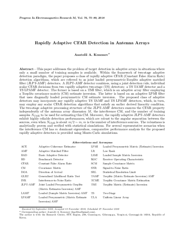Figure 1 compares the ROC of the JLPT-AMF detector with that of the TS LAMF detector, and with that of the TS LPAMF and the TS TAMF detectors in Scenario B (we use the scenario designations from [10]) Scenario B : m = 4, u = [−0.8, −0.4, 0.2, 0.5], INR (dB) = [20, 20, 20, 20], where the vector u = [sin θk , k = 1, 2, . . . , m] and the vector INR (dB) = [10 lg(pk /po ), k = 1, 2, . . . , m] respectively, represents the DOAs θk , k = 1, 2, . . . , m and the individual interference-to-noise ratios (INRs) for external sources with powers pk , k = 1, 2, . . . , m. In Scenario B, the interference sources are well-separated in the angular coordinate, and we also assume that both the thermal noise power po = σo2 and the number of sources m are not known. By the well-separated sources, we understand the interference sources with such the smallest angular separation between them that is not too close to the SRL computed from Eq. (6). In Fig. 1, the curves labeled “BD1” and “BD2” represent the ROCs for the corresponding benchmark detectors in the same scenario. One of the ROC curves for the BD2 is calculated for PFA = 10−4 using Eq. (43) with h′ = 0.4677993 and another is estimated using the Importance Sampling (IS) technique employing a so-called g-method [21]. We developed two modified versions of the g-method: for estimating the probability of false alarm in case of arbitrary interference CM R, Progress In Electromagnetics Research M, Vol. 76, 2018 85 1 0.9 0.8 ULA: d/ = 0.5; M = 12 Hamming weighting Beam Steering Angle = 0 0.7 Scenario B: m = 4; u = [-0.8, -0.4, 0.2, 0.5]; INR(dB) = [20, 20, 20, 20] 0.6 DOA Estimator for TMI filter: Root MUSIC BD1 for PFA Eq. (40) NCME = 5; NCFAR = 19 BD2 for PFA Eq. (43) Number of sources is not known TS TAMF for PFA (IS) BD2 for PFA (IS) 0.5 0.4 0.3 JLPT-AMF for PFA (MC) Noise power is not known TS TAMF for PFAi (IS) TS LPAMF for PFA (IS) TS LPAMF for PFAi (IS) 0.2 TS LAMF for PFA (IS) 0.1 0 IS = Estimated using Importance Sampling MC = Estimated using conventional Monte-Carlo 5 10 15 SNR (dB) 20 25 30 Figure 1. ROCs for the adaptive detectors under study in Scenario B. and for estimating the detection performance for the target model specified by Eq. (38). The perfect match between these two ROC curves (i.e., between the analytic and estimated results) validates the high accuracy of the modified versions of the g-method: for Nis = 64, 000 independent statistical trials, the average relative standard deviation error is ∼ 2% in estimating the probability of false alarm PFA and ∼ 0.1% in estimating the detection probability PD (0.3≤ PD ≤ 0.99). Similarly, the ROC curves for the TS LAMF, the TS LPAMF, and the TS TAMF detectors are also computed using the modified versions of the g-method with Nis = 64, 000. Fig. 1 plots two ROC curves at PFA = 10−4 and PFAi = 0.671141 × 10−4 for each of the TS LPAMF and the TS TAMF detectors. Unfortunately, the g-method cannot be used for the JLPT-AMF detector; instead, we use the conventional Monte-Carlo (MC) technique with Nis = 107 to verify PFA and with Nis = 64, 000 to calculate the ROC curves. Figure 1 shows that the JLPT-AMF detector exhibits superior detection performance in a scenario with well-separated (in angular dimension) interference sources: for PD = 0.5, the SNR gain relative to the TS LPAMF and the TS LAMF detectors is 2.3 dB and 5.4 dB, respectively, while the SNR loss relative to the unrealizable BD2 is just 0.5 dB. Figure 2 plots the ROCs for all the detectors being studied, and the ROCs for the BD1 and BD2 detectors in Scenario D1 : m = 3, u = [−0.4, 0.0, sin(SRL)], INR (dB) = [20, 20, 20], in which the smallest angular separation between sources is SRL = 1.8021085◦ (0.0314527 rad) for the SNRelt = max(INR2 , INR3 ) = 20 dB; both the noise power po and the number of sources m are assumed to be unknown. Fig. 2 confirms the self-adjustment property of the JLPT-AMF detector. Indeed, the ROC curve for the JLPT-AMF detector goes above that for the TS TAMF detector; the latter represents the maximum of the two individual detection probabilities associated, respectively, with the TS LPAMF and the TS TAMF detectors at the specified PFAi . Figure 3 shows the ROC curves in Scenario D2 : m = 3, u = [−0.4, 0.0, sin(∆θ)], INR (dB) = [28, 20, 30] that is unfavorable for the TS TAMF detector. In this scenario, the smallest angular separation ∆θ between sources is equal to SRL = 1.0134◦ (0.0176872 rad) for the SNRelt = max(INR2 , INR3 ) = 30 dB, and it is assumed that both the noise power po and the number of sources m are not known. As can be seen in Fig. 3, although the TS TAMF detector suffers essential performance degradation, for the JLPT-AMF detector, the ROC curve goes above that of the TS LPAMF detector at PFAi = 0.671141 × 10−4 and slightly above that at PFA = 10−4 . Fig. 3 confirms that the JLPT-AMF detector is robust. Kononov Probability of Detection 86 Probability of Detection Figure 2. ROCs for the adaptive detectors under study in Scenario D1 . Figure 3. ROCs for the adaptive detectors under study in Scenario D2 . For Scenario D2 , Fig. 4 plots the curves that represent the probability of detection as a function of the relative angular separation ∆θ/SRL between the second and third sources for the fixed NCME = 5 (NCFAR = 19) and target SNR = 25 dB; the parameter ∆θ represents the angular separation between the second and third sources. From Fig. 4, the TS TAMF detector collapses for 0.8SRL ≤ ∆θ ≤ 2.7SRL, while for the JLPT-AMF detector, the PD curve is above that of the TS LPAMF detector independently of the angular separation ∆θ. Fig. 4 also confirms the robustness of the proposed JLPT-AMF detector. It is noteworthy that when the number of sources m is known (rank-constrained scenarios), the performance of the Root MUSIC-based TMI filter is robust to the angular separation between the 87 Probability of Detection Progress In Electromagnetics Research M, Vol. 76, 2018 Figure 4. Estimated probability of detection versus ∆θ/SRL for the adaptive detectors under study in Scenario D2 . Figure 5. ROCs for the adaptive detectors under study in Scenario D2 (the number of sources m is known). sources [10]. In Scenario D2 , under the condition that the number of sources m is known and the noise power po is not known, Figs. 5 and 6 present the plots similar to those shown in Figs. 3 and 4, respectively. Thus, Figs. 5 and 6 confirm that in case of a rank-constrained scenario, i.e., when m is known, not only the JLPT-AMF detector but also the TS TAMF detector (each of them employs the Root MUSIC-based TMI filter) is fundamentally robust to the angular separation. 88 Kononov Figure 6. Estimated probability of detection versus ∆θ/SRL for the adaptive detectors under study in Scenario D2 (the number of sources m is known). 5. CONCLUSIONS We have presented a class of rapidly adaptive CFAR detection algorithms for antenna arrays in situations with a limited amount of available training data. These detection algorithms are referred to as joint loaded persymmetric-Toeplitz adaptive matched filter (JLPT-AMF) detectors. A JLPT-AMF detector combines, using a joint detection rule, individual scalar CFAR decisions from rapidly adaptive two-stage TAMF and LPAMF detectors. The proposed class may incorporate any rapidly adaptive two-stage TAMF and LPAMF detectors, which, in turn, may employ any scalar CFAR algorithms that satisfy the simple linearity condition derived in [16]. An essential feature of the JLPT-AMF detectors is that they provide the exact CFAR property independently of the antenna array dimension, the interference covariance matrix, and the number of training samples to be used for estimating this matrix. Moreover, these new rapidly adaptive CFAR detectors outperform other known fast two-stage adaptive CFAR detectors. The JLPT-AMF detectors exhibit highly reliable detection performances, which are robust to the small angular separation between the sources, even when the training sample size to be used for estimating the interference covariance matrix is about m/2 ∼ m (m is the number of interference sources). This robustness is analytically proven and verified with statistical simulations. It should also be noted that in case of rank-constrained scenarios (i.e., when m is known), both the TS TAMF detector and the JLPT-AMF detector are fundamentally robust to the angular separation if they employ the Root MUSIC-based TMI filter. It is noteworthy that the rapidly adaptive JLPT-AMF detectors admit adaptive scalar CFAR thresholding using the scalar reference samples computed from the corresponding adaptively processed primary vector samples. Having obtained the scalar reference samples, new scalar CFAR approaches, recently introduced in [18, 19], can be used in implementing JLPT-AMF detectors. In severely nonhomogeneous environments, these approaches provide significant improvements in both false alarm regulation and detection performance relative to other scalar CFAR techniques. Finally, we have shown that the fundamental necessary condition of reliable adaptive detection is determined by the ratio of the total number of real variables in a training data set to the total number of free real variables in the dominant eigenvectors of the exact covariance matrix; this ratio must exceed 2 to ensure reliable adaptive detection. Progress In Electromagnetics Research M, Vol. 76, 2018 89 REFERENCES 1. Reed, I. S., J. D. Mallett, and L. E. Brennan, “Rapid convergence rate in adaptive arrays,” IEEE Transactions on Aerospace and Electronic Systems, Vol. 10, No. 6, 853–863, November 1974. 2. Maio, A. D. and M. S. Greco, Modern Radar Detection Theory, Chapter 6, 239–257, Y. I. Abramovich and B. A. Johnson, SciTech Publishing, Edison, NJ, 2016. 3. Steiner, M. and K. Gerlach, “Fast converging adaptive processor for a structured covariance matrix,” IEEE Transactions on Aerospace and Electronic Systems, Vol. 36, No. 4, 1115–1126, October 2000. 4. Peckham, C. D., A. M. Haimovich, T. F. Ayoub, et al., “Reduced-rank STAP performance analysis,” IEEE Transactions on Aerospace and Electronic Systems, Vol. 36, No. 2, 664–676, April 2000. 5. Cheremisin, O., “Efficiency of adaptive algorithms with regularized sample covariance matrix,” Radio Eng. Electron. Phys., Vol. 27, No. 10, 69–77, 1982. 6. Gierull, C. H., “Statistical analysis of the eigenvector projection method for adaptive spatial filtering of interference,” IEE Proc. — Radar, Sonar Navig., Vol. 144, No. 2, 57–63, April 1997. 7. Ginolhac, G., P. Forster, F. Pascal, and J. P. Ovarlez, “Exploiting persymmetry for low-rank space time adaptive processing,” Signal Processing, Vol. 97, No. 4, 242–251, Elsevier, 2014. 8. Goldstein, M. J., “Reduction of the eigenproblem for Hermitian persymmetric matrices,” Math. Computation, Vol. 28, No. 125, 237–238, January 1974. 9. Wilkes, D. M., S. D. Morgera, F. Noor, and M. H. Hayes, III, “A Hermitian Toeplitz matrix is unitarily similar to a real Toeplitz-plus-Hankel matrix,” IEEE Trans. SP, Vol. 39, No. 9, 2146–2148, September 1991. 10. Kononov, A. A., C. H. Choi, and D. H. Kim, “Superfast convergence rate in adaptive arrays,” Proc. Int. Conf. Radar, Brisbane, Australia, August 27–30, 2018. 11. Smith, S. T., “Statistical resolution limits and the complexified Cramér-Rao bound,” IEEE Trans. SP, Vol. 53, No. 5, 1602, May 2005. 12. Barabell, A. J., “Improving the resolution performance of eigenstructure-based direction-finding algorithms,” Proc. ICASSP, 336–339, Boston, MA, 1983. 13. Roy, R. and T. Kailath, “ESPRIT-estimation of signal parameters via rotational invariance techniques,” IEEE Trans. on ASSP, Vol. 37, No. 7, 984–995, July 1989. 14. Abramovich, Y. I., B. A. Johnson, and N. K. Spencer, “Sample-deficient adaptive detection: Adaptive scalar thresholding versus CFAR detector performance,” IEEE Transactions on Aerospace and Electronic Systems, Vol. 46, No. 1, 32–46, January 2010. 15. Kelly, E., “An adaptive detection algorithm,” IEEE Transactions on Aerospace and Electronic Systems, Vol. 22, No. 1, 115–127, March 1986. 16. Kalson, S., “Adaptive array CFAR detection,” IEEE Transactions on Aerospace and Electronic Systems, Vol. 31, No. 2, 534–542, April 1995. 17. Pailloux, G., P. Forster, J. P. Ovarlez, and F. Pascal, “Persymmetric adaptive radar detectors,” IEEE Transactions on Aerospace and Electronic Systems, Vol. 47, No. 4, 2376–2390, October 2011. 18. Kononov, A. A., J.-H. Kim, J.-K. Kim, and G. Kim, “A new class of adaptive CFAR methods for nonhomogeneous environments,” Progress In Electromagnetics Research B, Vol. 64, 145–170, 2015. 19. Kononov, A. A. and J. Kim, “Efficient elimination of multiple-time-around detections in pulseDoppler radar systems,” Progress In Electromagnetics Research B, Vol. 71, 55–76, 2016. 20. Richards, M. A., J. A. Scheer, and W. A. Holm, Principles of Modern Radar, Vol. I, Basic Principles, SciTech Publishing, Raleigh, NC, 2010. 21. Srinivasan, R. and M. Rangaswamy, “Importance sampling for characterizing STAP detectors,” IEEE Transactions on Aerospace and Electronic Systems, Vol. 43, No. 1, 273–285, January 2007.