GUIDELINE FOR PREPARATION Proceedings of the 10th International Ship Stability Workshop Probabilistic Assessment of Ship Stability Based on the Concept of Critical Wave Groups Nikos Themelis & Kostas J. Spyrou National Technical University of Athens, Greece ABSTRACT A versatile methodology for the probabilistic assessment of ship stability is discussed through application to a post-panamax containership, assumed to operate on a North Atlantic route in days of unfavourable weather. Some technical implementation issues are discussed concerning the effect of initial conditions on the calculated probability figures, on the basis of a first-principles approach. KEYWORDS Ship; stability; probability; wave group; dynamics; containership; initial conditions INTRODUCTION The development of an all-purpose probabilistic methodology of ship stability assessment is receiving recently significant international attention, perhaps due to the central role that it is destined to play in an anticipated risk-based framework of ship design and operation. A physics-based methodology for probabilistic stability assessment has been put forward recently by the authors (Themelis & Spyrou 2007). Calculation effort targets the probability to encounter specific wave groups that incite roll dynamic responses of unacceptable intensity, condition that is loosely described in the current context as practical manifestation of “instability”. The present paper is basically a sequel along this line of research and its purpose is dual: firstly, to demonstrate an application of the methodology for the “short-term” assessment of a post panamax containership on a specific voyage from Hamburg to New York. Days of “bad weather” had been identified in advance on the basis of a hindcast study. Three modes of instability, namely beam-seas resonance, parametric rolling and pure-loss of stability, are addressed. Secondly, to undertake a theoretical investigation concerning the quantitative effect produced by a probabilistic consideration of initial conditions, upon the specification of the critical wave groups, and eventually on the overall probability figures. The matter is a theoretically demanding one and here only a preliminary (yet systematic) study will be presented. THE CONTAINERSHIP AND THE ROUTE Basic data concerning the assessed containership are shown in Table 1. Unfortunately, no information of her bilge keels was available, so a bare hull was only considered. The selected route between Hamburg and New York is a rather popular one for containerships, although here the unusual choice of going over the Shetlands has been made. 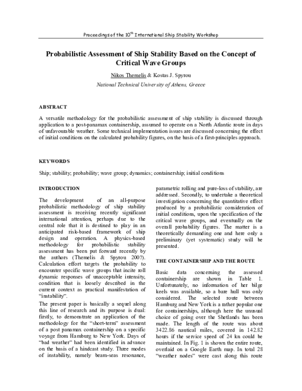The length of the route was about 3422.86 nautical miles, covered in 142.82 hours if the service speed of 24 kn could be maintained. In Fig. 1 is shown the entire route, overlaid on a Google Earth map. In total 28 “weather nodes” were cast along this route GUIDELINE FOR PREPARATION Proceedings of the 10th International Ship Stability Workshop (Fig. 2). Their density was decided by ensuring that wave characteristics, in terms of significant wave height H S and peak period TP , do not change significantly while the ship is still inside the influence area of any particular node. Table 1: Ship data LBP (m) 264.4 m Cb 0.600 B (m) 40 T0 (s) 39.12 D (m) 24.3 KG(m) 18,79 Td (m) 13.97 GM (m) 0.61 VS (kn) 24 TEU 5048 The variation of H S , TP and of the mean wave direction ΘM , in the vicinity of the defined route, are presented in Figs. 3 to 5. The percentage of the ship’s scaled time of exposure to beam, head and following seas per node had then to be worked out on the basis of ship heading (as defined by the route) and the distribution of mean direction of the local wave field around each node, weighted by the time spent in its area of influence (Fig. 6). H S [m] 12 10 8 6 4 2 0 1 3 5 7 9 11 13 15 17 19 21 23 25 27 weather node Fig. 3 : Variation of significant wave height along the route. Fig. 1 : Hamburg - New York route. TP 17.5 [s] 15.5 13.5 11.5 9.5 7.5 5.5 1 3 5 7 9 11 13 15 17 19 21 23 25 27 17 19 21 23 25 27 weather node Fig. 4 : Variation of peak period. Fig. 2 : Part of route showing weather nodes and their areas of influence. Wave hindcast data for the North Atlantic referring to the period between 1990 and 1999 has been consulted (Behrens 2006). As the intention was to perform a “short-term” assessment, the data was searched in order to find specific days of bad weather at places near to the ship’s route. It was found that waves of significant height exceeding 10 m should have been realised in some part of the route, in the period between 13/01/1991 and 18/01/1991. ΘΜ [deg.] 340 300 260 220 180 140 1 3 5 7 9 11 13 15 weather node Fig. 5 : Variation of mean wave direction (00 waves coming from North, 900 East). GUIDELINE FOR PREPARATION Proceedings of the 10th International Ship Stability Workshop Shift- of-cargo threshold Percentage of exposure 7.00% 6.00% 5.00% Following-Seas 4.00% Head-Seas 3.00% 2.00% Beam-Seas 1.00% 0.00% 1 3 5 7 9 11 13 15 17 19 21 -1.00% weather node Fig. 6 : Exposure to beam, head and following seas. NORMS OF UNSAFE RESPONSE These norms are defined respectively as: a critical roll angle for the ship and a critical acceleration for the cargo. 23 This was identified by the critical transverse acceleration that could result in damage of the containers’ lashings. The acceleration due to rolling motion has been estimated for tiers of 4, 5 and 6 TEUs, placed on the deck. The relevant calculations have been carried out according to the Cargo Securing Manual (DNV 2002). Specifically, the sufficiency of lashings’ in terms of transverse sliding and tipping of the tier has been checked. The lashing arrangement is shown in Fig. 8. In Table 2 have been collected the principal parameters that enter into the calculations. The mass per unit of TEUs is consistent with the loading condition for the specified metacentric height. “Capsize” threshold To determine a roll angle as threshold of “capsize” the principle of the weather criterion was adopted. The critical angle should then be the minor of: the angle of vanishing stability ϕc = 520 ; the flooding angle ϕ f and the prescribed value ϕa = 500 . The flooding angle was assumed to correspond to the least transverse inclination (with submerged volume preserved) at which the highest point of a hatch coaming is immersed. According to the drawings, hatch coamings rise 1.7 m above the deck. A rendered view of the hull (with some key deck structures) inclined to that angle is shown schematically in Fig. 7. From hydrostatic calculations it should be ϕ f = 350 . CG z d lashing 2 lashing 1 deck b Fig. 8 : TEUs in a tier and their lashing arrangement. 2 α y [m/s ] 10 8 Transverse Tipping 6 4 Transverse Sliding 2 4 5 number of TEUs in tiers Fig. 7 : Critical heel angle for immersion of hatch coaming. Fig. 9 : Critical transverse accelerations for sliding and tipping for three cases of cargo stowage. 6 GUIDELINE FOR PREPARATION Proceedings of the 10th International Ship Stability Workshop Table 2 : Cargo and lashings characteristics Total number of TEUs: 5048 Total weight of TEUs: 51100t Cargo mass: (4/5/6 TEUs in tier) m = 40.49/ 50.61/ 60.74 t Most severe position of trailer: y=18.28 m z=24.3 m (from base line) Centre of gravity above deck: zd = 4.88/ 6.10/ 7.32 m lever-arm of tipping: b = 1.219 m Coefficient of friction: Steel – steel: µ = 0.1 Lashing arrangement: 2 chains with MSL = 100 kN on each side, symmetrical vertical securing angle per lashing: 43°/60° The most critical condition was identified to correspond to transverse sliding for a tier of 6 TEUs (Fig.9). The specific value of this critical acceleration was calculated as a y = 4.02 m/s 2 . critical wave groups, referring respectively to ship and trailer responses. We have to remind that no bilge keels have been considered Nonlinear Froude-Krylov force has been included in the calculation. Fig. 10 : 3D plots mesh generation of containership by SWAN2. CRITICAL WAVES Critical wave groups have been specified for the following types of instability: a) beam-sea resonance, b) parametric rolling in longitudinal seas; and c) pure-loss of stability. Their characteristics were found from numerical simulations, using the well-known panel code SWAN2 (2002). Fig. 10 shows characteristic 3D plots mesh generation of the containership, as obtained with SWAN2. φ (deg) 40 30 20 10 0 0 10 20 30 40 50 60 70 -10 -20 -30 -40 Beam-seas resonance To determine the critical combinations of wave height, period and group run length that could generate exceedence of a stability norm, deterministic numerical simulations have been carried out. The ship was assumed with no initial rolling. The practical range of wave periods that could be realised in the specific sea region has been scanned. Fig. 11 presents a rolling response to one of the identified as critical wave groups. Fig. 12 and Fig. 13 present the key characteristics of identified t (s) Fig. 11 : Response in beam waves for T=15.5 s and H =9.6 m. Head-seas parametric rolling For the assumed speed of VS = 24 kn the ship could be prone to head-seas parametric rolling. Specifically, the principal mode of parametric instability can be realised when the wavelength obtains values likes those shown in Fig. 14. The required wavelengths are extremely long. An uncertain initial roll disturbance range was GUIDELINE FOR PREPARATION Proceedings of the 10th International Ship Stability Workshop considered in order to realize growth of roll amplitude. Up to a sequence of 8 wave encounters has been examined; because having more waves in a group is of truly negligible probability when the waves are high. The characteristics of critical wave groups were determined from repetitive numerical simulations, taking record whenever roll growth up to the critical norm was realised, within the allowed number of wave encounters. An example is shown in Fig. 15. The variation of critical height and run length in the vicinity of exact principal resonance can be seen in Fig. 16. 4.50 4.00 3.50 λ/L 3.00 2.50 0.7 0.8 0.9 1 1.1 1.2 α Fig. 14 : Critical wavelengths for head-seas parametric rolling (principal resonance). φ (deg) 40 30 20 18 10 0 0 16 10 20 30 40 50 60 70 80 90 100 -10 n=2 -20 14 -30 H cr (m) -40 t (s) n=3 12 Fig. 15 : Parametric roll growth in head waves 80 % off principal resonance and for H=14 m. n=4 n =5 10 n=6 20 8 9.5 12.5 15.5 18.5 T(s) α= 0.7 15 Fig. 12 : Critical wave groups of containership with 0.8 Hcr (m) reference to the limiting roll angle (ship). 0.9 1 10 12 5 3 4 5 6 7 8 7 8 n (number of waves) 11 n=2 20 10 Hcr (m) n =3 9 15 n=4 8 Hcr (m) 1.2 α= 1 n=5 10 7 6 9.5 n =6 1.1 5 12.5 15.5 T(s) 18.5 3 4 5 6 n (number of waves) Fig. 13 : Critical wave groups of containership for the Fig. 16 : Required wave height for reaching the critical roll limiting transverse acceleration (cargo). angle form an initial roll disturbance “around” 4.50. GUIDELINE FOR PREPARATION Proceedings of the 10th International Ship Stability Workshop Pure – loss As the panel code is not suitable for use at very low frequencies of encounter, an analytical criterion of pure loss of stability was used. The key idea exploited was that the critical fluctuation of GZ could be identified on the basis of the following condition: the time of experiencing negative restoring in the vicinity of a crest should be, at least, equal to the time that is necessary for developing capsizal inclination, assuming an initial roll disturbance. In Figure 17 is shown the calculated critical fluctuation of GM hcr for various values of λ L . The respective critical wave heights were calculated taking into account the restoring variation on the waves using Maxsurf. However their values were extremely high and so had very small probability to be met. 3.60 3.40 3.20 3.00 φο=0-3 deg. φο=3-6 deg. hcr 2.80 2.60 2.40 2.20 2.00 0.85 0.9 0.95 λ/L 1 1.05 1.1 Fig. 17 : Critical values of h for pure-loss-of-stability. CALCULATION OF PROBABILITIES For the background theory of wave groups and a brief description of the joint and marginal probability density functions that are necessary for the calculations one may consult for example Themelis and Spyrou (2007). Briefly, the sequence of waves that forms the wave group is treated as a Markov chain. The theory is based on Kimura (1980) as improved later by Battjes & Van Vledder (1984). The necessary probability calculations exploit spectral information of the wave field; i.e. there is no need of using direct time-series results. The JONSWAP spectrum was assumed in order to expedite the calculation procedure In the presentation of the results we have introduced the concept of “critical time ratio”. Rather than using probability figures that refer essentially to number of wave encounters irrespectively of their periods, we considered as more meaningful to convert probabilities of encountering wave groups to the scaled time ratio of experiencing these wave groups according to the formula ti = ti T = Pi i where ttot Tm Pi is the calculated probability of a wave group i having wave period around the value Ti ; ttot is the duration of the part of the voyage inside the rectangle of the considered node and Tm is the mean spectral period associated with the same node. The obtained results presents the scaled critical time per node for each type of instability along the route, thus one can easily deduce which type of instability is more likely to occur at any specific stage of the journey, hence providing useful information for weather routeing. In Fig. 18 are overlaid the three obtained “critical time ratio” curves, for the ship and her cargo respectively. In Table 3 are presented the total probabilities and critical time ratios for the complete voyage taking into account the percentage of exposure to beam, head and following seas. It could be perhaps enlightening if we presented an example of the calculation of the probability of “instability” with reference to a specific part of the route. Take for example node 5 whereabouts the time spent is 3.83 hr. The sea state is characterized by H S = 7.6m and TP = 16.4 s . The probability of critical waves for that node and for cargo shifting is 7.23 x 10-5. For the assumed speed, the mean encounter wave period is 12.66 s and the number of waves encountered by the ship in one hour should be 13777(s)/12.66(s)=1089. Hence the probability of instability for this time of exposure should be 7.88% which is quite a high value (one recalls here of course GUIDELINE FOR PREPARATION Proceedings of the 10th International Ship Stability Workshop that the bilge-keels were not considered, which would reduce this number substantially). ti cargo 1.0E+00 beam seas resonance 1.0E-10 head seas parametric rolling 1.0E-20 1.0E-30 1.0E-40 1 3 5 7 9 11 13 15 17 19 21 23 nodes ti ship Setting up the problem and methodology 1.0E+00 T beam seas resonance head seas parametric rolling 1.0E-20 pure loss 1.0E-40 1.0E-60 1 3 5 7 9 11 13 15 17 19 21 nodes Fig. 18 : Collective view of “critical time ratio” diagrams for cargo (upper) and for ship (lower). Table 3 Summed probability of instability and associated “critical time” Ship: ( ϕ > 35 ) Cargo: ( a y > 4 m/s2) 0 deduced probability figure; in which case, one should better treat as probabilistic quantity the initial state, integrating it thereafter with the subsequent calculation of the probability of exceedence of the stability norm. Apparently, the probability to be found at a certain neighbourhood of the system’s state space is connected to the weather. Better understanding of the role of initial conditions in the calculation of the probability of instability would be very desirable. Pi ti 3.33E-04 3.95E-05 9.38E-04 1.11E-04 23 As any given state z 0 =  z (τ 0 ) , z& (τ 0 ) of a dynamical system can be regarded as initial condition for any state zi that belongs to z0’s later time evolution, a system’s safe basin could be realistically taken as the appropriate continuum of initial conditions that should be targeted for probabilistic treatment. Given a ship and a sea state, one could sensibly assume that each infinitesimal subregion dA within it could be associated with a probability of being “visited” at the moment when the wave group excitation is applied. Let us define the encounter of wave group with the condition of being at the trough of the first wave. EFFECT OF INITIAL CONDITIONS As becomes obvious, a significant element of the current methodology is the identification of the complete set of critical wave groups by numerical or analytical techniques. Whichever route is selected however, an initial state of the system should be assumed because the assessment is based on transient response. The simplest scenario of course is to assume that the ship is initially upright with zero roll velocity and in vertical equilibrium condition when approached by the wave group. This idea has some background from ship roll dynamics investigations (Rainey and Thomson 1991). However, a question could be raised whether this assumption is really critical for the Fig. 19 : Phase-plane trajectories and basin boundary of conservative nonlinear oscillator. Lines of constant potential-plus-kinematic energy of a simple freely oscillating Hamiltonian nonlinear oscillator are shown in Fig. 19. As known, these are approximately cyclic at small energy levels (i.e. linear dynamics), they become elliptic for higher energy and eventually, as basin boundary, they GUIDELINE FOR PREPARATION Proceedings of the 10th International Ship Stability Workshop become hyperbolic. To simplify the calculation process, let us in the first instance confine ourselves within linear oscillator dynamics using standard symbols: && z + 2ζ z& + z = f sin ( Ωτ ) (1) Of course a linear oscillator does not present a basin boundary. However, one could consider, instead, lines of constant energy. A grid of initial conditions may then be created, up to the energy level represented by inclination zcr that has been identified as critical (Fig. 20). this kind are not dealt with for the first time, see for example McCue & Troesch (2005). According to the current problem setup, in principle a multivariate pdf is required of z (τ 0 ) , z& (τ 0 ) , taking into account the condition that defines wave group’s encounter. For example, seek the distribution of roll’s initial conditions at the trough before meeting the wave group, p z , z&, ζ& ( 0 ) ζ&& > 0 . Such an ( ) implementation is currently under development. At this instance we have considered however only the joint pdf P ( z , z& ) . Then, under the assumption of stationary process, the roll angle and velocity are uncorrelated in which case their joint pdf is much simplified: Pzz& ( z , z& ) = Pz ( z ) Pz& ( z& ) (2) The response spectrum can then be derived in the usual manner for linear processes: S z (ω ) = F (ω ) 2 Sζ (ω ) (3) The probability density function of the response will be Gaussian (x can be z or z& ): Px ( x ) = Fig. 20 : Grid of initial conditions. For each initial state, i.e. a point of the grid, the critical forcing f cr can be calculated analytically from eq. (1), using as parameter the considered number n of cycles of periodic excitation. Then, given the assumption of a ( “Gaussian sea”, the probability P Cij z ij ) to encounter these wave groups for some wave spectrum Sζ (represented by H S and TP ) is straightforward on the basis of the procedure described in Themelis & Spyrou (2007). In the ensuing step the probabilistic treatment of initial conditions is introduced. Problems of 1 σ x 2π  x  −0.5  σ e  x 2 (4) where the standard deviation is: ∞ σ x2 = ∫ S x (ω ) d ω (5) 0 The probability for the initial roll angle and velocity to be found in the neighbourhood of state (i, j ) is: ( ) ∫ ∫ Pzz& ( z, z& )dzdz& P z ij = zi z& j (6) GUIDELINE FOR PREPARATION Proceedings of the 10th International Ship Stability Workshop Assuming independence, the total probability can be derived by multiplying the probabilities ( ) of wave groups P Cij z ij with the probability of the initial conditions P ( zij ) and then summing up: ∑∑ P(i, j ) = ∑∑ P ( Cij zij ) × P ( zij ) i j i (7) j Application However the main purpose of this analysis was to understand whether a probabilistic distribution of the initial conditions affects significantly the value of total probability, in comparison to an assumption of quiescent initial state. The result of parametric studies based on the total probability according to the two calculation procedures, are shown in Fig. 23, firstly with respect to H S and secondly to TP . It is interesting that in the logarithmic scale the difference shows really small. For an initial application the scaled critical angle was set at 0.5 , the natural roll period T0 at 15 s and the damping ratio ζ at 0.05 . The grid density was kept constant in polar coordinates. The domain of initial conditions was parameterised by the radius r of the circle within which the grid was built. As it is obvious, r reflects up to how “far” from the quiescent state initial conditions have been considered. Furthermore, the ratio r / zcr should present an interesting relationship with the calculated total probability value. For each initial condition we have determined critical wave groups with run lengths successively n = 2,3,...8 , under the assumption of a JONSWAP spectrum. In Fig. 21 can be observed the calculated variation of the critical ( ) wave group probability P Cij zij for the case where H S = 7 m and TP = 15 s for different initial conditions. Probabilities of the initial conditions P ( zij ) are shown in Fig. 22. Fig. 22 : Probability distribution of initial conditions within the circle for H S = 7 m and TP = 15 s . The lower picture shows details in the region of smaller probability values. Fig. 21: Probabilities of critical wave groups from different initial conditions. H S = 7 m and TP = 15 s . The “quiescent case” presents always lower values and the difference seems to grow at larger H S . Besides, when TP is varied, the probabilities for the joint distribution case are also always larger; however the difference appears then to be greater. In order to have a more enlightening view of these results, we GUIDELINE FOR PREPARATION Proceedings of the 10th International Ship Stability Workshop calculated the difference in probability ( dP ) between the two cases, for various values of r / zcr . Results are collected in Fig. 24. Positive difference means here larger value for the “joint” case. We can conclude that there is an increasing trend in the difference as H S is raised. Only when a small grid radius has been assumed ( r / zcr = 0.2 ) this trend is reversed. r / zcr on A final aspect is the effect of probability. We found that, as r / zcr ≥ 0.4 the size of the area seems not to affect significantly the value of probability, for all sea states examined. Furthermore, the lower the sea state the less the difference produced from r / zcr . dP T P = 15 s 25.00% Furthermore, for low H S the two cases seem to produce quite comparable results ( ±5% ) . Variation of TP reveals bigger differences at the lower range of periods; while for the assumed value of H S the probability corresponding to the joint case is always higher, with the exception again of the small grid radius case. 15.00% 5.00% 4.00 -5.00% 4.50 5.00 5.50 6.00 6.50 7.00 7.50 8.00 r/zcr = 0.2 0.4 -15.00% 0.6 0.8 -25.00% 1 HS (m) dP HS = 7 (m) 50.00% T P = 15 s P r/zcr = 0.2 40.00% 0.4 0.6 1.00E-04 30.00% 0.8 1 20.00% 10.00% 1.00E-08 0.00% -10.00% probabilistic -20.00% 12.00 1.00E-12 4.00 13.00 upright 4.50 5.00 5.50 6.00 6.50 7.00 7.50 8.00 8.50 14.00 15.00 16.00 17.00 18.00 19.00 T P (s) 9.00 HS (m) Fig. 24 : Difference in probabilities as the ratio r / zcr is varied. P HS = 7 (m) 1.00E-04 CONCLUSION 1.00E-06 1.00E-08 12.00 probabilistic upright 13.00 14.00 15.00 16.00 17.00 18.00 19.00 T P (s) Fig. 23 : Total probabilities for the “quiescent” and for the “joint” case ( r / zcr = 1 ). Practical application of a probabilistic methodology of ship stability assessment has been presented for a modern containership. A preliminary study of the effect of initial conditions on the probability of instability that is based on a linear oscillator concept for the process that generates these initial conditions has been undertaken. The result indicates that the degree of influence of initial conditions on the overall probability figure depends mainly on the severity of the sea state. However it is notable that, in a logarithmic scale, the GUIDELINE FOR PREPARATION Proceedings of the 10th International Ship Stability Workshop difference appears insignificant. It prevails therefore that beyond the purely technical part of such an investigation, it is essential to clarify what is the “right” scale that one should use: for basing decisions as well as for assessing the importance of several factors that play some role in the modelled physical process. Behrens, A., 2006, “Environmental data: Inventory and new data sets”, Safedor S.P. 2.3.2 Deliverable Report. Det Norske Veritas, 2002, Cargo Securing Manual, Model manual, Version 3.1, Oslo. Kimura, A., 1980, “Statistical properties of random wave groups”, In Proceedings of the 17th International Conference on Coastal Conference, Sydney, Australia, pp. ACKNOWLEDGMENTS The first part of this work (assessment of containership) was carried out in the context of the SAFEDOR integrated project that is funded by the European Community. The authors acknowledge with thanks some useful discussion with Dr. V. Belenky concerning the second part of the paper. 2955 – 2973. McCue, L. and Troesch, A. 2005, Probabilistic determination of critical wave height for a multi-degree of freedom capsize model. Ocean Engineering, 32, pp. 1608-1622. Rainey, R.C.T and Thompson, J.M.T., 1991, “Transient capsize diagram – a new method of quantifying stability in waves.” Journal of Ship Research, 41, pp. 58–62. SWAN2, 2002, Boston Marine Consulting, Ship Flow REFERENCES Simulation in Calm Water and in Waves. User Manual. Battjes, J.A & van Vledder, G.Ph., 1984, “Verification of Themelis, N. & Spyrou, K., 2007, “Probabilistic assessment of Kimura’s theory for wave group statistics”, In Proceedings ship stability”, SNAME Annual Meeting, Fort Lauderdale, of the 10th ICCE, pp. 642- 648. Florida, November. View publication stats