Isotonic Median Regression via Scaling

This appears in Algorithmica 66 (2013), pp. 93–112. Isotonic Regression via Partitioning Quentin F. Stout Computer Science and Engineering University of Michigan Ann Arbor, MI 48109–2121 USA Abstract Algorithms are given for determining weighted isotonic regressions satisfying order constraints specified via a directed acyclic graph (DAG). For the L1 metric a partitioning approach is used which exploits the fact that L1 regression values can always be chosen to be data values. Extending this approach, algorithms for binary-valued L1 isotonic regression are used to find Lp isotonic regressions for 1 < p < ∞. Algorithms are given for trees, 2-dimensional and multidimensional orderings, and arbitrary DAGs. Algorithms are also given for Lp isotonic regression with constrained data and weight values, L1 regression with unweighted data, and L1 regression for DAGs where there are multiple data values at the vertices. Keywords: isotonic regression, median regression, monotonic, nonparametric, tree, DAG, multidimensional 1 Introduction A directed acyclic graph (DAG) G with n vertices V = {v1 , v2 , . . . , vn } and m edges E defines a partial order over the vertices, where vi ≺ vj if and only if there is a path from vi to vj . It is assumed that the DAG is connected, and hence m ≥ n − 1. If it isn’t connected then the regression of each component is independent of the others. For a real-valued function f over V , fi denotes f (vi ). By weighted data on G we mean a pair of real-valued functions (y, w) on V where y is the data values and w is the non-negative weights. A function f on G is isotonic iff whenever vi ≺ vj , then fi ≤ fj . An Lp isotonic regression of the data is a real-valued isotonic function z over V that minimizes P ( ni=1 wi |yi − zi |p )1/p 1 ≤ p < ∞ maxni=1 wi |yi − zi | p=∞ among all isotonic functions. The regression error is the value of this expression. For a vertex vi ∈ V and isotonic regression z, the regression value of vi is zi . Isotonic regressions partition the vertices into level sets which are connected regions where the regression value is a constant. The regression value of a level set is the Lp weighted mean of the data values. Isotonic regression is an important alternative for standard parametric regression when there is no confidence that the relationship between independent variables and the dependent one is parametric, or when an independent variable is discrete. For example, one may believe that average weight is an increasing function of height and of S < M < L < XL shirt size. That is, if the shirt size is held constant the average weight 1 ordered set linear tree 2-dim grid 2-dim arbitrary d ≥ 3 dim grid d ≥ 3 dim arbitrary arbitrary L1 Θ(n log n) [1, 22] Θ(n2 ) [5] Θ(n2 log n) * Θ(n3 ) * Θ(n2 log n) * Θ(n3 ) * Θ(nm + n2 log n) [2] metric L2 Θ(n) PAV Θ(n log n) [15] Θ(n2 ) [21] Θ(n3 ) [21] Θ(n4 ) * Θ(n4 ) * Θ(n4 ) [14] L∞ Θ(n log n) * Θ(n log n) * Θ(n log n) * Θ(n log2 n) [24] Θ(n log n) * Θ(n logd n) [24] Θ(m log n) [24] * indicates that it is implied by the result for arbitrary ordered sets Table 1: Times of fastest previously known isotonic regression algorithms increases with height, and similarly the weight increases if the height is fixed and the shirt size increases. However, there are no assumptions of what happens if height increases but shirt size decreases. Barlow et al. [3] and Robertson et al. [20] review work on isotonic regression dating back to the 1940’s. This includes use of the L1 , L2 , and L∞ metrics and orderings including linear, tree, multidimensional, and arbitrary DAGs. These books also give examples showing uses of isotonic regression for optimization problems such as nonmetric multidimensional scaling. Table 1 shows the fastest known isotonic regression algorithms for numerous combinations of metric and ordered set. “Dim” ordered sets have vertices that are points in d-dimensional space with the natural ordering, i.e., (a1 , . . . , ad ) ≺ (b1 , . . . , bd ) iff ai ≤ bi for 1 ≤ i ≤ d. For d = 2 this is also known as “matrix”, “row and column”, or “bimonotonic” ordering, and for general d is sometimes called “domination”. Here it will be called multidimensional Q ordering. “Grid” sets are arranged in a d-dimensional grid of extent ni in the ith dimension, where n = di=1 ni , and “arbitrary” sets have points in arbitrary locations. For unweighted data the L∞ isotonic regression can be found in Θ(m) time using the well-known fact that the regression value at v ∈ V can be chosen to be (minvvj yj + maxvi v yi )/2. For 1 < p < ∞, restricting to unweighted data does not appear to help, but Section 5.4 shows that restricting both data and weight values can reduce the time required. For L1 , restricting to unweighted data can be useful for dense DAGs, reducing the time to Θ(n2.5 log n). This is discussed in Section 7. For linear orders, pair adjacent violators, PAV, has been repeatedly rediscovered. Starting with the initial data as n level sets, whenever two consecutive level sets violate the isotonic condition they are merged into a single level set. No matter what order the sets are merged in, for any p the result is optimal. Simple left-right parsing yields the L2 isotonic regression in Θ(n) time, L1 in Θ(n log n) time [1, 22], and L∞ in Θ(n log n) time [24]. Thompson’s extension of PAV to trees [27] is discussed in Section 3. For more general orderings PAV can give incorrect results. For arbitrary DAGs, Maxwell and Muck2 stadt [14], with a small correction by Spouge et al. [21], gave a Θ(n4 ) time algorithm for L2 isotonic regression; Angelov et al. [2] gave a Θ(nm + n2 log n) time algorithm for L1 ; and Stout [24] gave a Θ(m log n) time algorithm for L∞ , based on a small modification of an algorithm of Kaufman and Tamir [12]. For 1 < p < ∞ the Lp mean of a set is unique (see the Appendix), as is the isotonic regression, but this is not always true for L1 . The L1 mean of a set is a weighted median, and L1 regression isPoften called median regression. A wi , is any Pweighted median of the P set of data (y, w), with total weight W = number z such that yi ≤z wi ≥ W/2 and yj ≥z wj ≥ W/2. Since the weighted median of a set can always be chosen to be one of the values in the set, there is always an L1 isotonic regression where all regression values are original data values. In Section 2 a partitioning approach is introduced, one which repeatedly halves the number of possible regression values at each vertex. Since there are at most n possible regression values being considered, only a logarithmic number of iterations are needed. This approach is applied to tree (Section 3) and 2-dimensional (Section 4) orderings. Partitioning is extended to general Lp isotonic regression in Section 5, where each stage involves a binary-valued L1 regression. Algorithms are developed for “semi-exact” regressions where the answers are as accurate as the ability to compute the Lp mean, for approximations to within a specified accuracy, and for exact regressions when the data values and weights are constrained. Section 6 considers L1 isotonic regression when there are multiple values at each vertex, and Section 7 contains final remarks, including an observation concerning L1 isotonic regression on unweighted data. For data (y, w), let err(vi , z) = wi |yi −z|, i.e., it is the error of using z as the regression value at vi . 2 Partitioning For a closed set S of real numbers, an S-valued isotonic regression is an isotonic regression where the regression values are elements of S, having minimal regression error among all isotonic S-valued functions. Rounding x to {a, b}, where a < b and x 6∈ (a, b), results in a if x ≤ a and b if x ≥ b. Lemma 2.1 For a DAG G and data (y, w), let S = {a, b}, a < b, be such that there is an L1 isotonic regression with no values in (a, b). Let zs be an S-valued L1 isotonic regression. Then there is an unrestricted L1 isotonic regression z such that z has no values in (a, b) and zs is z rounded to S. Proof: Let z̃ be an optimal regression with no values in (a, b). If there is no vertex vi where z̃i ≤ a and zis = b, nor any vertex vj where z̃j ≥ b and zjs = a, then zs is z̃ rounded to S. Otherwise the two cases are similar, so assume the former holds. Let y be the largest value such that there is a vertex vi where z̃i = y ≤ a and zis = b, and let U be the subset of V where zis = b and z̃i = y. Let [c, d] be the range of weighted medians of the data on U . If c > a then the function which equals z̃ on V \ U and min{c, b} on U is isotonic and has L1 error strictly less than that of z̃, contradicting the assumption that it is optimal. If c ≤ a and d < b, then the function which is zs on V \ U and a on U is an isotonic S-valued function with error strictly less than that of zs , contracting the assumption that is optimal. Therefore [a, b] ⊆ [c, d], so the isotonic function which is z̃ on V \ U and b on U has the same error as z̃, i.e., is optimal, and has more vertices where it rounds to zs than z̃ has. In a finite number of iterations one obtains an unrestricted regression which rounds to zs everywhere.  The L1 algorithms herein have an initial sort of the data values. Given data (y, w), let ý1 < . . . < ýn′ be the distinct data values in sorted order, where n′ is the number of distinct values, and let ý[k, ℓ] denote {ýk , . . . , ýℓ }. L1 partitioning proceeds by identifying, for each vertex, subintervals of ý[1, n′ ] in which the 3 final regression value lies. Let V [a, b] denote the vertices with interval ý[a, b] and let Int(vi ) denote the interval that vi is currently assigned to. Initially Int(vi ) = ý[1, n′ ] for all vi ∈ V . Lemma 2.1 shows that by finding an optimal {ýℓ , ýℓ+1 }-valued isotonic regression zs , the vertices where s z = ýℓ can be assigned to V [1, ℓ], and those where zs = ýℓ+1 can be assigned to V [ℓ+ 1, n′ ]. The level sets of V [1, ℓ] are independent of those of V [ℓ + 1, n′ ], and hence an optimal regression can be found by recursively finding an optimal regression on V [1, ℓ] using only regression values in ý[1, ℓ], and an optimal regression on V [ℓ+ 1, n′ ] using only regression values in ý[ℓ+ 1, n′ ]. Keeping track of a vertex’s interval merely requires keeping track of k and ℓ (in fact, ℓ does not need to be stored with the vertex since at each stage, vertices with the same lower bound have the same upper bound). When determining the new interval for a vertex one only uses vertices with the same interval. At each stage the assignment is isotonic in that if vi ≺ vj then either Int(vi ) = Int(vj ) or the intervals have no overlap and the upper limit of Int(vi ) is less than the lower limit of Int(vj ). Each stage halves the size of each interval, so eventually they are a single value, i.e., the regression value has been determined. Thus there are ⌈lg n′ ⌉ stages. Figure 1 shows the partitioning intervals that are produced by the algorithm in Theorem 3.1. An aspect that one needs to be careful about is that after partitioning has identified the vertices with regression values in a given interval, then the next partitioning step on that subgraph does not necessarily use the median of the data values in the subgraph. For example, suppose the values and weights on a linear ordering are (4,1), (3,10), (1,1), (2,1). The first partitioning involves values 2 and 3, and results in all vertices being assigned to the interval [3,4]. Since the subgraph is the original graph, using the median of the data values in the subgraph results in an infinite loop. Instead, the next stage uses partitioning values 3 and 4, quartiles from the original set of values. One can use the median of the subgraph if when the subgraph corresponds to the range of values [a, b] then only data values in [a, b] are used to determine the median. Also note that it is the median of the values, not their weighted median. While having some similarities, Ahuja and Orlin’s scaling for L1 regression [1] is quite different from partitioning. In their approach, all vertices are initially in their own level set, and whenever two vertices are placed in the same level set then they remain in the same level set. In partitioning, all vertices are initially in the same level set, and whenever two are placed in different level sets they stay in different level sets. An important partitioning approach is “minimum lower sets”, first used by Brunk in the 1950’s [4]. 3 Trees Throughout, all trees are rooted, with each vertex except the root pointing to its parent. Star ordering, where all nodes except the root have the root as their parent, is often called tree ordering in statistical literature concerning tests of hypotheses, where several hypotheses are compared to the null hypothesis. Thompson [27] showed that PAV can be extended to tree orderings by using a bottom-up process. A level set S is merged with a violating level set T containing a child of a vertex in S iff T ’s mean is the largest among all level sets containing a child of a vertex in S. At each step, every level set is a subtree. Using this, for an arbitrary tree the regression can be found in Θ(n log n) time for the L2 [15] and L∞ [24] metrics. These times can be reduced to Θ(n) when the tree is a star [15, 24]. For L1 , Chakravarti [5] used linear programming in an algorithm taking Θ(n2 ) time, while Qian [18] used PAV but no details were given. While PAV can be used to determine L1 isotonic regression in Θ(n log n) time, a partitioning approach is simpler and is used in the extensions to Lp isotonic regression in Section 5. Figure 1 illustrates the stages of the following theorem for a linear ordering. 4 !"!#!$%&'$#$ ()#&*$+#!#!,"!"- ."'&*$+#!#!,"!"- /+'&*$+#!#!,"!"-0&1"$%&2$%34) Figure 1: Partitioning in Theorem 3.1: size is weight, bars are the interval regression value will be in. Theorem 3.1 For a tree of n vertices and data (y, w), an L1 isotonic regression can be determined in Θ(n log n) time. Proof: Initially each vertex has interval ý[1, n′ ]. At each partitioning stage, suppose vertex vi has interval ý[k, ℓ]. If k = ℓ then the regression value at vi is ýk . Otherwise, let j = ⌊(k+ℓ)/2⌋. Define Z(vi , 0) to be the minimal possible error in the subtree rooted at vi with vertices in V [k, ℓ], given that the regression at vi is ýj , and similarly for Z(vi , 1) and ýj+1 . Then Z satisfies the recursive equations: X Z(vi , 0) = err(vi , ýj ) + {Z(u, 0) : u child of vi and Int(vi ) = Int(u)} X Z(vi , 1) = err(vi , ýj+1 ) + {min{Z(u, 0), Z(u, 1)} : u child of vi and Int(vi ) = Int(u)} which can be computed using a bottom-up postorder traversal. To recover the optimal solution for this stage and to determine the subintervals for each vertex, a topdown preorder traversal is used. For the root r, its new interval is ý[k, j] or ý[j + 1, ℓ] depending on which of Z(r, 0) and Z(r, 1) is smallest, respectively. Ties can be broken arbitrarily. For a node p, if its parent initially had the same interval and the parent’s new interval is ý[k, j], then that is p’s new interval as well. If the parent’s new interval is ý[j +1, ℓ], or had an initial interval different than p’s, then p’s new interval is determined using the same procedure as was used for the root. The traversals for computing Z and updating the intervals can all be done in Θ(n) time per stage. . A faster algorithm, using neither partitioning nor sorting, is possible when the tree is star and, more generally, when the graph is a complete directed bipartite DAG, i.e., the vertices are partitioned into V1 and V2 , there is a directed edge from every vertex in V1 to every vertex in V2 , and no additional edges exist. A star corresponds to |V2 | = 1. 5 Figure 2: The complete directed bipartite DAG K4,5 given via 2-dimensional ordering Proposition 3.2 For a complete directed bipartite DAG of n vertices, given data (y, w), an L1 isotonic regression can be determined in Θ(n) time. Proof: Let V1 and V2 be the bipartite partition of the vertices. Note that there is an optimal regression z of the form zi = min{yi , c} for vi ∈ V1 and zj = max{yj , c} for vj ∈ V2 , for some data value c. Let a be the largest data value such that X X wi ≥ wj vi ∈V1 , yi ≥a vj ∈V2 , yj ≤a and let b be the smallest data value > a. Then there is an optimal L1 isotonic regression where either c = a or c = b. In linear time one can determine a, b, and c. . Punera and Ghosh [17] consider regression on a tree with the monotonicity constraint that zˆi = max{zˆj : vj a child of vi } whenever vi is not a leaf node. This can easily be computed by modifying the definition of Z(vi , 1) to require that for at least one child Z(u, 1) is used (even if it is not smaller than Z(u, 0)), and recording this child so that the proper intervals can be determined. The time remains Θ(n log n), which improves upon their Θ(n2 log n) time algorithm. 4 Multidimensional Orderings Isotonic regression involving more than one independent variable has often been studied (see the numerous references in [3, 20]). A problem with d independent ordered variables naturally maps to a DAG where the vertices are points in a d-dimensional space and the edges are implied by domination ordering, i.e., (a1 , . . . , ad ) ≺ (b1 , . . . , bd ) iff ai ≤ bi for 1 ≤ i ≤ d. In statistics, when the observations are over a grid it is sometimes called a complete layout, and when they are arbitrarily distributed it is an incomplete layout. A d-dimensional grid has Θ(dn) grid edges, and thus the general algorithm in [2] shows that the L1 isotonic regression can be found in Θ(n2 log n) time. However for vertices in arbitrary positions Θ(n2 ) edges may be needed, as is shown in Figure 2, which would result in Θ(n3 ) time. The following theorem shows that for points in general position the time can be reduced to Θ̃(n) for d = 2 and Θ̃(n2 ) for d ≥ 3. Theorem 4.1 For a set of n vertices in d-dimensional space, given data (y, w), an L1 isotonic regression can be determined in a) Θ(n log n) time if the vertices form a grid, d = 2, b) Θ(n log2 n) time if the vertices are in arbitrary locations, d = 2, c) Θ(n2 log n) time if the vertices form a grid, d ≥ 3, 6 d) Θ(n2 logd n) time if the vertices are in arbitrary locations, d ≥ 3, where the implied constants depend on d. The proof will be broken into parts, with part a) in Section 4.1 and part b) in Section 4.2. Part c) was discussed above. For d), let V be the set of vertices. In [25] it is shown that in Θ(n logd−1 n) time one can construct a DAG G′ = (V ′ , E ′ ) where V ⊆ V ′ , |V ′ | = |E ′ | = Θ(n logd−1 n), and for all vi , vj ∈ V , vi ≺ vj in domination ordering iff vi ≺ vj in G′ . One obtains d) by placing arbitrary values with weight 0 on V ′ \ V and applying the general algorithm in [2], noting that the number of stages is linear in the number of vertices. 4.1 2-Dimensional Grids Our algorithm for Theorem 4.1 a) is similar to that of Spouge, Wan and Wilbur [21] for L2 regression. Suppose the vertices are a 2-dimensional grid with rows 1 . . . r and columns 1 . . . c, where n = r · c. Let err((g, h), z) denote the error of using z as the regression value at grid location (g, h). For the initial round of partitioning, let ℓ = ⌈n′ /2⌉ and S = {ýℓ , ýℓ+1 }. To determine an optimal S-valued regression, let Z(g, h) denote the optimal S-valued regression error on the subgrid [1 . . . g] × [1 . . . c] subject to the constraint that the regression value at (g, h) is ýℓ+1 (and hence the regression values in row g, columns [h+1 . . . c], are also ýℓ+1 ), and that this is the leftmost ýℓ+1 value in this row (hence all regression values in [1 . . . g] × [1 . . . h−1] are ýℓ ). Define Z(g, c+1) to be the optimal regression error when all of the values on row g are ýℓ . For g ∈ [1 . . . r] and h ∈ [1 . . . c+1] let R(g, h) = h−1 X err((g, k), ýℓ ) + k=1 c X err((g, k), ýℓ+1 ) k=h Z satisfies a simple recurrence which can be computed in increasing row order:  R(g, h) + min{Z(g−1, k) : k ∈ [h . . . c+1]} g > 1 Z(g, h) = R(g, h) g=1 (1) i.e., if the leftmost ýℓ+1 value in row g is at column h, then the optimal S-valued regression on [1 . . . g] × [1 . . . c] given this constraint will contain the optimal regression on [1 . . . g−1] × [1 . . . c] that on row g − 1 has its leftmost ýℓ+1 value no further left than h. For any row, the R and Z values can be easily computed in Θ(c) time, and thus for all entries they can be computed in Θ(n) time. The minimal regression error is the minimum of Z(r, h) for h ∈ [1 . . . c+1]. As usual, by storing the value of k that minimizes (1), the optimal regression values and new intervals can be recovered in linear time. For subsequent partitions the calculation of R(g, h) is modified to include only values corresponding to grid points in the same level set, i.e., those with the same interval as (g, h). To determine Z(g, h), if Int((g, h)) = Int((g − 1, h)) then the minimum is taken over values at grid points with the same interval (these grid points are consecutive), while if Int((g, h)) 6= Int((g − 1, h)) then Z(g, h) = R(g, h). This completes the proof of Theorem 4.1 a). 4.2 2-Dimension Data, Arbitrary Position To prove Theorem 4.1 b), since the coordinates in each dimension are only used for ordering, their specific values are not important. Assume the first coordinates have values 1 . . . r, and second coordinates have 7 values 1 . . . c. One can view the vertices as being in an r × c grid where some of the grid points have no data. It is possible that r · c = Θ(n2 ) and hence a naive use of Theorem 4.1 a) would require Θ(n2 log n) time. However, one can exploit the fact that most of the grid points have no data. Suppose that the points have been sorted in increasing row order, breaking ties by sorting in increasing column order. Thus if u ≻ v then u occurs after v in the ordering. Relabel the vertices so that vi is the ith point in this ordering, with coordinates (ri , ci ). For g ∈ [0 . . . n] and h ∈ [1 . . . c + 1], when solving the S = {ýℓ , ýℓ+1} partitioning problem let Z(g, h) be be the minimal regression error for an S-valued regression on the first g points such that the leftmost ýℓ+1 value is in column h. (If none of {z1 , . . . , zg } are in column h then Z(g, h) = Z(g, h+1).) Define Z(0, h) to be 0 for h ∈ [1 . . . c+1]. For g ∈ [1 . . . n] and h ∈ [1 . . . c+1], one has  if h > cg  err(vg , ýℓ ) + Z(g−1, h) err(vg , ýℓ+1 ) + min{Z(g−1, k) : k ∈ [h . . . c+1]} if h = cg Z(g, h) =  err(vg , ýℓ+1 ) + Z(g−1, h) if h < cg This can be efficiently computed in a bottom-up manner by means of operations on a balanced binary search tree with nodes 1 . . . c+1, where at the gth step the information about the gth point is added. Ignoring the case of equality, the other cases add err(vg , ýℓ ) to the interval of columns cg + 1 . . . c+ 1 and err(vg , ýℓ+1 ) to the interval of columns 1 . . . cg −1, where the value of Z(g, h) is the sum of the values added to column h by vertices v1 through vg . It is well-known how to create a balanced tree where the addition of a value to an interval of keys, and determining the sum of the intervals covering an index, can be computed in Θ(log n) time. Further, it can be augmented to also perform the minimum calculation needed for the equality case in the same time bound. The final modification needed is in the equality case to insure that for points above the gth one, when the intervals covering cg are summed they give the correct value. To do this, to the degenerate index interval [cg , cg ] add the value which is the correct value of V (g, cg ) minus V (g−1, cg ). This makes the sum of the intervals covering column cg equal to the correct value. The optimal S-valued regression error is min{Z(n, h) : h ∈ [1 . . . c+1]}, and the S-valued recurrence values can be determined in reverse order, as for trees. For subsequent rounds one can partition the vertices into two subsets containing the two new level sets. Each round of partitioning can be completed in Θ(n log n) time, completing the proof of Theorem 4.1 b). Thus Theorem 4.1 is proven.  5 Lp Isotonic Regression, 1 < p < ∞ In this section we consider Lp isotonic regression for 1 < p < ∞. While it has been mentioned in the literature, few concrete algorithms have appeared for p 6= 2. The only ones we are aware of involve linear orders [1, 7, 26], with the fastest being Ahuja and Orlin’s algorithm [1] which takes Θ(n log U ) time, where U is the maximum difference of any two data values and the results are restricted to integers. The approach used here builds on the results for L1 . Section 5.1 introduces “ǫ-partitioning”, which plays the same role as partitioning did for L1 . In Section 5.2 we find “semi-exact” isotonic regressions which are as exact as the capability to compute the Lp mean. E.g., they are exact for L2 . In Section 5.3 we find approximate solutions to within a given error, and in Section 5.4 it is shown that these can be made to be exact, not just semi-exact, in restricted circumstances. Runtime of the Lp algorithms: Lp isotonic regression will be determined via partitioning using L1 binaryvalued isotonic regression at each stage. The running time of an Lp algorithm will be the number of stages 8 multiplied by the time to determine the regression values used for the binary regression and then solve it. For a given DAG the time to solve the binary regression at each stage is: • tree: Θ(n), from Section 3, • 2-dimensional grid: Θ(n), from Section 4.1, • 2-dimensional arbitrary: Θ(n log n), from Section 4.2, • d-dimensional grid, d ≥ 3: Θ(n2 log n), from Theorem 4.1 c), • d-dimensional arbitrary, d ≥ 3: Θ(n2 logd n), from Theorem 4.1 d). • arbitary: Θ(nm + n2 log n), from Angelov et al. [2]. The number of stages will not necessarily be Θ(log n) since the regression values might not be data values, and determining the values used for the binary regression may take a nonnegligible amount of time. 5.1 ǫ-partitioning We introduce a partitioning method which generalizes the partitioning step used for L1 regression. Minimizing the weighted L1 error in equation (2) below is the same as minimizing the weighted Lp error for {C, D}-partitioning since the new weights reflect the increase in the Lp error between rounding to the closer of C, D and rounding to the further. The proof directly follows that of Lemma 2.1, with the added simplification that the Lp mean of a set is unique when p > 1 (i.e., in the proof there, c = d). That proof shows that g is unique as well, from which one infers that it has no values in (0, 1). Lemma 5.1 Given 1 < p < ∞, a DAG G, and data (y, w), let f be the Lp isotonic regression. Let C < D be such that no data value nor level set value of f is in (C, D), and let g be an L1 isotonic regression on G with data (y′ , w′ ), where  (0, wi · [(D−yi )p − (C −yi )p ]) if yi ≤ C ′ ′ (2) (yi , wi ) = (1, wi · [(yi −C)p − (yi −D)p ]) otherwise Then g is unique, {0, 1}-valued, and gi = 0 iff fi ≤ C.  Let C and ǫ > 0 be arbitrary. To apply the above lemma with D = C + ǫ, since there are only finitely many regression and data values there is an ǫ sufficiently small so that none are in (C, C + ǫ). However, since we don’t know the regression, we don’t a priori know how small ǫ needs to be, so we treat it as an infinitesimal. For yi ≤ C the weight for the binary regression is the amount the weighted Lp distance will increase from C to C +ǫ. Since ǫ is an infinitesimal, this is merely ǫ times the derivative wi p(C − yi )p−1 . Similarly, for yi > C the weight is ǫ · wi p(yi − C)p−1 . Since all weights have factors of ǫ and p they are removed, i.e., the binary L1 regression problem being solved is on data of the form  (0, wi (C − yi )p−1 ) if yi ≤ C (yi′ , wi′ ) = (3) (1, wi (yi − C)p−1 ) otherwise We call this ǫ-partitioning. Let f be the Lp isotonic regression of the original data. For a level set with mean < C the sum of the regression errors is a strictly increasing function of its distance from C, as it is if the mean is > C. Thus, if 9 g is an isotonic regression for the ǫ-partitioning, to minimize L1 error it must be 0 on all level sets of f with mean < C and 1 on all level sets with mean > C. For level sets of f with mean C, g might be any value in [0, 1]. We partition G by putting all vertices with g ∈ [0, 1) into one subgraph, and those with g = 1 into the other. Regression values in the former will be in (−∞, C], and those in the latter will be in [C, ∞). 5.2 Semi-Exact Isotonic Regression We call the below semi-exact since it is as exact as one wishes to compute the Lp mean of a set. The values of C used for ǫ-partitioning are based on the “minimum lower sets” approach [4]. At the first step C is the Lp mean of the entire DAG. If there is more than one level set in the isotonic regression there is at least one with mean < C and at least one with mean > C and hence ǫ-partitioning produces a non-trivial partitioning. Thus if it produces a trivial partition the Lp regression is the constant function C and the algorithm is finished, while otherwise the two pieces of the partition are further refined. There is the possibility that the Lp regression is constant but ǫ-partitioning produces a non-trivial partitioning, where each piece again has Lp mean C. For analyzing worst-case time complexity this is no worse than the partitioning when the isotonic regression is not constant. An alternative approach is to check if one piece has Lp mean C, in which case both do and the regression value is C. Lp isotonic regression may require Θ(n) stages. For example, if partitioning is used for a linear order, the L2 metric, and unweighted data 1, 4, 27, . . . , nn , then at each stage only the largest remaining value is determined to be a level set. Another complication is that one cannot, in general, determine the Lp mean exactly, and generating a sufficiently accurate approximation may entail significant time. For a DAG of n vertices with data (y, w), the time to determine all of the means utilized throughout the algorithm will involve a part that is independent of the data, taking Θ(n2 ) time, and a data-dependent part, Tp (n, y, w), that depends upon the accuracy desired. This assumes the bracketing data values have been determined, where, if the mean is C, then the bracketing data values are ýi , ýi+1 such that ýi ≤ C ≤ ýi+1 . The significance of the bracketing values is discussed in the Appendix. They can be determined by first using O(log n) stages of ǫ-partitioning on the data values and then continuing with ǫ-partitioning based on the means. Combining the time to determine the Lp means with the fact that there may be Θ(n) stages, each using an ǫ-partitioning taking time given at the beginning of Section 5, results in the following: Theorem 5.2 Let 1 < p < ∞. Given a DAG G and data (y, w), one can determine the semi-exact Lp isotonic regression in the following time: • tree: Θ(n2 + Tp (n, y, w)), • 2-dim grid: Θ(n2 + Tp (n, y, w)), • 2-dim arb: Θ(n2 log n + Tp (n, y, w)), • d-dim grid, d ≥ 3: Θ(n3 log n + Tp (n, y, w)), • d-dim arb, d ≥ 3: Θ(n3 logd n + Tp (n, y, w)), • arbitrary: Θ(n2 m + n3 log n + Tp (n, y, w)), where the implied constants for d-dimensional DAGs are functions of d. Further, for p = 2, 3, 4, and 5 the regressions are exact and Tp (n, y, w) = 0.  10 Proof: Beyond the timing analysis discussed above, the only additional proof needed is the exactness claim. That follows from the fact that polynomials of degree ≤ 4 can be solved exactly (see the Appendix).  The results for L2 improve upon Spouge, Wan, and Wilbur’s Θ(n3 ) time algorithm [21] for arbitrary points in 2-dimensional space; for m = o(n2 ) improve upon the Θ(n4 ) algorithm of Maxwell and Muckstadt [14] for arbitrary DAGs; and improve upon using their algorithm for d-dimensional data, both grids and arbitrary, for d ≥ 3. By using PAV one can improve the result for trees when p is an integer: Proposition 5.3 Let p be an integer ≥ 2. Given a tree G and data (y, w), one can determine the semi-exact Lp isotonic regression in the following time: • G linear: Θ(n + Tp (n, y, w)) if p is even and Θ(n log n + Tp (n, y, w)) if p is odd, • G arbitrary tree: Θ(n log n + Tp (n, y, w)). Further, for p = 2, 3, 4, and 5 the regressions are exact and Tp (n, y, w) = 0. Proof: For PAV algorithms there are two components to time: the time to keep track of which level sets to merge, and the time to merge the sets and compute their mean. For a linear order the time to keep track of the level sets is Θ(n), while for a tree order it can be done in Θ(n log n) time [15]. In the Appendix it is shown that for even positive integers the time to merge the sets and compute their means is Θ(n + Tp (n, y, w)), and for p = 2 and 4 each root can be found exactly in constant time. For odd positive integers, merging the sets and finding their means takes Θ(n log n + Tp (n, y, w)) time, and for p = 3 and 5 each root can be found exactly in constant time.  5.3 Approximation to Within δ To find an approximation where the value at each vertex is at most δ from the optimal regression value one need only use regression values of the form kδ + minni=1 yi , for 0 ≤ k ≤ ⌊(maxni=1 yi − minni=1 yi )/δ⌋. Just as for L1 , one can do binary search on the possible regression values. Using the remarks at the beginning of Section 5 concerning running time gives: Theorem 5.4 Let 1 ≤ p < ∞. Given a DAG G, data (y, w), and δ > 0, the time to determine the Lp isotonic regression to within δ is: • tree: Θ(n log K), • 2-dim: Θ(n log K) for a grid, and Θ(n log n log K) for arbitrary points, • d-dim, d ≥ 3: Θ(n2 log n log K) for a grid, and Θ(n2 logd n log K) for arbitrary points, • arbitrary: Θ((nm + n2 log n) log K), where K = (maxni=1 yi − minni=1 yi ) /δ and the implied constants for d-dimensional DAGs depend on d.  There has been extensive work on approximations, e.g., [3, 9, 10, 20]. A problem related to the one solved here is to be given a constant C > 0 and find an approximation with regression error at most C times that of the optimal error. However, to date there is none with a running time which depends on C but is independent of the data. 11 5.4 Constrained Data Values In certain situations one can use approximate solutions to achieve exact solutions. We first give a bound on how close different level set values can be for unweighted binary data. Lemma 5.5 For 1 < p < ∞ there are constants α(p), β(p) > 0 such that if S1 and S2 are sets of no more than n binary values then either their Lp means are the same or they differ by at least α(p)/nβ(p) . Proof: Let M (i, j) denote the Lp mean of i 0’s and j 1’s. Simple calculus shows that M (i, j) = jq iq + j q (4) where q = 1/(p − 1). The difference between means, M (i1 , j1 ) − M (i2 , j2 ), is J1 I2 − J2 I1 (I1 + J1 ) · (I2 + J2 ) (5) where I1 = iqi , J1 = j1q , I2 = iq2 , and J2 = j2q . We will obtain a lower bound for this. When i1 + j1 ≤ n and i2 + j2 ≤ n, the denominator is no more than 4n2q . Letting A = j1 i2 and B = j2 i1 , the numerator is Aq − B q , where A and B are integers with 0 ≤ A, B ≤ n2 . Either A = B, in which case the level sets have the same value, or else they differ by at least 1. If q ≤ 1, by concavity and evaluating the derivative of xq at n2 , |Aq − B q | ≥ qn2q−2 . Thus the absolute value of (5) is either 0 or at least 2qn2q−2 /4n2q = α(p)/nβ(p) for constants α(p) and β(p). A similar results holds when q > 1, using the fact that xq is convex and the numerator is at least 1q − 0q = 1.  To convert an approximate isotonic regression into an exact one, suppose level set values of the exact isotonic regression f are in the range a to b and differ by at least δ. Let S = {s1 < s2 . . . < sk } be such that s1 ≤ a, sk ≥ b, and si+1 ≤ si + δ/2 for 1 ≤ i < k. Let h be an S-valued isotonic regression of the data. Since consecutive values of S are sufficiently close, no two level sets of f of different mean will round to the same value of S, even if one rounds up and the other rounds down. Therefore for each vertex v of G, f (v) is the Lp -mean of the level set of h containing v. Theorem 5.6 For 1 < p < ∞, if data values are in {0, 1} and weights are in {1, . . . , W }, then for a DAG G of n vertices the exact Lp isotonic regression can be found in the time given in Theorem 5.4, where log K is replaced by log nW . The implied constants depend on p. Further, if data values are in {0, . . . , D} and weights are in {1, . . . , W }, then the exact L2 isotonic regression can be found in the same time, where log K is replaced by log nDW . Proof: Sets with ≤ n binary values with weights in {1, . . . , W } have an Lp mean contained in the Lp means of sets with ≤ nW binary values. Therefore means of such sets differ by at least α(p)/(nW )β(p) . If S is multiples of half of this, from 0 to 1, an optimal S-valued isotonic regression will be a sufficiently close approximation so that
the true Lp mean of its level sets is the desired regression. The number of elements in β(p) S is Θ (nW ) , so only Θ(log nW ) rounds of ǫ-scaling are needed to identify the level sets of the exact regression. Replacing their approximate value with the exact mean (Equation (4)) finishes the calculation. Extending the range of data values for Lp is complicated by the non-analytic form of the Lp mean. However, for L2 , if data values are in {0, . . . , D} and weights are in {1, . . . , W }, then, by the same analysis as above, the means of unequal level sets differ by at least 1/(nW )2 , independent of D, and their means are in the interval [0, D]. Thus at most Θ(log nDW ) iterations are required.  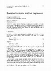12 (1.5, 0.9) (2.1, 0.7) (6.1, 0.2) (6.1, 0.2) (2.1, 0.7) (1.5, 0.9) 1 2 3 a a (2.0, 1.1) (5.1, 0.6) c a a (8.0,1.5) 1 d c 2 c (5.1, 0.6) (2.0, 1.1) b1 b 1 d (8.0,1.5) b2 (0.0, 1.2) (21.0, 0.4) (21.0, 0.4) (0.0, 1.2) Figure 3: Converting a DAG with multiple values per vertex into one with a single value per vertex 6 Multiple Values per Vertex Several authors have considered the extension where there are multiple values at each vertex, i.e., at vertex vi there is a set of weighted values {(yi,j , wi,j ) : 1 ≤ j ≤ ni } for some ni ≥ 1, and the Lp isotonic regression problem, 1 ≤ p < ∞, is to find the isotonic function z that minimizes   ni n X X i=1 j=1 1/p wi,j |yi,j − zi |p  (6) among all isotonic functions. For L2 this simplifies to single-valued isotonic regression where at each vertex the value is the weighted mean Pn of the values and the weight is the sum of the weights, but this is no longer true when p 6= 2. Let N = i=1 ni . Robertson and Wright [19] studied the statistical properties of L1 isotonic regression with multiple values and two independent variables, but no algorithm for finding it was given. Chakravarti [5] gave a Θ(N n) time algorithm for L1 isotonic regression for a tree, and for a linear order Pardalos, Xue and Yong [16] gave one taking Θ(N log2 N ) time, and asked if Θ(N log N ) was possible. A simple approach to this problem is to transform it into one where there is a single value per vertex. Given a DAG G with multiple values per vertex, create a new DAG G′ with one value per vertex as follows: if vertex vi ∈ G has k weighted values (yi,j , wi,j ), 1 ≤ j ≤ k, then in G′ represent vi with vertices vi,j , 1 ≤ j ≤ k; represent edge (vi , vℓ ) in G with edge (vi,k , vℓ,1 ) in G′ ; and add edges (vi,j , vi,j+1 ) to G′ for ′ , w′ ), where y ′ is the j th data value at v in decreasing 1 ≤ j < k. Vertex vi,j has the weighted value (yi,j i i,j i,j ′ is its corresponding weight. See Figure 3. G′ has N vertices and m + N − n edges. An order and wi,j optimal isotonic regression on G′ will have the same value for vi,1 . . . vi,k , and this is the value for vi ∈ G in an optimal solution to (6). The initial sorting at the vertices takes Θ(N log N ) time. An advantage of this approach is that one can invoke whatever algorithm is desired on the resulting DAG. When the initial DAG was a tree the new DAG is as well, and thus the L1 regression can be determined in Θ(N log N ) time. This answers the question of Pardalos et al. and improves upon Chakravarti’s result. For L1 partitioning algorithms another approach is to merely use all N values for the partitioning, resulting in running times that are the same as in Theorem 5.4 where log K is replaced with log N and an N log N term is added, representing the initial sorting of the values and the evaluation of regression error throughout the algorithm. For large N , to reduce the time yet further this approach will be refined. 13 Theorem 6.1 Given a DAG G with multiple weighted values per vertex, with N total values, an L1 isotonic regression can be found in the same running time as in Theorem 5.4, where log K is replaced by log N and an (N + n log N ) log log N term is added. Further, if G is fixed and only N varies then the regression can be found in Θ(N ) time. Proof: It will be shown that O(log N ) stages are needed and that the total time to initialize data structures, find the values used for the binary regressions, and evaluate the regression error, is O((N +n log N ) log log N ). This, plus the time to solve the binary regressions on the DAG, yields the results claimed. For V [a, b], a and b now refer to regression values a and b, rather than their ranks as in Section 2, since their global rank will not be known. The values in (a, b) at the vertices in V [a, b] will be called active values. Rather than finding a median z of all values in (a, b), it suffices to choose an approximate median among the active values. This can be achieved by determining at each vertex in V [a, b] the unweighted median of its active values and weighting this by the number of active values it has. Let z be the weighted median of these medians, breaking ties by choosing the smaller value, and let z ′ be the next largest value at vertices in V [a, b] (if z is b then set z ′ to be b and z the next smallest value). No more than 3/4 of the active values in V [a, b] can be in (a, z) and no more than 3/4 are in (z ′ , b). Hence, no matter how the vertices are partitioned into V [a, z] and V [z ′ , b], in each of them the number of active values is no more than 3/4 of those in V [a, b], and thus there are at most Θ(log N ) iterations until there are no active values. A final partitioning step determines which vertices should have regression value a and which should be b. Initially the values at vertex vi are partially sorted into lg N “bags” of size ni / lg N , where the values in each bag are smaller than the values in the next. For each bag the smallest value, number of values, and sum of weights in the bag are determined. The bags are organized into a binary tree using their lowest value as the key. At each node of the tree is kept the sum of the weights and the number of values in the bags below. This can all be done in Θ(ni log log N ) time at vi , and Θ(N log log N ) time overall. Finding the median of the vertex’s active values, the next largest value above z, and the relative error of using z vs. z ′ , can each be determined by a traversal through the tree and a linear time operation on at most two bags (e.g., to find the relative error of using z vs. z ′ one needs to determine it for values inside the bag where z would go, and then use the tree to determine it for values outside the bag). Thus the time at vi at each stage is Θ(ni / log N + log log N ), and Θ(N/ log N + n log log N ) over all vertices. Since the number of stages is Θ(log N ), this proves the statement at the beginning of the proof. To prove the claim concerning a fixed DAG and varying N no bags are used. Each stage involves multiple iterations, n per stage, where for each vertex the unweighted median of its active values is used for one of the iterations. After each stage the number of active values at a node is no more than half of what it was to begin with, and thus stage k takes Θ(n(T (G) + N/2k )) time, where T (G) is the time to solve a binary-valued L1 isotonic regression on G. Thus the total time is Θ(n(T (G) log N + N )), which is Θ(N ) since G and n are fixed.  7 Final Comments Table 2 is an update of Table 1, incorporating the results in this paper. Results for Lp were not included in Table 1 since polynomial time algorithms had only appeared for linear orderings [1, 7, 26]. The semi-exact algorithms, and the exact L2 algorithms in [14, 21], have a worst-case behavior where each partitioning stage results in one piece having only a single vertex. Partitioning using the mean probably works well in practice, but a natural question is whether the worst-case time can be reduced by a factor of Θ̃(n). 14 ordered set linear L1 Θ(n log n) tree [1, 22] Θ(n log n) 2-dim grid 2-dim arbitrary d ≥ 3 dim grid d ≥ 3 dim arbitrary arbitrary + Θ(n log n) + Θ(n log2 n) + 2 Θ(n log n) * Θ(n2 logd n) + Θ(nm + n2 log n) [2] metric Lp , 1 < p < ∞, semi-exact Θ(n + Tp ), p even Θ(n log n + Tp ), p odd Θ(n2 + Tp ), p arb PAV, + Θ(n log n + Tp ), p integer Θ(n2 + Tp ), p arb [15] (p = 2), + Θ(n2 + Tp ) [21] (p = 2), + Θ(n2 log n + Tp ) + 3 Θ(n log n + Tp ) * Θ(n3 logd n + Tp ) + 2 Θ(n m + n3 log n + Tp ) + Lp , 1 < p < ∞, δ approx Θ(n log K) L∞ Θ(n log n) [1] Θ(n log K) * Θ(n log n) + Θ(n log K) + Θ(n log n log K) + 2 Θ(n log n log K) * Θ(n2 logd n log K) +
2 Θ (nm + n log n) log K + * Θ(n log n) * Θ(n log2 n) [24] Θ(n log n) * Θ(n logd n) [24] Θ(m log n) [24] +: shown here *: implied by the result for arbitrary ordered sets K: (maxni=1 yi − minni=1 yi ) /δ Tp : total data-dependent time to determine Lp means Table 2: Times of fastest known isotonic regression algorithms “Semi-exact” is exact for p = 2, 3, 4, 5, and T2 = T3 = T4 = T5 = 0. Partitioning can also improve the time for L1 isotonic regression for unweighted data on an arbitrary DAG G = (V, E). Partitioning on values a < b is equivalent to finding a minimum vertex cover on the directed bipartite graph H = (V, E ′ ) with vertex partition V1 , V2 , where V1 is those vertices with data ≤ a and V2 is the vertices with data ≥ b. There is an edge (v1 , v2 ) ∈ E ′ , with v1 ∈ V1 and v2 ∈ V2 , iff v2 ≺ v1 in G, i.e., iff they violate the isotonic constraint. Vertices in the minimum cover correspond to those where the value of the {a, b}-valued regression is the further of a or b, instead of the closer. A simple analysis using the fact that the cover is minimal shows that no new violating pairs are introduced. For unweighted √ bipartite graphs the maximum matching algorithm of Hopcroft and Karp takes Θ(E V ) time, from which a minimum vertex cover can be constructed in linear time. H can be constructed in linear time from the transitive closure of G, and since the transitive closure can be found in O(n2.376 ) time (albeit with infeasible constants), the total time over all Θ(log n) partitioning stages is Θ(n2.5 log n). For multidimensional DAGs this can be reduced to Θ̃(n1.5 ) [25]. However, this approach does not help for Lp regression since the binary L1 regression problems generated are weighted even when the data is unweighted. The L1 median, and hence L1 isotonic regression, is not always unique, and a natural question is whether 15 there is a “best” one. A similar situation occurs for L∞ isotonic regression. Algorithms have been developed for strict L∞ isotonic regression [23, 25], which is the limit, as p → ∞, of Lp isotonic regression. This is also known as “best best” L∞ regression [13]. Analogously one can define strict L1 isotonic regression to be the limit, as p → 1+ , of Lp isotonic regression. It can be shown to be well defined, and it is straightforward to derive the appropriate median for a level set [11]. However, like Lp means, this median cannot always be computed exactly. Apparently no algorithms have yet been developed for strict L1 isotonic regression, though PAV is still applicable for linear orders and trees. One can view Proposition 3.2, concerning complete bipartite graphs, and Section 6, concerning multiple values per vertex, as being related. The complete bipartite graph partitions the vertices into sets P1 and P2 . Viewing P1 and P2 as two nodes in a DAG with an edge from P1 to P2 , then the isotonic requirement in Proposition 3.2 is that no element in P1 has a regression value greater than the regression value of any element of P2 , but there are no constraints among elements of P1 nor among elements of P2 . In contrast, the model in Section 6 corresponds to requiring that every element in P1 has the same regression value, and similarly for P2 . The interpretation of multiple values per vertex as partitioning elements, with no constraints among elements in the same partition, can be extended to arbitrary DAGs, resulting in each node of the DAG having an interval of regression values, rather than a single one. A technique similar to that in Section 6 can be used to convert this problem into a standard isotonic regression with one value per vertex, but the special structure can likely be exploited to produce faster algorithms. Finally, the classification problem called isotonic separation [6] or isotonic minimal reassignment [8] is an isotonic regression problem. In the simplest case, suppose there are two types of objects, red and blue, and at each vertex there is an observation of a red or blue object. There is a penalty for misclassifying a red object as blue, and a perhaps different penalty for the opposite error. The goal is to minimize the sum of the misclassification penalties given that red < blue and the classification must be isotonic. This is a straightforward binary-valued L1 isotonic regression problem. In the general case with k ordered categories there is a penalty for misclassifying an object of type i as being of type j. Unfortunately, penalties as simple as 0-1 correct/incorrect do not satisfy the partitioning property in Lemma 2.1. However, for trees, the dynamic programming approach used in Section 3 can be modified to find an optimal isotonic separation in a single pass taking Θ(kn) time. The time required for arbitrary DAGs is unknown. Acknowledgements The author thanks the referees for their helpful suggestions. References [1] Ahuja, RK and Orlin, JB (2001), “A fast scaling algorithm for minimizing separable convex functions subject to chain constraints”, Operations Research 49, pp. 784–789. [2] Angelov, S, Harb, B, Kannan, S, and Wang, L-S (2006), “Weighted isotonic regression under the L1 norm”, Symposium on Discrete Algorithms (SODA), pp. 783–791. [3] Barlow, RE, Bartholomew, DJ, Bremner, JM, and Brunk, HD (1972), Statistical Inference Under Order Restrictions, John Wiley. [4] Brunk, HD (1955), “Maximum likelihood estimates of monotone parameters”, Annals of Mathematical Statistics 26, pp. 607–616. 16 [5] Chakravarti, N (1992), “Isotonic median regression for orders represented by rooted trees”, Naval Research Logistics 39, pp. 599–611. [6] Chandrasekaran, R, Rhy, YU, Jacob, VS, and Hong, S (2005), “Isotonic separation”, INFORMS Journal on Computing 17, pp. 462–474. [7] Chepoi, V, Cogneau, D, and Fichet, B (1967), “Polynomial algorithms for isotonic regression”, L1 Statistical Procedures and Related Topics, Lecture Notes-Monograph Series vol. 31, Institute of Mathematical Statistics, pp. 147–160. [8] Dembczynski, K, Greco, S, Kotlowski, W, and Slowinski, R (2007), “Statistical model for rough set approach to multicriteria classification”, PKDD 2007: 11th European Conference on Principles and Practice of Knowledge Discovery in Databases, Springer Lecture Notes in Computer Sciencce 4702, pp. 164–175. [9] Dykstra, RL and Robertson, T (1982), “An algorithm for isotonic regression of two or more independent variables”, Annals of Statistics 10, pp. 708–716. [10] Gebhardt, F (1970), “An algorithm for monotone regression with one or more independent variables”, Biometrika 57, pp. 263–271. [11] Jackson, D (1921), “Note on the median of a set of numbers”, Bulletin of the American Mathematical Society 27, pp. 160–164. [12] Kaufman, Y and Tamir, A (1993), “Locating service centers with precedence constraints”, Discrete Applied Mathematics 47, pp. 251–261. [13] Legg, D., Townsend, D. (1984), “Best monotone approximation in L∞ [0,1]”, Journal of Approximation Theory 42, pp. 30–35. [14] Maxwell, WL and Muckstadt, JA (1985), “Establishing consistent and realistic reorder intervals in production-distribution systems”, Operations Research 33, pp. 1316–1341. [15] Pardalos, PM and Xue, G (1999), “Algorithms for a class of isotonic regression problems”, Algorithmica 23, pp. 211–222. [16] Pardalos, PM, Xue, G-L, and Yong, L (1995), “Efficient computation of an isotonic median regression”, Applied Mathematics Letters 8, pp. 67–70. [17] Punera, K and Ghosh, J (2008), “Enhanced hierarchical classification via isotonic smoothing”, Proceedings of the International Conference on the World Wide Web 2008, pp. 151–160. [18] Qian, S (1996), “An algorithm for tree-ordered isotonic median regression”, Statistics and Probability Letters 27, pp. 195–199. [19] Robertson, T and Wright, FT (1973), “Multiple isotonic median regression”, Annals of Statistics 1, pp. 422–432. [20] Robertson, T, Wright, FT, and Dykstra, RL (1988), Order Restricted Statistical Inference, Wiley. 17 [21] Spouge J, Wan H, and Wilbur WJ (2003), “Least squares isotonic regression in two dimensions”, Journal of Optimization Theory and Applications 117, pp. 585–605. [22] Stout, QF (2008), “Unimodal regression via prefix isotonic regression”, Computational Statistics and Data Analysis 53, pp. 289–297. A preliminary version appeared in “Optimal algorithms for unimodal regression”, Computing and Statistics 32, 2000. [23] Stout, QF (2012), “Strict L∞ isotonic regression”, Journal of Optimization Theory and Applications 152, pp. 121–135. [24] Stout, QF (2012), “Weighted L∞ isotonic regression”, submitted. www.eecs.umich.edu/˜qstout/abs/LinfinityIsoReg.html [25] Stout, QF (2012), “Isotonic regression for multiple independent variables”, submitted. www.eecs.umich.edu/˜qstout/abs/MultidimIsoReg.html [26] Strömberg, U (1991), “An algorithm for isotonic regression with arbitrary convex distance function”, Computational Statistics and Data Analysis 11, pp. 205-219. [27] Thompson, WA Jr. (1962), “The problem of negative estimates of variance components”, Annals of Mathematical Statistics 33, pp. 273–289. A Computing the Lp Mean The computation of the Lp -mean of a level set for general p is more complicated than for p = 1, 2, or ∞. We are interested in identifying those aspects which might be more than linear in the time of the remainder of the algorithm. We assume that the data values have been presorted. Simple calculus [11] shows that the Lp mean of the data (y, w) is the unique C such that X X wj (C − yj )p−1 (7) wi (yi − C)p−1 = yj <C yi >C which does not, in general, have an analytic solution. An important aspect is to determine the data values that bracket the Lp mean, i.e., to determine which are in the RHS and which are on the LHS of (7). Given the bracketing values, the time to find the mean to desired accuracy may depend upon the data and we make no assumptions concerning it. Given p, n, and data (y, w), the total time to find all Lp means used in the algorithm is decomposed into a part independent of the data and the remaining portion, denoted Tp (n, y, w), that is data dependent. For general p the data independent portion requires evaluating (7) for each set at least once per partitioning stage, and thus Θ(n) time per stage. Since there can be Θ(n) stages in each of the algorithms in Section 5, the data independent time for finding means is Θ(n2 ) once the bracketing values are known. By first partitioning on data values, all of the partitioning algorithms can determine the bracketing values in time no more than the remaining time Pof the algorithm. If p is an even integer, (7) reduces to finding the unique solution of i=1,n wi (yi − C)p−1 = 0, i.e., no bracketing values nor presorting are required. This is a sum of (p−1)st degree polynomials, and hence can be determined by summing up, over the data values, the coefficients of each term and then evaluating the result. For p an odd integer once again the terms are polynomials so, given the bracketing values, one can use sums of coefficients to evaluate the summations in (7). Since roots of polynomials of degree ≤ 4 can be found exactly in constant time, T2 = T3 = T4 = T5 = 0. 18 For PAV sets are merged rather than partitioned. This does not change the data independent time for general p, but for p an even integer each set is reduced to p + 1 coefficients and merging sets merely requires adding coefficients. Hence the data independent time is Θ(n). For p odd the situation is a bit more complex since the bracketing values are needed. One can construct a balanced search tree where data values are keys and at each node, for each term there is the sum of the coefficients beneath it. The only change from being on the LHS vs. the RHS of (7) is whether the term has a plus or minus sign, and hence, given this tree, one can descend through the tree and determine the bracketing data values in logarithmic time. Merging sets corresponds to merging their trees, including maintaining the information about sums of coefficients in subtrees. With careful merging this can be accomplished in Θ(n log n) total time. 19