IEEE TRANSACTIONS ON ELECTROMAGNETIC COMPATIBILITY, VOL. 37, NO. 2, MAY 1995 zyxwvutsr 221 zyxwvut zyxw zyxwvutsrqpon zyxwvut zyxwvu a A zyxwvutsrq zyxwvutsrqp zyxw Electromagnetic Topology: Investigations of Nonuniform Transmission Line Networks Phillippe Besnier and Pierre Degauque, Member, ZEEE Abstract- The electromagnetic topology approach is often used to calculate the current or voltage that can appear on a transmission line network illuminated by a disturbing wave. However the lines are supposed to be parallel to a ground plane and, furthermore, the model has often been applied on canonical cases. In this paper, a generalization of this formalism to treat nonuniform transmission l i e s is presented. Moreover, by treating a wiring installed inside a Transall airplane mockup, a comparison between theoretical and experimental results shows the validity and the interest of this approach. 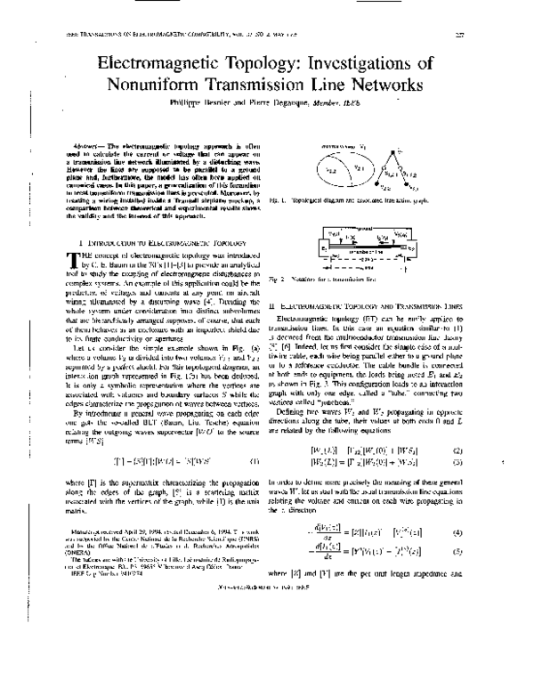external volume V1 %2,1 v2,2 s1.2.2 “2,l Fig. 1. Topological diagram and associated interaction graph. I , ground I. INTRODUCTION TO ELECTROMAGNETIC TOPOLOGY T HE concept of electromagnetic topology was introduced by C. E. Baum in the 70’s [ 11-[3] to provide an analytical 4 - - - --z-axis - - - - L I tool to study the coupling of electromagnetic disturbances to Fig. 2. Notations for a transmission line. complex systems. An example of this application could be the prediction of voltages and currents at any point on aircraft wiring illuminated by a disturbing wave [4]. Dividing the 11. ELECTROMAGNETIC TOPOLOGY AND mANSMISSI0N LINES whole system under consideration into distinct subvolumes Electromagnetic topology (ET) can be easily applied to that are hierarchically arranged supposes, of course, that each transmission lines. In this case an equation similar’to (1) of them behaves as an enclosure with an imperfect shield due is deduced from the multiconductor transmission line theory to its finite conductivity or apertures. Let us consider the simple example shown in Fig. l(a) [5]-[6]. Indeed, let us first consider the simple c k e of a mulwhere a volume V, is divided into two volumes V2,1 and V Z , ~ tiwire cable, each wire being parallel either to a ground plane separated by a perfect shield. For this topological diagram, an or to a reference conductor. The cable bundle is connected interaction graph represented in Fig. l(b) has been deduced. at both ends to equipment, the loads being noted El and E2 It is only a symbolic representation where the vertices are as shown in Fig. 2. This configuration leads to an interaction associated with volumes and boundary surfaces S while the graph with only one edge, called a “tube,” connecting two edges characterize the propagation of waves between vertices. vertices called “junctions.” Defining two waves WI and W, propagating in opposite By introducing a general wave propagating on each edge one gets the so-called BLT (Baum, Liu, Tesche) equation directions along the tube, their values at both ends 0 and L relating the outgoing waves supervector [WO] to the source are related by the following equations terms [WS] zyxwvutsrq [r] where is the supermatrix characterizing the propagation along the edges of the graph, [SI is a scattering matrix associated with the vertices of the graph, while [l] is the unit matrix. Manuscript received April 29, 1994; revised December 6, 1994. This work was supported by the Centre National de la Recherche Scientifiaue (CNRS) and bi‘the Office National de d’Etudes et de Recherches Akrospatiales (ONERA). The authors are with the University of Lille. Laboratoire de RadiouroDagation et Electronique, Bat. P3, 59655 Villeneuve d’Ascq Ckdex, France. IEEE Log Number 9410274. In order to define more precisely the meaning of these general waves W ,let us start with the usual transmission line equations relating the voltage and current on each wire propagating in the z direction -~ d[vl(z)l = [Z][I1(z)]- [V,’“’(Z)] dz (4) .- where [Z] and [Y] are the per unit length impedance and 0018-9375/95$04.00 0 1995 IEEE zyxwvu zyxw IEEE TRANSACTIONS ON ELECTROMAGNETIC COMPATIBILITY, VOL. 31, NO. 2, MAY 1995 228 admittance matrices, respectively. [I,("] and [V,'"'] are source vectors, either of current or of voltage, distributed along the conductors. New variables for voltages and voltage sources are introduced where [Zc] is the characteristic impedance matrix. If a propagation matrix [y] is defined by of the ( 2 )and (Y) matrices remain constant and independant on z . However nonuniform bundles have to be considered in order to be able to treat more realistic configurations frequently found in industrial electronic systems. We have already supposed implicitely that a quasi-TEM mode is supported by the cable network to establish the transmission line equations, providing the vicinity of grounding conductors. As far as we are concerned by nonuniform lines, it seems to be very hazardous to use a quasi-TEM approximation again. We can assume that these structures are often slightly nonuniform ones. Even if it isn't true,'and for very good conductors, the TEM mode approximation must appear, not in a general sense as small field amplitudes in the longitudinal direction of the cable bundle, but in the vicinity of each conductor direction. Then, there is TEM approximation with respect to each individual conductor. If the wires inside a tube are non-parallel ones, the differential equations of the transmission line theory are much more difficult to solve. From the topological approach, we have seen that the solution of voltage and current distribution along a single uniform tube can be expressed in terms either of a forward or of a backward wave. Coming back to the expression of the total voltage, if we consider the propagation along the positive z axis and, to simplify the notation by putting ( V ) = (VI(.)), one gets zyxwvutsrqp zyxwvutsrqponml zyxwvutk where p.v. means "the principal value of them," the system (4) and ( 5 ) can be written as d[vl(z)l+ dz + [y][V1(z)]+= [V,'"'(.)]+ d[V1(z)l- - [y][&(z)]- = [v;"'(z)] dz (11) _. (12) The integration of (1 1) over the length L of the bundle leads to -(Z(z))(Y(z))(V(z)) = 0 (14) where the matrices ( 2 )and (Y) are z-dependant. The differential equation verified by I ( z ) is the dual one and is obtained by interchanging ( 2 ) and (Y). Equation (14) can be solved for very simple nonuniform structures or for some kinds of configuration that can be treated in terms of circulant matrices [?I. One shows, in this case, that if matrices of (14) are circulant ones, then they are diagonalized by the same so-called Fourier matrix. Then (14) is scalarized and can be solved, for instance, by a perturbation method to find resonance frequencies of a slightly diverging pair of wires [12]. However, it seems difficult to treat all kinds of nonuniform structures by an analytical means, even if some attempts have been undertaken to reach this goal [8]-[lo]. In order to develop a very general tool, we suggest to extend the resolution of the BLT equation to nonuniform multiconductor transmission lines (NMTL) by introducing a discretization method. This approach simply consists in approximating a NMTL by a series of successive uniform multiconductor transmission lines (UMTL). After evaluating the per unit length impedance and admittance matrices for each section of the discretized bundle, scattering parameters are calculated at the discontinuities, thus at the junctions between the various sections, the whole network being then solved through the BLT equation. These discontinuities introduced by the discretization are purely fictive and are not to be considered as radiation sources. However, they create artificial reflecting planes that are minimized by increasing the number of discretization elements. In the following, this method is illustrated first zyxwvutsrqpon zyxwvutsrq The comparison of the mathematical form of (2) and (13) allows to define all the matrices of (2). Likewise, the various terms of (3) can also be deduced from (11) but by introducting an axis z, having its origin at z = L and with an opposite direction to the one of the z axis (Fig. 2). The voltages and currents associated with this z, axis are noted V2(2,) and Iz(z,). It is obvious that Vz(z,) = V l ( L - z,) and that I2(z,) = - I l ( L - 2 , ) . To sum up, the various terms of (2) and (3) are given by 111. EXTENSION TO NONUNIFORM nANSMISSION LINESDISCRETIZATION METHOD The tube schematically represented in Fig. 2 has implicitely been chosen an uniform one. It means that its geometry is the same all along the bundle axis and, as a consequence, the terms BESNIER AND DEGAUQUE ELECTROMAGNETIC TOPOLOGY Fig. 3. 229 zyxwvutsrqponm Two nonparallel wires over a ground plane. zyx Fig. 4. Discretization of the two nonparallel wires. in the simple case of two non-parallel wires and then in a more complicated structure corresponding to an experimental approach carried out on a Moth Transall airplane mockup. Then the mutual capacitance remains the same whatever the orientation of wire 2. In summary, ( L ) an! (G) matrices are written as zyxwvuts zyxwvutsrqponm zyxwvutsrq zyxwvutsrq zyxwvutsrq zyxwvuts zyxwvutsr Iv. DISCRETIZATION METHODAPPLIEDTO THE CASE OF TWO NONPARALLEL WIRES This configuration has been widely discussed by J. Nitsch et al. [12] since an analytical solution can be obtained. This will enable us to compare this solution to the results obtained with the discretization method and, thus, to study convergence problems. As shown in Fig. 3, let us consider two wires situated at the same height above a perfectly conducting ground plane but diverging with an angle 28. It is assumed that these bare wires are situated inside an homogeneous medium characterized by its permittivity E and its permeability p. In a first step the inductance ( L ) and capacitance ( G ) matrices for two nonparallel elements are determined. We recall that for two parallel wires having a diameter d, situated at a distance D from each other, at a height h above a ground plane, the per unit length inductance and capacitance matrices, noted in this case ( L p )and (C,) are given by (L,) = P(9) (CP)= Ek7-l (15) where the various terms of (9)are easily determined if D >> d (5) 911 = Q22 = -Log. Q12 = g21 = -47r LO.,(l+ 2T $). In the case of diverging wires, the position of any point along these wires is referred to by its abscissa 21 and z2, the origin being chosen at one end of the wire. Furthermore, due to the symmetry of the geometrical configuration, one can also introduce an absolute value for the abscissa defined by z = z1 = 22. The distance D(z) between the wires is thus given by D(z) = Do + 22 sin 8. (16) DO being their distance at the origin. The angle 28 between the wires modifies the mutual inductance. Indeed, if a current Il flows over an element dzl of wire 1, the magnetic flux at the same abscissa on wire 2 is reduced by a factor cos 28. On the other hand, the mutual capacitance has not changed in nature and only depends on the distance between the wires. Indeed, the electric field created by charges on an element dzl on wire 1, due to the presence of a parallel ground plane, is uniform around the element dz2 on wire 2. Each wire of length 1 is divided into N elements as shown in Fig. 4. The coupling between wires 1 and 2 for the ith element, is calculated from formulas (17) for ( L ) and (G) approximating D ( z ) by a constant Di given by 2i - 1 D, = Do + -( D L - D o ) 2N 15i 5.N (18) where DOand D L are the distance between the wires at z = 0 and z = 1. The order of the discretization, i.e., the number of elements, is obtained by using a convergence criterion and thus by comparing the results for N and 2N elements..The structure is thus divided into N successive tubes, the two wires inside each tube being connected by a short circuit. The topological scattering parameters at each junction can either be determined theoretically or experimentally deduced from the scattering parameters measured on 504 loads. In the case of the junction between two tubes being only made with short circuits, mathematical difficulties appear and we have already shown that they can be avoided by expressing the S parameters in terms of characteristic impedance matrices of each tube [ 111. In order to check the validity of this approach, an example already treated by Nitsch et aZ, [12] has been choosen. The wires, 3 m long and situated at a height of 3 cm above the ground plane, are slightly diverging since their distance varies from 0.5 cm at one end to 1.5 cm at the other end. Applying a perturbation method, Nitsch et al. [12] have shown that if the wires are opened at both ends, the natural resonance frequency fo associated with parallel wires is split in this case into two resonance frequencies f l and f 2 . In this example f o = 50 MHz, the perturbation method applied to the diverging wires leading to f l = 49.53 MHz and f 2 = 50.18 MHz. Numerically, by dividing the structure into 32 tubes, we get f l = 49.46 MHz and f 2 = 50.19 Hz. v. EXPERIMENT ON A 1/1()THTRANSALL AIRPLANE MOCKUP In order to validate the topological approach for noncanonical cases, we have considered a more realistic configuration by putting a cable network inside a l/lOth Transall mockup shown zyxwvu zyxw zyxwv zyxwv IEEE TRANSACTIONS ON ELECTROMAGNETIC COMPATIBILITY, VOL. 31, NO. 2, MAY 1995 230 distance between wires :2,5 cm ground (fuselage) Fig. 6. Height of the bifilar line over a fictive flat ground plane. transfer function (dB) zyxwvutsrqpo n zyxw Photo 1. The l/lOth TRANSALL mockup (Source: ONERA) 1 dl 2 4 6810 20 4 0 6 0 ~ 1 1 M 2400 ~ frequency (MHz) Fig. 7. Bifilar line in the back fuselage modeled by a single tube. A. BiJilar Line Inside the Back Fuselage zyxw I n6 wing fuse'age / Fig. 5. TRANSALL network (detailed connexions of IB are given in Fig. 14). in Photo 1, each insulated copper wire having a diameter of 1.2 mm. It is difficult to precisely define the position of all the cables running along the structure, but globally the airplane can be divided into five parts: the two wings, the back and front fuselage, and a central part where all the cables are interconnected. Various types of bundles have been installed, such as a bundle of six wires slighty diverging from one end to the other, a crossing of wires in the middle of the wings. A schematic representation of the network is given in Fig. 5. We have proceeded step by step, considering first each part of the airplane separately before simulating the global response of the network. A two-wire line has been tightened in the back fuselage. Due to the shape of this fuselage, the relative height of the line with respect to the metal changes smoothly but there are also abrupt changes due to the presence of spars. By considering a fictive flat ground plane, the geometrical configuration is shown in Fig. 6, the wire spacing being equal to 2.5 cm, Both the theoretical and experimental transfer functions characterizing the response of these two conductors have been determined. This transfer function is defined as the ratio between the voltage at one end of a wire to the voltage delivered by the source connected on the second wire, the two other ends being loaded into 50 0. In order to point out the influence of a fine discretization, various lengths of tubes have been considered. If the bifilar line is first modeled with the help of a single tube situated at a constant and thus average height above the ground plane, curves in Fig. 7 show that the agreement between the theoretical results and the experimental ones, also represented in this figure, is rather good in the low frequency domain, below 60 MHz in this case. It must be noted that the capacitance and inductance matrices have been analytically calculated from (15) and not measured. The discrepancy in the high frequency range can of course be explained by the various abrupt discontinuities occuring along the line due to the spars. To point out this effect, four tubes have been introduced, associated with each constant height of the bundle, while a fifth tube corresponds to the average height of the first part of the geometrical configuration. As it appears in Fig. 8, the improvement is quite noticeable in the 200-500 MHz range. Lastly, by solving the BLT equation with eight tubes, allowing a discretization of both the inclined part and the abrupt discontinuities, the agreement between the theoretical and experimental results becomes quite good in all the frequency range under consideration (Fig. 9). zyxwvutsrqpo zyxwvutsrqpo 23 I BESNIER AND DEGAUQUE: ELECTROMAGNETIC TOPOLOGY zyxwvutsrqponmlkjihg zyxwvutsrqponmlkjih zyxwvutsrqponmlkj transfer function (dB) 1 2 3 -4 5 6 7 1 2 4 6 6 10 20 406080100 200 400 50 Ohms frequency (MHz) Fig. 8. Comparison between simulation of the bifilar line in the back fuselage with partial average height and experimental results. wire I transfer function (dB) 1 I 50 Ohms Oh A I hl=2,5 cm h2=2,0 cm dl=d2=0,18 cm ' Fig. 10. Crossing wires over a ground plane. Angle 30" .I 1 2 4 6 8 10 20 406080100 200 400 frequency (MHz) Fig. 9. Comparison between simulation of the bifilar line in the back fuselage by a full discretization method and experimental results. zyxwvutsrq 1 2 4 4060801W 2W 20 6 8 10 4w frequency (MHz) B. Crossing Wires zyxwvutsrq zyxwvut zyxwvuts zyxwvutsrq Crossing wires are nonparallel wires, but noncoupled on their whole length. Outside the coupling zones, the bundles are thus treated by introducing two or more different tubes, while inside the coupling zone all the wires are included in the same tube. The maximum length of this tube I d , starting from the crossing point defined by z1 = z2 = 0 (Fig. 10) is such that the ratio R, of the mutual inductances calculated at z1 = z2 = ZI = Z d p and at z1 = 2 2 = 0 is smaller than a given value Rt, arbitrarily chosen. In other words, it means that beyond 21, the mutual coupling between the tubes are neglected. The mutual inductance has been chosen as a criterion but, of course, the mutual capacitance can also be considered, especially in the case where the wires are orthogonal. For large angles between the wires one could as well evaluate a local inductive and capacitive coupling [14]. Introdution of lumped elements for crossing wires depends on the length of the coupling zone and on the frequency range under investigation. A numerical parametric study has first shown that Rt must be equal to -40 dB to reach a good convergence, the results being not changed more than 1 dB if a smaller value of Rt is chosen. For the geometrical configuration represented in Fig. 10, curves in Fig. 11 represent the variation of the transfer versus ~ ~ frequency, for two angles of the function V L ~ / V wires: 30" and 70". The agreement between the theoretical and experimental results is quite correct, each wire being divided into 32 tubes to reach the required accuracy. (a) Angle 70' 1 2 3 frequency (MHz) (b) Fig. 11. Results of experiments performed on crossing wires with angles of 30' and 70'. 3.022.38 3.87 3.03 3.34 4.29 2.7 3.45 1.74 2.19 2.06 2.61 1.42 1.77 1.1 0.46 1.35 0.51 0.78 0.93 1.01 1.01 0.54 0.54 distance 1.2 distance 2.3 Fig. 12. Nonparallel wires in the left wing. zyxwvutsrq C. Nonparallel Wires in the Left Wing Converging and then diverging wires have been installed in the left wing as shown in Fig. 12. This three-wire structure has been modeled with 12 tubes. All the ends are loaded on 50 0, the excitation point being g1 while g3 is the point of calculation. The theoretical and experimental variations of the transfer function between these two points are given in Fig. 13 and the agreement between these results is rather good in a wide frequency range. zyxw zyxwvutsrqponmlkj IEEE TRANSACTIONS ON ELECTROMAGNETIC COMPATIBILITY, VOL. 37, NO. 2, MAY 1995 232 transfer function (dB) transfer function (dB) .lEZ3=ZE3 1 zyxwvutsrqponmlkjihgfedc zyxwvutsrqponmlkjih 2 4 6 8 10 20 4060g01W2W 40 1 4M) frequency (MHz) I 2 4 6810 20 4oBoBolW200 4M) frequency (MHZ) Fig. 13. Nonparallel wires in the left wing: results. Fig 15 Global results transfer function between points H1, up in the rmddle of the wings and N1 at the TRANSALL’s nose, See Fig 5 To forward fuselage TO gl - To left wing To nght wing - TO K2 ; ;1 shielded box ;1 zyxwvutsrqpon zyxwvuts zyxwvu frequency (MHr) To backward fuselage Fig. 14. Wiring of the interconnection box ( d 3 is connected to 93 without passing through the IB). D.Global Test Each part of the network has been then tested separately in order to check the validity of the method and to have an order of magnitude of the difference between theoretical and experimental values of the transfer function determined at various points. In a last step, all the wires are interconnected in a shielded box, the connections being short circuits between various wires at it appears in Fig. 14. In the topological model, a first possibility is to consider this box as a black box. It means that the topological scattering parameters of this 13-port junctions are deduced from the S parameters measured on 50 R [3]-[13]. Another possibility is to calculate the topological S matrix, knowing the interconnection scheme and by neglecting the propagation effect inside the box. Indeed, the maximum dimension of the box is 10 cm and the circuit can be replaced by lumped elements. Both approaches have been tested and give nearly the same results. The total network has been divided into 70 tubes, with 410 components for the [Wd]vector. Transfer functions have been calculated between various excitation and measurement points on the wires. As an example, curves in Fig. 15 represent the variation of the transfer function between the end of the wire situated in the middle of the fuselage, point hl in Fig. 5 and the end of another wire running in the front fuselage and located in the airplane nose (point nl). In the low frequency range, the agreement between theory and experiment is very good and then the first two resonance frequencies are well predicted by the model. For the highest order resonances, the discrepancy can be explained by an inaccurate evaluation of the capacitance and inducance matrices, each term of these matrices, associated with each tube, being calculated by means of simple analytical formulas assuming that the wires are put over a ground plane, or sometimes measured. Fig. 16. Global results: transfet function between points Ai3 and N 4 at the TRANSALL’s nose. See Fig. 5 . The last example in Fig. 16 corresponds to the transfer function between the points n3 and n4 (Fig. 5) and shows that even for a noncanonical geometrical structure, the total response is correctly predicted at least up to the second or third resonance frequencies. zyxwvutsrq VI. CONCLUSION A discretization method has been used to treat nonuniform transmission lines, since such a configuration can then be handled very easily through a topological approach. This method was first tested on canonical examples such as diverging or crossing wires. Lastly a global test has been performed on a complicated network installed inside a TRANSALL mockup and the good agreement between theoretical and experimental results prove the feasibility of this method. Recently, electromagnetic topology has been successfully applied to the Philips Laboratory test-bed aircraft (EMPTAC) [15]. ACKNOWLEDGMENT The authors especially thank Mr J. C. Alliot, head of the EMC department in ONERA, he authorized us the use of the TRANSALL mockup and the equipment associated with the experiments. These experiments were carried out with the precious help of Mr. P. le Helloco, ONERA. REFERENCES [ I ] C. E. Baum, “How to think about EMP interaction,” Proc. Spring Fulmen Meeting (Fulmen 2), pp. 12-23, Apr. 1974. 121 __ , “The theory of electromagnetic interference control,” Interacfion Notes, Note 478, Dec. 1989. [3] F. M. Tesche, “Topological concepts for internal EMP interaction,” IEEE Trans. Electmmagn. Compat., vol. 20, no. 1, pp 60-64, Feb. 1978. [4] J. P. Parmantier, G. Labaune, J. C. Alliot and P. Degauque “Electromagnetic coupling on complex systems: Topological approach,” Inferaction Nore 488, May 1990. zyxwvutsrqpo zyxwvutsrqpo zyxwvutsrqponm zyxwvutsrqpo zyx zyxwvutsrq zyxwvutsrqponmlk BESNIER AND DEGAUQUE: ELECTROMAGNETIC TOPOLOGY [5] F. M. Tesche and T. K. Liu, “Application of multiconductor transmission line network analysis to intemal interaction problems,” Electmmgneticy, vol. 6, no 1, 1986. ’ [6] J. P. Parmantier, “Approche topologique pour I’etude des couplages electromagntttiques,” These de Doctorat, Universitb de Lille, France, Dec. 1991. [7] J. Nitsch, C. E. Baum, and R. Sturm, “Analytical treatment of circulant nonuniform multiconductor transmission lines,” fEEE Trans. Elecrromugn. Ciimpat., vol. 34, no. 1, pp. 28-38, 1992. [SI M. Leiniger and H Schmeer, “A new method to evaluate the propagation of electromagnetic waves on inhomogeneous transmission lines,” in Proc. 8th Int. Zurich Symp. Electrumagn. Compar., Mar. 1989, pp. 29 1-29b. [9] K. Kobayashi, Y.Nessoto, and R. Sato, “Equivalent representations of nonuniform transmission lines based on the extended kuroda’s idenditv,” IEEE Trans. Microwave Theory Tech., vol. 30, pp. 14CL-146,Feb. 1982. [ 101 M. 3. Ahmed, “Impedance transformation equations for exponential, cosine-squared and parabolic tapered transmission lines,” IEEE Trans. Microwave Theoty Techn., vol. 29, no. 1, pp. 67-68, 1981. [ 1 I ] Ph. Besnier and P. Degauque, “Probltmes lies h la determination des parametre S (scattering) de jonctions en topologie tlectromagnetique,” Annales des TtWcommunications, 1995, to be published. [ 121 J. Nitsch and C. E. Baum, “Splitting of degenerate natural frequencies in coupled two conductor lines by distance variation,” Interaction Notes, Note 477, July 1989. [I31 P. Besnier, “Etude des couplages 6lectromagnCtiques sur des reseaux de lignes de transmission non uniformes h I’aide d’une approche topologique,” These de Doctorat, UniversitC de Lille, France, Janvier, 1993. [ 141 D. V. Giri, S. K. Chang, and F. M. Tesche, “A coupling model for a pair of skewed transmission lines,” IEEE Trans. Electromagn. Compat., vol. 22, pp. 2C-28, Feb. 1980. [15] J. P. Parmantier, V. Gobin, F. Issac, I. Junqua, Y. Daudy. and J. M. Lagarde, “An application of the electromagnetic topology theory to the test bed aircraft EMPTAC,” heraction Note 506, pp. 3 1 4 8 , Nov. 1993. 233 Philippe Besnier was bom in Melesse, France, on June 7, 1967. He received the degree in electronic engineering from the Ecole Universitaire D’Ingknieurs de Lille in 1990, and the Ph.D. degree from the University of Lille in 1993. He joined ONERA for one year in 1993 in the EMC department. He is currently chargC de recherches au CNRS in the Laboratoire de Radio Propagation et Electronique of the university of Lille His research interests are mainly focused on electromagnetic compatiblity and derivation of intemal coupling problems. Pierre Degauque (M’76) was born in Lille, France, on Sept. 19, 1946. He received the M.S. and Ph.D. degrees from the University of Lille in 1966 and 1970, respectively. He also received a degree in electronic engineenng from the Institut Sup6rieur d’Electronique du Nord, Lille, in 1967 Currently, he is a Professor at the university of Lille. Since 1967, he has been working at the Laboratoire de Radio Propagation et Electronique in the field of electromagnetic wave propagation and radiation from various antenna configurations His pnmary interest is in radiation problems associated with antennas situated in absorbing media for geophysical applications. He has contnbuted to studies of radiopropagation in mines via leaky braided coaxial cables, and is actlve in research on electromagnetic compatibility including wave penetration into structures and coupling to transmission lines Dr. Degauque is a member of the IEEE Electromagnetic Compatibility Society, the IEEE Geoscience and Remote Sensing Society, and the IEEE Antennas and Propagation Society, and is responsible for the French Commitee of URSI.