On-line Joint QoS Routing and Channel Assignment in
Multi-Channel Multi-Radio Wireless Mesh Networks✩
Bahador Bakhshia , Siavash Khorsandia,∗, Antonio Caponeb
a Computer
Engineering and Information Technology Department, Amirkabir University of
Technology, Hafez Avenue, Tehran, Iran
b Department of Electronics and Information, Politecnico di Milano, Piazza Leonardo da
Vinci 32, 20133 Milan, Italy
Abstract
We study the problem of on-line joint QoS routing and channel assignment for
performance optimization in multi-channel multi-radio wireless mesh networks,
which is a fundamental issue in supporting quality of service for emerging multimedia applications. To our best knowledge, this is the first time that the
problem is addressed. Our proposed solution is composed of a routing algorithm that finds up to k but not necessarily feasible paths for each demand
and an on-demand channel (re)assignment algorithm that adapts network resources to maintain feasibility of one of the paths. We also study the problem
of obtaining an upper bound on the network performance. First, we consider
an artificial version of the problem, in which all demands arrive at the same
time, and formulate it as a mixed integer linear programming model. To tackle
the complexity of the model, it is relaxed that provides a tight upper bound
while improves solution time up to 3.0e+5 times. Then, we model the original
problem by extending the relaxed model to consider dynamic demands, it leads
to a huge model; thus, we develop another model, which is equivalent to the
first one and is decomposable. It is broken down by a decomposition algorithm
into subproblems, which are solved sequentially. Our extensive simulations show
that the proposed solution has comparable performance to the bound obtained
from the decomposition algorithm; it efficiently exploits available channels, and
needs very few radios per node to achieve high network performance.
Keywords: Joint QoS Routing and Channel Assignment, Optimization
Model, Decomposition, Upper Bound, Multi-Channel Multi-Radio Wireless
Mesh Networks
1. Introduction
QoS of Service (QoS) support, which is entailed by emerging multimedia services, is an essential component in broadband Wireless Mesh Networks (WMN).
✩ This work was done while Bahador Bakhshi was a visiting PhD student at Politecnico
di Milano and was supported through funds provided by Iran Telecommunication Research
Center (ITRC) and the Italian PRIN project SESAME.
∗ Corresponding author
Email addresses: bbakhshi@aut.ac.ir (Bahador Bakhshi), khorsandi@aut.ac.ir
(Siavash Khorsandi), capone@elet.polimi.it (Antonio Capone)
Preprint submitted to Computer Communications
February 19, 2011
It is challenging since multimedia services require intensive resources and the
capacity of WMNs is shrunk by the interferences arise from the shared nature
of the wireless media. Multi-channel multi-radio networking is a promising approach to mitigate the interferences and boost network capacity.
The main problem is to maximize network performance while maintaining
QoS requirements. Contrary to the traditional network throughput maximization problem, in this problem, the network performance is measured in terms of
acceptance rate of QoS sensitive traffic demands. A demand is accepted if the
network can meet its QoS requirements. Due to the fact that bandwidth is the
most important QoS requirement for multimedia applications, which influences
other requirements such as delay jitter as well [1], we focus on this requirement.
Consequently, in the problem studied in this paper, a demand is accepted if
there is a path with sufficient bandwidth that is named feasible path.
Existence of the feasible path depends on available bandwidth of links, which
is specified by channel assignment pattern and flow routes. It depends on channel assignment because each link has to share its physical channel capacity with
other interfering links, which are determined by the channel assignment. Flow
routing affects links available bandwidth as it specifies the load on each link.
Therefore, to maximize the network performance, routing path of flows and
channels of links should be jointly optimized that leads to the joint QoS routing
and channel assignment problem. Although a few solutions have been proposed for both QoS routing and channel assignment problems in multi-channel
multi-radio WMNs, the joint problem has not yet been studied.
The existing algorithms for QoS routing problem [2–12] either do not consider the multi-channel nature of the network or assume that channel assignment
is performed before loading the network, and it is fixed. The solutions obtained
by these algorithms are suboptimal as they are not capable of adapting network resources according to traffic demands. Furthermore, their performance
depends on the channel assignment algorithm.
The proposed channel assignment schemes in the literature are classified
into two broad categories: static and dynamic1 [13, 14]. In the former category,
channels are assigned for a long period of time while in the latter, channels
may be reassigned frequently over time according to needs. Static methods are
oblivious to dynamics of network traffic; consequently, they give suboptimal
network performance. On the other hand, dynamic approaches aim to achieve
better performance by adapting network resources for traffic demands. However,
existing dynamic channel assignment algorithms [15–20] do not consider endto-end QoS requirements of flows and are not coupled with routing.
In this paper, we study the on-line joint QoS routing and channel assignment
problem. In this problem, it is assumed that each demand arrives at a particular
time and requires a specific bandwidth. The demand is accepted if we can find
a path with sufficient bandwidth, otherwise it is rejected. The primary goal
is to maximize acceptance rate of the demands by jointly optimizing routing
and channel assignment. We assume that routing and channel assignment are
parts of the network management tool, so they are centralized algorithms and
run on the call admission control (CAC) server, which has a fairly accurate
1 Fast switching is a special case of the dynamic approaches in which channels are changed
per-packet. The method needs particular MAC protocol and is not considered in this paper.
2
and complete view of the network. It should be noted that in spite of existing
many solutions for the joint routing and channel assignment problem, they are
not applicable to this problem because they do not consider end-to-end QoS
requirements and are off-line schemes.
Our contributions to the on-line joint QoS routing and channel assignment
problem are as follows.
• We formulate the problem and identify the design requirements of the
algorithms for QoS routing and channel assignment subproblems.
• We design the QoS Driven Dynamic Channel Assignment (QDDCA) algorithm as an efficient resource management tool to adapt network resources
according to traffic demands.
• We develop a k-shortest path based on-line QoS routing algorithm. This
algorithm and QDDCA are integrated in the Joint QoS Routing and Channel Assignment (JQRCA) algorithm to provide an efficient solution for the
problem.
• We propose a technique to obtain an upper bound on the network performance. We develop an optimal mixed integer linear programming (MILP)
model for an artificial version of the problem, in which demands are static.
Due to intractability of the model, we relax it to get an upper bound. By
extending the relaxed model to dynamic demand case, we model the original problem. Since it leads to an enormous model; we develop a decomposition algorithm which splits the problem into many small subproblems
and solves them sequentially.
The remaining of this paper is organized as follows. In Section 2, we review
the related work and highlight shortcomings of existing solutions to apply them
on this problem. Assumptions, system models, and problem statement are
presented in Section 3. We explain the main ideas of our solution in Section 4.
The QDDCA algorithm is presented in details in Section 5. Section 6 explains
the JQRCA algorithm. The technique to obtain an upper bound on the network
performance is explicated in Section 7; moreover, in this section, we present the
simulation results to show the efficiency of the technique. Simulation results
to evaluate the performance of JQRCA under various settings of network and
traffic parameters are presented in Section 8. Finally, Section 9 concludes this
paper.
2. Related Work
In this section, we review three categories of related work including QoS
routing algorithms in WMN, dynamic channel assignment schemes, and solutions proposed for the joint routing and channel assignment problem.
There are a number of studies on the problem of finding feasible path in
WMN [2–5] since it is NP-Complete in multi-hop wireless networks [21, 22]. A
genetic algorithm was proposed in [2] and in [3–5], flooding based algorithms
were developed. The key issues in this problem are to estimate link available
bandwidth and control admission of demands, which have been studied in [6–
8]. However, these solutions only focus on finding a feasible path and do not
consider the network performance optimization problem.
3
The problem of optimizing network performance has been studied in [9–11].
In [9], the authors proposed a routing metric to find the cost-effective paths.
The proposed routing metric in [10] considers link available bandwidths and
channel diversity. A hop-count bounded heuristic algorithm was proposed in
[11] that finds the feasible path with the maximum bottleneck capacity. Although these solutions attempt to maximize network performance, they assume
that channel assignment is fixed; thus, their performance depends on the given
channel assignment. The authors in [11] and [12] considered the channel assignment problem besides QoS routing, but they did not solve the joint problem.
In both solutions, there are two phases; in the first phase, a static load-unaware
channel assignment is performed and the second phase is QoS routing.
The previous work on dynamic channel assignment in multi-channel multiradio WMN can be viewed in two categories [13]: the approaches designed to
mitigate external interference [15–17] and the solutions that reassign channels
based on local load measurements [18–20]. In the first category, there is an external source of interference, nodes measure interference periodically, and switch
to the least interfered channel. Although minimizing the external interference
improves network performance, this category does not explicitly consider network traffic, its dynamics, and QoS requirements. In the second category, each
node measures its link loads and if detects an overloaded link, changes the channel of the link. These solutions attempt to improve the one-hop capacity of the
network but cannot guarantee the end-to-end bandwidth requirement of flows,
which is the main constraint in supporting QoS.
Combinations of channel assignment and other problems, including routing,
scheduling, and power control have been the subject of many studies [23–34].
The goal of these joint problems is to maximize network throughput subject
to a fairness constraint. The number of adjustable parameters is the factor
makes the difference between these studies. A group combined routing and
channel assignment [23–27], while some others studied the joint problem of
routing, channel assignment, and scheduling [28–31]. Another group even took
the power and/or rate control into account [33, 34].
We have a closer look at the joint routing and channel assignment algorithms
[23–27]; the second and third groups are beyond the scope of this paper. In [23],
an iterative algorithm was proposed; for a given set of flows, the algorithm iteratively adjusts routing and channel assignment as long as it can improve network
throughput. The authors in [24] developed a simulated annealing based method
to find the optimal channel assignment and routing. The idea of the solution in
[25] is to split a large optimization problem into many small subproblems. The
subproblems are solved independently, and the final feasible solution is obtained
after post processing. The architecture proposed in [26] uses multipath routing
and meanwhile attempts to minimize the interference between multiple paths of
each flow. The joint routing and channel assignment problem was modeled as
a non-linear mixed integer problem in [27]; after linearization, the authors used
the dual decomposition methods to find a near optimal solution.
These solutions are not applicable to the on-line joint QoS routing and channel assignment problem for the following reasons. First, the desired objective,
maximizing per-flow achievable rate, is different from the goal of the joint QoS
routing and channel assignment in which the number of admitted demands
should be maximized. Second, these solutions are off-line; they need information of all flows at the beginning. Third, when traffic pattern changes, e.g., a
4
Notation
V
E
∆
K
TR
IR
ru
p
Ψ
(u, v)
ck(u,v)
I(u,v)
′
I(u,v)
Iˆ
Ψ
w(u,v)
l(u,v)
k
l(u,v)
i
f(u,v)
Φ
Table 1: Notations
Description
Set of nodes and |V | = n.
Set of edges and |E| = m.
Set of demands, ∆ = {δi = (si , di , bi , ti , ei )}, and |∆| = h.
Set of channel, |K| = κ.
Transmission range
Interference range, IR = TR × q and q > 1.
The number of radios of node u
A path in the network
Channel assignment pattern
Link (u, v) ∈ E
Physical channel capacity of (u, v) on channel k
Interference set of link (u, v)
I(u,v) when the same channel is assigned to all links
Size of the largest interference set
Weight of link (u, v) under channel assignment Ψ
Total load on link (u, v)
Load on link (u, v) on channel k
Flow of δi on link (u, v)
The set of existing flows
new flow is added, these algorithms may change all already assigned channels
and reroute all flows that lead to a significant overhead to update entire network.
3. System Model and Problem Statement
In this section, first, we describe the assumptions and system models; then,
the problem considered in this paper is formulated. Notations used through the
paper are denoted in Table 1.
3.1. Assumptions
We consider IEEE 802.11 based multi-channel multi-radio wireless mesh networks. In the network, all nodes are static, have multiple radios and all radios
have the same transmission range TR and interference range IR . It is supposed
that the RTS/CTS mechanism is enabled. It is assumed that there are κ orthogonal channels and the adjacent channel interference is negligible due to proper
design and implementation of wireless network interface cards and sufficient
spectral separation between the channels [11, 15, 16, 18, 20, 23, 28, 29, 32]. The
physical channel capacity of link (u, v) on channel k is ck(u,v) Mb/s. Detailed
measurements in WMNs reported in [35] showed that the PHY layer is stable
and predictable; hence, we use the abstract model and assume that the physical
channel capacity does not vary over time. We assume that each link can transmit on only one channel at any given time, flows are not splittable, and radios
have not fast switching capability.
3.2. Network Model
Network is modeled by a digraph G = (V, E), where V is a set of n vertices
and E is a set of edges. Each v ∈ V corresponds to a node in the network.
Suppose d(u, v) is the Euclidean distance between u and v. For a given pair of
nodes u and v, there is a link (u, v) ∈ E if and only if d(u, v) ≤ TR .
5
3.3. Interference Model
We use the interference range model [36], which is a special case of the
protocol model [37]. This model, in conjunction with the RTS/CTS mechanism,
yields that links (u1 , v1 ) and (u2 , v2 ) interfere with each other if the same channel
is assigned to both of them and if the sender or receiver of one of them is in the
interference range of the sender or receiver of the other one [11, 16, 28]; more
specifically, d(u1 , u2 ) ≤ IR or d(u1 , v2 ) ≤ IR or d(v1 , u2 ) ≤ IR or d(v1 , v2 ) ≤ IR .
I(u,v) is the set of the links that interfere with (u, v). By definition (i) (u, v) ∈
I(u,v) , (ii) (u1 , v1 ) ∈ I(u2 ,v2 ) if and only if (u2 , v2 ) ∈ I(u1 ,v1 ) , and (iii) I(u,v)
corresponds to neighbors of (u, v) in the link interference/contention graph. We
′
denote the interference set of (u, v) by I(u,v)
when the same channel is assigned to
′
all links in the network. Note that I(u,v)
contains all the links in the interference
rage of (u, v).
3.4. Available Bandwidth Model
The authors in [38] proposed two sufficient conditions for feasibility of bandwidth allocation in multi-hop wireless networks: the row constraint and the
scaled clique constraint. In the following, we explain the row constraint; the
scaled clique constraint is discussed in more details in Section 7.1.2.
Let Φ denote the set of exiting flows in the network that specify the load on
k
each link, l(u,v)
. The row constraint enforces that
X
(a,b)∈I(u,v)
k
l(a,b)
ck(a,b)
≤1
∀(u, v) ∈ E,
where k is the channel assigned to (u, v) and (a, b). In (1),
lk
(a,b)
ck
(a,b)
(1)
is the fraction
k
l(a,b)
.
of time (a, b) needs to transmit load
Hence, the row constraint imposes
that the aggregate transmission time in each interference set should be less than
or equal to one. Throughout this paper, we refer (1) as the capacity constraint.
By satisfying the capacity constraint, we ensure that the physical capacity of
k
each link, ck(u,v) , is sufficient to carry the load, l(u,v)
, subject to the interferences.
Consequently, the bandwidth allocation for the set Φ of existing flows is feasible,
all the flows can be transmitted at the desired rate, and their required bandwidth
is guaranteed. Using the capacity constraint (1), the available bandwidth of a
link is defined as follows.
Definition 1. Suppose that the set of existing flows is denoted by Φ; inthis
k
case, available bandwidth of (u, v) on channel k is ALBΦ
(u, v) = ck(u,v) 1 −
k
P
l(a,b)
.
(a,b)∈I(u,v) ck
(a,b)
Note that satisfying (1) implies 1 −
P
lk
(a,b)
(a,b)∈I(u,v) ck
(a,b)
≥ 0 ∀(u, v) ∈ E that
k
means ALBΦ
(u, v) ≥ 0 ∀(u, v) ∈ E. Thus, the last inequality is a sufficient
condition for feasibility of bandwidth allocation for the set Φ of existing flows
in the network.
6
3.5. Problem Statement
The problem studied in this paper is to optimize network performance, which
is measured in terms of acceptance rate of demands with QoS constraints. In
the problem, there is a set of demands ∆ = {δi = (si , di , bi , ti , ei )} in which,
demand δi arrives at time ti , needs a path with bandwidth bi from node si to
node di . If it is admitted, it will leave the network at time ei . A feasible path
from s to d needs to be found to admit demand δ; it is a path that allocating
the required bandwidth b through it does not violate the capacity constraint (1)
of any link. Let Φ denote the set of existing flows before the arrival of δ and
k
Φ′ = Φ ∪ δ. In the wired network, ALBΦ
(u, v) > b ∀(u, v) ∈ p is the necessary
and sufficient condition for feasibility of the path p for demand δ 2 . However,
in wireless networks, due to the intra-flow interference, a demand may use the
available bandwidth of each link multiple times; moreover, because of the interflow interference, a demand uses the bandwidth of the links which are not in the
k
path of the demand. Hence, ALBΦ
(u, v) > b is a necessary but not sufficient
condition. The sufficient condition for feasibility of a path p for demand δ is
k
ALBΦ
′ (u, v) > 0 ∀(u, v) ∈ E, which means that the capacity constraint (1) is
satisfied for all links after allocating the bandwidth b for demand δ that creates
the new set Φ′ of existing flows3 .
Note that the network performance optimization problem is, in fact, the
problem of maximizing the probability of existence of feasible paths. Resource
availability in the network is the main factor that affects existence of feasible
paths. The factor is influenced by routing and channel assignment algorithms,
which act as the resource consumer and producer, respectively. Routing algorithm determines how network resources are consumed by flows and channel
assignment algorithm, according to definition 1, specifies the available bandwidth of each link. There is an interaction between these algorithms; routing
algorithm selects paths according to the resources that are specified by channel
assignment; on the other hand, if routing algorithm needs additional bandwidth
on a link, channel assignment algorithm can provide it by rearranging channels.
In summary, to maximize the probability of existence feasible paths, routing
and channel assignment should be jointly optimized.
In this paper, we consider the on-line version of the problem in which there
is not any information about a demand before it arrives. At the demand arrival
time, CAC decides to accept the demand or not. The admission strategy can
be greedy or non-greedy. In the former strategy, each demand is accepted if and
only if there is a feasible path for it. However, in the latter, CAC may decide
to reject a demand in spite of existence of a feasible path for some reasons, e.g.,
because the demand is very resource intensive. Here, we consider the greedy
strategy. It is appropriate to maintain (absolute) fairness since it aims to admit
every demand disrespect of its bandwidth requirement. Moreover, we assume
that it is not allowed to reroute the flows in the networks, whereas we use
channel reassignment to adapt network resources dynamically.
2 For
wired network, we have I(u,v) = {(u, v)}.
k (u, v) > b ∀(u, v) ∈ p implies that ALB k (u, v) > 0
that in wired networks, ALBΦ
Φ′
∀(u, v) ∈ E; hence, this is also a sufficient condition in wired networks.
3 Note
7
4. Solution Approach and Design Requirements
Our proposed solution for the problem is an iterative algorithm that consists
of two phases: finding a path and maintaining its feasibility. The solution is
an integration of two algorithms, a routing algorithm to find a path and an ondemand channel (re)assignment algorithm to maintain feasibility of the path.
The main idea behinds the solution is that channel assignment can be used as
an effective resource management tool to adapt network resources according to
the needs of the network traffic. Based on this idea, the core of the iterative
algorithm is as follows. For a given demand, the routing algorithm finds a
not necessarily feasible path. If the path is infeasible, the channel assignment
algorithm attempts to rearrange channels to make the path feasible; if it fails,
another path is found and so on. This iteration continues until the demand is
accepted by finding a feasible path or some other criteria are met. Details of
these algorithms will be explained in Sections 5 and 6. In the following of this
section, we identify the design requirements of each algorithm; satisfaction of
the requirements is discussed in Sections 5.1 and 6.1.
To design the routing and channel assignment algorithms, three sorts of
issues should be considered. The first issue is to achieve the performance optimization goal, maximizing acceptance rate of demands. For this purpose,
the routing algorithm should select optimal paths, and the channel assignment
algorithm needs to adapt network resources according to traffic demands.
The second issue is the interaction between these algorithms. The routing
algorithm must be aware of the capabilities of the channel assignment algorithm.
Since the path found by the routing algorithm is not necessarily feasible, it
should avoid selecting infeasible paths that cannot be made feasible by the
channel assignment algorithm. On the other hand, the channel assignment
algorithm should take into account the optimality of the path found by the
routing algorithm because the routing metric used by the routing algorithm can
be a function of (available) bandwidth and/or interference, and these parameters
depend on channel assignment. Hence, the channel reassignment strategy must
be consistent with the routing metric; in other words, channels selected by
the channel assignment algorithm must not contradict optimizing path weights,
which is aimed by the routing algorithm.
Third, it is preferred to use local information in both routing and channel
reassignment; using the whole global network information to compute routing
metric or reassign channels leads to high computational complexity which is
unacceptable. Besides the information locality, channel reassignment must also
maintain impact locality, which implies a channel reassignment of link should
not propagate in the whole network and should not influence other links far
away from the link. Satisfying the information locality does not necessarily
guarantee the impact locality because changing channel of a link may trigger
many other reassignments in the network due to the channel dependency and
limited number of radios, which is known as the ripple effect [18].
Besides these requirements, the number of channel reassignments should
be minimized. This is necessary to reduce the overhead of the algorithm and
amount of the signaling traffic used to update channels in the network.
8
5. QoS Driven Dynamic Channel Assignment
As discussed in the previous section, channel assignment is the second phase
of our proposed solution. It runs if the path found by the routing algorithm is
not feasible. The input of the channel assignment problem is a demand routed
through a path p and the objective is to make the path feasible if it is not.
In this section, we first clarify the design choices in the channel (re)assignment
algorithm. Then, we explain how they help us to meet the requirements mentioned in Section 4, and finally, we present the QoS Driven Dynamic Channel
Assignment (QDDCA) algorithm and its computational complexity analysis.
5.1. Design Choices
There are four design decisions in the channel (re)assignment algorithm:
channel reassignment strategy, best channel selection metric, group channel
change technique, and resource utilization strategy. In the following, we clarify
our choices for these decisions.
5.1.1. On-demand Channel Reassignment
Our channel reassignment strategy is on-demand; channels are changed only
if the path found by the routing algorithm is not feasible under current channel
k
assignment. As explained in Section 3.5, ALBΦ
′ (u, v) > 0 ∀(u, v) ∈ E is the
sufficient condition for feasibility of the path, where Φ′ is the set of flows, including the new demand. Therefore, infeasibility of the path implies that allocating
the required bandwidth through the path violates the capacity constraint (1) of
k
at least one link; in other words, ∃(u, v) ∈ E s.t. ALBΦ
′ (u, v) < 0. The link
for which its capacity constraint is violated is named violated link ; it is the key
concept in our proposed solution.
The main body of the on-demand algorithm is as follows. For a given path,
we check feasibility of the path. If the path is feasible, the demand is accepted;
otherwise, we find the violated links and change their channels. The new channel
for each violated link is the best feasible channel. Satisfying feasibility and
finding the best channel are explained in the following.
Note that violated links are not necessarily in the path; even, it is possible
that none of the links in the path is violated while there are some other violated
links in the network. Fig. 1 illustrates this issue. Assume a channel with capacity
100 is assigned to all links. In this figure, interference range of nodes b and
g are shown by dashed circles; so, I(a,b) = I(b,c) = {(a, b), (b, c), (d, e)} and
I(d,e) = {(a, b), (b, c), (d, e), (f, g)}. Two flows, one from d to e and another from
f to g, are already admitted and now, there is a new traffic demand from a to c.
If the required bandwidth 20 is allocated on links (a, b) and (b, c), the capacity
l(b,c)
l(d,e)
l
constraint of links (a, b) and (b, c) are satisfied, (a,b)
100 + 100 + 100 < 1, but the
l(b,c)
l(d,e)
l(f,g)
l
constraint of (d, e) is not, (a,b)
100 + 100 + 100 + 100 > 1; thus, the out-of-path
link (d, e) is violated, whereas the in-path links (a, b) and (b, c) are not.
5.1.2. Feasibility Satisfaction
A feasible channel assignment needs to satisfy the capacity and radio constraints. The capacity constraint is defined by (1) and the radio constraint
enforces that the number of channels assigned to the links of node u must be at
most ru . Suppose link (u, v) is violated, and we want to assign a new channel
9
✂
70
✝
20
✄
10
☎
✆
✁
Figure 1: Illustration of out-of-path violated links. Interference ranges and flows are shown
by dashed circles and dashed arrows, respectively. The same channel with capacity 100 is
assigned to all links. The new flow from a to c violates capacity constraint of out-of-path link
(d, e).
to the link. It is easy to see that the radio constraint at node u is satisfied if
at least one of the following conditions holds: (i) a radio of u is already tuned
to the new channel, or (ii) the old channel assigned to (u, v) can be replaced by
the new channel, or (iii) there is a free radio in the node. To avoid the ripple
effect [18], the second condition holds only if no link except (u, v) uses the old
channel.
Radio consumption to switch to the new channel depends on the satisfied
condition. Satisfaction of the first condition not only needs no extra radio, but
also it implies that the radio tuned to the old channel can be freed if no other
link uses the channel. In case of satisfaction of the second condition, once again,
no extra radio is needed but no radio can be freed because the radio tuned to the
old channel now is used by the new channel. If the third condition is true, not
only no radio can be freed but also an extra radio is used for the new channel.
Therefore, to minimize radio consumption, these conditions are checked in the
aforementioned order, and the radio constraint is satisfied as soon as one of the
conditions is true.
According to these constraints, we define two types of channels as follows.
Definition 2. Candidate channel for a link is a channel that satisfies the radio
constraint in both nodes of the link.
Definition 3. Valid channel is a candidate channel that also satisfies the capacity constraint.
5.1.3. Best Channel Selection
When there is more than one valid channel for a violated link, the best one
should be selected. As we mentioned earlier, it affects the optimality of the
path found by routing algorithm and hence must be consistent with routing.
Ψ
Ψ
Let w(u,v)
be the weight of link (u, v) under channel assignment Ψ. If w(u,v)
k
depends on interference, I(u,v) , or bandwidth, ALBΦ
(u, v), changing channel
assignment from Ψ to Ψ modifies link (and consequently, path) weights.
Routing algorithm finds an optimal path under channel assignment Ψ by
minimizing the weight of the path,
P W (p, Ψ),Ψ which is the sum of the weight of
. To be consistent with routing,
the links in the path, W (p, Ψ) = (u,v)∈p w(u,v)
we define the best channel as the channel that if assigned to the violated link
minimizes the weight of the network under new channel assignment Ψ, W (G, Ψ),
10
P
Ψ
which is the sum of the weight of all links, W (G, Ψ) = (u,v)∈E w(u,v)
. Due
to this definition, the computational complexity of finding the best channel is
proportional to O(m). However, if routing metric is based on local information,
minimizing W (G, Ψ) is accomplished with considerably lower computational
complexity. In the special case, if we enforce the routing metric to use only the
Ψ
information of the links in the interference set of each link, w(u,v)
∝ I(u,v) , we
ˆ where Iˆ is the
can find the best channel with computational complexity O(I),
size of the largest interference set. In this special case, changing channel of a
link at most affects the weight of the links in its interference range. It is easy
to show that if new channel assignment Ψ is obtained from channel assignment
Ψ by changing the channel of link (u, v), we have
min W (G, Ψ) = min W (G, Ψ)+
= min
X
Ψ
w(a,b)
−
(a,b)∈I(u,v) ∪I (u,v)
X
Ψ
w(a,b)
−
(a,b)∈I(u,v) ∪I (u,v)
X
Ψ
w(a,b)
(a,b)∈I(u,v) ∪I (u,v)
X
(a,b)∈I(u,v) ∪I (u,v)
Ψ
, (2)
w(a,b)
where I (u,v) is the interference set of (u, v) under channel assignment Ψ. In (2),
the second term in the right-hand side of the first line is the aggregate weight
of the links in I(u,v) and I (u,v) after changing the channel of (u, v) and the third
term is the aggregate weight before the channel reassignment. Equation (2)
implies that we need to compute the difference between these two aggregate
ˆ The best channel
weights, which is a local computation with complexity O(I).
is the one that gives the minimum value of the difference.
5.1.4. Group Channel Change
The aforementioned procedure to resolve violations focuses on the violated
links and attempts to find the best valid channel for the links. However, there are
situations, in which although there is not any valid channel for a violated link,
changing the channel of the links in its interference set resolves the violation.
An example is shown in Fig. 2. Assume that there are two available channels
in the frequency spectrum and the physical channel capacities are 100. In this
figure, interference ranges of nodes c, d, and f are shown by dashed circles.
There are four already admitted flows in the network: (i) form a to b, (ii) from
e to f , (iii) from g to h, and (iv) from k to l. In this example, allocating the
required bandwidth 30 for the new traffic demand from c to d violates capacity
l(e,f )
l(g,h)
l(k,l)
l
constraint of link (c, d), (c,d)
100 + 100 + 100 + 100 > 1. There is not any valid
channel for the violated link because both channels are already overloaded in the
interference range of (c, d). However, if we assign channel 1 to links (e, f ) and
(g, h), the violation of (c, d) is resolved. This strategy of channel reassignment
is called Group Channel Change.
This strategy has a side effect; channel reassignments to resolve a violated
link may affect the available bandwidth of other links beyond the interference
range of the violated link; e.g., in Fig. 2, resolving the violation of (c, d) af1
fects ALBΦ
(i, j) where (i, j) ∈
/ I(c,d) . To control the side effect and maintain
the impact locality, we propose a group channel change procedure that limits channel reassignments in range 2IR of path p; the procedure is allowed to
11
✎
✑
50
2
✠
✒
✞
✌
80
1
30
2
21
2
1
✏
✡
✟
✍
☛
2
21
☞
Figure 2: Illustration of group channel change. Interference ranges and flows are shown by
dashed circles and dashed arrows, respectively. Links and assigned channels are shown by
solid lines. (c, d) is a violated link and changing channel of (e, f ) and (g, h) to channel 1
resolves the violation.
change the channel of link (u3 , v3 ) if ∃(u2 , v2 ), (u1 , v1 ) s.t. (u3 , v3 ) ∈ I(u2 ,v2 ) ,
(u2 , v2 ) ∈ I(u1 ,v1 ) , and (u1 , v1 ) ∈ p.
Our recursive procedure is as follows. We distinguish between the in-path
violated links and the out-of-path ones. If violated link (u2 , v2 ) is out-of-path, we
change channels of links (u3 , v3 ) ∈ I(u2 ,v2 ) one-by-one that reduces the number
k
of interfering links with (u2 , v2 ) and, as a result, increases ALBΦ
(u2 , v2 ). When
violated link (u1 , v1 ) is in-path, we can move violation from the link to other
links (u2 , v2 ) ∈ I(u1 ,v1 ) . For each candidate channel of (u1 , v1 ), we assign the
channel to the link, since it is not a valid channel, this assignment violates
capacity constraints of some links (u2 , v2 ) ∈ I(u1 ,v1 ) . Now, we have a new set of
violated links and attempt to resolve these violations. Note that this procedure
creates a loop because if there is not any valid channel for a new violated link,
the group channel change procedure is reapplied on the link and if the link is inpath, the procedure creates another new set of violated links and so on. Hence,
we do not move violation of the new violated links to other links to avoid the
loop; in other words, we treat them as out-of-path links.
5.1.5. On-demand Resource Utilization and Initial Channel Assignment
Available channels in frequency spectrum and radios are scarce resources
in multi-channel multi-radio WMNs. We assign a channel to a link only if it
is in the path of a flow to utilize the resources efficiently. When a flow leaves
the network, we check all the links in its route. If there is not any flow routed
through link (u, v) on channel k, we remove the channel from the link and check
radios of nodes u and v; at each node, if no link uses channel k, we free the
radio tuned to the channel.
The main advantage of this strategy is that it increases the probability of
existence of free radios, which directly improves the probability of finding feasible paths. Suppose (u, v) is a violated link and both nodes u and v have a
free radio; in this case, the set of candidate channels for the link contains all
available channels that boosts the probability of existence of at least one valid
channel.
To remove the channel of a link, we assign virtual channel 0 to it, which has
the following features. First, its physical capacity is 0; routing any flow along
a link on channel 0 makes the link violated. Second, interference set of a link
12
Table 2: Relation between design choices and requirements of channel assignment algorithm
Goal
Maximizing
acceptance rate
Minimizing # of
channel reassignments
Routing consistency
Locality
On-demand
Reassignment
√
Choices
Best Channel
On-demand
Selection
Utilization
√
Group Channel
Change
√
√
√
√
√
on channel 0 contains only the link. Third, assigning the channel to a link does
not consume any radio. In the initial channel assignment, when there is not any
load, all links are assigned to channel 0.
In real applications, to maintain network connectivity, which is required for
signaling traffic even when there is not any load to/from a node, the virtual
channel 0 can be a default channel. To remove the channel of a link, we temporarily assign the default channel to it. If it is impossible due to the radio
constraint, it implies that some channels have been assigned to the links of the
node; thus, the node is already connected to the network.
5.2. Achieving Design Goals
These proposed design choices help us to satisfy the design requirements
mentioned in Section 4. Table 2 shows the relation between the design choices
and requirements. Acceptance rate is boosted by on-demand channel reassignment that resolve violations, on-demand resource utilization, which frees channels and radios, and group channel change that offers more opportunities to
resolve violations. The number of channel reassignments is kept small by the
on-demand channel reassignment strategy as it reassigns channels only if it is
needed. The routing consistency requirement is met by the best channel selection technique that selects channels according to the routing metric. The
proposed solution is localized since selecting the best channel needs local information as long as the routing metric is localized and the group channel change
mechanism limits channel reassignments in range 2IR of routing path.
5.3. QDDCA Algorithm
The aforementioned design choices are integrated in the QoS Driven Dynamic Channel Assignment (QDDCA) algorithm. Pseudo-code of the algorithm
is shown in algorithms 1–4. For a given demand (s, d, b, t, e) routed through path
p, QDDCA checks feasibility of bandwidth allocation. If the path is not feasible, it finds violated links and calls ResolveViolation. For each violated
link, ResolveViolation first tries to resolve the violation using LinkChannelChange, which assigns the best valid channel to the link if it exists; if
LinkChannelChange cannot resolve the violation, GroupChannelChange
is invoked in line 5. Since changing channel of a link can resolve multiple violations, after each successful resolve, the remaining violated links are rechecked
in line 9.
In group channel change, as mentioned before, we distinguish between inpath and out-of-path violated links. GroupChannelChange in line 1 checks
that if the link is out-of-path or is created by the GroupChannelChange
itself. If at least one of these conditions holds, it changes the channel of the
13
links in the interference set of the violated link in line 3. If both conditions in
line 1 are false, GroupChannelChange checks each candidate channel for the
violated link, in lines 7–9, by assigning it to the link, finding new violated links,
and attempting to resolve the new violations.
Algorithm 1 : QDDCA((s, d, b, t, e), p)
1: Check allocating bandwidth b through path p
2: if path p is feasible then
3:
return Accept
4: else
5:
V L ← Violated Links
6:
ResolveViolation(V L)
7:
if violations were resolved then
8:
return Accept
9:
else
10:
return Reject
Algorithm 2 : ResolveViolation(V L)
1: while V L is not empty do
2:
(u, v) ← V L[0]
3:
LinkChannelChange(u, v)
4:
if violation was not resolved then
5:
GroupChannelChange(u, v)
6:
if violation was not resolved then
7:
return Reject
8:
else
9:
Remove unviolated links from V L
Algorithm 3 : LinkChannelChange(u, v)
1: V C ← Valid Channels for (u, v)
2: if V C is not empty then
3:
Update the channel of (u, v) to the best channel
5.4. Worst Case Computational Complexity
The worst case running time of the QDDCA algorithm is the case that all
links in path p are violated and LinkChannelChange cannot resolve the violations. In this case, for each link, we have to call GroupChannelChange,
wherein lines 5–9 run and ResolveViolation is recalled for the newly generated violated links. In the worst case, LinkChannelChange again cannot
resolve the new violations and we have to call GroupChannelChange again.
However, in this case, lines 2–3 run that break the recursive function calls.
To analyze the worst case, we use the notations in Table 3. Let κ be
the number of channels, and r̂ be the maximum number of radios per node.
ˆ as we need to check the radio and capacity conO(LCC) = O(κ(r̂ + I))
ˆ + I)).
ˆ
straints per channel. O(GCC1 ) = O(LCC)Iˆ = O(κI(r̂
O(GCC2 ) =
14
Algorithm 4 : GroupChannelChange(u, v)
1: if (u, v) is out-of-path or (u, v) ∈ N V L then
2:
while (u, v) is violated and there is unvisited (a, b) ∈ I(u,v) do
3:
LinkChannelChange(a, b)
4: else
5:
CC ← Candidate channels for (u, v)
6:
for ∀ch ∈ CC and if (u, v) is violated do
7:
Change channel of (u, v) to ch
8:
N V L ← New Violated Links
9:
ResolveViolation(N V L)
Table 3: Notation used for computational complexity analysis of QDDCA
Notation
Complexity of Algorithm
O(QDDCA)
QDDCA
O(RV )
ResolveViolation
O(LCC)
LinkChannelChange
O(GCC1 )
Lines 2–3 of GroupChannelChange
O(GCC2 )
Lines 5–9 of GroupChannelChange
ˆ
ˆ since the radio conO(κr̂ + κ(Iˆ + I(O(LCC)
+ O(GCC1 )))) = O(κ2 Iˆ2 (r̂ + I))
straint must be checked for κ channels and at most there would be Iˆ new
violated links that ResolveViolation is called for. The length of path can be
ˆ and finally
at most n, so O(RV ) = n(O(LCC) + O(GCC2 )) = O(nκ2 Iˆ2 (r̂ + I))
2 ˆ2
ˆ
ˆ
O(QDDCA) = O(nI) + O(RV ) = O(nκ I (r̂ + I)).
It should be noted that the worst case occurs very rarely in practice. Our
simulations, which are presented in Section 8.7, show that the length of paths
is much less than the number of nodes, n, the number of violated links is less
than the length of the path, and the number of additional new violated links
generated by GroupChannelChange is less than one per violated link.
6. Joint QoS Routing and Channel Assignment
We explained in Section 4 that the first phase of our proposed solution is
routing. The input of the routing algorithm is a demand, and the objective is to
find a path, which is not necessarily feasible. In this section, we first clarify the
design choices, then, discuss how the choices aid us to accomplish the desired
design objectives, and finally, we present the Joint QoS Routing and Channel
Assignment (JQRCA) algorithm and its computational complexity analysis.
6.1. Design Choices
The major design decisions in the routing algorithm are pruning, search
algorithm, and routing metric, which are explained in details in the following.
6.1.1. Pruning
Network pruning is a well-known mechanism in QoS routing to exclude from
the search space the links that have not sufficient resources. Contrary to the QoS
routing problem, in the joint QoS routing and channel assignment problem, if
the current available bandwidth of a link is not sufficient to route a flow through
15
it, the link should not be pruned because it is possible to provide adequate
bandwidth for the link through an appropriate channel reassignment.
However, the channel assignment algorithm cannot provide any arbitrary
bandwidth; it must obey the physical channel capacity and radio constraints.
Since we assume each link can only use one channel, the maximum possible load
on link (u, v) can be at most ck(u,v) ; this is the best case in which no other link
interferes with it. For
a given demand δ = (s, d, b, t, e), link (u, v) is pruned if
l(u,v) +b > maxk∈K ′ ck(u,v) , where K ′ is the set of candidate channels for (u, v),
because routing the demand through the link makes it violated and the violation
cannot be resolved. This inequality also considers the radio constraint;
if there is
not any candidate channel for a link due to the constraint, maxk∈K ′ ck(u,v) = 0,
the link is pruned because routing any demand through the link makes it violated
while there is not any possibility to resolve it.
6.1.2. Search Algorithm
To search the network graph, we use the k-shortest path algorithm. There
are two reasons for this choice. First, in the previous section, we developed a
channel reassignment algorithm that takes a path as the input and reassigns
channels to make it feasible. However, it cannot guarantee feasibility of any
given path; therefore, instead of examining only one path, we investigate k
paths one-by-one to increase the probability of finding feasible paths. Second,
the algorithm is adjustable; the number of paths can be used to adjust the
trade-off between the running time and the probability of finding feasible path.
We use the k-shortest path algorithm to find only one feasible path; the
JQRCA algorithm is a single-path algorithm. Although splitting a flow among
multiple paths may increase the probability of finding feasible (multi)path, it
has its own complexities. It complicates the design of the algorithm and in
real applications causes out-of-order packet reception, which is not acceptable
in most cases. Moreover, our simulations in Section 8.3 show that as long as the
required bandwidth of flows is not comparable to physical channel capacities,
flow splitting and multipath routing are not notably beneficial.
6.1.3. Routing Metric
As we discussed in Section 4, the network performance depends on bandwidth availability in the network. To optimize it, we should minimize bandwidth consumption at each link, which is directly proportional to the size of
the interference sets. Thus, we need to find the path with minimum interference that implies the routing metric should be the size of the interference set,
Ψ
w(u,v)
= |I(u,v) |. If the channel of a link is the virtual channel 0, we find the
size of the interference set for each candidate channel of the link and use the
average of them as its weight. Note that this routing metric satisfies the locality
constraint mentioned in subsection 5.1.3.
6.2. Achieving Design Goals
The proposed choices in the previous section meet the design requirements
we identified in Section 4. Table 4 shows the relation between the choices and
objectives. Network pruning, k-shortest path routing, and the interference based
routing metric improve acceptance rate; since, the pruning mechanism excludes
the links that cannot be resolved, the k-shortest path algorithm provides more
16
Table 4: Relation between design choices and objectives of QoS routing
Goal
Maximizing
acceptance rate
Channel assignment
awareness
Locality
Pruning
√
Choices
k-Shortest path Routing metric
√
√
√
√
√
opportunity to search the network, and the interference based routing metric
aims to minimize resource consumption by each demand. The channel assignment awareness requirement is met by the pruning algorithm as it considers the
capabilities of the channel assignment algorithm and excludes the links that the
algorithm cannot resolve. Since both the pruning mechanism and the routing
metric use the local information of each link, the proposed solution is localized.
6.3. JQRCA Algorithm
As we mentioned, our solution iteratively finds a path and attempts to make
the path feasible. It is implemented by integrating the k-shortest path algorithm
and QDDCA. Pseudo-code of the algorithm is shown in algorithm 5.
To find k paths, k instances of each node except the source node are initialized and added to the list L in lines 1–2. u[i].w and u[i].π are the weight
and parent of instance u[i], respectively. In the main loop of the algorithm, the
minimum weight instance u[i] is selected by GetBestInstance and the partial
path p′ from the source node to node u is found by GetPartialPath. If node
u is the destination, we have found a path; therefore, in lines 7–9, we check feasibility of the path, reassign channels if it is required, and finish the algorithm
by accepting the demand in the case of feasibility of the path. If u is not the
destination, we need to update the weight of the instances of the neighbors of
u. An instance v[j] is updated if (u, v) is not pruned, v is not in partial path p′ ,
and the current weight of the instance, v[j].w, is greater than the total weight
of link (u, v) and partial path p′ .
6.4. Worst Case Computational Complexity
We assume list L is implemented by the Fibonacci heap, so O(GetBestInstance) =
O(log(kn)) and the complexity of initializing the heap in lines 1–2 is O(kn log(kn)).
Each part of the main loop of the algorithm runs different times. Lines 4
and 5 run kn times, so total complexity of this part is O(kn(log(kn) + n)).
Lines 7–9 run at most k times; the total complexity is O(O(QDDCA)k) =
ˆ
O(knκ2 Iˆ2 (r̂ + I)).
The last part, lines 11–15, runs km times, consequently
the total complexity is O(knm). Combining all these running times yields
ˆ +
to O(JQRCA) = O(kn log(kn)) + O(kn(log(kn) + n)) + O(knκ2 Iˆ2 (r̂ + I))
2 ˆ2
ˆ
O(knm) = O(kn log(kn) + knm + knκ I (r̂ + I)).
7. Performance Bound
In this section, we obtain an upper bound on the network performance, which
is used in Section 8 to evaluate the performance of the JQRCA algorithm. For
the sake of simplicity of presentation, in the first step, we start from an artificial
version of the problem in which the QoS demands are static and obtain the
17
Algorithm 5 : JQRCA((s, d, b, e, t), k)
1: for i = 1 to k do
2:
∀u ∈ V \ {s}, u[i].w ← ∞ and add u[i] to L
3: while the number of found paths to t is less than k do
4:
u[i] ← GetBestInstance(L)
5:
p′ ← GetPartialPath(u[i])
6:
if u = t then
7:
QDDCA((s, d, b, t, e), p′ )
8:
if Accepted then
9:
Finish
10:
else
11:
for each (u, v) ∈ E do
12:
if (u, v) is not pruned and v ∈
/ p′ and ∃v[j] s.t. v[j].w > W (p′ , Ψ) +
Ψ
w(u,v) then
Ψ
13:
v[j].w ← W (p′ , Ψ) + w(u,v)
14:
v[j].π ← u[i]
15:
update L
optimal feasible solution for it through formulating the problem as a MILP
model, OptimalStatic. Due to the computational complexity of the model,
we relax it to get an upper bound, RelaxedStatic model. In the second step,
we assume that flows are reroutable and extend the relaxed model to consider
the dynamics of the demands over the time, DynamicUB1 model. However,
it leads to a huge model that is intractable in practical problems. We deal
with it by proposing another model, DynamicUB2, which is equivalent to the
first model, but it is decomposable, and developing a decomposition algorithm,
MostGreedyOnline, for it. We show that the models for dynamic demands
simulate the behavior of the on-line greedy CAC strategies, which we study here.
The solution of the extended model, which is acquired by the decomposition
algorithm, is the performance bound of the on-line joint QoS routing and channel
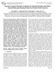
assignment problem. Fig. 3 summarize our approach to obtain the upper bound.
7.1. Static Demands Performance Bound
The static demands performance bound problem is as follows. A multichannel multi-radio WMN, which is modeled by a digraph, and a set of static
QoS demands are given. By the static demands, we mean all the demands arrive
at time 0. The question is what the maximum number of admissible demands is.
For this problem, we develop an optimal MILP model and since it is extremely
difficult, we relax it and obtain a relaxed model that is tremendously easier and
provides a tight bound for the problem.
7.1.1. Optimal Model
In the optimal MILP model, we use the assumptions we made in the previous sections; each link can only use one channel, there is not fast switching
capability, and the capacity constraint is modeled by the row constraint (1).
However, we assume that flows are splittable and multipath routing is used. In
addition to the notations in Table 1, we use the following variables. Binary
variable xk(u,v) is the channel assignment variable,
18
Static Demands
Assuming static
demands
Assuming fast
switching
Optimal model:
OPTIMALSTATIC
Relaxed model:
RELAXEDSTATIC
Time based constraints
and assuming rerouting
Dynamic Demands
Decomposition Algorithm:
MOSTGREEDYONLINE
Decomposition
Decomposable model:
DYNAMICUB2
Proposition 2
Upper bound model:
DYNAMICUB1
Performance Bound
Figure 3: The proposed approach to obtain network performance bound
xk(u,v)
(
1, if link (u, v) transmits on channel k
=
0, otherwise.
Binary variable ai denotes admission of demand δi ,
(
1, if demand δi is accepted
ai =
0, otherwise.
Tuning radios to channels is modeled by variable yuk ,
yuk = 1, if channel k is assigned to a radio of node u.
The optimal model is as follows. Its objective function is to maximize the
number of admitted demands,
X
maximize
ai .
(3)
δi ∈∆
Since at most one channel is assigned to each link, we have
X
xk(u,v) ≤ 1
∀(u, v) ∈ E.
(4)
k∈K
Obviously, the variable yuk cannot be greater than 1, so
yuk ≤ 1
∀k ∈ K, ∀u ∈ V.
(5)
If link (u, v) uses channel k, the channel must be assigned to a radio in both
nodes u and v, therefore
xk(u,v) ≤ yuk , xk(u,v) ≤ yvk
∀k ∈ K, ∀(u, v) ∈ E.
(6)
The radio constraint forces that the number of channels assigned to the links of
a node must be at most the number of radios of the node; in other words,
X
yvk ≤ rv
∀v ∈ V.
(7)
k∈K
19
If link (u, v) transmits a load on channel k, the channel must be assigned to the
link. So, we have
k
l(u,v)
≤ xk(u,v) ck(u,v)
∀k ∈ K, ∀(u, v) ∈ E.
(8)
The load transmitted by each link must be equal to the load offered on it by
flows in the network,
X
X
k
i
∀(u, v) ∈ E.
(9)
l(u,v)
=
f(u,v)
k∈K
δi ∈∆
Modeling the capacity constraint is a little complicated. To check the capacity constraint (1), I(u,v) and the channel assigned to (u, v) must be given, but
indeed these are determined after solving the optimization model. To deal with
′
this issue, in the optimization model, we use I(u,v)
instead of I(u,v) and check
′
the constraint for all channels, there are κ constraints per link. Recall that I(u,v)
is the interference set of (u, v) when a common channel is assigned to all links
in the network. However, only one of the κ constraints should be satisfied and
the remaining must be don’t-care because if channel k is not assigned to (u, v),
it is meaningless to impose a limitation on the aggregate load transmitted on
this channel in the interference range of the link. This is modeled using the big
M technique and the constraint is
X
k
l(a,b)
′
(a,b)∈I(u,v)
ck(a,b)
≤ 1 − xk(u,v) M + 1
∀k ∈ K, ∀(u, v) ∈ E.
(10)
In (10), if channel k is assigned to link (u, v), xk(u,v) = 1, the right-hand side
will be “1”, and the constraint imposes that the aggregate load transmitted
′
, on channel k must not
by the links in the interference rage of (u, v), I(u,v)
exceed physical channel capacities. However, for other channels k ′ 6= k where
′
xk(u,v) = 0, this constraint becomes don’t-care since M is a big value. The big
P
lk
lk
(a,b)
; since c(a,b)
≤1
value implies that M must be greater than (a,b)∈I ′
k
ck
(u,v)
(a,b)
(a,b)
′
ˆ we need M > I.
ˆ
and |I(u,v)
| ≤ I,
Finally, the routing and flow conservation constraint must be satisfied if
demand is accepted, which is modeled as
if u = si
ai b i ,
X
X
i
i
f(v,u) = −ai bi , if u = di
∀u ∈ V, ∀δi ∈ ∆. (11)
f(u,v) −
(v,u)∈E
(u,v)∈E
0,
otherwise
i
Note that routing variables f(u,v)
are real variables because of flow splitting and
multipath routing assumptions. The last constraints are the bounds,
k
i
xk(u,v) ∈ {0, 1}, ai ∈ {0, 1}, l(u,v)
≥ 0, f(u,v)
≥ 0, yuk ≥ 0.
(12)
Putting (3)–(12) altogether provides an optimal model for the static demands
performance bound problem that is
Model:
Objective:
Subject to:
OptimalStatic
(3)
(4)–(12).
20
Table 5: The number of maximal cliques
Node # Link # Interference Graph
Maximal Clique #
25
126
8
50
234
107
100
656
204
Whereas solving the OptimalStatic model gives an optimal feasible solution, it is extremely difficult. The model cannot be solved easily even for small
networks and a few number of demands. The complexity arises from the binary
variables xk(u,v) and ai . In the following, we deal with the complexity by relaxing
this optimal model.
7.1.2. Upper Bound
The binary variable xk(u,v) used for channel assignment is the source of the
difficulty of OptimalStatic. We assume that radios are capable to do fast
switching to tackle the complexity. Using this assumption, variable xk(u,v) is
relaxed as
xk(u,v) = Fraction of time that link (u, v) transmits on channel k.
However, this relaxation causes a problem. The capacity constraint (10)
is a conditional constraint and needs the binary variable xk(u,v) . We replace
it by the scaled clique constraint to deal with this issue. It enforces that the
aggregate load of the links in each maximal clique of the interference graph
should not exceed the scaled physical channel capacity. The clique constraint
P
lk
≤1
without scaling is a necessary condition4 and formulated as (u,v)∈Qi c(u,v)
k
(u,v)
in multi-rate networks [39], where Qi is a maximal clique. As shown in [38], to
be a sufficient condition, the constraint must be scaled.
There are two issues about the scaling. First, the number of maximal cliques
in an arbitrary graph theoretically can be exponential; but, in practice, in the
interference graph of multi-hop wireless networks, it is limited and all maximal
cliques can be found very easily. Table 5 shows the number of maximal cliques
in the interference graph of three random topologies. The maximum time to
find all maximal cliques is less than one second in our experiments on an Intel
Pentium IV 3.0 GHz machine5 .
Second, the value of the scale should be selected properly. The authors in
[38] showed that it depends on the imperfection ratio of the interference graph.
A recent simulation based study of the imperfection ratios of interference graphs
provided two conclusions [41]. First, as the number of nodes increases the value
of the scale decreases. Second, scale = 1.0 is a good approximation but to be
1
more conservative, we can use scale = 1.21
= 0.826. Based on this study, we
use both these values to find two bounds.
Let γ be the scale, Qi be a maximal clique in the interference graph when
a common channel is assigned to all links, and set Φ = {Q1 , Q2 , . . .} be the set
4 In
fact, it is a sufficient condition only in perfect interference graphs.
used MACE program to enumerate maximal cliques [40].
5 We
21
of the maximal cliques. The relaxed model for the static demands performance
bound problem is as follows.
Obviously, variable xk(u,v) is bounded by 1,
xk(u,v) ≤ 1
∀k ∈ K, ∀(u, v) ∈ E.
(13)
Load transmitted by link (u, v) on channel k is proportional to the fraction of
time that the link is active on the channel, so
k
l(u,v)
= xk(u,v) ck(u,v)
∀k ∈ K, ∀(u, v) ∈ E.
(14)
When a link of node u, either (u, v) or (v, u), uses channel k, xk(u,v) > 0, in fact,
a radio of the node is tuned to the channel and utilized for that transmission for
xk(u,v) fraction of time. Obviously, total utilization of radios of a node cannot
exceed the number of radios; in other words,
X X
X
xk(u,v) +
xk(v,u) ≤ ru
∀u ∈ V.
(15)
k∈K
(u,v)∈E
(v,u)∈E
The scaled clique constraint is
X
k
l(u,v)
ck
(u,v)∈Qi (u,v)
=
X
xk(u,v) ≤ γ
∀k ∈ K, ∀Qi ∈ Φ,
(16)
(u,v)∈Qi
that imposes the total time allocated to all conflicting links must be less than
or equal to γ. The bound constraints are
i
k
xk(u,v) ≥ 0, ai ∈ {0, 1}, l(u,v)
≥ 0.
≥ 0, f(u,v)
(17)
These constraints and objective function (3) gives the relaxed model as
Model:
Objective:
Subject to:
RelaxedStatic
(3)
(9), (11), (13)–(17).
It is important to note that even if the exact value of the scale is used,
this relaxed model will be an upper bound because its solution may not be
schedulable. An example of unschedulable solution is depicted in Fig. 4. In this
example, in the first time-slot, nodes a and b activate channel 1 on their radios
to transmit the load on link (a, b), the length of this time-slot is half of the
scheduling frame, x1(a,b) = 0.5, since the load on the link is 5 and the physical
channel capacity is 10. In the second time-slot, channel 2 is activated on the
radios of nodes b and c to transmit the load on link (b, c), the length of this
time-slot is also half of the scheduling frame, x2(b,c) = 0.5. However, there is
not any time-slot to transmit the load on link (c, a) on channel 3 even though
all the constraints of the RelaxedStatic model are satisfied. Our simulation
results presented in the next subsection show that this issue is not an important
matter and RelaxedStatic provides a tight bound.
22
1 -
1 2
a
b
(1,5)
)
(2
,5
)
,5
(3
c
- 2
Figure 4: An example of unschedulable solution. Label of each link is (channel, load), label of
each node is the schedule of channel activation on its radio, ck(u,v) = 10, and qu = 1. Whereas
all the constraints of RelaxedStatic are satisfied, there is not any feasible schedule.
Parameter
Name
Area
Node #
TR
IR
Radio #
Channel #
ck(u,v)
Table 6: Parameters of the topologies used in simulations
Values
T-10
T-15
T-25
T-50
500×500m2
600×600m2
750×750m2
1000 × 1000m2
10
15
25
50
200m
200m
200m
200m
400m
400m
400m
400m
Random [2,5] Random [2,5] Random [2,5]
Random [2,5]
12
12
12
12
100 Mb/s
100 Mb/s
100 Mb/s
100 Mb/s
7.1.3. Simulation Results
In this subsection, we present simulation results to show the efficiency and
tightness of the RelaxedStatic model. We conducted the simulations in three
10, 15, and 25 nodes random topologies with parameters shown in Table 6. In
each experiment, 50 random demands were offered to the network. The required
bandwidth of each demand was a uniform random variable in [1, Bmax ] Mb/s.
We used CPLEX 11.0 [42] on an Intel Pentium IV 3.0GHz machine with 2 Gigabytes RAM. Time limit to solve the model was 10 hours. The results presented
in this section are the average of five experiments. We evaluate RelaxedStatic
using following metrics.
Definition 4. Bound Gap of the relaxed model is
Relaxed Model Accepted Demands # − Optimal Model Accepted Demands #
.
Optimal Model Accepted Demands #
Definition 5. Time Ratio of the relaxed model is
Optimal Model Solution Time
Relaxed Model Solution Time .
Table 7 shows the simulation results. In this table, rows “Optimal,” “Not
Scaled,” and “Scaled” are the results of OptimalStatic and RelaxedStatic
with γ = 1.0 and γ = 0.826, respectively. The “Exceed #” row is the number
of times that OptimalStatic was not solved in the specified time limit, in
these cases, we used the best integer solution as the result. Optimality gap of
the best integer solution, which is reported by the solver, is represented in the
“Optimality Gap” row.
23
Table 7: Simulation results of OptimalStatic and RelaxedStatic. The parameters of the
simulation topologies are shown in Table 6.
Topology
T-10
T-15
T-25
Bmax
20
30
20
30
20
30
Optimal
48.8
44
49.4
44.4
46.6
40
Accepted # Not Scaled
49.3
45.4
49.4
45
49.9
44.8
Scaled
48.5
42.8
48.8
42.6
48.8
42
Bound Gap
Not Scaled
1.09e−2
3.13e−2
0
1.35e−2
7.09e−2
1.20e−1
Scaled
−6.15e−3
−2.84e−2
−1.21e−2
−4.05e−2
4.68e−2
5.00e−2
Optimal
2.17e+4
3.60e+4
1.09e+4
3.60e+4
3.60e+4
3.60e+4
Time(sec)
Not Scaled
9.50e−2
1.73e−1
4.74e−1
6.24e−1
8.71e−1
3.38e+0
Scaled
1.20e−1
1.12e−1
4.62e−1
8.90e−1
2.16e+0
5.71e+0
Time Ratio
Not Scaled
2.28e+5
2.08e+5
2.30e+4
5.77e+4
4.13e+4
1.07e+4
Scaled
1.81e+5
3.22e+5
2.36e+4
4.04e+4
1.67e+4
6.31e+3
Exceed #
2
5
1
5
5
5
Optimality Gap
1.66e−2
1.13e−1
6.38e−2
1.27e−1
7.46e−2
2.08e−1
These results lead to the following conclusions. First, RelaxedStatic is
a tight relaxation of the optimal model as the bound gap is very small. Second, RelaxedStatic is incredibly, up to 3.22e+5 times, faster than OptimalStatic. Third, the best integer solution is a fairly good approximation of
the optimal solution since the optimality gap is quite small. Fourth, these results confirm the conclusions in [41]: (i) γ = 0.826 is too conservative for small
topologies as the bound gap is negative in T-10 and T-15. (ii) As the number
of nodes increases, γ = 1.0 and γ = 0.826 get looser and tighter, respectively.
7.2. Dynamic Demands Performance Bound
Dynamic demands performance bound problem is, in fact, the performance
bound of the joint QoS routing and channel assignment problem in which each
demand δi arrives at time ti and has a limited holding time ei − ti . Again,
the question is the maximum number of admissible demands. As explained
before, for the problem, we first develop an upper bound model by extending
RelaxedStatic; then, propose another model, which is equivalent to the first
one and is decomposable; finally, we develop a decomposition algorithm that
divides the second model into subproblems and solves them sequentially.
7.2.1. Upper Bound Model
As mentioned, in this problem, we should model the dynamics of the demands, which need to update network configurations (routing and channel assignment) at the demand arrival times. We deal with the problem by extending
RelaxedStatic in the following ways. First, we introduce a time set T , which
is T = {t1 , t2 , . . . , th }, and duplicate the channel assignment variables, xk(u,v) , for
each tj ∈ T , i.e., we add new variables xk(u,v),tj ∀k ∈ K, ∀(u, v) ∈ E, ∀tj ∈ T .
Second, we assume that accepted demands can be rerouted ; thus, flow routes
are time-dependent and reoptimized at each demand arrival time. They are
i
∀δi ∈ ∆, ∀(u, v) ∈ E, ∀tj ∈ T . Third, decision variable ai
denoted by f(u,v),t
j
is not duplicated because a demand is either accepted or not independent of the
time we observe the network. Fourth, the required bandwidth of demand δi is
defined as
24
bi,tj =
(
bi , if ti ≤ tj ≤ ei
0, otherwise.
These extensions yield a model that is composed of h instances of the RelaxedStatic model, an instance per demand arrival. At each arrival time
tj ∈ T , decision variables must satisfy the constraints of the instance of RelaxedStatic corresponds to the time, which are defined as following.
Definition 6. Constraints must be satisfied at time tj , ConsSet(tj ), are
xk(u,v),tj ≤ 1
∀k ∈ K, ∀(u, v) ∈ E,
k
∀k ∈ K, ∀(u, v) ∈ E,
= xk(u,v),tj ck(u,v)
l(u,v),t
j
X
X
X
∀v ∈ V,
xk(v,u),tj ≤ rv
xk(u,v),tj +
k∈K
X
(u,v)∈Qi
(v,u)∈E
(u,v)∈E
k
l(u,v),t
j
ck(u,v)
X
=
(u,v)∈E
and
i
f(u,v),t
j
−
X
(v,u)∈E
xk(u,v),tj ≤ γ
∀k ∈ K, ∀Qi ∈ Φ,
(u,v)∈Qi
i
f(u,v),t
=
j
δi ∈∆
X
X
X
k
l(u,v),t
j
∀(u, v) ∈ E,
k∈K
i
f(v,u),t
j
ai bi,tj ,
= −ai bi,tj ,
0,
if u = si
if u = di ∀u ∈ V, ∀δi ∈ ∆,
otherwise
(18)
i
k
≥ 0.
≥ 0, f(u,v),t
xk(u,v),tj ≥ 0, ai ∈ {0, 1}, l(u,v),t
j
j
The major complexity of this model is that these instances are not independent because variables ai ∀δi ∈ ∆ appear in all of them. In other words,
demands are not preemptable; if a demand is accepted in the solution of one of
the instances, it must be accepted in the remaining. As a result, we have to
solve the h instances altogether simultaneously.
An important issue in modeling the dynamic demands performance problem,
which needs to be addressed carefully, is the objective function of the model. If
(3) is optimized, this model will be an appropriate model for the off-line joint
QoS routing and channel assignment problem, in which the information about
all demands is given at the beginning and solving the model finds the maximum
number of admissible demands. However, in this paper, we have focused on
the on-line greedy CAC strategy, where the information about a demand is
not known before its arrival time and at demand arrival time, since the on-line
algorithm does not aware of future demands, it greedily attempts to accept the
given demand. We borrow the idea proposed in [43] to model this behavior of
on-line algorithms, which is assigning profit ρi to demand δi and maximizing
the aggregate profit of accepted demands. Suppose ∆ is sorted in ascending
order of ti , the profit is assigned as
ρi = 2h−i .
25
(19)
and the objective function is
maximize
X
a i ρi .
(20)
δi ∈∆
These profits imply that if there is a feasible path for demand δiP
, it is not
h
rejected in favor of accepting subsequent demands δj because ρi > j=i+1 ρj
∀δi ∈ ∆. This inequality implies that the model first puts its effort to accept δ1 ,
then consider δ2 , after that, δ3 and so on; this exactly simulates the behavior of
on-line greedy CAC algorithms.
The optimization model for the dynamic demands performance problem is
Model:
Objective:
Subject to:
DynamicUB1(∆, ρ)
(20)
ConsSet(tj ) ∀tj ∈ T .
Where ρ is the profit assignment vector obtained by (19). Since instead of OptimalStatic, we use the RelaxedStatic model, DynamicUB1 provides an
upper bound on the network performance achievable through on-line greedy algorithms. Tightness of the model depends on the scale used in RelaxedStatic
and as discussed in the previous subsection, in large networks, scale 0.826 yields
a tighter bound than scaled 1.0.
There is a problem about DynamicUB1, this model will be huge even for
medium size networks and a large number of demands; it is not solvable for
practical networks. In the following, we decompose it to deal with this issue.
7.2.2. Decomposition
In this subsection, at the first step, we define a model that is equivalent
to DynamicUB1, the set of accepted demands is the same for both models.
Then, in the second step, we show this model is decomposable and develop an
algorithm to decompose it.
The decomposable model is obtained through following modifications in DynamicUB1. First, instead of ai for each demand we consider ai,tj for each
demand δi and tj ∈ T . Second, we consider two additional constraints
∀δi ∈ ∆, ∀tj ∈ T,
ai,tj ≤ bi,tj M
−1
where M > min{bi }
and
∀δi ∈ ∆, ∀tj ∈ T.
ai,tj ≤ ai,ti
(21)
(22)
Constraints (21) and (22) impose that ai,tj must be zero if bi,tj = 0 or ai,ti = 0,
respectively. Third, profit assignment is
0, tj < ti
ρi,tj = 1, tj = ti
∀δi ∈ ∆, ∀tj ∈ T.
(23)
2, tj > ti .
Fourth, the new objective function is
X X
maximize
ai,tj ρi,tj .
tj ∈T δi ∈∆
Consequently, the decomposable model is
26
(24)
Model:
Objective:
Subject to:
DynamicUB2(∆, ρ)
(24)
(21), (22), and ConsSet′ (tj ) ∀tj ∈ T .
Where ConsSet′ (tj ) is the same set of constraints denoted by ConsSet(tj )
but ai is replaced by ai,tj and ρ is the profit assignment vector obtained by
(23).
We use following propositions to show that DynamicUB1 and DynamicUB2 are equivalent models.
Proposition 1. In the solution of DynamicUB2, we have ai,ti = ai,tj where
ti ≤ tj ≤ e i .
Proof. The proof can be found in the Appendix.
Proposition 2. For a given ∆, we have ai = ai,ti , where ai and ai,ti are
obtained by solving the DynamicUB1 and DynamicUB2 models, respectively.
Proof. The proof can be found in the Appendix.
In DynamicUB1, the accepted demands are determined by ai , demand δi
is accepted if ai = 1; now, if we define it in DynamicUB2 using ai,ti , demand
δi is accepted if ai,ti = 1, the set of accepted demands obtained by both models
are the same due to proposition 2; in other words, these models are equivalent.
The distinguishing feature of the DynamicUB2 model is that we can decompose it into h subproblems and solve them sequentially. Note that constraint
ConsSet′ (tj ) ∀tj ∈ T in the model is indeed h independent sets of constraints,
there is not any common variable among them. Each set contains the decision
variables, and constraints correspond to a tj ∈ T . Therefore, DynamicUB2
can be decomposed into h subproblems where jth subproblem is
Model:
Objective:
Subject to:
subUB2(∆′tj , ρ, j)
P
maximize δi ∈∆′ ai,tj ρi,tj
tj
ConsSet′ (tj ).
In this model, constraints (21) and (22) are not included, we take them into
/ ∆′tj if either of these
account using ∆′tj ⊂ ∆ instead of ∆. Demand δi ∈
conditions holds
• tj < ti or tj > ei since bi,tj = 0 and constraint (21) implies ai,tj = 0.
• ti < tj ≤ ei and ai,ti = 0 because constraint (22) enforces ai,tj = 0.
Since when ti < tj ≤ ei , constraint (21) does not impose any restriction, the
first condition is equivalent to the constraint. In a similar way, the second
condition is equivalent to (22) as the constraint is don’t-care when ai,ti = 1.
Therefore, subUB2 is a valid decomposition of DynamicUB2 as it takes all
the constraints of DynamicUB2 into consideration.
Note that the second condition needs the optimal value of ai,ti ; it implies that
subUB2(∆′ti , ρ, i) must be solved before subUB2(∆′tj , ρ, j) for each j > i; in
other words, subUB2 subproblems should be solved sequentially starting from
subUB2(∆′t1 , ρ, 1). This is implemented by the decomposition algorithm as
shown in algorithm 6. In this algorithm, if δi is rejected, it is removed from ∆′
27
Algorithm 6 : MostGreedyOnline(∆)
1: Create empty set ∆′
2: for i = 1 to h do
3:
δi ← ∆[i]
4:
Add δi to ∆′
5:
Assign profits ρ according (23)
6:
Solve subUB2(∆′ , ρ, i)
7:
if ai,ti = 1 then
8:
Add δi to the Accepted demand set
9:
else
10:
Remove δi from ∆′
11:
for each δj ∈ ∆′ do
12:
if ej < ti+1 then
13:
Remove δj from ∆′
in line 10, due to (22); moreover, it is removed in line 13 because of (21) if it
does not overlap with the next demand.
This algorithm is named “most greedy on-line” since it is on-line, it does not
use the information of a demand before it arrives, and is the greediest algorithm;
it accepts demands if there is a feasible network configuration, which is checked
by solving the subUB2 optimization model.
8. Simulation Results
In this section, we present simulation results to evaluate the performance
of the JQRCA algorithm. After clarifying the simulation setup and simulated
algorithms, we study the effect of different parameters on the performance of
the algorithms. Moreover, we present results on the average case computational
complexity and overhead of the JQRCA algorithm.
8.1. Simulation Setup
We used a flow-level event-driven simulator developed in Java. Simulations
were performed on an Intel Pentium IV 3.0 GHz machine with 2 Gigabytes RAM
and CPLEX 11.0 was used. Three random topologies with 15, 25, and 50 nodes
as shown in Table 6 were used. In each run of the simulations, a set of random
traffic demands with the parameters shown in Table 8 was used. These were the
default values used in all simulations, unless otherwise is stated. The simulation
parameters, e.g., λ, Bmax , and κ, were tuned to consider the networks under
lightly loaded to highly overloaded conditions. The results presented in this
section are the average obtained from ten different demand sets.
We simulated three solutions for the on-line joint QoS routing and channel
assignment problem: the JQRCA algorithm, the MostGreedyOnline algorithm, and a static solution. In the static solution, at the beginning, we assign
channels by the minimum interference greedy channel assignment algorithm
[44], which is a static channel assignment to minimize total network interference, then, route flows using the minimum hop count routing. In the following
figures, “MGO-0.82,” “MGO-1.00,” “JQRCA,” and “Static” are the results of
28
Table 8: Parameters of simulation traffic
Parameter
Value
Number of demands (h)
300
Arrival rate
Poisson random variable with mean λ demands per min.
Holding time (µ−1
= ei − ti )
Exponential random variable with mean 10 min.
i
Required bandwidth (bi )
Uniform random variable in [1, Bmax ] Mb/s
Table 9: The correspondence between demand arrival rate, incoming traffic, and overload
percentage
λ
Incoming
Overload %
(demand/min)
Traffic (Mb/s)
T-15
T-25 T-50
2
210
22
18
15
4
420
44
36
30
6
630
66
54
45
8
840
88
72
60
10
1050
110
90
75
MostGreeyOnline with γ = 0.826, MostGreeyOnline with γ = 1.0, the
JQRCA algorithm with k = 2, and the static solution, respectively.
In the following results, we report the incoming traffic in terms of demand
arrival rate. The incoming traffic can also be easily measured in terms of bandwidth as follows. The average holding time of demands is µ−1 minutes and λ
new demands arrive in each minute; thus, using the Little’s law, there are λµ−1
traffic demands on average. Since the bandwidth requirement of demands is a
+1
uniform random variable in [1, Bmax ] Mb/s, its average value is Bmax
Mb/s.
2
Therefore, the total traffic offered to the network in terms of bandwidth is
0.5λµ−1 (Bmax + 1) Mb/s. Table 9 shows the correspondence between demand
arrival rate and incoming traffic. Moreover, this table shows the overload percentage of each topology per arrival rate. The overload percentage is the percentage of the incoming traffic over the maximum throughput of the network.
The maximum throughput of the network is measured as follows. We load the
network very heavily, e.g., λ = 1000 demand/min, use the MGO-1.00 to route
the demands, and take the moving average of the bandwidth of the accepted
demands over the time. The maximum throughput of the T-15, T-25, and T-50
topologies are 995 Mb/s, 1170 Mb/s, and 1394 Mb/s, respectively.
To measure the performance of QoS routing algorithms, we use the demand
acceptance rate metric [11, 45]. Demand acceptance rate is the number accepted
demands divided by the total number of demands. We discuss the relation
between bandwidth of accepted demand and this metric, which depends on the
fairness of the algorithm, in subsection 8.6.
8.2. Effect of Demand Arrival Rate
Arrival rate of demands is the first parameter we investigated. The acceptance rates of the solutions versus the demand arrival rate are shown in Fig. 5.
These figures show that the JQRCA algorithm is an efficient algorithm, it significantly outperforms the static solution and has a comparable performance
to the bound obtained by the MostGreedyOnline algorithm independent of
the size of the network. As we see, in the worst case, the solution obtained by
JQRCA is not far from the solution of MGO-0.82 more than 6–8%.
29
In Fig. 6, we depict the average solution time per subUB2 subproblem
to show the efficiency of the MostGreedyOnline algorithm. This problem
is solved by the algorithm at the arrival time of each demand. This figure
shows that the algorithm is not time-consuming as the solution time is less
than 0.6 second, 1.2 second, 12 second in the T-15, T-25, and T-50 topologies,
respectively.
8.3. Effect of Maximum Required Bandwidth
The maximum required bandwidth, Bmax , is a parameter influencing the
offered load; hence, the performance of the algorithms depends on it. The
acceptance rates of the algorithms versus the maximum required bandwidth
are depicted in Fig. 7. These results show that acceptance rate is a decreasing
function of Bmax but the rate of reduction for JQRCA is much less than the
Static solution and is comparable to the rate of MGO-0.82. As seen in the
figures, the gap between the acceptance rates of JQRCA and MGO-0.82 enlarges
as Bmax increases; this is due to the flow-splitting and multipath routing. A
flows that needs large amount of bandwidth is split into multiple sub-flows by
the MostGreedyOnline algorithm, which are routed through multiple paths;
however, the JQRCA algorithm is not allowed to split flows and cannot find a
feasible path for the bandwidth intensive flows.
8.4. Effect of Number of Available Channels
An efficient joint QoS routing and channel assignment algorithm should be
able to exploit available channels. We conducted simulations with different
numbers of channels in order to compare the algorithms from this point of view.
In these simulations, λ is 4 demands per minute that leads to 420 Mb/s offered
load. Fig. 8 shows the performance of the algorithms versus the number of
available channels. In all topologies, JQRCA exploits the available channels
as well as the MostGreedyOnline algorithm since the rate of increasing of
acceptance rate is almost the same for both algorithms. In the T-15 topology,
Fig. 8(a), JQRCA outperforms MGO-0.82, this confirms our previous results in
Section 7.1.3 that showed the scale 0.826 is too conservative in small topologies.
8.5. Effect of Number of Radios per Node
Radios in each node are scarce resources. An efficient algorithm should be
capable of providing good performance even using a limited number of radios.
We show the performance of the algorithm versus the numbers of radios per
node in Fig. 9. These figures show that JQRCA does not need many radios per
node to achieve high network performance.
When there are two or three radios per node, there is a large gap between
JQRCA and MGO-0.82. This is due to the infeasibility of the solutions of the
subUB2 model, which is explained in Section 7.1.2. The unschedulability issue
is more serious when ru is small; so, in this case the MostGreedyOnline
algorithm gives a bit loose upper bound on the network performance.
Fig. 8 and Fig. 9 indicate the main factor limiting the network performance
is the number channel not the number of radios. In real-life WMNs, in which
each node has three/four radios, JQRCA can exploit the many existing channels,
e.g., 12 orthogonal channels in IEEE 802.11a, to obtain a near optimal network
performance.
30
1
MGO−1.00
MGO−0.82
JQRCA
Static
Acceptance Rate
0.9
0.8
0.7
0.6
0.5
2
4
6
Arrival Rate (demand / min)
8
10
(a) T-15 Topology
1
MGO−1.00
MGO−0.82
JQRCA
Static
0.9
Acceptance Rate
0.8
0.7
0.6
0.5
0.4
0.3
2
4
6
Arrival Rate (demand / min)
8
10
(b) T-25 Topology
1
MGO−1.00
MGO−0.82
JQRCA
Static
0.9
Acceptance Rate
0.8
0.7
0.6
0.5
2
4
6
Arrival Rate (demand / min)
8
10
(c) T-50 Topology
Figure 5: Acceptance rate versus demand arrival rate. The parameters of the topologies and
the simulation traffic are shown in tables 6 and 8, respectively; and Bmax = 20.
31
0.6
MGO−0.82
MGO−1.00
Subproblem Solution Time (sec)
0.5
0.4
0.3
0.2
0.1
0
2
4
6
Arrival Rate (demand / min)
8
10
8
10
8
10
(a) T-15 Topology
1.2
MGO−0.82
MGO−1.00
Subproblem Solution Time (sec)
1
0.8
0.6
0.4
0.2
0
2
4
6
Arrival Rate (demand / min)
(b) T-25 Topology
12
MGO−0.82
MGO−1.00
Subproblem Solution Time (sec)
10
8
6
4
2
0
2
4
6
Arrival Rate (demand / min)
(c) T-50 Topology
Figure 6: Average solution time of subUB2 versus demand arrival rate. The parameters of the
topologies and the simulation traffic are shown in tables 6 and 8, respectively; and Bmax = 20.
32
1
Acceptance Rate
0.9
0.8
0.7
MGO−1.00
MGO−0.82
JQRCA
Static
0.6
10
15
20
Bmax
25
30
25
30
25
30
(a) T-15 Topology
1
0.9
Acceptance Rate
0.8
0.7
0.6
0.5
MGO−1.00
MGO−0.82
JQRCA
Static
0.4
10
15
20
Bmax
(b) T-25 Topology
1
Acceptance Rate
0.9
0.8
0.7
0.6
0.5
10
MGO−1.00
MGO−0.82
JQRCA
Static
15
20
Bmax
(c) T-50 Topology
Figure 7: Acceptance rate versus the maximum required bandwidth. The parameters of the
topologies and the simulation traffic are shown in tables 6 and 8, respectively; and λ = 4
demands per minutes.
33
1
MGO−1.00
MGO−0.82
JQRCA
Static
Acceptance Rate
0.9
0.8
0.7
0.6
0.5
4
6
8
# of Channels
10
12
10
12
10
12
(a) T-15 Topology
1
MGO−1.00
MGO−0.82
JQRCA
Static
0.9
Acceptance Rate
0.8
0.7
0.6
0.5
0.4
4
6
8
# of Channels
(b) T-25 Topology
1
MGO−1.00
MGO−0.82
JQRCA
Static
0.9
Acceptance Rate
0.8
0.7
0.6
0.5
0.4
4
6
8
# of Channels
(c) T-50 Topology
Figure 8: Acceptance rate versus the number of channels. The parameters of the topologies
and the simulation traffic are shown in tables 6 and 8, respectively. λ = 4 demands per minute
and Bmax = 20.
34
1
0.9
Acceptance Rate
0.8
0.7
0.6
MGO−1.00
MGO−0.82
JQRCA
Static
0.5
0.4
2
3
4
# of Radios per Node
5
6
(a) T-15 Topology
1
0.9
Acceptance Rate
0.8
0.7
0.6
MGO−1.00
MGO−0.82
JQRCA
Static
0.5
0.4
2
3
4
# of Radios per Node
5
6
(b) T-25 Topology
1
0.9
Acceptance Rate
0.8
0.7
0.6
0.5
MGO−1.00
MGO−0.82
JQRCA
Static
0.4
0.3
2
3
4
# of Radios per Node
5
6
(c) T-50 Topology
Figure 9: Acceptance rate versus the number of radios per node. The parameters of the
topologies and the simulation traffic are shown in tables 6 and 8, respectively. λ = 4 demands
per minute and Bmax = 20.
35
8.6. Fairness
As mentioned in Section 3.5, greedy CAC strategy is suitable to achieve
(absolute) fairness. In this subsection, we measure the fairness of the JQRCA
algorithm through the Jain’s fairness index [46]. Suppose there are N traffic
classes and Ai demands are accepted from class i. Fairness index is defined as
Fairness index =
P
N
N
i=1
PN
Ai
i=i
2
A2i
.
This parameter measures how fairly an algorithm accepts demands from
different classes. Absolute fairness is achieved when the fairness index is equal
to one, which implies the same number of demands is accepted from all classes;
absolute unfairness, when all the accepted demands belong to only one class, is
the case that fairness index is N1 .
Here, we define traffic classes based on the bandwidth requirements; we
divide [1, Bmax ] into 10 subintervals. Demand δi is in class j if (bi − 1) ∈
Bmax
[(j − 1) Bmax
10 , j 10 ] Mb/s. The fairness index of JQRCA in various settings of
network and traffic parameters is shown in Table 10. Note that these parameter
settings are the values we used in the previous subsections. This table shows that
JQRCA is quite fair, fairness index is more than 0.90 in most cases even when
acceptance rate is about 0.6. These results confirm the intuition; since JQRCA
attempts to accept every demand regardless of its bandwidth requirement, it
achieves the absolute fairness in lightly or moderately loaded networks.
These results can be used to compute network throughput in terms of bandwidth. Let us denote the acceptance rate, average bandwidth requirement of
accepted demands, and fairness index by α, b and η, respectively. The rate of
admitted demands is αλ demand per minute. According to the Little’s law, the
average number of demands active in the network is αλµ−1 . Consequently, the
network throughput is αλµ−1 b Mb/s. If JQRCA was absolutely fair, η = 1, it
would accept exactly the same number of demands from each class and thus
+1
. However, JQRCA is a bit unfair in some cases. In these cases,
b = Bmax
2
Bmax +1
b <
because the acceptance probability of the demands with small
2
bandwidth requirements is more than the probability of demands that need
large bandwidth. We take this observation into account through scaling down
b by the fairness index; we approximate the network throughput as
Approximated Throughput = 0.5αλµ−1 η σ (Bmax + 1)Mb/s,
where σ is a parameter to control the scaling. Our simulations show that this
approximation is very accurate. In Table 10, column “Throughput” is the actual network throughput measured from the simulations. The last column in
this table represents the throughput approximation normalized error. It is obtained by computing the difference between the actual network throughput and
the approximated throughput and then dividing the difference by the actual
throughput. We used σ = 2 in our simulations and as seen in the table, the
error is almost less than 2.5%.
8.7. Complexity and Overhead
In subsections 5.4 and 6.4, we analyzed the worst case complexity of the
QDDCA and JQRCA algorithms. In this section, we provide an insight into the
36
Table 10: Fairness index of JQRCA and throughput approximation normalized error.
Configuration
Throughput Acceptance Fairness Approx.
Topology
λ
Bmax
κ
ru
(Mb/s)
Rate
Index
Error %
T-50
4
20
12
Random
347.94
0.858
0.990
2.1
T-25
4
20
12
Random
347.97
0.861
0.990
2.0
T-15
10
20
12
Random
568.81
0.646
0.922
1.9
T-50
10
20
12
Random
537.80
0.615
0.918
1.7
T-25
4
10
12
Random
220.19
0.992
0.998
1.9
T-15
4
10
12
Random
220.31
0.998
0.999
2.0
T-50
4
30
12
Random
412.12
0.736
0.963
2.9
T-25
4
30
12
Random
400.42
0.721
0.955
2.2
T-15
4
20
4
Random
211.34
0.603
0.907
2.2
T-50
4
20
4
Random
166.01
0.506
0.858
5.1
T-50
4
20
12
3
346.41
0.853
0.983
1.8
T-25
4
20
12
3
360.64
0.882
0.993
1.5
T-15
4
20
12
6
403.52
0.990
0.999
1.5
T-50
4
20
12
6
377.06
0.919
0.995
1.6
average case complexity and overhead of the algorithms through simulations.
The computational complexity of JQRCA is proportional to the number of
violated links, which are generated during the search for a feasible path, and
the average number of calls of LinkChannelChange to resolve a violated link.
These statistics are presented in Table 11. In this table, column “Zero” refers
to the violated links that are assigned to the virtual channel 0 and column
“Non-Zero” are the remaining. When demand arrival rate is low, e.g., λ = 2,
a large percentage of the violated links, e.g., 89% in T-15 or 91% in T-50, are
the links on channel 0; because in this case, there are very few flows in the
network and consequently, many links are assigned to the virtual channel since
no load is on them. On the other hand, in high demand arrival rates, e.g.,
λ = 10, there are many flows in the network and a large number of links are assigned to a non-zero channel; therefore, a small percentage of the violated links,
e.g., 19% in T-25 or 26% in T-50, are on channel 0. Table 11 also shows that
LinkChannelChange is called more than one time per violated link. This
is because GroupChannelChange generates new violations that LinkChannelChange is called for them too. However, this extra complexity is not more
than one additional LinkChannelChange call, which is much less than what
ˆ
we considered in the worst case complexity analysis, I.
After finding a feasible path, network is updated through messages sent
from the call admission control server to the nodes in the network; the update
includes the path establishment and updating channel assignment. The messaging overhead of the former and latter updates are respectively proportional
to the average path hop count and the number of channel updates per accepted
demand, which are reported in Table 12. It is seen that the number channel
updates depends on the topology and the path hop count is much less than
n. It is important to note that the overhead caused by the dynamic channel
reassignment is not significant in comparison to the overhead of QoS routing;
in fact, in the worst case, λ = 8 in T-50, the overhead of channel reassignment
is less than 53% of the overhead of routing.
Tables 11 and 12 show that the complexity and overhead of the JQRCA
algorithm in practice are much less than the worst case presented in Sections
5.4 and 6.4; we believe the algorithm is an efficient solution for real-life WMNs.
37
Table 11: Average case computational complexity of the JQRCA algorithm. The parameters
of the simulation topologies and traffic are shown in tables 6 and 8, respectively. Bmax = 20
and k = 2.
Violations per Demand
LinkChannelChange
λ
Zero
Non-Zero
Call per Violation
T-15
T-25
T-50
T-15
T-25 T-50
T-15
T-25
T-50
2
0.87
1.24
1.88
0.10
0.22
0.17
1.03
1.04
1.019
4
0.57
0.88
1.38
0.68
1.15
1.13
1.44
1.19
1.40
6
0.46
0.78
1.21
1.34
1.84
1.75
1.56
1.26
1.51
8
0.43
0.71
1.189
1.84
2.41
2.82
1.70
1.27
1.68
10
0.40
0.68
1.11
2.26
2.79
3.06
1.84
1.33
1.73
Table 12: Overhead of the JQRCA algorithm. The parameters of the simulation topologies
and traffic are shown in tables 6 and 8, respectively. Bmax = 20 and k = 2.
Channel Updates per
Path Hop Count
λ
Accepted Demand
T-15
T-25
T-50
T-15
T-25
T-50
2
0.882
1.303
1.990
2.096
2.871
4.090
4
0.828
1.106
1.850
2.053
2.814
4.023
6
0.848
1.086
1.942
2.021
2.832
3.952
8
0.891
1.108
2.040
2.001
2.747
3.871
10
0.882
1.072
1.933
1.922
2.696
3.840
9. Conclusions and Future Work
We studied the problem of performance optimization of multi-channel multiradio WMNs in presence of traffic with QoS constraints, which is measured in
terms of acceptance rate of traffic demands. To boost the network performance,
we proposed an on-line joint QoS routing and channel (re)assignment algorithm
that utilizes network resources efficiently by optimal routing and adapts them
through appropriate channel reassignments. The algorithm does not require
any prior information about the offered load, and aims to keep the number of
channel reassignments small. At demand arrival times, the algorithm finds a
path, if it is not feasible, it detects the violated links and attempts to resolve
them. If all the violations are not resolved, another path is found, and so on.
The algorithm examines up to k paths.
We approached the problem of finding an upper bound on the maximum
number of admissible demands by formulating it as a MILP model and developing a decomposition algorithm for the model. It is important to note that the decomposition technique can be used for other similar problems e.g., performance
bound of dynamic QoS routing in wired networks. Comparing the JQRCA algorithm to the bound obtained by the decomposition algorithm shows that in
spite of the fact that JQRCA is not allowed to reroute existing flows, cannot
use the flow splitting and multipath routing mechanisms, and is restricted to
change only the channels in range 2IR of flow routes, its performance is near to
the bound in different network and traffic parameter settings. It can efficiently
exploit available channels even with very few radios per node.
In this paper, we considered greedy CAC strategy, assumed perfect orthogonal channels, and proposed a centralized algorithm. We plan to develop a
distributed version of JQRCA and extend it to consider non-greedy CAC mechanisms and adjacent channel interferences in the future. Moreover, routing metrics other than |I(u,v) |, e.g., hop-count bounded widest path, can be considered
38
in the future work.
10. Acknowledgment
We would like to thank the reviewers for their helpful comments.
Appendix A. Proof of Proposition 1 and 2
In the DynamicUB2 model, let Xtj be a set contains demand δj and active
demands at time tj , demands that ai,tj−1 = 1 and bi,tj 6= 0. Let Ytj ⊆ Xtj be
the set of demands that satisfy ConsSet′ (tj ), and let Ztj ⊂ Ytj be the set of
demands that leave the network before tj+1 .
We prove proposition 1 as follows.
Proof. If ai,ti = 0, constraint (22) enforces that ai,tj = ai,ti = 0 ∀ti ≤ tj ≤ ei .
In the case of ai,ti = 1, we prove it by induction.
Base case: If j = i + 1, then we have Xtj = Yti ∪ δj \ Ztj . For the sake of
simplicity of presentation, we assume Ztj = ∅, the proof is in a similar way when
Ztj 6= ∅. If there is a feasible network configuration to accept all demands belong
to Xtj , we have ai,tj = 1, thus ai,ti = ai,tj = 1. Otherwise, if all the demands
cannot be accepted, δj must be rejected because ρj,tj < ρi,tj ∀δi ∈ Xtj \ δj .
Rejecting δj is sufficient since there is a feasible configuration for Xtj \ δj = Ytj ,
thus in this case, also, ai,ti = ai,tj = 1.
Induction step: Suppose j > i + 1. If ei > tj , demand δi is an active
demand, δi ∈ Xtj . According to the induction assumption, we have ai,tj−1 = 1.
Similar to the discussion about the base case, if all demands belong Xtj are
accepted, Xtj = Ytj , we have ai,tj = ai,tj−1 = ai,ti = 1; otherwise, again δj
must be rejected, and it is sufficient since there is a feasible configuration for
Ytj−1 ; therefore, again we have ai,tj = ai,tj−1 = ai,ti = 1 that completes the
proof.
The proof of proposition 2 is as follows.
Proof. We prove it by induction which is based on the number of demands, h.
Base case: When h = 1, ∆ = {δ1 }, both DynamicUB1 and DynamicUB2
models are the same and if there is a feasible path for the demand, it is accepted,
a1 = a1,t1 = 1, otherwise it is rejected, a1 = a1,t1 = 0.
Induction step: Suppose ai = ai,ti for i = 1, . . . , h when h = j −1. Increasing
the number of demands to h = j has two effects:
• It adds new constraint (18) corresponds to each δj to ConsSet(ti ) and
ConsSet′ (ti ) where i = 1, . . . , j − 1.
• It adds a new set of variables and constraints to both models, which
are denoted by ConsSet(tj ) and ConsSet′ (tj ) in DynamicUB1 and
DynamicUB2, respectively.
We make the following observations
1. We neglect the first effect because for i = 1, . . . , j −1, we have bj,ti = 0 and
therefore, the right-hand side of (18) is 0 and the constraint is don’t-care.
39
2. Adding ConsSet(tj ) to DynamicUB1 does not affect the optimal value
of ai for i = 1, . . . , j − 1 since ρi > ρj .
3. Adding ConsSet′ (tj ) to DynamicUB2 does not affect the optimal value
of ai,ti for i = 1, . . . , j − 1 since the variable does not appear in ConsSet′ (tj ).
The first and second observations imply that the optimal value of ai for
i = 1, . . . , j − 1 obtained in the case of h = j is equal to the values when
h = j − 1. The first and third observation imply the same conclusion for ai,ti .
Therefore, when h = j, we have ai = ai,ti for i = 1 . . . j −1; we only need to show
aj = aj,tj to complete the proof. It is straightforward because the optimal value
of aj and aj,tj are determined by satisfaction of constraints ConsSet(tj ) and
ConsSet′ (tj ), respectively. These satisfactions are influenced by the optimal
values of ai and ai,tj for i = 1, . . . , j − 1 and we know that ai = ai,ti = ai,tj ,
where the last equality is due to proposition 1. Therefore, since ai = ai,tj
and ConsSet(tj ) and ConsSet′ (tj ) are identical set of constraints, we have
aj = aj,tj that completes the proof.
References
[1] Y. Yang, R. Kravets, Contention-aware admission control for ad hoc networks, IEEE Transactions on Mobile Computing 4 (2005) 363–377.
[2] X.-M. Sun, X.-Y. Lv, Novel Dynamic Ant Genetic Algorithm for QoS
Routing in Wireless Mesh Networks, in: IEEE WiCom, 2009.
[3] V. Kone, S. Das, B. Zhao, H. Zheng, QUORUM-Quality of Service in
Wireless Mesh Networks, Springer Mobile Networks and Applications 12
(2007) 358–369.
[4] Q. Xue, A. Ganz, QoS routing for mesh-based wireless LANs, International
Journal of Wireless Information Networks 9 (2002) 179–190.
[5] X. Cheng, P. Mohapatra, S. Lee, S. Banerjee, MARIA: Interference-aware
admission control and QoS routing in wireless mesh networks, in: IEEE
ICC, 2008.
[6] C. Liu, K. Leung, A. Gkelias, A Novel Cross-Layer QoS Routing Algorithm
for Wireless Mesh Networks, in: IEEE ICOIN, 2008.
[7] M. Ergin, M. Gruteser, L. Luo, D. Raychaudhuri, H. Liu, Available bandwidth estimation and admission control for QoS routing in wireless mesh
networks, Elsevier Computer Communications 31 (2008) 1301–1317.
[8] T. Liu, W. Liao, J. Lee, Distributed contention-aware call admission control for IEEE 802.11 multi-radio multi-rate multi-channel wireless mesh
networks, Springer Mobile Networks and Applications 14 (2009) 134–142.
[9] T. Liu, W. Liao, Interference-aware QoS routing for multi-rate multi-radio
multi-channel IEEE 802.11 wireless mesh networks, IEEE Transactions on
Wireless Communications 8 (2009) 166–175.
[10] H. Zhou, C. Huang, Y. Cheng, G. Wang, A New Multi-metric QoS Routing
Protocol in Wireless Mesh Network, in: IEEE NSWCTC, 2009.
40
[11] J. Tang, G. Xue, W. Zhang, Interference-aware topology control and QoS
routing in multi-channel wireless mesh networks, in: ACM MobiHoc, 2005.
[12] X. Zhen, X. Jia, C. Huang, C. Yong, Interference-Aware Channel Assignment and Multi-Path QoS Routing in Wireless Mesh Networks, in: IEEE
WiCOM, 2008.
[13] J. Crichigno, M.-Y. Wu, W. Shu, Protocols and architectures for channel
assignment in wireless mesh networks, Elsevier Ad Hoc Networks 6 (2008)
1051–1077.
[14] W. Si, S. Selvakennedy, A. Y. Zomaya, An overview of Channel Assignment
methods for multi-radio multi-channel wireless mesh networks, Elsevier
Journal of Parallel and Distributed Computing , Article in press (2009)
DOI: 10.1016/j.jpdc.2009.09.011.
[15] K. N. Ramachandran, E. M. Belding, K. C. Almeroth, M. M. Buddhikot,
Interference-Aware Channel Assignment in Multi-Radio Wireless Mesh
Networks, in: IEEE INFOCOM, 2006.
[16] A. Naveed, S. Kanhere, S. Jha, Topology Control and Channel Assignment
in Multi-Radio Multi-Channel Wireless Mesh Networks, in: IEEE MASS,
2007.
[17] J. G. Lim, C. T. Chou, S. Jha, Non-Cooperative Coexistence of Co-located
Independent Wireless Mesh Networks, in: IEEE MASS, 2007.
[18] A. Raniwala, T. cker Chiueh, Architecture and algorithms for an IEEE
802.11-based multi-channel wireless mesh network, in: IEEE INFOCOM,
2005.
[19] V. Bhandari, N. H. Vaidya, Channel and Interface Management in a Heterogeneous Multi-Channel Multi-Radio Wireless Network, Technical Report,
Dept. of Electrical and Computer Eng., University of Illinois at UrbanaChampaign, March 2009.
[20] H. Wu, F. Yang, K. Tan, J. Chen, Q. Zhang, Z. Zhang, Distributed Channel
Assignment and Routing in Multiradio Multichannel Multihop Wireless
Networks, IEEE Journal on Selected Areas in Communications 24 (2006)
1972–1983.
[21] C.-Y. Chiu, Y.-L. Kuo, E.-K. Wu, G.-H. Chen, Bandwidth-Constrained
Routing Problem in Wireless Ad Hoc Networks, IEEE Transactions on
Parallel and Distributed Systems 19 (2008) 4–14.
[22] L. Georgiadis, P. Jacquet, B. Mans, Bandwidth reservation in multihop
wireless networks: complexity and mechanisms, in: IEEE ICDCSW, 2004.
[23] A. Raniwala, K. Gopalan, T. Chiueh, Centralized channel assignment and
routing algorithms for multi-channel wireless mesh networks, ACM SIGMOBILE Mobile Computing and Communications Review 8 (2004) 50–65.
[24] Y.-Y. Chen, S.-C. Liu, C. Chen, Channel Assignment and Routing for
Multi-Channel Wireless Mesh Networks Using Simulated Annealing, in:
IEEE GLOBECOM, 2006.
41
[25] C. Cicconetti, V. Gardellin, L. Lenzini, E. Mingozzi, PaMeLA: A Joint
Channel Assignment and Routing algorithm for multi-radio multi-channel
Wireless Mesh Networks with grid topology, in: IEEE MASS, 2009.
[26] L. Bononi, M. Di Felice, A. Molinaro, S. Pizzi, M. Italian, A cross-layer
architecture for effective channel assignment with load-balancing in multiradio multi-path wireless mesh networks, International Journal of Communication Systems 22 (2009) 1267–1296.
[27] A. Rad, V. Wong, Cross-Layer Fair Bandwidth Sharing for Multi-Channel
Wireless Mesh Networks, IEEE Transactions on Wireless Communications
7 (2008) 3436–3445.
[28] M. Alicherry, R. Bhatia, L. E. Li, Joint Channel Assignment and Routing
for Throughput Optimization in Multiradio Wireless Mesh Networks, IEEE
Journal on Selected Areas in Communications 24 (2006) 1960–1971.
[29] M. Kodialam, T. Nandagopal, Characterizing the capacity region in multiradio multi-channel wireless mesh networks, in: ACM MobiCom, 2005.
[30] X. Meng, K. Tan, Q. Zhang, Joint routing and channel assignment in
multi-radio wireless mesh networks, in: IEEE ICC, 2006.
[31] X.-Y. Li, A. Nusairat, Y. Wu, Y. Qi, J. Zhao, X. Chu, Y. Liu, Joint
Throughput Optimization for Wireless Mesh Networks, IEEE Transactions
on Mobile Computing 8 (2009) 895–909.
[32] X. Wang, J. Garcia-Luna-Aceves, Distributed joint channel assignment,
routing and scheduling for wireless mesh networks, Elsevier Computer
Communications 31 (2008) 1436–1446. Special Issue: Resource Management and routing in Wireless Mesh Networks.
[33] A. Capone, G. Carello, I. Filippini, S. Gualandi, F. Malucelli, Routing,
scheduling and channel assignment in Wireless Mesh Networks: Optimization models and algorithms, Elsevier Ad Hoc Networks , Article In Press
(2009) DOI: 10.1016/j.adhoc.2009.11.003.
[34] J. Tang, G. Xue, W. Zhang, End-to-end rate allocation in multi-radio
wireless mesh networks: cross-layer schemes, in: ACM QShine, 2006.
[35] B. Raman, K. Chebrolu, D. Gokhale, S. Sen, On the Feasibility of the
Link Abstraction in Wireless Mesh Networks, IEEE/ACM Transactions on
Networking 17 (2009) 528–541.
[36] A. Iyer, C. Rosenberg, A. Karnik, What is the Right Model for Wireless
Channel Interference?, IEEE Transactions on Wireless Communications 8
(2009) 2662–2671.
[37] P. Gupta, P. Kumar, The capacity of wireless networks, IEEE Transactions
on Information Theory 46 (2000) 388–404.
[38] R. Gupta, J. Musacchio, J. Walrand, Sufficient rate constraints for QoS
flows in ad-hoc networks, Elsevier Ad Hoc Networks 5 (2007) 429–443.
42
[39] H. Zhai, Y. Fang, Impact of Routing Metrics on Path Capacity in Multirate
and Multihop Wireless Ad Hoc Networks, in: IEEE ICNP, 2006.
[40] http://research.nii.ac.jp/∼uno/code/mace.htm.
[41] P. Mani, D. Petr, Clique Number vs. Chromatic Number in Wireless Interference Graphs: Simulation Results, IEEE Communications Letters 11
(2007) 592–594.
[42] http://www-01.ibm.com/software/integration/optimization/cplex/.
[43] A. Capone, L. Fratta, F. Martignon, Dynamic online QoS routing schemes:
Performance and bounds, Elsevier Computer Networks 50 (2006) 966–981.
[44] A. Subramanian, H. Gupta, S. Das, J. Cao, Minimum Interference Channel
Assignment in Multiradio Wireless Mesh Networks, IEEE Transactions on
Mobile Computing 7 (2008) 1459–1473.
[45] B. Peng, A. Kemp, S. Boussakta, Impact of network conditions on QoS
routing algorithms, in: IEEE CCNC, 2006, volume 1, pp. 25 – 29.
[46] R. Jain, The Art of Computer Systems Performance Analysis: Techniques
for Experimental Design, Measurement, Simulation and Modeling, John
Wiley and Sons, 1991.
43
On-line joint QoS routing and channel assignment in multi-channel multi-radio wireless mesh networks
Computer Communications, 2011
We study the problem of on-line joint QoS routing and channel assignment for performance optimization in multi-channel multi-radio wireless mesh networks, which is a fundamental issue in supporting quality of service for emerging multimedia applications. To our best knowledge, this is the first time that the problem is addressed. Our proposed solution is composed of a routing algorithm that finds...Read more