neural-network

Heikki Koivo @ February 1, 2008 -2 -

Neural networks consist of a large class of different architectures. In many cases, the issue is approximating a static nonlinear, mapping ( )

The most useful neural networks in function approximation are Multilayer Layer Perceptron (MLP) and Radial Basis Function (RBF) networks. Here we concentrate on MLP networks.

A MLP consists of an input layer, several hidden layers, and an output layer. Node i, also called a neuron, in a MLP network is shown in Fig. 1. It includes a summer and a nonlinear activation function g.

Figure 1

Single node in a MLP network. the neuron are multiplied by weights ki w and summed up together with the constant bias term i θ . The resulting i n is the input to the activation function g. The activation function was originally chosen to be a relay function, but for mathematical convenience a hyberbolic tangent (tanh) or a sigmoid function are most commonly used.

Connecting several nodes in parallel and series, a MLP network is formed. A typical network is shown in Fig. 2.

Figure 2

') gi=input('Strike any key to continue......'); % Maximum fitting error Maxfiterror = max(max(z-a)) Maxfiterror = 0.1116

Input layer Hidden layer Output layer

From (3) we can conclude that a MLP network is a nonlinear parameterized map from input space K ∈ x R to output space m ∈ y R (here m = 3). The parameters are the weights k ji w and the biases k j θ . Activation functions g are usually assumed to be the same in each layer and known in advance. In the figure the same activation function g is used in all layers. The procedure goes as follows. First the designer has to fix the structure of the MLP network architecture: the number of hidden layers and neurons (nodes) in each layer. The activation functions for each layer are also chosen at this stage, that is, they are assumed to be known. The unknown parameters to be estimated are the weights and biases, ( )

Many algorithms exist for determining the network parameters. In neural network literature the algorithms are called learning or teaching algorithms, in system identification they belong to parameter estimation algorithms. The most well-known are back-propagation and Levenberg-Marquardt algorithms. Back-propagation is a gradient based algorithm, which has many variants. Levenberg-Marquardt is usually more efficient, but needs more computer memory. Here we will concentrate only on using the algorithms.

Summarizing the procedure of teaching algorithms for multilayer perceptron networks:

a. The structure of the network is first defined. In the network, activation functions are chosen and the network parameters, weights and biases, are initialized. b. The parameters associated with the training algorithm like error goal, maximum number of epochs (iterations), etc, are defined. c. The training algorithm is called. d. After the neural network has been determined, the result is first tested by simulating the output of the neural network with the measured input data. This is compared with the measured outputs. Final validation must be carried out with independent data.

The MATLAB commands used in the procedure are newff, train and sim. Default parameter values for the algorithms are assumed and are hidden from the user. They need not be adjusted in the first trials. Initial values of the parameters are automatically generated by the command. Observe that their generation is random and therefore the answer might be different if the algorithm is repeated.

After initializing the network, the network training is originated using train command. The resulting MLP network is called net1.

The arguments are: net, the initial MLP network generated by newff, x, measured input vector of dimension K and y measured output vector of dimension m.

To test how well the resulting MLP net1 approximates the data, sim command is applied. The measured output is y. The output of the MLP network is simulated with sim command and called ytest.

( 1, ) The goal is still far away after 1000 iterations (epochs).

REMARK 1: If you cannot observe exactly the same numbers or the same performance, this is not surprising. The reason is that newff uses random number generator in creating the initial values for the network weights. Therefore the initial network will be different even when exactly the same commands are used.

Convergence is shown below.

It is also clear that even if more iterations will be performed, no improvement is in store. Let us still check how the neural network approximation looks like.

% Simulate how good a result is achieved: Input is the same input vector P. % Output is the output of the neural network, which should be compared with output data a= sim(net1,P); % Plot result and compare plot(P,a-T, P,T); grid;

The fit is quite bad, especially in the beginning. What is there to do? Two things are apparent. With all neural network problems we face the question of determining the reasonable, if not optimum, size of the network. Let us make the size of the network bigger. This brings in also more network parameters, so we have to keep in mind that there are more data points than network parameters. The other thing, which could be done, is to improve the training algorithm performance or even change the algorithm. We'll return to this question shortly.

Increase the size of the network: Use 20 nodes in the first hidden layer.

Otherwise apply the same algorithm parameters and start the training process. The error goal of 0.001 is not reached now either, but the situation has improved significantly.

From the convergence curve we can deduce that there would still be a chance to improve the network parameters by increasing the number of iterations (epochs). Since the backpropagation (gradient) algorithm is known to be slow, we will try next a more efficient training algorithm.

Try Levenberg-Marquardt -trainlm. Use also smaller size of network -10 nodes in the first hidden layer. The convergence is shown in the figure.

Performance is now according to the tolerance specification. It is clear that L-M algorithm is significantly faster and preferable method to back-propagation. Note that depending on the initialization the algorithm converges slower or faster.

There is also a question about the fit: should all the dips and abnormalities be taken into account or are they more result of poor, noisy data.

When the function is fairly flat, then multilayer perception network seems to have problems.

Try simulating with independent data. x1=0:0.01:2; P1=x1;y1=humps(x1); T1=y1; a1= sim(net1,P1); plot(P1,a-a1,P1,T1,P,T)

If in between the training data points are used, the error remains small and we cannot see very much difference with the figure above. Such data is called test data. Another observation could be that in the case of a fairly flat area, neural networks have more difficulty than with more varying data.

b) RADIAL BASIS FUNCTION NETWORKS

Here we would like to find a function, which fits the 41 data points using a radial basis network.

A radial basis network is a network with two layers. It consists of a hidden layer of radial basis neurons and an output layer of linear neurons.

Here is a typical shape of a radial basis transfer function used by the hidden layer: p = -3:.1:3; a = radbas(p); plot(p,a)

The weights and biases of each neuron in the hidden layer define the position and width of a radial basis function.

Each linear output neuron forms a weighted sum of these radial basis functions. With the correct weight and bias values for each layer, and enough hidden neurons, a radial basis network can fit any function with any desired accuracy.

We can use the function newrb to quickly create a radial basis network, which approximates the function at these data points.

From MATLAB help command we have the following description of the algorithm. Initially the RADBAS layer has no neurons. The following steps are repeated until the network's mean squared error falls below GOAL.

1) The network is simulated 2) The input vector with the greatest error is found 3) A RADBAS neuron is added with weights equal to that vector. 4) The PURELIN layer weights are redesigned to minimize error.

Generate data as before x = 0:.05:2; y=humps(x); P=x; T=y;

The simplest form of newrb command is

net1 = newrb(P,T);

For humps the network training leads to singularity and therefore difficulties in training.

Simulate and plot the result a= sim(net1,P); plot(P,T-a,P,T)

The plot shows that the network approximates humps but the error is quite large. The problem is that the default values of the two parameters of the network are not very good. Default values are goalmean squared error goal = 0.0, spread -spread of radial basis functions = 1.0.

In our example choose goal = 0.02 and spread = 0.1. The problem in the first case was too large a spread (default = 1.0), which will lead to too sparse a solution. The learning algorithm requires matrix inversion and therefore the problem with singularity. By better choice of spread parameter result is quite good.

Test also the other algorithms, which are related to radial base function or similar networks NEWRBE, NEWGRNN, NEWPNN.

EXAMPLE 2. Consider a surface described by z = cos (x) sin (y) defined on a square − ≤ ≤ − ≤ ≤ 2 2 2 2 x y , .

a) Plot the surface z as a function of x and y. This is a demo function in MATLAB, so you can also find it there. b) Design a neural network, which will fit the data. You should study different alternatives and test the final result by studying the fitting error.

SOLUTION

Generate data The result looks satisfactory, but a closer examination reveals that in certain areas the approximation is not so good. This can be seen better by drawing the error surface. Depending on the computing power of your computer the error tolerance can be made stricter, say 10 -5 . The convergence now takes considerably more time and is shown below.

% Error surface mesh(x,y,a-z) xlabel('x axis'); ylabel('y axis'); zlabel('Error'); title('Error surface

Producing the simulated results gives the following results EXAMPLE 3: Consider Bessel functions J α (t), which are solutions of the differential equation 0 ) (

Use backpropagation network to approximate first order Bessel function J 1 , α=1, when t ∈ [0,20]. a) Plot J 1 (t). b) Try different structures to for fitting. Start with a two-layer network. You might also need different learning algorithms.

SOLUTION:

1. First generate the data.

MATLAB has Bessel functions as MATLAB functions.

Questions about simulation:

a. Generate data in appropriate range for f(x) and fit a neural network on the data. b. Simulate system response for exact f(x) and the neural network approximation. Use different initial conditions. Compare the results.

Continuation from problem 1: We have verified in SIMULINK that the neural network approximation is good. Use it in the differential equation simulation.

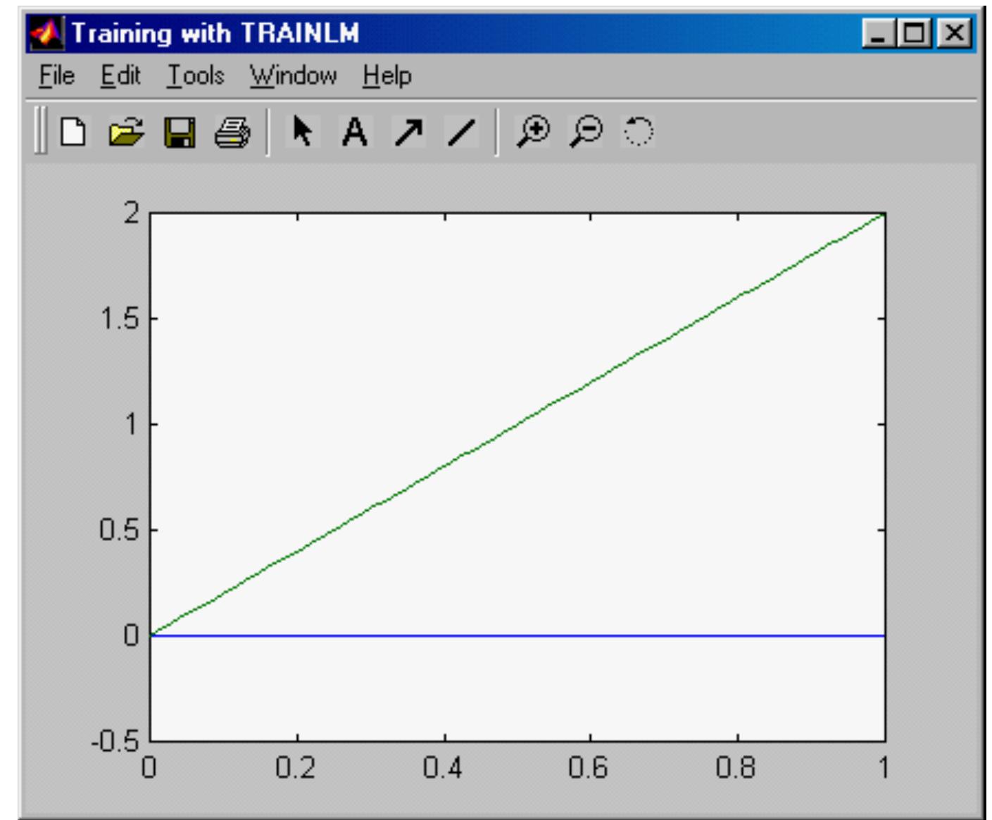
PROBLEM 6. Fit a multilayer perceptron network on y = 2x.

Prune the network size with NNSYSID.

x=0:0 The topology function TFCN can be HEXTOP, GRIDTOP, or RANDTOP. The distance function can be LINKDIST, DIST, or MANDIST.

a,P,a-T) xlabel('time in secs');ylabel('Network output and error'); title('First order bessel function'); grid

Since the error is fairly significant, let's reduce it by doubling the nodes in the first hidden layer to 20 and decreasing the error tolerance to 10 -4 . After plotting this results in the following figure.

The result is considerably better, although it would still require improvement. This is left as further exercise to the reader. Apply vector notation

First construct a Simulink model of Van der Pol system. It is shown below. Call it vdpol.

Recall that initial conditions can be defined by opening the integrators. For example the initial condition x 1 (0) = 2 is given by opening the corresponding integrator.

Use initial condition x 1 (0) = 1, x 2 (0) = 1. net.trainParam.show = 50;net.trainParam.lr = 0.05;net.trainParam.epochs = 1000;net.trainParam.goal = 1e-3; %Train network net1 = train(net, P, T);gi=input(' Strike any key...'); TRAINLM, Epoch 0/300, MSE 4.97149/0.001, Gradient 340.158/1e-010 TRAINLM, Epoch 50/300, MSE 0.0292219/0.001, Gradient 0.592274/1e-010 TRAINLM, Epoch 100/300, MSE 0.0220738/0.001, Gradient 0.777432/1e-010 TRAINLM, Epoch 150/300, MSE 0.0216339/0.001, Gradient 1.17908/1e-010 TRAINLM, Epoch 200/300, MSE 0.0215625/0.001, Gradient 0.644787/1e-010 TRAINLM, Epoch 250/300, MSE 0.0215245/0.001, Gradient 0.422469 The result is not very good, so let's try to improve it.

Using 20 nodes in the hidden layer gives a much better result. The result is displayed in the following figure.

The result is comparable with the previous one.

Try also other initial conditions. If x 1 (0) = 2, and another net is fitted, with exactly the same procedure, the result is shown in the following figure.

It is apparent that for a new initial condition, a new neural network is needed to approximate the result. This is neither very economic nor practical procedure. In example 6, a more general procedure is presented, which is often called hybrid model. The right-hand side of the state equation, or part of it, is approximated with a neural network and the resulting, approximating state-space model is solved. EXAMPLE 5. Solve linear differential equation in the interval [0, 10].

is a unit step. The initial conditions are assumed to be zero. Assume also that the step takes place at t = 0 s. (In Simulink the default value is 1 s.). The output x(t) is your data. Fit multilayer perceptron and radial basis function networks on the data and compare the result with the original data. Add noise to the data and do the fit. Does neural network filter data? SOLUTION: Set up the SIMULINK configuration for the system. Call it linearsec. In simulation use fixed step, because then the number of simulation points remains in better control. If variable-step methods are used, automatic step-size control usually generates more data points than you want.

Go to MATLAB Command window. Simulate and plot the result.

for different initial conditions. Function y = f(x) is has been measured and you must first fit a neural network on the data. Use both backpropagation and radial basis function networks. The data is generated using y=f(x)=sin(x).

-5.0000 0.9589 -4.6000 0.9937 -4.2000 0.8716 -3.8000 0.6119 -3.4000 0.2555 -3.0000 -0.1411 -2.6000 -0.5155 -2.2000 -0.8085 -1.8000 -0.9738 -1.4000 -0.9854 -1.0000 -0.8415 -0.6000 -0.5646 -0.2000 -0.1987 0.2000 0.1987 Instead of typing the data generate it with the following SIMULINK model shown below.

When you use workspace blocks, choose Matrix Save format. Open To workspace block and choose Matrix in the Menu and click OK. In this way the data is available in Command side.

The simulation parameters are chosen from simulation menu given below, fixed-step method, step size = 0.2. Observe also the start and stop times. SIMULINK can be used to generate handily data. This could also be done on the command side. Think of how to do it. %Define parameters net.trainParam.show = 50;net.trainParam.lr = 0.05;net.trainParam.epochs = 500;%Train network net1 = train(net,P,T); TRAINLM, Epoch 0/500, MSE 15.6185/0.001, Gradient 628.19/1e-010 TRAINLM, Epoch 3/500, MSE 0.000352872/0.001, Gradient 0.0423767/1e-010 TRAINLM, Performance goal met.

The figure below shows convergence. The error goal is reached.

The result of the approximation by multilayer perceptron network is shown below together with the error.

a=sim(net1,P); plot (P,a,P,a-T,P,T)

xlabel('Input x');ylabel('Output y');title('Nonlinear function f(x)')

There is still some error, but let us proceed. Now we are ready to tackle the problem of solving the hybrid problem in SIMULINK. In order to move from the command side to SIMULINK use command gensim. This will transfer the information about the neural network to SIMULINK and at the same time it automatically generates a SIMULINK file with the neural network block. The second argument is used to define sampling time. For continuous sampling the value is -1.

gensim(net1,-1)

If you open the Neural Network block, you can see more details.

Open Layer 1. You'll see the usual block diagram representation of Neural Network Toolbox. In our examples, Delays block is unity map, i.e., no delays are in use.

Open also the weight block. The figure that you see is shown below. The number of nodes has been reduced to 5, so that the figure fits on the page. In the example we have 20.

The result is plotted below. plot (tout,yout,tout,yhybrid) title ('Nonlinear system'); xlabel('Time in secs'); ylabel('Output of the real system and the hybrid system'); grid;

Careful study shows that some error remains. Further improvement can be obtained either by adding the network size or e.g. tightening the error tolerance bound.

If the data is noise corrupted the procedure is the same, except that it is recommended that data preprocessing is performed. The data is shown below.

The following SIMULINK model shown below is configured to simulate noise-corrupted data.

The result of the approximation by multilayer perceptron network is shown below together with the error.

As can be seen in the figure, there is still error, but since the given data is noisy, we are reasonably happy with the fit. Preprocessing of data, using e.g. filtering, should be carried out before neural network fitting. Now we are ready to tackle the problem of solving the hybrid problem in SIMULINK. Again use command gensim.

gensim (net1,-1) To convince ourselves that the block generated with gensim really approximates the given data, we'll feed in values of x in the range [-6,6]. Use the following SIMULINK configuration for comparison. What has not been studied is how well they suit for approximating hard nonlinearities.

Use SIMULINK to generate input-output data for a. saturation nonlinearity and b. relay.

Determine, which neural network structure would be best for the above. HINT: For deadzone nonlinearity the data generation can be done using sin-function input for appropriate time interval.

PROBLEM 5. A system is described by a first order difference equation

c. Generate data in appropriate range for f(u) and fit a neural network on the data. d. Simulate the system response for exact f(u) and the neural network approximation.

Compare the results. Initial condition could be zero. Input can be assumed to be noise.

Examples

The input vectors defined below are distributed over a 2-dimension input space varying over [0 2] and [0 1]. This data will be used to train a SOM with dimensions [3 5]. Here the SOM is trained and the input vectors are plotted with the map which the SOM's weights has formed. net = train(net,P); plot(P(1,:),P(2,:), '.g','markersize',20) hold on plotsom (net.iw{1,1},net.layers{1}.distances) hold off

Properties

SOMs consist of a single layer with the NEGDIST weight function, NETSUM net input function and the COMPET transfer function.

The layer has a weight from the input, but no bias. The weight is initialized with MIDPOINT.

Adaptation and training are done with ADAPTWB and TRAINWB1, which both update the weight with LEARNSOM.