A Decomposition Theory for Phylogenetic Networks and
Incompatible Characters
Dan Gusfield1,∗ , Vikas Bansal2 , Vineet Bafna2 , and Yun S. Song1,3
1 Department
2 Department
of Computer Science, University of California, Davis
of Computer Science and Engineering, University of California, San Diego
3 Section
of Evolution and Ecology, University of California, Davis
E-mail: gusfield@cs.ucdavis.edu (Dan Gusfield), vibansal@cs.ucsd.edu (Vikas Bansal),
vbafna@cs.ucsd.edu (Vineet Bafna), and yssong@cs.ucdavis.edu (Yun S. Song)
Keywords: Molecular Evolution, Phylogenetic Networks, Perfect Phylogeny, Ancestral Recombination Graph, Recombination, Gene-Conversion, SNP
Running Head: A Decomposition Theory for Phylogenetic Networks
∗ Corresponding
Author:
Dan Gusfield
Department of Computer Science
University of California, Davis
2063 Kemper Hall
Davis, CA 95616
U.S.A.
Tel: +1 530 752 7131
Fax: +1 530 752 4767
gusfield@cs.ucdavis.edu
1
Abstract
Phylogenetic networks are models of evolution that go beyond trees, incorporating non-tree-like
biological events such as recombination (or more generally reticulation), which occur either in a
single species (meiotic recombination) or between species (reticulation due to lateral gene transfer
and hybrid speciation). The central algorithmic problems are to reconstruct a plausible history of
mutations and non-tree-like events, or to determine the minimum number of such events needed
to derive a given set of binary sequences, allowing one mutation per site. Meiotic recombination,
reticulation and recurrent mutation can cause conflict or incompatibility between pairs of sites (or
characters) of the input. Previously, we used “conflict graphs” and “incompatibility graphs” to
compute lower bounds on the minimum number of recombination nodes needed, and to efficiently
solve constrained cases of the minimization problem. Those results exposed the structural and
algorithmic importance of the non-trivial connected components of those two graphs.
In this paper, we more fully develop the structural importance of non-trivial connected components of the incompatibility and conflict graphs, proving a general decomposition theorem (first
presented in Gusfield and Bansal 2005) for phylogenetic networks. The decomposition theorem
depends only on the incompatibilities in the input sequences, and hence applies to phylogenetic
networks of all types, and to any phenomena that causes pairwise incompatibilities. More generally,
the proof of the decomposition theorem exposes a maximal embedded tree structure that exists in
the network when the sequences cannot be derived on a perfect phylogenetic tree. This extends the
theory of perfect phylogeny in a natural and important way. The proof is constructive and leads
to a polynomial-time algorithm to find the unique underlying maximal tree structure. We next examine and fully solve the major open question from Gusfield and Bansal (2005): Is it true that for
every input there must be a fully decomposed phylogenetic network that minimizes the number of
recombination nodes used, over all phylogenetic networks for the input. We previously conjectured
that the answer is yes. In this paper we show that the answer in is no, both for the case that only
single-crossover recombination is allowed, and also for the case that unbounded multiple-crossover
recombination is allowed. The latter case also resolves a conjecture recently stated in Huson and
Klopper (2007) in the context of general reticulation networks. Although the conjecture from Gusfield and Bansal (2005) is disproved in general, we show that the answer to the conjecture is yes in
several natural special cases, and establish necessary combinatorial structure that counterexamples
to the conjecture must posses. We also show that counterexamples to the conjecture are rare (for
the case of single-crossover recombination) in simulated data.
1
Introduction to Phylogenetic Networks and Problems
With the growth of genomic data, much of which does not fit ideal evolutionary-tree models, and
the increasing appreciation of the genomic role of such phenomena as recombination, recurrent
2
and back mutation, horizontal gene transfer, species hybridization, gene conversion, and mobile
genetic elements, there is greater need to understand the algorithmics and combinatorics of phylogenetic networks on which extant sequences were derived (Posada and Crandall, 2001; Morrison,
2005). Meiotic recombination between homologous chromosomes is particularly important in deriving chimeric sequences in a population of individuals of the same species, and understanding
recombination in populations is a fundamental scientific goal. Moreover, recombination in populations is the key element underlying the logic of “association mapping”, an approach that is widely
hoped to be able to efficiently locate genes influencing genetic diseases (Clark, 2003; Zollner and
Pritchard, 2005; Minichiello and Durbin, 2006; Wu, 2007). On a much longer time scale, recombination between different species can occur (due to horizontal gene transfer), resulting in a hybrid
species. This is called “reticulation” in Huson et al. (2005); Huson and Klopper (2007); Moret
et al. (2004). Although meiotic recombination and species reticulation are very different biological events, the evolution of sequences in either biological context can be represented by similar
phylogenetic networks and certain mathematical and algorithmic properties of these networks are
identical or can be translated from one context to the other. In this paper, we study phylogenetic
networks that derive binary sequences. Many of the results apply both to networks representing
meiotic recombination and to networks representing species reticulation, while some of the results
apply only to the case of meiotic recombination.
The assumption that sequences are binary is justified in the case of meiotic recombination by
the infinite sites assumption in population genetics (Hein et al., 2005), which is strongly justified
by the current importance of SNP (single nucleotide polymorphism) data. In SNP data, each
site can generally take on at most two states (alleles) (Chakravarti, 1998; Hinds et al., 2005) in
a population. In the context of reticulation at the species level, the assumption that sequences
are binary comes from that fact that complex evolutionary characters are usually considered to
be binary (being either present or absent) (Felsenstein, 2004). Moreover, as we will detail later,
reticulation problems or often defined by a set of splits (or cuts), each of which must be in some
tree in the network, and these splits are represented by binary sequences.
We begin with a formal definition of a phylogenetic network, primarily in the context of meiotic
recombination; later when appropriate, we discuss how specific definitions and results can be applied
more broadly to general reticulation.
Formal definition of a phylogenetic network: There are four components needed to specify
a phylogenetic network that allows recombination (see Figure 1).
A phylogenetic network N is built on a directed acyclic graph containing exactly one node (the
root) with no incoming edges, a set of internal nodes that have both incoming and outgoing edges,
and exactly n nodes (the leaves) with no outgoing edges. Each node other than the root has either
one or two incoming edges. A node x with two incoming edges is called a recombination node.
3
00000
M
a: 00010
b: 10010
c: 00100
d: 10100
e: 01100
f: 01101
g: 00101
4
00010
3
a: 00010
1
00100
10010
5
2
00101
P
01100
S
b:10010
P
3
c: 00100
S
4
01101
g: 00101
10100
d: 10100
f: 01101
e: 01100
Figure 1: A phylogenetic network that derives the set of sequences M . The two recombinations
shown are single-crossover recombinations, and the crossover point is written above the recombination node. In general the recombinant sequence exiting a recombination node may be on a path
that reaches another recombination node, rather than going directly to a leaf. Also, in general, not
every sequence labeling a node also labels a leaf.
Each integer (site) from 1 to m is assigned to exactly one edge in N , but for simplicity of
exposition, none are assigned to any edge entering a recombination node. There may be additional
edges that are assigned no integers. We use the terms “column” and “site” interchangeably.
Each node in N is labeled by an m-length binary sequence, starting with the root node which
is labeled with some sequence R, called the “root” or the “ancestral” sequence. Since N is acyclic,
the nodes in N can be topologically sorted into a list, where every node occurs in the list only
after its parent(s). Using that list, we can constructively label the non-root nodes with well-defined
sequences in order of their appearance in the list, as follows:
a) For a non-recombination node v, let e be the single edge coming into v. The sequence labeling
v is obtained from the sequence labeling v’s parent by changing the state (from 0 to 1, or from
1 to 0) of site i, for every integer i assigned to edge e. This corresponds to a mutation at site i
occurring on edge e (i.e., during the interval of time represented by edge e).
b) For a recombination node x, let Z and Z ′ denote the two m-length sequences labeling the
two parent nodes of x. Then the “recombinant sequence” X labeling node x can be any m-length
sequence provided that at every site i in X, the state (0 or 1) is equal to the state at site i in (at
least) one of the sequences Z or Z ′ .
The creation of sequence X from Z and Z ′ at a recombination node is called a “recombination
event”. To fully specify the recombination event, we must specify for every site i in X whether the
binary state in X “comes from” Z or Z ′ . This specification is forced when the states in Z and Z ′ at
site i are different. When they are the same, a choice must be specified. For a given recombination
4
event, we say that a crossover or breakpoint occurs at site i if the states in X at sites i − 1 and i
come from different parents. It is easy to determine the minimum number of crossovers needed to
create X by a recombination of specific sequences Z and Z ′ .
The sequences labeling the leaves of N are the extant sequences, i.e., the sequences that can
be observed. We say that an phylogenetic network N derives (or explains) a set of n sequences M
(each of length m) if and only if each sequence in M labels one of the leaves of N . Without loss of
generality, we assume that there is no site i where all the sequences have the same state at site i.
We also assume throughout that M does not contain any duplicate rows.
With these definitions, the classic “perfect phylogeny” tree (Gusfield, 1991) is a phylogenetic
network with no recombination nodes. That is, each site mutates exactly once in the evolutionary
history, and there is no recombination between sequences.
Note that in the definition above, there is no bound on the number of crossovers that are allowed
at a recombination event (other than the number of sites minus one). Thus, this form of recombination is called “unbounded multiple-crossover” recombination. The main decomposition theorem
in this paper applies even when unbounded multiple-crossovers are allowed, and as we will show,
multiple crossovers allows us to model a wide variety of biological phenomena. However, in meiotic
recombination the number of crossovers is typically small, and the algorithmic/mathematical literature motivated by meiotic recombination has mostly assumed that only one crossover is allowed
in a recombination event. This is called “single-crossover recombination”, and when it occurs the
recombinant sequence X is formed from a prefix of one of its parent sequences (Z or Z ′ ) followed
by a suffix of the other parent sequence. That is the definition of recombination used in our early
publications on phylogenetic networks, for example Gusfield et al. (2004a,b). A few papers have
studied two-crossover recombination events motivated by “homologous gene-conversion” in Song
et al. (2006). For brevity, we will use the phrase “multiple-crossover recombination” to mean “unbounded multiple-crossover recombination”. Some mathematical and algorithmic results depend on
whether each recombination event is restricted to a single-crossover, or whether multiple-crossovers
are allowed, and we will be very careful about that distinction.
What we have defined here as a phylogenetic network with single-crossover recombination is
the digraph part of the stochastic process called an “ancestral recombination graph (ARG)” in the
population genetics literature (Griffiths and Marjoram, 1996). (See also Norborg and Tavare 2002
or Hein et al. 2005 for an introduction to ARGs).
Rooted and Root-Unknown problems: Problems of reconstructing phylogenetic networks,
given an input set of binary sequences M , can be addressed either in the rooted case, or the rootunknown case. In the rooted phylogenetic network problem, a required root or ancestral sequence
R for the network is specified in advance. In the root-unknown phylogenetic network problem, no
ancestral sequence is specified in advance, and the algorithm must select an ancestral sequence at
5
the root.
The algorithmic problem of reconstructing a history of recombination events (with mutations),
or determining the minimum number of recombination nodes needed in a phylogenetic network
(for both rooted and unrooted problems), has been studied in a number of papers (Gusfield et al.,
2007; Hein, 1990, 1993; Song and Hein, 2003, 2004; Wang et al., 2001; Myers and Griffiths, 2003;
Hudson and Kaplan, 1985; Kececioglu and Gusfield, 1998; Gusfield, 2005a; Gusfield et al., 2004b,a;
Nakhleh et al., 2003, 2004; Moret et al., 2004; Bafna and Bansal, 2004, 2006a; Song et al., 2005;
Lyngso et al., 2005; Song et al., 2006; Myers, 2003).
2
A Fundamental Decomposition Theory
In this section we define and state the main result of this paper, the decomposition theorem. It
will be proved in the next section. We believe the decomposition theorem and insights obtained
from its proof are fundamental and extend the theory of perfect phylogeny from trees to general
phylogenetic networks. We now begin the needed definitions and facts that lead to the statement
of the main result.
2.1
Recombination Cycles and Blobs
In a phylogenetic network N , let w be a node that has two paths out of it that meet at a recombination node x. Those two paths together define a “recombination cycle” Q. Node w is called
the “coalescent node” of Q, and x is the recombination node of Q. In Figure 1, the nodes labeled
00000 and 00100 are coalescent nodes of two different recombination cycles.
A recombination cycle that is node-disjoint from any other recombination cycle has been defined
as a “gall” (Gusfield et al., 2004b; Gusfield, 2005a; Song, 2006b). If a recombination cycle is edgedisjoint from any other recombination cycle in the network, then the network can be modified so
that the cycle is node-disjoint from any other cycle. The modification requires adding one new
edge and one new node, with the same sequence labeling both ends of the new edge. Repeating
this as needed, we can assume that if a recombination cycle does not share an edge with any other
recombination cycle, then it also does not share a node with any other recombination cycle. In
contrast, consider a recombination cycle that shares at least one edge with some other recombination
cycle. We can add another cycle to those two if the new cycle shares an edge with one of the two
cycles. Continuing in this way, adding more cycles, we ultimately get a well-defined maximal set
of recombination cycles in N that form a single connected subgraph of N , and each cycle shares
at least one edge with some other cycle in the set. We call such a maximal set of recombination
cycles a “blob”.
Clearly, because of maximality, the blobs in a phylogenetic network N are well-defined, i.e.,
each blob can be found as above, starting from any recombination cycle in the blob. Moreover, as
6
above, we assume that no blob shares a node with any other blob. Therefore, if we contract each
blob in a network N to a single point, the resulting network is a directed tree T ′ . This follows
because if the resulting graph had a cycle (in the underlying undirected graph) that cycle would
correspond to a recombination cycle in N which should have been contracted. We call T ′ a “tree
of blobs” or a “blobbed tree”. So every phylogenetic network N can be viewed as a blobbed tree.
The edges in T ′ are called “tree edges” of N .
2.2
Incompatibility and Perfect Phylogeny
The main tools that we used in Gusfield et al. (2004b, 2007); Gusfield (2005a); Bafna and Bansal
(2004); Song (2006b) and other papers were two graphs representing “incompatibilities” and “conflicts” between sites. We introduce these graphs here.
Given a set of binary sequences M , two columns i and j in M are said to be incompatible if
and only if there are four rows in M where columns i and j contain all four of the ordered pairs
0,1; 1,0; 1,1; and 0,0. For example, in Figure 1 columns 1 and 3 of M are incompatible because
of rows a, b, c, d. The test for the existence of all four pairs is called the “four-gamete test” in
the population genetics literature. A site that is not involved in any incompatibility is called a
“compatible site”.
Given a sequence S, two columns i and j in M are said to conflict (relative to S) if and only
if columns i and j contain all three of the above four pairs that differ from the i, j pair in S. It is
easy to see that two columns conflict relative to S if and only if they are incompatible in M + S,
the set resulting from adding sequence S to M .
The classic Perfect Phylogeny Theorem (in the terminology of this paper) is: There is a rooted
phylogenetic network N without recombination cycles that derives a set of binary sequences M , if
and only if there is no incompatible pair of columns in M . Network N is a directed tree T , with
the root labeled by a sequence that need not be in M . Moreover, the undirected tree created by
ignoring the directions of the edges of T is invariant over all perfect phylogenies for M . Similarly,
there is a unique phylogenetic network that derives M , with ancestral sequence S and without
recombination cycles (and hence is a directed tree), if and only if there is no pair of columns that
conflict relative to S. For one exposition of these classic results, see Gusfield (1997). For different
expositions, see Theorem 3.1.4 in Semple and Steel (2003) or the Pairwise Compatibility Theorem
in Felsenstein (2004).
Incompatibility and Conflict Graphs: We define the “incompatibility graph” G(M ) for M
as a graph containing one node for each column (site) in M , and an edge connecting two nodes i
and j if and only if columns i and j are incompatible. Similarly, given a sequence S, we define the
“conflict graph” GS (M ) for M (relative to S) as a graph containing one node for each column in
M , and an edge connecting two nodes i and j if and only if columns i and j conflict relative to S.
7
00000
4
00010
3
a: 00010
1
00100
10010
P
b:10010
M
a: 00010
b: 10010
c: 00100
d: 10100 Incompatibility Graph
e: 01100 for M.
f: 01101
g: 00101
1 2 3 4 5
S
00100
c: 00100
3
5
2
10100
00101
01100
P
d: 10100
e: 01100
S
4
g:00101
01101
f: 01101
Figure 2: The incompatibility graph G(M ) for the sequences M from Figure 1, and a fullydecomposed phylogenetic network that derives M . This network is also a galled-tree for M .
It is easy to see that GS (M ) = G(M ) if S ∈ M , and so GS (M ) = G(M + S). Figure 2 shows the
incompatibility graph G(M ) for M from Figure 1.
A “connected component” (or “component” for short), C, of a graph is a maximal subgraph
such that for any pair of nodes in C there is at least one path between those nodes in the subgraph.
A “trivial” component has only one node, and no edges. The incompatibility graph in Figure 2 has
two components. Previously (Gusfield et al., 2004b; Gusfield, 2005a; Gusfield et al., 2007, 2004a;
Bafna and Bansal, 2004), the non-trivial connected components of the conflict and incompatibility
graphs were shown to be very informative, used both to derive efficient algorithms and to expose
combinatorial structure in phylogenetic networks. The structural importance of the non-trivial
connected components is further developed in the main result, presented next.
2.3
The Decomposition Theorem
Theorem 1. Let G(M ) be the incompatibility graph for M . Then, there is a phylogenetic network
N that derives M where every blob in N contains all and only the sites of a single non-trivial
connected component of G(M ), and every compatible site is on a tree edge of N . The result holds no
matter what constraints, if any, are placed on the number of crossovers allowed at a recombination
node.
Stated another way, for any input M , there is a blobbed-tree that derives M , where the blobs
are in one-one correspondence with the non-trivial connected components of G(M ), and if bC is
the blob corresponding to component C, then bC contains all and only the sites in C. We call
a network “fully-decomposed” if it has the structure specified in Theorem 1. Figure 2 shows a
fully-decomposed network for the sequences M from Figure 1.
Theorem 1 is an extension of the stronger theorem proved in Gusfield et al. (2004b) about
8
galled-trees. In the case of galled-trees, every reduced galled-tree for M must be fully-decomposed.
A galled-tree is “reduced” if every recombination cycle contains some incompatible sites. When
there is a galled-tree for M , there is a reduced galled-tree for M , and it can be found in polynomial
time (Gusfield et al., 2004b; Gusfield, 2005a). This strong decomposition property of galled-trees
was one of the main motivations for investigating decomposition in general phylogenetic networks
and the general role of connected components of G(M ) in decomposition.
It is easy to prove (Gusfield et al., 2004b) a statement converse to Theorem 1: In any phylogenetic network N that derives M , all sites from the same non-trivial connected component of
G(M ) must appear on the same blob in N , and this does not depend on the number of crossovers
used at recombination node. That is, it is not possible to split up the sites from a connected
component of G(M ) into two or more blobs in N . Therefore the network that is guaranteed by
the Decomposition Theorem is as highly decomposed into distinct blobs as possible, justifying the
term “fully-decomposed”.
There is an analogous theorem to Theorem 1 in the case that the ancestral sequence S is known
in advance. In that case, there is a phylogenetic network N that derives M , with ancestral sequence
S, where the blobs in N are in one-one correspondence with the non-trivial connected components
of GS (M ), and any non-conflicting site is on a tree edge of N ; again, no further decomposition is
possible. This follows from Theorem 1, and the fact that two sites conflict relative to S if and only
if they are incompatible in M + S.
We will prove the Decomposition Theorem in the next section and show that the tree parts of
any fully-decomposed phylogenetic network are invariant.
3
Proof of The Decomposition Theorem
In this section we prove Theorem 1.
3.1
The structure of M
Let C and C ′ be two distinct connected components in the incompatibility graph G(M ), and assume
first that C is non-trivial. C ′ might be a trivial connected component, i.e., consist of only a single
node. For any pair of sites i ∈ C, i′ ∈ C ′ let (X, X) and (Y, Y ) be the respective bipartitions (of the
rows of M ), associated with sites i and i′ . The two bipartitions cannot be identical, for otherwise
sites i and i′ would have exactly the same incompatibilities and so be in the same connected
component. Each of the four subsets X, X, Y, Y is called a “class” of the bipartition it is part of.
Sites i and i′ are not incompatible, so one class of the i bipartition must strictly contain one class
of the i′ bipartition, and the other class of the i′ bipartition must strictly contain the other class
of the i bipartition. Without loss of generality, suppose X ⊃ Y and Y ⊃ X. We say that X is the
“dominant” class of i, and X is the “dominated” class, with respect to the pair i, i′ . Similarly, Y is
9
the dominant class of i′ , and Y is the dominated class, with respect to the pair i, i′ . For example,
in Figure 2, C = {1, 3, 4} and C ′ = {2, 5}, and with respect to the pair 1, 2, the set {a, c, e, f, g} is
the dominant class, and {b, d} is the dominated class.
Now consider the case that sites i and i′ are the sites of two trivial components C and C ′ . If i
and i′ are not identical, then one class of i, say X, must strictly contain a class, say Y , of i′ , and
so X and Y are again the well-defined dominant classes of i and i′ , with respect to i, i′ . If sites i
and i′ are identical, and say X = Y , then we arbitrarily choose the pair X, Y or X, Y as the two
dominant classes of i and i′ respectively.
Lemma 1. Let i, i′ , C, C ′ , X, and Y be as above. Let j ′ be any site in C ′ , and let (Z, Z) be the
bipartition associated with j ′ . Then, the dominant class of i with respect to the pair i, j ′ is the
dominant class of i with respect to the pair i, i′ .
Proof. The Lemma is vacuously true if C ′ is a trivial connected component, so assume C ′ is nontrivial. We need to show that either X ⊃ Z or X ⊃ Z. Consider a site k′ ∈ C ′ that is incompatible
with i′ . Such a site k′ must exist since C ′ is connected. Let (W, W ) be the bipartition defined by
site k′ . If X is not dominant with respect to i, k′ , then X is dominant with respect to i, k′ , and so
either X ⊃ W or X ⊃ W . Suppose that X ⊃ W , so W ⊃ X. But then W ⊃ Y since X ⊃ Y , and
so Y ∩ W = ∅, and i and k′ can’t be incompatible, which is a contradiction. Similarly, if X ⊃ W ,
then W ⊃ X, so W ⊃ Y , and W ∩ Y = ∅, a contradiction. So the dominant class, X, with respect
to i, i′ is the dominant class with respect to i, k′ , where k′ is any site that is incompatible with
i′ . The Lemma now follows by transitivity, because C ′ is a connected component, so from i′ it is
possible to reach any j ′ ∈ C ′ by a series of incompatibility relations.
Lemma 1 establishes that for any i ∈ C, one class of i is dominant with respect to all sites in
C ′ , and symmetrically, for any i′ ∈ C ′ one class of i′ is dominant with respect to all sites in C. So,
with respect to the (C, C ′ ) pair of connected components, each site in C ∪ C ′ has a well-defined
dominant class, and a well-defined dominated class.
Now return focus to the sequences in M and the sites in C and C ′ . For a site i ∈ C, the
bipartition (X, X) is encoded with 0’s and 1’s, where all the rows in X have one character at site
i and all the rows in X have the other character at site i. So, with respect to the (C, C ′ ) pair of
connected components, and a specific set of sequences M , each site in C has a well-defined dominant
character (either 0 or 1). For example, in Figure 3, the dominant character is 0 in all sites except
3, where the dominant character is 1.
Let D[C, C ′ ] be the union of the rows in the dominated classes of C, with respect to (C, C ′ ).
Similarly, let D[C ′ , C] be union of the rows in the dominated classes of C ′ , with respect to (C, C ′ ).
For example, D[C, C ′ ] is {a, b, d} and D[C ′ , C] is {e, f, g} in Figure 3.
Let M (C) and M (C ′ ) be the sequences in M , restricted to the sites in C and C ′ respectively.
Then Lemma 1 implies
10
1
3
4
2
5
a
0
0
1
0
0
b
1
0
1
0
0
d
1
1
0
0
0
c
0
1
0
0
0
e
0
1
0
1
0
f
0
1
0
1
1
g
0
1
0
0
1
Figure 3: The sites in the two connected components from Figure 2. We denote the component
with sites {1, 3, 4} as C, and the component with sites {2, 5} as C ′ . The dominant sequence for C
is 010, and the dominant sequence for C ′ is 00. The rows in D[C, C ′ ] are {a, b, d}, and the rows
in D[C ′ , C] are {e, f, g}. The rows and columns have been permuted from their natural order to
collect together the sites in the two components, and the rows in D[C, C ′ ] and D[C ′ , C]. Note that
row c is in neither D[C, C ′ ] nor D[C ′ , C], since row c has the dominant sequence in both its C and
C ′ sides.
Theorem 2. Every row in D[C, C ′ ] has the same sequence in M (C ′ ). In particular, in each row
of D[C, C ′ ], every site i′ ∈ C ′ has the dominant character with respect to (C, C ′ ). Similarly, every
row in D[C ′ , C] has the same sequence in M (C). In particular, in each row of D[C ′ , C], every site
i ∈ C has the dominant character with respect to (C, C ′ ).
Given Theorem 2, we can define the dominant sequence in M (C) with respect to (C, C ′ ) as the
sequence in M (C) where each site has the dominant character with respect to (C, C ′ ). Similarly,
we can define the dominant sequence in M (C ′ ) with respect to (C, C ′ ).
Corollary 1. Let C and C ′ be two connected components of G(M ). There is no row in M which
(w.r.t. (C, C ′ )) contains both a non-dominant sequence in M (C) and a non-dominant sequence in
M (C ′ ).
Figure 3 illustrates Lemma 1, Theorem 2 and Corollary 1. Note that a row can have both the
dominant sequence in M (C) and the dominant sequence in M (C ′ ). Row c in Figure 3 is an example
of this. Corollary 1 is a more refined version, and with a simpler proof, of a result (Theorem 3)
first proved in Bafna and Bansal (2004).
We develop here an observation that will be needed in Section 5.2. Consider two sites i ∈ C
and i′ ∈ C ′ , where C and C ′ are two distinct non-trivial connected components of G(M ). By
assumption, every column contains both a 0 and a 1. Also, any two columns in different non-trivial
components must not be identical (or exact compliments of each other) or else they would both be
11
incompatible with the same sites in C and C ′ , and hence would be in the same component. So,
there must be at least three distinct pairs of binary characters in columns i, i′ . But, since i and
i′ are not incompatible, there cannot be four distinct pairs binary characters in those columns, so
there must be exactly three distinct pairs of binary characters in columns i, i′ . Hence, if we add
new sequences to M , creating the set M , and i and i′ are not incompatible in M , then any pair
of binary characters in M in columns i, i′ , must already have been a pair of binary characters in
columns i, i′ in M . Therefore, with respect to (C, C ′ ), the dominant characters in C and C ′ created
from M are the same as the dominant characters of C and C ′ created from M . Extending this
observation to all sites in C and C ′ we have:
Lemma 2. Suppose C and C ′ are non-trivial components of G(M ). If we add new sequences to
M which do not create any incompatibilities between sites in different components of G(M ), then
with respect to (C, C ′ ), the dominant sequences of C and C ′ remain unchanged.
3.2
The super-characters of M and the new matrix B
Lemma 1, Theorem 2 and Corollary 1 establish a structure that exists in M , imposed by the
partition of the columns of M by the connected components of G(M ). We begin now to exploit
that structure to prove the Decomposition Theorem. We define a new set of binary sequences B
created from M and G(M ), and represent the set B as a matrix, as follows. Let C be a connected
component of G(M ) and let M (C) be the sequences in M restricted to the sites in C. We call each
distinct sequence in M (C) a super-character of M (associated with C). For every C, we create one
column, s in B for each super-character S of M , where S ∈ M (C). We say that s originates from
S and from C. Each such column in B encodes a bipartition of the rows of M where one side of
the bipartition contains all the sequences in M that contain subsequence S in M (C), and the other
side of the bipartition contains the remaining sequences. More specifically, and without loss of
generality, in the new column we assign value 1 to each sequence in M which contains subsequence
S in M (C), and assign value 0 to each sequence that does not. The new column defines a binary
character derived from M and G(M ). Note that if C is a trivial connected-component, so it only
contains one site, then B will have two columns derived from that one site, but those columns define
the same bipartition. That will cause no problems, and one column can be removed for simplicity.
As an example, Figure 4 shows the matrix B that is derived from M and G(M ) from Figure 2.
We will use the characters of B to build a tree in order to prove Theorem 1.
Lemma 3. No pair of characters of B are incompatible.
Proof. Let p and q be distinct characters in B. If p and q originate from the same connected
component C in G(M ), then by construction, no row can have a 1 in both columns p and q and
therefore, characters p and q are not incompatible.
12
1
2
3
4
5
6
7
8
a
1
0
0
0
1
0
0
0
b
0
1
0
0
1
0
0
0
c
0
0
1
0
1
0
0
0
d
0
0
0
1
1
0
0
0
e
0
0
1
0
0
1
0
0
f
0
0
1
0
0
0
1
0
g
0
0
1
0
0
0
0
1
Figure 4: Matrix B derived from M and G(M ) from Figure 2. The super-characters of M associated
with C are 001, 101, 010, 110, and the super-characters of M associated with C ′ are 00, 10, 11, 01.
The columns (characters) of B are ordered to correspond to those ordered lists of super-characters
of M .
Now suppose p and q originate from two different connected components C and C ′ in G(M ).
If p and q both originate from the non-dominant sequences (w.r.t. (C, C ′ )) of C and C ′ , then
Corollary 1 guarantees that there is no row with 1, 1 in columns p and q, and so p and q cannot be
incompatible. Symmetrically, if p and q both originate from dominant sequences (w.r.t. (C, C ′ ))
of C and C ′ , then there is no row with 0, 0 in columns p and q. If p originates from the dominant
sequence (w.r.t. C, C ′ ) of C and q originates from a non-dominant sequence (w.r.t. C, C ′ ) of C ′ ,
then there can be no 0, 1 in columns p and q. The remaining case is symmetric.
Applying the Perfect Phylogeny Theorem, Lemma 3 establishes that there is a perfect phylogeny
T where each character of B labels one edge in T , and each edge is labeled by one or more characters
of B. Since each character of B originates from a super-character of M , it will sometimes also be
useful to think of edge labels as being super-characters of M .
3.3
Inflating T
The next step is to inflate nodes of T to blobs in order to create a fully-decomposed phylogenetic
network N for M , proving Theorem 1.
The removal of any edge e in T creates two connected subtrees, and we define a “split of edge
e” as the bipartition of the leaves resulting from the removal of edge e from T . From the facts
that all columns in B are distinct, and that every edge in T is labeled, it follows that all the splits
defined by the edges in T are distinct. If e is labeled by character c of B, we define the “1-side”
of e as the subtree of T − e that contains the leaves for rows in B that have value 1 for character
c. The other side is called the “0-side” of the split. When no root sequence has been specified in
advance, the root could be on either side of the split.
13
Lemma 4. Let C be an arbitrary component of G(M ). In T , there is a node vC such that all the
edges labeled by characters of B that originate from connected component C, are incident with vC .
That is, these edges form a star around a single central node vC . Further, vC is on the 0-side of
each split defined by an edge labeled by a character of B that originates from C.
Note however, that Lemma 4 does not assert that vC is only incident with edges labeled by
characters that originate from C.
Proof. First, the Lemma is trivially true if C is a trivial component since only one character
originates from C and it labels only one edge. For any non-trivial connected component C, the
submatrix M (C) contains at least four distinct sequences since there are must be at least one
(incompatible) pair of sites in C where all four binary pairs appear in M (C). Therefore, there are
at least four characters in B that originate from C. Let B(C) denote the columns of B restricted
to the characters that originate from C.
Consider a non-trivial connected component C and any three of characters of B that originate
from C, and let e1 , e2 , e3 be the three edges in T labeled with those characters. Note that every
row in B has value 1 in exactly one column of B(C), so every leaf of T is on the 1-side of exactly
one edge labeled by a character from C. Hence, no leaf in T can be on the 1-side of two of the
edges e1 , e2 , e3 .
Now, consider the undirected tree created by ignoring the directions of the edges in T , but we
will still refer to this undirected tree as T . If e1 and e2 are incident with each other, sharing a node
v, then there must be another edge incident with node v, and hence there must be a leaf lv that
is reachable from v without going through e1 or e2 . If this were not true, then e1 and e2 would
define the same splits in T , which is not possible. If e1 and e2 are not incident with each other,
then there is a unique shortest path P from an endpoint of e1 to an endpoint of e2 . Clearly, path
P does not contain edge e1 or e2 . There must be a node v on P and a leaf lv that is reachable from
v via a path that does not go through e1 or e2 . If this were not true, then again there would be
two adjacent edges that define the same splits in T .
Now we claim that node lv must be on the 0-side of both e1 and e2 . We have already established
that it cannot be on the 1-side of both. However, suppose without loss of generality, that lv is on
the 1-side of e1 and the 0-side of e2 . Then consider the endpoint u of e2 that is on the 1-side of e2 ,
and consider a leaf lu that is reachable from u without going through e2 . Leaf lu would be on the
1-side of both e1 and e2 , which is not possible. Hence the 1-sides of both e1 and e2 point “away”
from each other. It also follows that path P cannot go through edge e3 . If it did, then some leaf
on the 1-side of e3 would also be on the 1-side of e1 or e2 .
So edges e1 and e2 are either incident with each other, or there is an edge e which is incident
with e1 on path P , where e is not labeled by a character of B that originates from C. We will
show that such an edge e cannot exist. Every internal edge in T is labeled by some character of
14
B, so suppose e exists and is labeled by a character that originates from a connected component
C ′ . Let v be the common endpoint of e1 and e. As above, there must be a leaf lv that is reachable
from v without going through either edge e or e1 , for otherwise e and e1 define the same split,
which is not possible. Recall that each character of B and each split in T that originates from C or
C ′ , corresponds to a sequence (super-character) in M (C) or M (C ′ ), and with respect to the pair
(C, C ′ ), there is a dominant sequence S in M (C) and a dominant sequence S ′ in M (C ′ ). Let e(S)
be the edge in T labeled by the character that originates from S, and let e(S ′ ) be the edge in T
labeled by the character that originates from S ′ . Now e1 is either e(S) or not, and e is either e(S ′ )
or not, so we have four cases to consider.
Case 1: Suppose e1 is e(S) and e is e(S ′ ). We know that l(v) is on the 0-side of e1 , so it must
be on the 1-side of e by Corollary 1. But then, all leaves on the 0-side of e will be on the 0-side of
both e and e1 , which contradicts Corollary 1. So e cannot exist in this case.
The three other cases are similar and omitted, and the result is that e cannot exist and hence
e1 and e2 are incident with each other. Since e1 and e2 were arbitrary edges labeled by characters
that originated from C, every pair of edges labeled by characters that originate from C must be
incident with each other. But in a tree, that is only possible if all those edges share exactly one
endpoint, and so form a star around a single center. That endpoint is the claimed node vC . We
also established that if there are two distinct edges labeled with characters that originate from C,
then the 1-sides of these edges point away from each other. This holds for any pair of edges labeled
with characters that originate from C, so vC is on the 0-side of every such edge.
3.4
Completion of the proof of the Decomposition Theorem
To finish the proof of the Decomposition Theorem, we first ignore the direction of the edges of
T and ignore which node is its root. Instead, we arbitrarily select a node vr of T to be the root
and direct all the edges in T away from that chosen root. Let S be the label written at node vr
(recall that a perfect phylogeny is a phylogenetic network and so each node is labeled). The label
S will define the ancestral sequence for the phylogenetic network we will construct. Next, we need
to inflate each node vC in T that is the central node of the star associated with the characters
obtained from a non-trivial component C of M (G). Note that vr might also be a central-star node.
We can identify the central-star node vC by the fact that for the non-trivial connected component
C, all of the edges labeled by the characters that originate from C are incident with vC . Each such
edge may also be labeled with characters that originate from another connected component or with
a compatible character. Now, each central-star node vC , other than the root node, has exactly
one edge directed into it; the character on it that originates from C must be the super-character
S(C), defined as sequence S restricted to the sites in C. We call S(C) the “ancestral sequence” of
vC . Similarly, if the root node is associated with the non-trivial component C, then S(C) is the
15
ancestral sequence of vr = vC . Now, any super-character in M that is associated with C can be
derived from S(C) using at most one mutation per site, if an unlimited number of recombination
nodes are allowed. This is true even if only single-crossovers are allowed, or if multiple-crossovers
are permitted1 . So, each central-star node v can be inflated into a blob bv containing one node
labeled by each super-character in M (C), and other nodes if needed. Then for each super-character
associated with C, we connect the node in bv labeled with the character c in B which originates
from that super-character, to the edge incident with vC that is labeled by character c.
After inflating each central-star node in T , the end result is a phylogenetic network N where
each blob contains all and only the sites from one connected component of G(M ). Every compatible
site labels a tree edge of N . The full ancestral sequence for N is specified by the ancestral sequences
defined above, since each site in M is in the ancestral sequence for exactly one central-star node.
This completes the proof of Theorem 1.
Note that the existence and the topology of T depends only on the partition of the nodes
of G(M ) into connected components, and hence does not depend on the biological causes of the
incompatibilities in M . In particular, it does not depend on whether or not multiple-crossovers are
allowed at recombination nodes. However, the networks inside each blob of N do depend on which
biological events (such as single versus multiple-crossover recombination, or recurrent mutation,
etc.) occur there.
3.5
Component-wise optimal decomposition
We can now state a fact that follows easily from Theorem 1 and will be needed in Section 5.2.
Recall that S(C) is the sequence S restricted to the sites in component C. Let RS(C) (M (C)) be
the minimum number of recombination nodes (events) needed to generate the sequences M (C) in
a phylogenetic network with ancestral sequence S(C), when multiple-crossover recombination is
1
allowed. Similarly, let RS(C)
(M (C)) be the minimum number of recombination nodes needed when
only single-crossover recombination is allowed. The proof of Theorem 1, when applied to the set
of sequences M + S, where S is a required ancestral sequence (which might not be in M ), and the
root of T is selected to be the node labeled S, establishes the following:
Theorem 3. For any sequence S, there is a fully-decomposed phylogenetic network for M with anP
cestral sequence S, containing exactly C∈GS (M ) RS(C) (M (C)) recombination nodes when multipleP
1
crossover recombination is allowed, and containing exactly C∈GS (M ) RS(C)
(M (C)) recombination
nodes when only single-crossover recombination is allowed.
1
It is also true that the sequences can be derived from S(C) without recombination if an unlimited number of
recurrent or back mutation events are allowed. Recurrent-mutation occurs when the state of a site mutates from its
ancestral state more than once in an evolutionary history. Back-mutation occurs when the state mutates from the
derived state back to the ancestral state.
16
3.6
Programs
The proof of the existence of T can be converted into an efficient, constructive method2 for finding
T from any input M . The program galledtree.pl, available at
wwwcsif.cs.ucdavis.edu/~gusfield/ takes in a set of sequences M and tries to build a galled-tree for
M using single-crossover recombination. If it succeeds, then it has produced a complete phylogenetic
network for M where each blob is a single cycle, and the cycles are node disjoint. Hence, the program
produces a fully-decomposed phylogenetic network for M . If the program determines that there
is no galled-tree for M , then it outputs the tree T for M . The running time for the program is
O(nm2 + m3 ), but the time used to build T is just O(nm2 ).
3.7
Uniqueness of T
In a network N , we say that a node v in blob b is an external node if there is an edge from v to some
node outside of b. We say a phylogenetic network N is efficient if N does not contain two external
nodes with the same node labels, and for each external node v (in a blob b), there is exactly one
edge from v to a node off of b. Clearly, if N is not efficient, it can be easily modified to become
efficient without increasing the number of recombinations used. Also, if N is fully-decomposed,
then the efficient network derived from it is also fully-decomposed. So for any M , there is a efficient
fully-decomposed phylogenetic network for M .
Theorem 4. If N is any efficient fully-decomposed network for M , and T ′ is created by contracting
each blob of N to a single node, then after the directed edges in T ′ are made undirected, the resulting
tree is necessarily the tree T defined in the proof of Theorem 1.
Proof. Consider a blob bC in N associated with the component C in G(M ); let v be an external node
in bC incident with the edge e = (v, v ′ ), directed from v to a node v ′ off of bC . In the subnetwork
reached from v ′ , all of the sites in C have the same state they have at v ′ . This is because no site
in C mutates outside of bC , and (by induction on the maximum path length from from v ′ to a
recombination node x) at any recombination node x in the subtree, the state of any site in C is
the same at x as it is in both of the parent sequences of x. Now every super-character in M (C) is
a subsequence of some sequence of M , and the super-characters include all the distinct sequences
in M (C), therefore (when restricted to the sites in C) each external node on bC is labeled with a
distinct super-character derived from C, and each super-character derived from C labels exactly
one external node of bC . Consider again node v, labeled with super-character Sv (C) from M (C),
and consider the edge e = (v, v ′ ). If we remove edge e from N , two disconnected subnetworks
2
It may seem that T can be obtained by simply building a perfect phylogeny T using one site from each connected
component of G(M ). However, this is wrong, because the edge structure of T may be very different from that of T .
For example, in the tree T created from sites 1 and 2 in Figure 1, the two edges labeled with those sites are adjacent,
while they are not adjacent in T .
17
are created. In one subnetwork, every leaf label contains Sv (C), and in the other subnetwork, no
leaf label contains Sv (C). The leaf labels are the sequences of M , and so the removal of e from
N creates a bi-partition of the sequences in M . Clearly then, edge e defines exactly the same
bi-partition of the sequences in M that is defined by the split K in T created by removing from
T the edge labeled by the character that derives from super-character Sv (C). Now edge e is also
contained in tree T ′ , and its removal from T ′ creates the same bi-partition that it does in N , and
so the removal of e from T ′ creates the split K. Therefore, the splits in T ′ are exactly the same as
the splits in T . By Theorem 3.1.4 (the Splits Equivalence Theorem) in Semple and Steel (2003),
the splits of an undirected tree uniquely define the tree, and so the undirected trees, T ′ and T are
identical.
In other words, T is the invariant underlying structure of any efficient fully-decomposed phylogenetic network for M , and this is true regardless of the biological causes of the incompatibilities
in M . We will need this fact in Section 5.1.
3.8
Alternate Proofs of Theorem 1
Theorem 1 was first stated and proved in Gusfield and Bansal (2005). It has been pointed out
(Steel, 2005) that Theorem 1 can also be proven by using Buneman graphs (Semple and Steel,
2003), and the details of this approach have been verified (Wu, 2005). However, the proof here
is more direct and establishes a polynomial time algorithm to construct T . In contrast, it takes
exponential time in worst case to build a Buneman graph from M , and so that is not an efficient
constructive approach to building T from M . Another direct proof of Theorem 1 that is shorter than
the one presented here, but does not establish or emphasize the role of super-characters, appears
in a 2006 preprint by Bafna and Bansal (2006b). Subsequent to the development of Theorem 1, a
related decomposition theorem was developed (Huson et al., 2005) where the input to the problem
is not a set of sequences, but a set of trees that must be subtrees in a constructed phylogenetic
network.
4
4.1
Broader Applications
Alternate causes of incompatibility
In the proof of the Decomposition Theorem, there was no mention of recombination until close to the
end of the proof, when discussing the inflation of the central-star nodes. Therefore, all the results
proven to that point hold for any incompatible characters of M , independent of the biological
cause of the incompatibilities. Also, the proof of uniqueness did not depend on recombination.
Hence, the existence, structure and uniqueness of T holds for any M and any biological cause
of incompatible characters. In this way, we have established that the super-characters of M ,
18
defined by the connected components of G(M ), generalize standard evolutionary characters (used
in phylogenetic trees), and play a role in the theory of phylogenetic networks that tree characters
play in the theory of phylogenetic trees. Moreover, if the biological operations that caused the
incompatibilities in M allow any set of sequences M (C) to be derived from an arbitrary ancestral
sequence, then the Decomposition Theorem holds in that biological context.
Another way to see the generality of the results proven here is to note that multiple crossover
recombination can be considered as a mathematical operation on binary sequences rather than a
biological event, and can be used to model biological events that don’t explicitly involve recombination. For example, an occurrence of back-mutation or recurrent-mutation of a site i in a sequence S
can be modeled as a two-crossover recombination between S and some appropriate sequence, in the
intervals i − 1, i and i, i + 1. Modeling back and recurrent mutations in this way explicitly creates
recombination cycles and blobs, and shows explicitly how Theorem 1 applies when back-mutation
and/or recurrent mutation cause incompatibilities. Generally, when back or recurrent mutation
is the cause of incompatibility, we seek an evolutionary tree that derives a given set of sequences
using as few back or recurrent mutations as possible. Such a tree is called a “maximum parsimony
tree” and it is a solution to the maximum parsimony problem (Felsenstein, 2004; Semple and Steel,
2003).
4.2
What is the “most tree-like” phylogenetic network?
When a set of sequences M fails the four-gametes test and hence cannot be generated on a perfect
phylogeny, one would still like to derive the sequences on a phylogenetic network that is the “most
tree-like”. There is no accepted definition of “treeness”, and under many natural definitions, the
problem of finding the most tree-like network would likely be computationally difficult. In this
section, we introduce a measure of treeness and relate it to Theorem 1.
Recall that it is assumed that in network N no two blobs share a node. We can also assume
that N has no node with in and out-degrees that are both one. Then if each blob is contracted to
a single node, the number of edges in the resulting directed tree measures the “treeness” of N . In
other words, the “treeness” of N is measured by the size of the tree in the underlying tree structure
of N . For example, if all the sites in M are in a single blob in N , then N is less tree-like than a
network where the sites are distributed between several blobs, connected by several edges in a tree
structure.
With the above definition of “treeness”, it is clear that a phylogenetic network N is “the most
tree-like” if and only if T is the resulting undirected tree, after the blobs of N are contracted,
and all the edges are made undirected. This follows from Theorem 1 and the fact (Gusfield et al.,
2004b) that all the sites in a single non-trivial connected component of G(M ) must be together in
a single blob in any phylogenetic network.
19
This definition of “most tree-like” is somewhat crude because it does not consider any details
inside of a blob, but it has the advantage of being easy to compute and allowing a clear identification
of the most tree-like networks. Further, it seems reasonable that any other natural definition of
“most tree-like” would identify a subset of the networks identified by the definition considered here.
5
The Full-Decomposition Optimality Conjectures
Clearly, the task of constructing networks is simplified (both algorithmically and conceptually) if
we restrict ourselves to fully-decomposed networks, and we have seen above that there always is a
fully-decomposed network for any M . But if our goal is to minimize the number of recombination
nodes (events) is it effective to restrict ourselves in this way? The answer is yes when M can be
derived on a galled-tree, even if the galled-tree must only use single-crossover recombinations, but
any competing phylogenetic network is allowed to use multiple-crossovers Gusfield et al. (2004b);
Gusfield (2005a). Now, we address this issue in general.
5.1
Introduction to the conjectures
For a set of sequences M , recall that R(M ) is the minimum number of recombination nodes in
any phylogenetic network for M when multiple-crossover recombination is allowed; R1 (M ) is the
minimum number when only single-crossover recombination is allowed. We similarly define RS (M )
and RS1 (M ) as the minimum number of recombination nodes in any phylogenetic network for M
with ancestral sequence S when, respectively, multiple-crossovers are allowed and when only singlecrossovers are allowed. A network that has the minimum possible number of recombination nodes
(and conforms to the chosen crossover model and uses the required ancestral sequence, if any) is
called “optimal”.
We say that a set of binary sequences M are “min decomposable” or “min-1 decomposable”
respectively, if there is a fully-decomposed phylogenetic network for M , allowing multiple-crossovers
or only allowing single-crossovers respectively, using exactly R(M ) or R1 (M ) recombination nodes
respectively.
Similarly, a set of binary sequences M are “S-min decomposable” or “S-min-1 decomposable”
respectively, if there is a fully-decomposed phylogenetic network for M with ancestral sequence S,
allowing multiple-crossovers or only allowing single-crossovers respectively, using exactly RS (M ) or
RS1 (M ) recombination nodes respectively.
In Gusfield and Bansal (2005) we stated the Full-Decomposition Optimality Conjecture,
which we now state more precisely as:
Unrooted Full-Decomposition Optimality Conjectures: Every set of binary sequences is min decomposable and min-1 decomposable.
20
11110000
11000000
11100000
00110000
01110000
00001111
00001100
00001110
00000011
00000111
Figure 5: Example showing that R(M ) >
P
C∈G(M ) R(M (C)).
Rooted Full-Decomposition Optimality Conjectures:
Every set of binary sequences is S-min decomposable and S-min-1 decomposable for
any ancestral sequence S.
A related version of the unrooted conjecture was also recently stated (as Conjecture 1) in
(Huson and Klopper, 2007). These (four) conjectures say that there is no loss of optimality in
restricting attention to fully-decomposed phylogenetic networks. Note that the rooted conjectures
imply the original unrooted conjectures, by letting S be the ancestral sequence that appears in the
optimal phylogenetic network using R(M ) (respectively R1 (M )) recombination nodes. Hence, we
will later restrict attention to the rooted versions of the conjecture when proving positive results,
and restrict attention to the unrooted versions of the conjectures when proving negative results.
P
The rooted conjectures are equivalent to the conjectures that RS (M ) = C∈GS (M ) RS(C) (M (C))
P
1
and RS1 (M ) =
C∈GS (M ) RS(C) (M (C)). However the unrooted conjectures are not equivalent
P
P
to the stronger statements that R(M ) = C∈G(M ) R(M (C)) and R1 (M ) = C∈G(M ) R1 (M (C)).
The reason is that the optimal solutions for the separate components may choose different ancestral
sequences that cannot be combined into a single network. For example, consider the set of sequences
M shown in Figure 5. The incompatible pairs are (1, 3), (1, 4), (2, 3), (2, 4), (5, 7), (5, 8), (6, 7), (6, 8),
so there are two connected components in G(M ): component C1 containing the first four sites of
M , and component C2 containing the last four sites of M . We can establish, using the program
beagle (Lyngso et al., 2005), that R1 (M (C1 )) = R1 (M (C2 )) = 1, but R1 (M ) = 3.
In Gusfield and Bansal (2005), we also stated that when the recombination events only model
recurrent and back mutations (as detailed in Section 4.1), then every M is min decomposable. We
will establish a specialization of this fact with a direct proof below; the general statement follows
from results on the maximum parsimony problem using median networks, as established by Bandelt
21
et al. (1995) (see also Semple and Steel 2003). Because of this result, when incompatibilities are
caused by recurrent and/or back mutation, one can solve the maximum parsimony problem exactly,
for each set M (C) separately, and then connect the trees as specified by T . Since the maximum
parsimony problem is NP-hard and the only known methods to solve it take exponential time in
worst-case, decomposing the problem into several smaller problems may allow larger problems to
be solved in practice.
In general, whenever M is min decomposable (or S-min, min-1, or S-min-1 decomposable)
we can follow a similar approach to finding phylogenetic networks that minimize the number of
recombination nodes. This is easiest to explain when M is S-min or S-min-1 decomposable. Then,
T is constructed from M + S, S is chosen as the root sequence of T , and for each C ∈ GS (M ), S(C)
is the ancestral sequence for the blob associated with component C. Hence we can solve a single
(rooted) problem for each set M (C) and then connect the trees as specified by T . More generally,
even if M is not S-min or S-min-1 decomposable, this method will find the minimum number of
recombination nodes, denoted FS (M ) and FS1 (M ), used in any fully decomposed network for M with
ancestral sequence S, respectively allowing multiple-crossover or allowing only single-crossovers.
The approach is a bit more involved when no ancestral sequence is known in advance. Suppose
we choose an interior node v in T to be the root of T . That selection determines the ancestral
sequence for each blob in the phylogenetic network constructed from T , and induces a rooted
problem for each connected component, except for the blob bv and component Cv , associated with
node v. However, unlike the situation in the proof of Theorem 1 where the label on v can be used
for the ancestral sequence of bv , we now have to be more careful in selecting the ancestral sequence
for bv . To determine the ancestral sequence for bv , and hence for the entire phylogenetic network
(when v is chosen as root of T ), we determine the minimum number of recombination nodes needed
to derive M (Cv ) (obeying the chosen crossover model) allowing any possible ancestral sequence.
Then, the best ancestral sequence for the phylogenetic network is found by repeating the above
computation for each interior node v in T , choosing as the root the node yielding the minimum
number of recombinations. The procedure can obviously be sped up by taking advantage of repeated
computations.
Even if M is not min-decomposable or min-1 decomposable, the procedure above will correctly
compute F (M ) or F 1 (M ), which are defined as the minimum number of recombination nodes
used in any fully decomposed network for M , allowing multiple crossover or only single-crossover
recombination, respectively. The correctness of the procedure follows from Theorem 4 and the fact
that placing the root of T at a leaf or on the interior of an edge will not reduce the number of
required recombinations in the resulting network.
When the appropriate conjecture holds for an input M , we can also compute lower bounds
on R(M ), R1 (M ), RS (M ) and RS1 (M ) by computing bounds separately for each M (C), adding
these bounds together for a valid overall lower bound. This is correct no matter what lower bound
22
method is used.
5.2
Natural Sufficient Conditions for M to be S-min or S-min-1 decomposable
Recall that when M is S-min (respectively S-min-1) decomposable for all S, then M is mindecomposable (respectively min-1 decomposable), and hence we focus here on the rooted versions
of the Full-Decomposition Optimality Conjecture. We will prove several sufficient conditions that
guarantee that rooted conjectures hold, and therefore also establish combinatorial properties that
counterexamples to the conjectures must possess. In a phylogenetic network N for M , LN denotes
the set of node labels used in N . By definition, M ⊆ LN . We say that a node is “visible” if it is
labeled with a sequence in the input M . So, when LN = M (in the unrooted case) or LN = M + S
(in the rooted case), every node in N is visible. The main results we will prove are:
Theorem 5. Let N be an optimal phylogenetic network for M with ancestral sequence S, allowing
multiple-crossover recombination (respectively allowing only single-crossover recombination), using
RS (M ) (respectively RS1 (M )) recombination nodes. Let GS (LN ) be the conflict graph for sequences
LN with respect to S. Then M is S-min (respectively S-min-1) decomposable if GS (M ) and GS (LN )
have the same number of connected components.
Theorem 5 says that M will be S-min (respectively S-min-1) decomposable unless every optimal
phylogenetic network for M , with ancestral sequence S, allowing multiple-crossovers (respectively
only allowing single-crossovers) has nodes whose labels, when added to M , causes significant changes
to GS (M ). “Significant” here means a change in the number of connected components.
Corollary 2. Let N be an optimal phylogenetic network for M with ancestral sequence S, allowing
multiple-crossover recombination (respectively allowing only single-crossover recombination). Then
M is S-min (respectively S-min-1) decomposable, if every node in N is visible.
Since network N in Corollary 2 must be an optimal network, and in practice it may be hard to
know that a network is optimal, Corollary 2 may be hard to apply in practice. However, we can
prove the following more applicable, but somewhat weaker result:
Theorem 6. Let N be a phylogenetic network (which might not be optimal) for M with ancestral
sequence S. Then M is S-min or S-min-1 decomposable (depending on the type of crossovers used
in N ), if every node in N is visible, and every edge in N is labeled by at most one site.
We now begin to prove Theorem 5, Corollary 2, and Theorem 6. Recall that for any sequence
Z and connected component C, Z(C) is Z restricted to the sites in C. Let h be a recombinant
sequence created by the recombination of parent sequences h1 and h2 .
A recombination event (or node) in a network is defined to be a 0-component recombination
if for every component C ∈ GS (M ), h(C) = h1 (C) or h(C) = h2 (C). Similarly, a recombination
23
event (or node) is defined to be a 1-component recombination if there is exactly one component
C ∈ GS (M ) such that h(C) 6= h1 (C) and h(C) 6= h2 (C).
In other words, in a 0-component recombination, the recombinant sequence h, restricted to
the sites of any single connected component of GS (M ), is identical to at least one of its parent
sequences. Note however that in a 0-component recombination, the full sequence h can differ (and
will in an optimal network) from both of its parent sequences. In a 1-component recombination,
the above identity property fails for exactly one connected component of GS (M ). Note that the
definitions of 0-component and 1-component recombination are independent of any constraints on
the number of crossovers allowed. One could define a general notion of k-component recombination,
but the above two definitions are sufficient for the following central lemma.
Lemma 5. Let N be an arbitrary phylogenetic network for M with ancestral sequence S, and
suppose that every recombination in N is either a 0 or 1-component recombination. Let R(N )
denote the number of recombination nodes in N . If multiple-crossover recombinations are allowed
in N , then
R(N ) ≥
X
RS(C) (M (C)),
C∈GS (M )
and if only single-crossover recombinations are allowed, then
X
1
R(N ) ≥
RS(C)
(M (C)).
C∈GS (M )
Proof. We first define a map f from the 1-component recombination nodes in N to the connected
components of GS (M ). Let v be any 1-component recombination node in N , and let h, h1 , h2 be the
recombinant and parent sequences respectively at v. Since there is exactly one connected component
C ∗ ∈ GS (M ) for which h(C ∗ ) 6= h1 (C ∗ ) and h(C ∗ ) 6= h2 (C ∗ ), we define the map f (v) of node v to
component C ∗ . Now, consider any recombination node v ′ in N that is not mapped to component
C ∗ . Restricted to the sites in C ∗ , the recombinant sequence at node v ′ must be identical to the
sequence of one of its parents, because either v ′ is a 0-component recombination or a 1-component
recombination node which is mapped to a component other than C ∗ . Therefore, if we remove all
such recombination nodes from N , and also remove any site that is not in C ∗ , the resulting network
is a phylogenetic network NC ∗ that derives the set of sequences M (C ∗ ). Network NC ∗ has ancestral
sequence S(C ∗ ) and every recombination node in NC ∗ is a 1-component recombination that maps
to C ∗ . By definition of optimality, the number of recombination nodes in NC ∗ , denoted R(NC ∗ ),
is at least RS(C ∗ ) (M (C ∗ )). Now, since each recombination node in N is mapped to at most one
component,
R(N ) ≥
X
R(NC ) ≥
C∈GS (M)
X
RS(C) (M(C)).
C∈GS (M)
24
Theorem 7. Let N be a phylogenetic network for M with ancestral sequence S such that every
recombination node in N is either a 0 or 1-component recombination node, relative to GS (M ).
Then there is fully-decomposed phylogenetic network N ′ for M , with ancestral sequence S, using
at most R(N ) recombination nodes, where both N and N ′ allow the same type of recombinations
(single-crossover only or multiple crossover).
Proof. This follows directly from Lemma 5 and Theorem 3.
Corollary 3. When recombinations only model back or recurrent mutations (as detailed in Section
4.1), then M is S-min decomposable for any sequence S, and the maximum parsimony problem
for M can be solved by separately solving a maximum parsimony problem for the sites from each
connected component of GS (M ).
Proof. Consider the tree T (M ) with ancestral sequence S that solves the maximum parsimony
problem when S is the required ancestral sequence and back and recurrent mutations are allowed.
Let N be the phylogenetic network that implements the same derivation from S, using recombinations (as detailed in Section 4.1) to model the back or recurrent mutations. Each recombination
event is a two-crossover recombination where the two crossovers occur just before and just after
a single site i in a connected component C ∈ GS (M ). Therefore, for every connected component
C ′ 6= C, the recombinant sequence is identical to one of its parent sequences at the sites in C ′ , and
so the recombination event is either a 0-component or a 1-component recombination, and Theorem
7 applies.
5.2.1
Spatial disjointness is a sufficient condition
Let {1, 2 . . . m} denote the given ordering of the sites of M , and let S by a given sequence. M is
said to be “spatially disjoint” if for every connected component C of GS (M ), the sites in C form
a contiguous interval in the ordered set of sites.
Theorem 8. Given S, if M is spatially disjoint, then M is S-min-1 decomposable.
Proof. Let N be phylogenetic network N for M , with ancestral sequence S, using R1 (M + S)
single-crossover recombinations. Since M is spatially disjoint, a single-crossover falls either within
the interval of sites for a single connected component of GS (M ), or between two such intervals. In
the former case, the recombination must be either a 0 or a 1-component recombination, and in the
latter case, the recombination must be a 0-component recombination. The theorem then follows
from Theorem 7.
Note that Theorem 8 is proven only for the case of single-crossover recombination.
25
5.2.2
Component respect is a sufficient condition
Recall that for a phylogenetic network N , LN is the set of sequences that label the nodes of N .
If the addition of the sequences LN − M to M + S does not create any incompatibilities between
sites in different components of GS (M ), then we say that LN respects (the component structure
of) GS (M ). Since M + S ⊆ LN , any incompatible pair in M + S is incompatible in LN , so LN
respects GS (M ) if and only if GS (LN ) and GS (M ) have the same number of components, although
they need not be identical graphs. Also, if all nodes in N are visible, then LN = M + S, and so
LN trivially respects GS (M ).
Theorem 9. Let N be a phylogenetic network for M with ancestral sequence S, and suppose that
LN respects GS (M ). Then there is fully-decomposed phylogenetic network N ′ for M , with ancestral
sequence S, using at most R(N ) recombination nodes, where N and N ′ allow the same type of
recombinations (single-crossover only or multiple crossover).
Proof. Consider a recombination in N between sequences h1 and h2 resulting in recombinant sequence h. We will show that this recombination is a 0-component or a 1-component recombination
with respect to the components of GS (M ). If it is not a 0-component or a 1-component recombination, then there must be two connected components Ca and Cb in GS (M ) such that h(Ca ) 6= h1 (Ca ),
h(Ca ) 6= h2 (Ca ), h(Cb ) 6= h1 (Cb ), and h(Cb ) 6= h2 (Cb ). We will show that no such pair of connected
components exists.
Consider a trivial connected component C in GS (M ). Since C consists of just one site, if
h1 (C) 6= h2 (C) then h(C) = h1 (C) or h(C) = h2 (C), and if h1 (C) = h2 (C) then h(C) = h1 (C).
In either case, C can be neither Ca nor Cb . So if Ca and Cb exist, they must both be non-trivial
connected components in GS (M ).
Consider two non-trivial connected components C and C ′ in GS (M ), and let dC be the dominant
sequence in M (C) with respect to (C, C ′ ), and let dC ′ be the dominant sequence in M (C ′ ) with
respect to (C ′ , C). Now LN respects GS (M ), so by Lemma 2, Corollary 1 applies to the sequences
LN , and hence either h(C) = dC , or h(C ′ ) = dC ′ , or both. We will examine the case that h(C) = dC
(the other case is symmetric and omitted). If either h1 (C) = dC or h2 (C) = dC , then C is neither Ca
nor Cb . Conversely, if neither h1 (C) nor h2 (C) is dC , then by Corollary 1, h1 (C ′ ) = h2 (C ′ ) = dC ′ ,
and h(C ′ ) = dC ′ no matter where any crossovers occur in the recombination of h1 and h2 . In that
case, C ′ is neither Ca nor Cb . Hence from the assumptions that LN respects GS (M ) and that C
and C ′ are non-trivial components of GS (M ), we have established that the pair C, C ′ cannot be the
(unordered) pair Ca , Cb . Therefore, the pair Ca , Cb cannot exist, and so the recombination must be
a 0-component or a 1-component recombination with respect to GS (M ). The theorem then follows
by applying Theorem 7.
Theorem 5 and Corollary 2 follow immediately. Corollary 2 was proven with a more complex proof in Gusfield (2005b). One application of Theorem 5 is to the recently introduced non26
degenerate galled-networks (Huson and Klopper, 2007). It is easy to prove that for any nondegenerate galled-network N for M , a pair of sites is incompatible in LN if and only if it is
incompatible in M , and therefore G(LN ) and G(M ) are identical.
5.2.3
The tight haplotype bound is a sufficient condition
Recall that M is assumed to have no identical rows. The following lower bound on R1 (M ), called
the haplotype bound and denoted H(M ), was developed by Myers and Griffiths (2003): H(M )
equals the number of rows of M , minus the number of distinct columns of M , minus one. Although
originally proved for single-crossover recombination, the same proof establishes that H(M ) is also
a lower bound on R(M ). The haplotype bound is computed on M + S when an ancestral sequence
S is specified. Let N be an optimal phylogenetic network for M , with ancestral sequence S. From
the proof given in Myers and Griffiths (2003) (or see Song et al. 2005) that H(M + S) is a lower
bound on R1 (M + S), it follows that H(M + S) = R(N ) = R∞ (M + S) (or R(M + S)) only when
every node in N is labeled by a sequence in M + S. Hence, when the haplotype bound is tight for
the appropriate crossover model, every node in N must be visible and we can apply Corollary 2 to
obtain:
Theorem 10. For a set of sequences M and a specified ancestral sequence S, if H(M + S) =
R1 (M + S) then M is S-min-1 decomposable, and if H(M + S) = R(M + S) then M is S-min
decomposable.
We can also now provide the
Proof of Theorem 6: First, we can modify N , while maintaining the conditions of the theorem,
so that N does not contain two recombination nodes labeled by the same sequence, and for any
non-recombination node v with a directed, labeled (by a site) edge into v, the sequence labeling
v does not label any other node. Then, since every node in N is visible and each edge is labeled
by at most one site, R(N ) must be exactly the number of sequences in M + S, minus the number
of labeled edges in N , minus 1. But, the number of labeled edges in N is greater than or equal
to the number of distinct sites in M , so R(N ) ≤ H(M + S), and R(N ) = H(M + S). Therefore,
H(M + S) = R1 (M + S) if N only uses single-crossover recombination, and H(M + S) = R(M + S)
if N uses multiple-crossover recombination. Theorem 6 then follows from Theorem 10.
5.3
The Full-Decomposition Optimality Conjectures are False
In this section we show that the Unrooted Full-Decomposition Optimality Conjectures are false,
which also implies that the rooted versions are false. This also establishes that Conjecture 1, recently
stated in Huson and Klopper (2007), is false. We also show that there is no bound on the deviation
between R1 (M ) and F 1 (M ) (the minimum number of single-crossover recombination nodes needed
27
2
66
M1 = 666
4
001000
011010
010010
000100
100101
100001
3
77
77
75
2
3
C1
5
1
4
6
C2
G(M1 )
Figure 6: A 6 by 6 binary matrix M and its incompatibility graph G(M ), consisting of two connected
components C1 and C2 .
3
000000
4
5
1
S
P
4
2
P
001000
6
3
S
P
011010 010010
5
S
100001 100101 000100
Figure 7: A phylogenetic network N for the sequences in Figure 6. Closed and open circles denote
mutation and recombination events, respectively.
in a fully-decomposed network for M ); but in the simulations we conducted, counterexamples are
rare, and deviations are small.
5.3.1
The single-crossover case
Consider the 6 by 6 matrix M shown in Figure 6. Its incompatibility graph G(M ) consists of two
connected components C1 and C2 , shown on the right hand side of Figure 6. It is easy to see that
R1 (M (C1 )) ≥ 2 and R1 (M (C2 )) ≥ 2. For example, the HK lower bound (Hudson and Kaplan, 1985)
on R1 (M (C1 ) is 2 as is the HK lower bound on R1 (M (C2 )). (In fact, R1 (M (C1 )) = R1 (M (C2 )) = 2,
but this is not needed.) Certainly then, F 1 (M ) ≥ 4. However, R1 (M ) ≤ 3 (as shown in Figure 7),
so F 1 (M ) > R1 (M ), showing that the single-crossover case of the Unrooted Full-Decomposition
Optimality Conjecture is false.
Note that in the example in Figure 6, every pair of columns already contains the binary pair 0,0,
so if we add the ancestral sequence S = 000000 to M , no additional incompatible pairs would be
created and so GS (M ) = G(M ). Then, since RS1 (M (Ck )) ≥ R1 (M (Ck )) for k = 1, 2, the example
also explicitly shows that the single-crossover case of the rooted version of the Full-Decomposition
28
A
B
C
D
E
F
G
H
I
J
K
L
M
=
=
=
=
=
=
=
=
=
=
=
=
=
00000
01000
11000
11100
01010
01011
10111
00000
00000
00000
00000
00000
00000
00000
00000
00000
00000
00000
00000
00000
01000
11000
11100
01010
01011
10111
Figure 8: Counterexample to the unrooted multiple-crossover version of the Full-Decomposition
Optimality Conjecture. The incompatibility graph contains two connected components. One component contains sites 1 through 5, and the other contains sites 6 through 10.
Optimality Conjecture is false. Note also, that the first recombination creates the sequence 100010;
when it is added to M , sites 1 and 5 become incompatible, changing the number of connected
components in GS (M ) as required by Theorem 9. This counterexample is also consistent with
Theorems 8 and 10, since the sites of the two components are not spatially disjoint, and also the
haplotype of one is not tight.
5.3.2
The multiple-crossover case
Figure 8 shows a set of sequences M whose incompatibility graph (not shown) contains two connected components C1 and C2 . Any phylogenetic network for M (C1 ) that uses multiple-crossover
recombinations, requires at least two recombination nodes. This was verified by running program multicross.pl, available at http://wwwcsif.cs.ucdavis.edu/ gusfield/ and described in Gusfield
(2005a). Program multicross.pl determines whether or not a set of sequences can be generated
on a galled-tree using multiple-crossover recombination; the program determined that M (C1 ) cannot be so generated. Since a network with one recombination node is a galled-tree, the fact that
M (C1 ) cannot be generated on a galled tree using multiple-crossover recombination (and it can’t be
generated with zero recombinations) proves that at least two multiple-crossover recombinations are
required. Similarly, we used multicross.pl to verify that any network that generates M (C2 ) requires
at least two multiple-crossover recombinations. It follows that for the sequences M given in Figure 8,
F (M ) ≥ 4. Figure 9 shows a phylogenetic network that generates M with only three recombination
nodes, using multiple-crossover recombination. Hence, the unrooted, multiple-crossover version of
the Full-Decomposition Optimality Conjecture is false.
29
2
7
1
3
x
6
x:
1110000000 ⊗ 0000011100 → 1010010100
8
y:
0101100000 ⊗ 1010010100 → 1011100000
z:
0000001011 ⊗ 1010010100 → 0000010111
9
4
5
y
z 10
A BE F G C D J I M L
KH
Figure 9: A phylogenetic network, with all-zero ancestral sequence, generating the sequences in
Figure 8, allowing multiple-crossover recombination. Filled circles denote mutations and open
circles denote the recombination nodes x, y, z. The parental and recombinant sequences at those
three nodes are shown in detail. The symbol ⊗ denotes recombination. Note the recombination
event at node y uses only a single-crossover, while multiple-crossovers are used at nodes x and z.
5.3.3
Unbounded Deviation
Recall that F 1 (M ) denotes the minimum number of single-crossover recombination nodes used in
any fully decomposed phylogenetic network for M .
Theorem 11. For any positive integer d, there exists a set of sequences M such that F 1 (M ) −
R1 (M ) ≥ d.
P
1
Proof. Clearly, F 1 (M ) ≥
C∈G(M ) R (M (C)), so it suffices to show that there exists a set of
P
sequences M such that [ C∈G(M ) R1 (M (C))] − R1 (M ) ≥ d. Let Md be the 6 by 6d matrix
obtained by concatenating d copies of M from Figure 6 as follows:
Md =
In other words, Md contains d repetitions
0
1
1
x = , y =
0
0
0
M
M
···
M
of uxyvxu, where
0
1
1
0
0
0
, u = ,
0
0
1
0
1
0
.
v=
0
0
0
1
1
0
.
There are two connected components, C1 and C2 , in G(Md ), the first only containing columns of
type x or y, and the second only containing columns of type u or v. It is straightforward to show
30
1
3 2
5
Tux
6 4
1
2
Ty
53 6 4
1 3 62
Tv
5
4
Figure 10: Three leaf-labeled time-ordered trees with 6 leaves.
that
R1 (Md (C1 )) = R1 (Md (C2 )) = 2d.
Therefore, R1 (Md (C1 )) + R1 (Md (C1 )) = 4d. We next show that R1 (Md ) ≤ 3d, which will prove
the theorem.
A rooted tree T is said to be compatible with a column i in M , if there is some edge in T
whose removal creates one subtree with leaves labeled by all the rows with state 0 in column i,
and one subtree with leaves labeled by all the rows with state 1 in column i. For example, tree
Ty in Figure 10 is compatible with every column of type y in Md . A rooted tree T is said to be
time-ordered if each internal node v in T can be assigned a numerical “time” tv , so that the times
strictly increase along any directed path from the root. In Figure 10, the times of the nodes are
represented by the heights of the nodes, with higher nodes representing smaller (earlier) times.
Given a time-ordered tree T , a subtree-prune-and-regraft (SPR) operation removes (prunes) one
edge e in T , and reconnects (regrafts) the subtree τ below e to some point in T , using a new edge
e′ to connect the root of τ to T . In an ordered-SPR operation, the times assigned to all the nodes
in τ must remain the same, and the resulting tree must also be time-ordered. It follows that the
point where edge e′ connects to T must be earlier in time than the time assigned to the root of τ .
See Song (2006a) for a more detailed definition of an ordered-SPR operation.
Given two time-ordered trees T and T ′ with the same number of leaves, doSPR (T, T ′ ) denotes
the minimum number of ordered-SPR operations needed to transform T into T ′ . For example,
in Figure 10, tree Ty is transformed to Tv by using one ordered-SPR operation which cuts the
subtree consisting of leaves 3 and 6, and then grafts it into the edge leading to leaf 2. Given
a length-ℓ sequence P = T1 , T2 . . . , Tℓ of time-ordered leaf-labeled trees with n leaves, we define
Pℓ−1
L(P ) = i=1
doSPR (Ti , Ti+1 ). The following fact was established in Song and Hein (2005): For any
n by m matrix M , if P = T1 , T2 , . . . , Tm is a sequence of time-ordered leaf-labeled trees in which
Ti is compatible with site i in M , for all i = 1, . . . , m, then R1 (M ) ≤ L(P ).
We can now show that R(Md ) ≤ 3d. Consider the three time-ordered leaf-labeled trees shown
in Figure 10. Note that Tux is compatible with both columns u and x, Ty with column y, and
Tv with column v. Let Pd be the length-6d sequence of trees containing d repetitions of P1 =
31
Table 1: The frequency of data sets (out of 10, 000) where a counterexample to the FullDecomposition Optimality Conjecture was observed.
n
m
ρ
#datasets with k ≥ 2
#counterexamples
15
20
10
389
0
15
30
10
465
2
20
20
10
527
0
20
30
10
546
3
15
20
15
372
1
15
30
15
388
1
20
20
15
482
1
20
30
15
396
0
The variable k denotes the number of non-trivial connected components in the incompatibility
graph. We used Hudson’s MS (Hudson, 2002) to simulate n by m data sets for given recombination
rate ρ.
Tux Tux Ty Tv Tux Tux . Then, since doSPR (Tux , Ty ) = doSPR (Ty , Tv ) = doSPR (Tv , Tux ) = 1, we obtain
L(Pd ) = 3d ≥ R1 (Md ).
5.4
Empirical Study
To obtain some indication of how often the single-crossover Unrooted Full-Decomposition Optimality Conjecture is violated in practice, we carried out an small simulation study using the program
beagle (Lyngso et al., 2005) which implements a branch and bound strategy to exactly compute
R1 (M ).
We determine if a given set of sequences M is a counterexample to the conjecture as follows.
We first find the tree T from M , and then compute F 1 (M ) as detailed in Section 5.1. We use beagle
to solve each of the rooted and unrooted problems that arise in that computation, and to compute
R1 (M ). As detailed in Section 5.1, the procedure for computing F 1 (M ) is correct, and so M is
a counterexample to the single-crossover, Unrooted Full-Decomposition Optimality Conjecture if
and only if the computed value F 1 (M ) is strictly greater than R1 (M ).
Let ρ := 4Ne c, where Ne denotes the effective population size and c the recombination rate per
generation per sequence. For fixed n, m, and ρ, we used Hudson’s program MS (Hudson, 2002) to
generate 10, 000 n by m simulated data sets generated under the coalescent model with recombination. Table 1 gives a summary of the number of times (out of 10, 000) that a counterexample
was identified. (Note that we could not consider large data sets since beagle cannot compute the
32
minimum number of recombinations for large data sets.) As the table shows, counterexamples
occur infrequently in the data that we examined. In these eight counterexamples, R1 (M ) ranges
from three to nine; F 1 (M ) is always R(M ) + 1; and G(M ) always has two non-trivial connected
components. Of course, we do not know how robust these empirical results are in other ranges of
data, or to multiple-crossover recombination, or when there is a fixed ancestral sequence.
Acknowledgments
This research is supported in part by NSF grants CCF-0515278 and IIS-0513910 (DG and YSS),
and by NIH grant 1K99-GM080099 (YSS).
References
Bafna, V. and Bansal, V. 2006a. Inference about recombination from haplotype data: Lower
bounds and recombination hotspots. J. of Comp. Biology, 13, 501–521.
Bafna, V. and Bansal, V. 2004. The number of recombination events in a sample history:
conflict graph and lower bounds. IEEE/ACM Transactions on Computational Biology and Bioinformatics, 1, 78–90.
Bafna, V. and Bansal, V., 2006b. preprint.
Bandelt, H. J., Foster, P., Sykes, B., and Richards, M. 1995. Mitochondrial portaits of
human populations using median networks. Genetics, 141, 743–753.
Chakravarti, A. 1998. It’s raining SNP’s, hallelujah? Nature Genetics, 19, 216–217.
Clark, A. G. 2003. Finding genes underlying risk of complex disease by linkage disequilibrium
mapping. Current Opinion in Genetics & Development, 13, 296–302.
Felsenstein, J. Inferring Phylogenies. Sinauer, Sunderland, MA., 2004.
Griffiths, R. C. and Marjoram, P. 1996. Ancestral inference from samples of DNA sequences
with recombination. J. Comput. Biol., 3, 479–502.
Gusfield, D. 1991. Efficient algorithms for inferring evolutionary history. Networks, 21, 19–28.
Gusfield, D. 2005a. Optimal, efficient reconstruction of Root-Unknown phylogenetic networks
with constrained and structured recombination. JCSS, 70, 381–398.
Gusfield, D. Algorithms on Strings, Trees and Sequences: Computer Science and Computational
Biology. Cambridge University Press, Cambridge, UK, 1997.
33
Gusfield, D. On the decomposition optimality conjecture for phylogenetic networks. Technical
report, UC Davis, Department of Computer Science, 2005b.
Gusfield, D. and Bansal, V. A fundamental decomposition theory for phylogenetic networks
and incompatible characters. In Proc. of RECOMB 2005: The 9th Ann. International Conference
Research in Computational Molecular Biology, pages 217–232. Springer, LNBI 3500, 2005.
Gusfield, D., Eddhu, S., and Langley, C. 2004a. The fine structure of galls in phylogenetic
networks. INFORMS J. on Computing, special issue on Computational Biology, 16, 459–469.
Gusfield, D., Eddhu, S., and Langley, C. 2004b. Optimal, efficient reconstruction of phylogenetic networks with constrained recombination. J. Bioinformatics and Computational Biology,
2,(1) 173–213.
Gusfield, D., Hickerson, D., and Eddhu, S. 2007. An efficiently-computed lower bound on
the number of recombinations in phylogenetic networks: Theory and empirical study. Discrete
Applied Math, Special issue on Computational Biology, 2007, 155, 806–830.
Hein, J. 1990. Reconstructing evolution of sequences subject to recombination using parsimony.
Math. Biosci, 98, 185–200.
Hein, J. 1993. A heuristic method to reconstruct the history of sequences subject to recombination.
J. Mol. Evol., 36, 396–405.
Hein, J., Schierup, M., and Wiuf, C. Gene Genealogies, Variation and Evolution: A primer
in coalescent theory. Oxford University Press, UK, 2005.
Hinds, D., Stuve, L., Nilsen, G., Halperin, E., Eskin, E., Gallinger, D., Frazer,
K., and Cox, D. 2005. Whole-genome patterns of common DNA variation in three human
populations. Science, 307, 1072–1079.
Hudson, R. 2002. Generating samples under the Wright-Fisher neutral model of genetic variation.
Bioinformatics, 18,(2) 337–338.
Hudson, R. and Kaplan, N. 1985. Statistical properties of the number of recombination events
in the history of a sample of DNA sequences. Genetics, 111, 147–164.
Huson, D. and Klopper, T. Beyond galled trees - decomposition and computation of galled
networks. In Speed, T. and Huang, H., editors, Proc. of RECOMB 2007: The 11th Ann. International Conference Research in Computational Molecular Biology, pages 211–225. Springer,
LNBI 4453, 2007.
34
Huson, D., Klopper, T., Lockhart, P., and Steel, M. Reconstruction of reticulate networks
from gene trees. In Proc. of RECOMB 2005: The 9th Ann. International Conference Research
in Computational Molecular Biology, pages 233–249. Springer, LNBI 3500, 2005.
Kececioglu, J. D. and Gusfield, D. 1998. Reconstructing a history of recombinations from a
set of sequences. Discrete Applied Math., 88, 239–260.
Lyngso, R., Song, Y., and Hein, J. Minimum recombination histories by branch and bound.
In Proceedings of Workshop on Algorithm of Bioinformatics (WABI) 2005, volume 3692, pages
239–250, Berlin, Germany, 2005. Springer-Verlag LNCS.
Minichiello, M. and Durbin, R. 2006. Mapping trait loci using inferred ancestral recombination
graphs. Am. J. Hum. Genet., 79, 910–922.
Moret, B., Nakhleh, L., Warnow, T., Linder, C., Tholse, A., Padolina, A., Sun,
J., and Timme, R. 2004. Phylogenetic networks: Modeling, reconstructibility, and accuracy.
IEEE/ACM Transactions on Computational Biology and Bioinformatics, pages 13–23.
Morrison, D. 2005. Networks in phylogenetic analysis: new tools for population biology. International J. for Parasitology, 35, 567–582.
Myers, S. The detection of recombination events using DNA sequence data. PhD thesis, University
of Oxford, Oxford England, Department of Statistics, 2003.
Myers, S. R. and Griffiths, R. C. 2003. Bounds on the minimum number of recombination
events in a sample history. Genetics, 163, 375–394.
Nakhleh, L., Sun, J., Warnow, T., Linder, C., Moret, B., and Tholse, A. Towards the
development of computational tools for evaluating phylogenetic network reconstruction methods.
In Proc. of 8’th Pacific Symposium on Biocomputing (PSB 03), pages 315-326, 2003.
Nakhleh, L., Warnow, T., and Linder, C. Reconstructing reticulate evolution in species - theory and practice. In Proc. of 8’th Annual International Conference on Computational Molecular
Biology, pages 337–346, 2004.
Norborg, M. and Tavare, S. 2002. Linkage disequilibrium: what history has to tell us. Trends
in Genetics, 18, 83–90.
Posada, D. and Crandall, K. 2001. Intraspecific gene genealogies: trees grafting into networks.
Trends in Ecology and Evolution, 16, 37–45.
Semple, C. and Steel, M. Phylogenetics. Oxford University Press, UK, 2003.
35
Song, Y. S. 2006a. Properties of subtree-prune-and-regraft operations on totally-ordered phylogenetic trees. Annals of Combinatorics, 10, 129–146.
Song, Y. 2006b. A concise necessary and sufficient condition for the existence of a galled-tree.
IEEE/ACM Transactions on Computational Biology and Bioinformatics, 3, 186–191.
Song, Y. S. and Hein, J. 2005. Constructing minimal ancestral recombination graphs. J.
Comput. Biol, 12, 147–169.
Song, Y. S. and Hein, J. Parsimonious reconstruction of sequence evolution and haplotype
blocks: Finding the minimum number of recombination events. In Proc. of 2003 Workshop on
Algorithms in Bioinformatics, Berlin, Germany, 2003. Springer-Verlag LNCS.
Song, Y. S. and Hein, J. 2004. On the minimum number of recombination events in the
evolutionary history of DNA sequences. Journal of Mathematical Biology, 48, 160–186.
Song, Y. S., Wu, Y., and Gusfield, D. 2005. Efficient computation of close lower and
upper bounds on the minimum number of needed recombinations in the evolution of biological
sequences. Bioinformatics, 21, i413–i422. Bioinformatics Suppl. 1, Proceedings of ISMB 2005.
Song, Y. S., Ding, Z., Gusfield, D., Langley, C. H., and Wu, Y. Algorithms to distinguish
the role of gene-conversion from single-crossover recombination in the derivation of SNP sequences
in populations. In Proceedings of the 10’th Annual International Conference on Research in
Computational Molecular Biology (RECOMB), volume 3909, pages 231–245. Springer LNBI,
2006.
Steel, M., 2005. personal communication.
Wang, L., Zhang, K., and Zhang, L. 2001. Perfect phylogenetic networks with recombination.
Journal of Computational Biology, 8, 69–78.
Wu, Y., 2005. Personal Communication.
Wu, Y. Association mapping of complex diseases with ancestral recombination graphs: Models and
efficient algorithms. In Speed, T. and Huang, H., editors, Proc. of RECOMB 2007: The 11th
Ann. International Conference Research in Computational Molecular Biology, pages 488–502.
Springer, LNBI 4453, 2007.
Zollner, S. and Pritchard, J. 2005. Coalescent-based association mapping and fine mapping
of complex trait loci. Genetics, 169, 1071–1092.
36
Academia.edu no longer supports Internet Explorer.
To browse Academia.edu and the wider internet faster and more securely, please take a few seconds to upgrade your browser.
A Decomposition Theory for Phylogenetic Networks and Incompatible Characters
Journal of Computational Biology, 2007
By vikas bansal
...Read more
Related Papers
Download

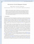
IEEE/ACM Transactions on Computational Biology and Bioinformatics, 2007
Download

Bioinformatics/computer Applications in The Biosciences, 2009
Download
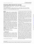
Download

Genome Biology and Evolution, 2011
Download

Bioinformatics, 2013
Download

Lecture Notes in Computer Science
Download

Download

Evolutionary Bioinformatics, 2015
Download
IEEE/ACM Transactions on Computational Biology and Bioinformatics, 2000
Download
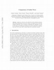
Journal of bioinformatics and computational biology, 2012
Download

International Journal for Parasitology, 2005
Download

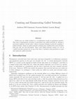
Lecture Notes in Computer Science, 2007
Download
