been published in Oceanography, Volume 17, Number 2, a quarterly journal of The Oceanography Society. Copyright 2003 by The Oceanography Society. All rights reserved. Reproduction of any portion of this artiJune 2004 32This article hasOceanography cle by photocopy machine, reposting, or other means without prior authorization of The Oceanography Society is strictly prohibited. Send all correspondence to: info@tos.org or 5912 LeMay Road, Rockville, MD 20851-2326, USA. From Meters to Kilometers A LO OK AT O CEANCOLOR SCALE S OF VARIABILITY, SPATIAL COHERENCE, AND THE NEED FOR FINESCALE REMOTE SENSING IN COASTAL O CEAN OPTICS B Y W. PA U L B I S S E T T, R O B E R T A . A R N O N E , C U R T I S S O . D A V I S , T O M M Y D . D I C K E Y, D A N I E L D Y E , D AV I D D . R . K O H L E R , A N D R I C H A R D W. G O U L D , J R . Oceanography June 2004 33 INTRODUCTION explicit terms of cost-benefit analysis, such The physical, biological, chemical, and opti- discussions should be integral parts of the (ONR) sponsored the Hyperspectral Coastal cal processes of the ocean operate on a wide scientific design of instruments, platforms, Ocean Dynamics Experiment (HyCODE) variety of spatial and temporal scales, from and experiments aimed at resolving oceanic (Dickey et al., this issue), which presented seconds to decades and from micrometers to processes. the opportunity to study the question of In 2001, the Office of Naval Research thousands of kilometers (Dickey et al., this The practical examples of this problem in issue; Dickey, 1991). These processes drive remote sensing include: “What is the optimal Hyperspectral airborne sensors were de- the accumulation and loss of living and non- repeat coverage frequency?” and “What is the ployed on several platforms at various al- living mass constituents in the water column optimal Ground Sample Distance (GSD) or titudes. This coverage was supplemented (e.g., nutrients, phytoplankton, detritus, sed- pixel size of the data?” For the optical ocean- by numerous space-borne, remote-sensing iments). These mass constituents frequently ographer, there is also the issue of optimal satellites. The airborne instruments included have unique optical characteristics that alter spectral coverage needed to resolve the opti- two versions of the Portable Hyperspectral the clarity and color of the water column cal constituents of interest (Chang et al., this Imager for Low-Light Spectroscopy (PHILLS (e.g., Preisendorfer, 1976). This alteration issue). The sum of these considerations feed 1 and PHILLS 2) (Davis et al., 2002) op- of the ocean color, or more specifically the into the sensor, deployment platform, and erating at an altitude of less than 10,000 change in the spectral “water-leaving radi- deployment schedule decisions. For polar- feet and 30,000 feet, respectively, as well as ance,” Lw(λ), has led to the development of orbiting and geo-stationary satellites that the NASA Airborne Visible/Infrared Imag- optical techniques to sample and study the cost hundreds of millions of dollars, as well ing Spectrometer (AVIRIS) sensor operat- change in biological and chemical constitu- as airborne sensors that have smaller upfront ing at 60,000 feet. These sensors provided ents (Schofield et al., this issue). Thus, these costs but higher deployment costs, the deci- hyperspectral data at 2 m, 9 m, and 20 m optical techniques provide a mechanism to sion of sampling frequency directly impacts GSDs, respectively. The satellite data col- study the effects of underlying biogeochemi- the scientific use of the data stream, and lected included the multi-spectral images cal processes. In addition, because time- and what processes may be addressed with data from Sea-viewing Wide Field-of-view Sensor space-dependent changes in Lw(λ) may be streams collected by these sensors. These (SeaWiFS), Moderate Resolution Imaging measured remotely, optical oceanography scientific cost-benefit analyses extend be- Spectroradiometer (MODIS), Fengyun 1 provides a way to sample ecological interac- yond the cost in dollars because the typical C (FY1-C), Oceansat as well as the multi- tions over a wide range of spatial and tem- lifetime and replacement cycle of these sen- spectral polarimeter Multiangle Imaging poral scales. sors is on the order of years to decades, and SpectroRadiometer (MISR) sensor and sea a poorly designed sensor package is very dif- surface temperature (SST) sensor Advanced ficult to replace. Very High Resolution Radiometer (AVHRR). The question often posed by scientists trying to resolve problems involving the scales of variability in remote-sensing data. These collections provided a wealth of re- temporal and spatial variation of oceanic properties is: “What is the optimal time/ W. Paul Bissett (pbissett@flenvironmental.org) mote-sensing and field data during a spa- space sampling frequency?” The obvious an- is Research Scientist, Florida Environmental Re- tially and temporally intense oceanographic swer is that the sampling frequency should search Institute, Tampa, FL. Robert A. Arnone field campaign, and they offered the ability be one half the frequency of the variation is Head, Ocean Sciences Branch, Naval Research to begin to address the issue of optimal sam- (i.e., Nyquist frequency) of the property of Laboratory, Stennis Space Center, MS. Curtiss pling scales for the coastal ocean. interest. However, therein lies the rub for O. Davis is at Remote Sensing Division, Naval the oceanographer: the range of the relevant Research Laboratory, Washington, DC. Tommy data streams requires the calibration, vali- scales is large, and the range of available D. Dickey is Professor, Ocean Physics Laboratory, dation, and atmospheric correction of the resources and/or actual engineering capa- University of California, Santa Barbara, Goleta, sensor signals to retrieve estimates of Lw(λ), bilities to sample all relevant scales is often CA. Daniel Dye is at Florida Environmental Re- or “remote sensing reflectance,” Rrs(λ), a small. Hence, the decisions affecting re- search Institute, Tampa, FL. David D.R. Kohler is normalized measure of the Lw(λ). Our goals source allocation become critical in order to Senior Scientist, Florida Environmental Research in this paper are to illuminate some of the maximize the total data information in both Institute, Tampa, FL. Richard W. Gould, Jr. issues of remote sensing spatial scaling in quantity and quality. While these scientific is Head, Ocean Optics Center, Naval Research the nearshore environment and attempt to resource decisions are rarely discussed in Laboratory, Stennis Space Center, MS. derive some understanding of appropriate 34 Oceanography June 2004 The use of these multiple remote-sensing sampling scales in the nearshore environ- cube. The calibration of the sensor (Kohler data density is to reduce spectral resolution. ment. We will focus on the data collected by et al., 2002a) and the specific corrections for However, reducing spectral resolution also a single sensor (PHILLS 2) to reduce uncer- the window as well as the atmospheric cor- reduces the biogeochemical information that tainties in the analysis that may result from rection of these data are described elsewhere may be derived from optical data. To look at the different data processing techniques ap- (Kohler et al., 2002b). The data values are the impacts of spectral resolution reduction plied to each of the individual sensors’ data. given in Rrs(λ), units of 1/sr (Mobley, 1994). on the ability to discern spatial variability This single 124-band data cube from July 31, in the spectral Rrs(λ) data, the hyperspectral 2001 represents 15 GB of raw data. This data data were reduced in spectral resolution to was calibrated, atmospherically corrected, approximate the SeaWiFS bands. This was and geo-rectified for the analyses presented accomplished by multiplying the Rrs(λ) by here. the SeaWiFS wavelength response function METHODS The PHILLS 2 was deployed seven times st rd th st st (July 21 , 23 , 27 , 31 a.m., 31 p.m., and st nd August 1 and 2 ) during the 2001 HyCODE LEO-15 field program, and each mission The engineering issues surrounding the (Figure 2). This created an 8-band image, generated nearly 4,000 square kilometers collection, storage, and transmission of with band centers located at 412, 443, 490, of spectral data at 9 m resolution (Figure higher spatial and spectral resolution sys- 510, 555, 670, 765, and 865 nm. These data 1). For this discussion on spatial scaling, we tems are fairly cost intensive. If this image are used to illuminate the different multi- have chosen to focus on a single PHILLS 2 was collected from space, it would require spectral and hyperspectral data streams to image from July 31 , as the coverage pro- over three hours to transmit the data to a resolve information variability in the near- vided by these data approximates the total ground station over an X-band downlink shore environment. spatial extent of a satellite sensor, at a much (for reference, a polar-orbiting satellite has The autocorrelation function has previ- higher spatial resolution, which allows us to approximately an 11-minute transmission ously been used in time-series studies to de- explore scaling issues within a single image window). 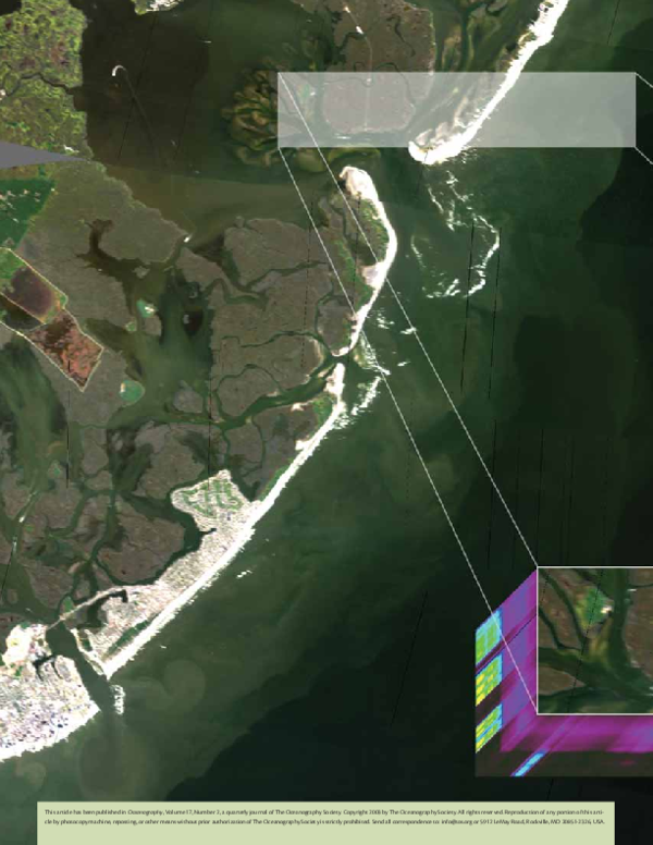One of the easiest ways to reduce termine the optimal time frequency of sam- st Figure 1. A false color composite of the 9 m Portable Hyperspectral Imager for Low-Light Spectroscopy (PHILLS 2) data collected at an altitude of 30,000 feet on July 31, 2001 at the HyCODE LEO-15 study site offshore of New Jersey. The inshore yellow dot represents the location of the LEO-15 profiling bio-optical node. The offshore blue dot is the location of the UCSB OPL (University of California, Santa Barbara, Ocean Physics Laboratory) bio-optical mooring. The inshore small red box and the offshore small green box represent regions of interest (ROIs) where the variance of the SeaWiFS Band 5 Rrs, PC1 (SW) and PC1 (Hyp) were approximately the same, even though the mean was significantly different (see text and Table 1). The size of these boxes represents a mean ground sampling distance (GSD) of 441 m (49 pixels on a side for a total of 2401 pixels equal to approximately 0.2 km2). The white line represents the transect data used in the variable GSD study. Its selection was driven by the desire to use a single flight line of data for the variance calculation (see text). Oceanography June 2004 35 Figure 2. To evaluate the effect of reduced spectral resolution on spatial variability, a reduc- Figure 3. The Simulated SeaWiFS Band 5 Rrs values (sr-1*10,000) along the sampling line tion in the spectral resolution of the hyperspectral data was performed so as to approxi- transect as shown in Figure 1. The vertical green and red lines denote the respective mate that of SeaWiFS bands. Shown are the SeaWiFS wavelength response functions used locations of offshore and inshore regions of interest from which the variance threshold to transform the hyperspectral PHILLS 2 data into a simulated SeaWiFS-type data product. for the GSD analysis was determined. pling (e.g., Abbott and Letelier, 1998; Chang to be different over cross-shore distances would like the scene itself to describe the op- et al., 2002; Dickey et al., 2001), which led compared to along-shore distances. There timal GSD based on the ability of the sensor us to attempt a spatial autocorrelation are other statistical methods for estimating and hyperspectral data to resolve distinct, to examine spatial variability of Rrs(555) spatial variability, including those that de- homogeneous waters. The more rigorous along the transect shown in Figure 1 (Fig- termine the anisotropy in the directionality application of 2-D variance analyses is the ure 3). However, results indicated a trend in of the variance calculation (i.e., the variance subject of a follow-on study. this data record, with higher intensities of is different in different directions) (Curran, Rrs(555) nearshore. Autocorrelation stud- 1988; Dale et al., 2002). Variance ellipses od of estimating spatial variability, one that ies require the mean of any subsample of a have been used to describe the variance in focuses on the ability to separate the linearly record to approximate the mean of the total altimeter-derived velocities in the near- additive noise of the image from the “real” record. Any attempt to calculate a decorrela- shore environment (e.g., Strub and James, geophysical detail of the scene. Linearly ad- tion scale from this transect would result in 2000). Of particular interest may be the use ditive noise refers to the interference derived a value for the decorrelation scale that had a of semivariogram or variograms developed from the noise of the sensor as well as any direct proportional relationship to the total in the soil research community to describe noise generated from the atmosphere or length of the transect. The statistical reason “roughness” in the topology of spatial mea- processing algorithms. If the noise is stable for this is that data from the transect does surements (Curran, 1988). These have been and linear, then the true signal of interest not represent a stationary function (i.e., used with satellite ocean remote-sensing may be retrieved from a sample of a popula- the mean changes as the transect length in- data to describe larger scales of interest in tion, provided the sample size is sufficiently creases and, therefore, the sample variance chlorophyll distributions (e.g., Yoder et al., large. In this case, we would expect that the will increase with domain size) (Chilès and 1987). However, many of these methods standard deviation of the Rrs(λ) signal to be Delfiner, 1999) (see Statistics Review box). require interpretations that are difficult to a proxy for the total noise, and that over any This suggests that the measure (decorrela- definitively relate to geophysical parameters, homogenous region of the scene it should be tion scale) may be an improper statistic to i.e., “sills” and “nuggets” in variograms. Here, constant, regardless of the magnitude of the use to describe the optimal spatial sampling we are interested in determining an optimal signal. Thus, any pixel in a homogenous re- frequency for coastal-ocean data sets. sampling size that is more easily discussed in gion of interest would be equal to the mean terms of this scene of interest and in terms value of the region ± some random compo- of the sensor capabilities. In other words, we nent. While not statistically explored here, the change in mean (and thus, variance) appears 36 Oceanography June 2004 For this study, we derived another meth- background noise-generated standard devia- data to separate water masses into distinct tiplicative noise in our data. Multiplicative tion must contain regions of distinctly dif- optical regions. One approach to using the noise occurs when the noise (i.e., standard ferent optical constituents. full spectrum simultaneously is to first lin- This analysis would fail if there were mul- deviation) is a direct function of the inten- Most studies of spatial variation in radi- early transform the n-dimensional spectral sity (mean) of the signal. By assuming (and ance fields focus on the variance within a data (where n is the number of wavelengths) confirming) that the noise of the scene is single channel, or perhaps a combination into a variance minimizing coordinate sys- truly random and linear, any increase in the of channels. In this study, we wish to assess tem. When the “proper” or root vectors (ei- standard deviation would thus be gener- if there is any additional information to be genvectors) of this new coordinate system ated by a change in real geophysical proper- retrieved from the continuous spectrum of are orthogonal to each other, this type of ties within the region of interest. Therefore, reflectance data, as opposed to using only transformation is called a Principal Com- an increase in a region’s standard deviation one or two bands individually. The question ponent Analysis (PCA). A PCA allows the above a background random noise-gener- of how to use the entire hyperspectral data user to focus on the vectors that describe the ated standard deviation would suggest a simultaneously to identify homogeneous most variance (information) using the entire nonhomogenous region of interest, i.e., one regions of optical properties is an active area spectral and image space, rather than focus- with real differences in the region’s geophysi- of research; as a first step, we would like to ing only on the variance in the image at a cal properties. Put simply, a region of inter- be able to determine if the full spectrum of- single wavelength A PCA is a powerful way est with a standard deviation greater than a fers any ability over single or multichannel to look for patterns. S TAT I S T I C S R E V I E W When analyzing any data set, a good place to start is data sets, one would expect 68 percent of the popula- Other measures, such as sample variograms and by calculating the data set’s mean (a measure of the tion to fall with 1 standard deviation (1σ) around the Pair Quadrat Variance (PQV), focus only on the change central tendency) and variance (a measure of the dis- population’s mean. The probabilities that any member with lag distance. For a transect of n contiguous or persion or variability). The mean is given by the fol- of the population would fall within 2 and 3σ are ap- equally spaced intervals (quadrats), a sample variogram lowing equation: proximately 95 and 99 percent, respectively. for a given distance d is given by (Dale et al., 2002): n ∑X µ= n−d In spatial data analysis, one is frequently interested i in how a sample at one spot co-varies or correlates i =1 N γˆ ( d ) = with the same measure of a sample in another location. ∑( X i − Xi + d ) 2 i =1 N −d where the capital Greek letter sigma (Σ) means sum- Autocovariance and autocorrelation are simply mea- mation over all values, Xi, in the population, divided by sures of the covariance and correlation of the values of sample variogram is constant with respect to direc- the total number of values, N, in the population. The a single variable for all pairs of points separated by a tion, it is referred to as isotropic. If the variogram variance is given by: given spatial lag (Dale et al., 2002). An estimate of the changes with respect to the direction with which it autocovariance for samples at a distance d is given by: was calculated, then it is referred to as anisotropic. It n σ2 = ∑( X i − µ) 2 n−d ∑( X i =1 N It is easily seen that the greater the separation of the individual values, Xi, are from the mean, , the Cov = i − µ ) ( Xi + d − µ ) i =1 N −d The autocorrelation is given by dividing Cov by σ2. Note that this equation is omnidirectional. If the is clear from Figures 1 and 6 that there appears to be a directionality component to the along shore and cross shore variance, and thus this image would be consider anisotropic. larger the variability of the population represented in The value of these statistics in describing the data set of the data set grows. The square root of the variance is interest depends on the validity of the underlying as- REFERENCE S called the standard deviation. When the population is sumptions. A trend in the spatial data (similar to Figure Dale, M.R.T., P. Dixon, M.-J. Fortin, P. Legendre, D.E. Myers, normally distributed around its mean, the standard de- 3) violates the assumption of stationarity, i.e. the esti- and M.S. Rosenberg, 2002: Conceptual and mathemati- viation provides a measure that is easily conceptualized mate of the mean and the autocorrelation are constant cal relationships among methods for spatial analysis. as a distance away from the mean. The standard devia- with respect to distance along the record, and negates Ecography, 25, 558-577. tion may also be used to produce a confidence interval the effectiveness of the autocovariance and autocorre- in populations that are normally distributed. In such lation in the overall analysis. Oceanography June 2004 37 It should be noted that great care must the user to recognize that it is a hyperspec- eigenvalues of the first eigenvector created be used in analyzing a PCA transformation tral vector itself, which could not have been from a PCA (referred to as PCA Hyp) of the of a hyperspectral image. There will be an generated without the full spectral data set. hyperspectral image. We used the Environ- equal number of eigenvectors as there are The easiest way to see the impacts of all of ment for Visualizing Images (ENVI) soft- spectral channels, but frequently only the the wavelengths on the eigenvector is to ware package from Research Systems, Inc., to first 10 eigenvectors are necessary to de- square the PCA eigenvectors to calculate accomplish a PCA of the hyperspectral data. scribe >99 percent of the total variance in each channel’s percentage contribution to The first eigenvector (PC1) of both the hy- the scene. However, the number of eigenvec- the description of scene’s spectral variation. perspectral and two band images described tors needed to describe the total variance in We seek to use the hyperspectral data to >95 percent of the variance of the images; the scene is completely image dependent. If separate homogenous water masses, and we PCA Hyp PC1 = 95.6 percent and PCA SW there is a large amount of spectral variation believe that there is additional information PC1 = 99.0 percent. The second and third ei- in the scene, then more eigenvectors will in the full spectrum of the radiance field, genvector of the PCA Hyp accounted for 2.9 be needed to describe the majority of the rather than in any single channel or combi- percent, and 0.7 percent of the image’s spec- scene variance. If there is a small amount of nation of channels. In order to test this be- tral variance, respectively. The total variance spectral variation, then a smaller number of lief, we will compare the spatial variability of described by the remaining eigenvectors for eigenvectors will be required. As an example, three images created from the same hyper- PCA Hyp is 1.43 percent. There are only two many open-ocean images have been found spectral data set. The first image is a single eigenvectors for the PCA SW, and the second to only need the first three eigenvectors to simulated SeaWiFS band (Band 5). The sec- accounts for 1 percent of the variance. The first three eigenvectors from the PCA describe 98 percent of the scene dependent ond is an image of the eigenvalues of the first variance (e.g., Mueller, 1976). For these eigenvector created from a PCA (referred Hyp as well as the percentage contribution ocean images, a common error in PCA is to to as PCA SW) of a simulated two band from each spectral channel to each eigen- assume that only three spectral channels are SeaWiFS image (Bands 3 and 5). These two vector, is shown in Figure 4. It is clear that needed to describe the scene dependent vari- bands were selected for this multispectral while there are some dominant channels in ance. It must be understood that the eigen- test, since they are used in many common the first eigenvector (i.e., approximately 560 vector is a measure of the variance across all SeaWiFS chlorophyll algorithms (O’Reilly et nm in PC1), it peaks at only approximately bands simultaneously, and therefore requires al., 1998). The third image is an image of the 6 percent, which means that the other wave- A B Figure 4. So as to evaluate the entire spectral data set, Principal Component Analysis (PCA) was used to reduce the dimensionality of the image. PCA is a method of maintaining nearly all of the characteristics of the original data set while reducing the number of parameters needed to describe the data. This is accomplished by reprojecting those data along orthogonal axes that are positioned to best describe the variance of the data (eigenvalues and eigenvectors). The first three eigenvector principal components are displayed in (A). The influence that each spectral band had on the first three principal components is displayed in (B). 38 Oceanography June 2004 lengths contribute 94 percent of the influence on the variance described by this vector Image Type Region of Interest, ROI Mean of ROI Standard Deviation of ROI Inshore 52.77 1.54 Offshore 24.55 1.85 Inshore 13.38 1.79 Offshore -21.68 1.98 Inshore 111.08 6.44 Offshore -12.11 7.46 (Figure 4A). Therefore, it would not be accurate to say a single channel would describe Simulated SeaWiFS Band 5 95.6 percent of the variance in this image. A more accurate statement would be that the spectral shape that describes the most variance in this image is demonstrated in the PC1 of Simulated SeaWiFS Bands 3 and 5 PC1 of Hyperspectral Cube first eigenvector. Two regions of interest (ROIs) in the visually homogenous areas of the imagery Standard Deviation Used in Analysis, σt 2.0 2.2 8.0 Table 1. The mean and standard deviation from the simulated single-band image (SeaWiFS Band 5) as well as the first Principal Component Analysis eigenvalue images from simulated dual band (SeaWiFS Band 3 and 5), and hyperspectral data. Also, included is the test standard deviation, σt, used for the optimal GSD calculation. were selected to confirm the hypothesis of linear noise (which should be applicable to the PCA because it is a linear transformation of the hyperspectral data) and to gen- rections, while remaining centered on pixel differences, probably resulting from the erate a test standard deviation value. These i, and the mean and standard deviations sediments suspended during the passage of two ROIs were approximately 441 m on a were recalculated. This procedure continued the weather front. This variability is repre- side (49 pixels), (approximately 0.2 km , until σi was greater than σt, at which point sented in Figure 6, as a false color composite 2401 pixels); one region was inshore while the size of the previous non-failing ROIi was of the PCA Hyp PC1 eigenvalues rendered the other was offshore (Figure 1). Table 1 recorded. The size of the ROIi should then in density slices. Clearly, there is a tremen- gives the mean and standard deviations for equate to the maximum size of a region with dous amount of spatial variability inshore, the two ROIs from the simulated SeaWiFS homogenous optical properties. which decreases as we move offshore. As we 2 move offshore past 20 km, the optimal GSD Band 5 as well as the PC1 for PCA SW and PCA Hyp. Note this standard deviation is RE SULTS AND DISCUSSION increases for each test. However, beyond not normalized by the mean (e.g., Mahade- The results of this approach in describing this point there are significant differences van and Campbell, 2002; Mahadevan and the spatial variability of this coastal environ- between the SW Band 5 and PCA SW and Campbell, in press) because we are trying ment may be found in Figure 5. Here, the the PCA Hyp. The optimal average GSD to separate random noise of the sensor and largest GSD of the ROIi that has a standard and median GSD grow to approximately 2 processing from the real geophysical changes deviation greater than or equal to σt is plot- km and approximately 1.5 km, respectively, in the image. Theoretically, any homogenous ted as a function of the position along the for SW Band 5 as the water masses become region of the same size should have a similar transect for three images: single band (Fig- more homogeneous with respect to this standard deviation; otherwise, some real fea- ure 5A), dual band PC1 (Figure 5B), and wavelength. The average and median GSD ture of interest has been included within the hyperspectral PC1 (Figure 5C). It can be for the PCA SW and PCA Hyp are less, as study region. As the ROIs were selected with seen that the size of the GSD increases when the additional bands of information provide an eye to a perfectly homogenous region, we moving from onshore to offshore. The opti- improved ability to delineate water-mass allow for some error in our selection criteria. mal GSD for each data set increases rapidly types. There is some additional geophysical Table 1 also provides the test standard devia- out of the surf zone to an average of approx- structure between 28 and 40 km that reduces tion, σt, for each of the GSD calculations. imately 100 m within 200 m of the shore. By the optimal GSD back to the levels seen about 10 km, the optimal GSD grows to >1 nearshore for all three tests. Once offshore (Figure 1), a new ROIi was created with a km. The average and median optimal GSD more than 40 km, the optimal GSD grows to minimum size of 3 X 3 pixels, or 27 X 27 m for all vary between 150 and 200 m out to > 6 km for the Band 5 test, and > 4 km for (729 m ). The mean and standard deviation, 5 km, with the average GSD growing to ap- the PCA SW. These larger GSDs approach σ, of each region was calculated, and σi was proximately 1 km beyond approximately 12 the scale of chlorophyll distributions de- compared against σt. If σi was less than σt, km from the shoreline. scribed by others in the coastal environment Next, at every pixel along the transect line 2 then ROIi increased in size by two pixels in The variability inshore for each GSD each of the along-track and cross-track di- calculation is driven primarily by intensity using multispectral data (e.g., Yoder et al., 1987). However, the PCA Hyp drops back to Oceanography June 2004 39 A B Figure 5. (A) To determine the optimal GSD for the SW Band 5 Rrs, the real geophysical variation along the flight line transect needed to be resolved. The data values show that nearshore (<10 km) C an optimal GSD would be less than 100 m to 200 m. These optimal GSDs grow to 1 km farther offshore. Note, however, that there are discontinuities in the progression of larger and larger GSDs as one moves offshore. This may suggest the crossing of a frontal boundary, which would require a smaller GSD to resolve. The blue and red lines are the mean and median, respectively, of the GSDs from a particular point along the transect to the most inshore point. The vertical green and red lines denote the respective locations of the inshore and offshore regions of interest (ROIs) from which the variance threshold for the GSD analysis was determined. The horizontal grey line indicates the size of the region of interest from which the threshold was determined. (B) Determining the optimal GSD for the simulated SeaWiFS PC1 image was accomplished in the same manner as Figure 5A. Similar to Figure 5A, this figure illustrates the same basic trend: smaller GSDs are required inshore while larger GSDs are sufficient off shore. The description of the lines in the image are the same as in Figure 5A. (C) The optimal GSD for the hyperspectral PC1 image was determined in the same manner as Figure 5A. In shore, this analysis is in agreement with the results from the other two GSD studies. However, offshore the variance found within the PC 1 (Hyp) was significantly greater than what was witnessed in the other two studies resulting in smaller GSDs required to resolve what were thought to be regions of homogeneous ocean color. The description of the lines in the image are the same as in Figure 5A. Figure 6. A false color composite of the inshore variability of the GSD is shown. The image displays the eigenvalues associated with the first eigenvector of the PCA Hyp (PC1) image generated from the hyperspectral data. The eigenvalues are mapped into linear density slices and colored using a linear blue to red color table. A land mask was applied prior to the PCA being applied to the data set. Results suggest that the variability of the 40 Oceanography June 2004 water color is greater as one approaches the shore. levels seen nearshore, suggesting the hyper- boundary). In addition, the input of fresh signals may be a function of the total num- spectral data offers additional information water has its greatest impact on baroclinic- ber of bands sampled. with which to separate features in otherwise ity in the nearshore environment. The use of homogeneous-appearing waters. optical tracers for salinity (Coble et al., this data set of interest by rotating the coordi- issue) may actually improve the understand- nate system into one that minimizes the confirm what many coastal oceanographers ing and prediction of coastal circulation, a variance across the entire data space. In intuitively understand. The closer to shore requirement for any study on the sources the hyperspectral image cube of Figure 1, a one approaches, the more variable the color and fate of biogeochemically relevant mate- single eigenvector (Figure 4) accounts for of the water. In the optically deep waters off rials. These results suggest that color studies most of the variance in this image. While the coast of New Jersey, the optical features at the LEO-15 site may require GSDs ap- this eigenvector (PC1) may appear similar to are driven by the wind and tidal mixing of proximately 100 m to resolve biogeochemi- a water-leaving radiance vector in high-scat- sediments as well as allochthonous inputs cal processes from ocean-color data. tering green waters, great care must be used In many respects, these statistical results A PCA reduces the dimensionality of a of sediments, nutrients, and organic mate- The optimal GSD is also a function of in ascribing real geophysical properties to rial from rivers and estuaries. In addition, the information content of the data set. The eigenvectors. Figure 4B does show why the far field dynamics drive coastal jets that also single-band data set shows less variability in three techniques were so similar, particularly bring in allochthonous material into this lo- its standard deviation than the PC1 of the in the nearshore region, as the wavelengths cation (Chant et al., in press), which are tid- dual-band data set, which in turn shows less around 560 nm influenced the variance of ally mixed with nearshore waters. This drives variability in the standard deviation than the the PC1 the most. PCA is a tool to describe the variability of the optical signal to a very PC1 of the hyperspectral data set. This effect scene-dependent variance, and in this pa- high level over small spatial distances. As we results in lower mean and median optimal per, we focus on the information content move offshore into the deeper waters of the GSDs as the number of bands used in the of spectral data over small homogeneous shelf, the impacts of tidal oscillations are less analysis increases. This result suggests that regions of water color, and intensity across important. The change in water-mass optical additional bands add information that may a large scene of interest. The spatial scale characteristics is driven by the interactions be used to discriminate optically different of homogeneous regions often depends on of larger-scale physical features (i.e., mean water masses, and perhaps retrieve estimates the total number of bands used to describe currents) and weather patterns. These larger- of different optically active constituents. that homogeneous region, particularly when scale processes tend to homogenize water In particular, beyond 40 km, there is a real moving away from the shallow water regions masses over kilometer scales, and as a result, divergence between the GSDs of the PCA impacted by high-energy mixing. It does the GSD needed to adequately resolve the Hyp and those derived from the simulated not, however, necessarily suggest that eco- real horizontal geophysical boundaries with- SeaWiFS data set. Unsurprisingly, it also sug- logical parameters of interest vary over these in these homogenous waters grows in size. gests that the optimal GSD for delineating same scales. The determination of variance the spectral variances in upwelling radiance of ecological-relevant material would In the nearshore environment (less than 10 km from the shore in this example), each of these tests yield approximately the same result (Figure 7). It would appear from this result that to adequately describe the geo- Figure 7. The inshore GSD for SW Band 5, PCA SW, and PCA Hyp. The physical features in the nearshore, the GSD similarity within this region of the must be < 200 m. Many important bio- GSD trends is striking, and suggests chemical processes occur within 10 km of that variance within the inshore region may be driven by the concen- the shore. River discharges of nutrients and trations of suspended matter. The organic matter have their greatest influences vertical red line denotes the loca- in this nearshore region, and the cycling of tion of the inshore ROI from which the variance threshold for the these materials within the nearshore envi- analysis was determined. The hori- ronment may have large impacts on esti- zontal grey line indicates the size of mates of the fate of biogeochemical elements the region of interest from which the threshold was determined. (e.g., carbon, at the terrestrial or ocean Oceanography June 2004 41 depend greatly on the algorithms that in- the ROIs shown in Figure 1, the Band 3:5 1999; Lee and Carder, 2004; Louchard et al., vert color and intensity into optically active ratio showed a significant difference in stan- 2003; Mobley et al., 2002). In addition, hy- mass constituents (i.e., chlorophyll, colored dard deviation, versus the similar standard perspectral approaches may also yield infor- dissolved organic matter [CDOM], sedi- deviations calculated for each band in each mation on phytoplankton speciation, which ments). ROI. This violates our primary assumption, might allow for the remote identification of Ocean-color research and applications are and suggests that studies using ratio analyses harmful algal blooms (HABs) (Roesler et frequently more concerned with the prod- should attempt to delineate the differences al., in press). These hyperspectral imagery ucts derived from Rrs(λ) estimates (e.g., total in the variances of biogeochemical estimates analysis techniques offer the potential to absorption, total scattering, diver visibility, that result from variance of the data versus dramatically increase our ability to retrieve total chlorophyll concentration), rather than the mathematical variance created by the ap- coastal zone information from ocean color the Rrs data itself. It may be that the appro- plication of the algorithm. data streams and specifically address critical priate spatial sampling frequency for these This work suggests that future studies on issues in coastal-zone management. As we products is different than the sampling fre- the optimal sampling frequency in the spa- move from multispectral to hyperspectral quency determined from the spatial varia- tial domain of remote-sensing data begin data products, we may also find a need for tions in the radiance fields. However, using with the Rrs data itself. Furthermore, the op- higher spatial resolution data to better de- the products produced from these same timal sampling frequency may be a function scribe the changes in the nearshore coastal radiance fields to determine spatial sam- of the total number of wavebands available environment. pling frequencies may produce vary different for analysis. This work does not definitively scaling results, strictly due to the method of suggest that variations of optically-active SUMMARY AND CONCLUSIONS product generation. In this paper, we show constituents may be retrieved at the same There are probably many methods of de- how the noise of the sensor and atmospheric spatial resolution as the variation in the total termining the optimal spatial sampling fre- processing approximates a linear transform Rrs vector. However, it does suggest that spa- quency in the coastal zone. However, when function, and we expect that the variance in tial variations in ocean color depend on the a statistical approach is used, care must be radiance data above the background linear number of channels used to described differ- taken to use a method that is applicable to noise represents true difference in ocean col- ences between homogenous regions. If these the sample, and to ensure the rigorous as- or. However, many remote-sensing product additional channels can be used to discrimi- sumptions of stationary functions are not calculations are nonlinear transforms of the nate additional biological, chemical, and violated. Otherwise, unclear results are ob- Rrs data (e.g., Lee and Carder, 2002; O’Reilly physical information, then the hyperspectral tained that may lead to an inefficient scien- et al., 1998). A nonlinear transform of the ocean color signal will yield a greater ability tific design of a remote sensing sensor or ex- Rrs data will alter the mean and variance sta- to identify, study, and predict important eco- periment, for example, for the data discussed tistics in ways that may alter scaling results logical processes in the coastal environment. here, the assumptions inherent to using the New algorithms are being developed that autocorrelation function were violated, in- focus on relatively continuous spectral data dicating that autocorrelation analysis is the sis using a ratio of a simulated Band 3 to rather than on the ratio of multispectral wrong tool for this coastal data set. Band 5 because our primary assumption is channels. These new algorithms use a variety The results described here suggest that the that the sum of environmental and sensor of techniques to take advantage of the great- spatial resolution required for offshore stud- noise is a linearly additive component of the er degrees of freedom that the hyperspec- ies may be dependent on the spectral resolu- total signal, and the standard deviation of tral data stream offers to the ocean-color tion of the data stream. At LEO-15 between this noise component of the signal would scientist; algorithms are in development to 1 and 10 km, a 50- to 200-m GSD appears be constant across varying levels of inten- retrieve standard oceanographic products, sufficient for single-band, dual-band, and sity. If this assumption is true (and it would such as total chlorophyll and CDOM, as well hyperspectral-band data. Within 1 km of appear so from this analysis), then a linear as new products such as bathymetry, bottom the shore, an even higher resolution sensor addition of noise to a downward trending type, and water-column Inherent Optical might be needed to resolve the wind and tid- numerator would yield an increasing vari- Properties (IOPs) (e.g., Dierssen et al., 2003; ally impacted features. In the optically deep ance estimate of a ratio product. In fact, for Hoge et al., 2003; Lee et al., 1998; Lee et al., offshore waters of LEO-15, bottom effects do shown here. We specifically did not include an analy- 42 Oceanography June 2004 not impact Rrs. However, in optically shallow ACKNOWLED GEMENTS areas, the spatial heterogeneity of the bottom This work was supported by the Office of may further reduce the GSD required to re- Naval Research. We would like to thank Sha- solve the optical constituents near the coast ron DeBra and Mubin Kadiwala for their (see Philpot et al., this issue). Offshore of 10 help in editing and preparing this paper. km, there is a significant difference in the Lastly, the review and comments of Dr. Ri- ability to discriminate optical boundaries cardo Letelier were greatly appreciated. using the single or dual band data compared to the hyperspectral data. This suggests that REFERENCE S hyperspectral data may be better able to de- Abbott, M.R., and R.M. Letelier, 1998: Decorrelation scales of chlorophyll as observed from bio-optical drifters in the California Current. Deep Sea Research II, 45, 1,6391,667. Chang, G.C., T.D. Dickey, O.M. Schofield, A.D. Weidemann, E. Boss, W.S. Pegau, M.A. Moline, and S.M. Glenn, 2002: Nearshore physical processes and bio-optical properties in the New York Bight. Journal of Geophysical Research, 107(C9), 3,133. Chant, R.J., S. Glenn, and J. Kohut, in press: Flow reversals during upwelling conditions on the New Jersey inner shelf. Journal of Geophysical Research. Chilès, J.-P., and P. Delfiner, 1999: Geostatistics: Modeling Spatial Uncertainty. John Wiley and Sons, Inc., New York, 720 pp. Curran, P.J., 1988: The semivariogram in remote sensing: An introduction. Remote Sensing of Environment, 24(3), 493-507. Dale, M.R.T., P. Dixon, M.-J. Fortin, P. Legendre, D.E. Myers, and M.S. Rosenberg, 2002: Conceptual and mathematical relationships among methods for spatial analysis. Ecography, 25, 558-577. Davis, C.O., J. Bowles, R.A. Leathers, D. Korwan, T.V. Downes, W.A. Snyder, W.J. Rhea, W. Chen, J. Fisher, W.P. Bissett, and R.A. Reisse, 2002: Ocean PHILLS hyperspectral imager: Design, characterization, and calibration. Optics Express, 10(4), 210-221. Dickey, T., S. Zedler, X. Yu, S.C. Doney, D. Frye, H. Jannasch, D. Manov, D. Sigurdson, J.D. McNeil, L. Dobeck, T. Gilboy, C. Bravo, D.A. Siegel, and N. Nelson, 2001: Physical and biogeochemical variability from hours to years at the Bermuda Testbed Mooring site: June 1994 March 1998. Deep Sea Research II, 48, 2,105-2,140. Dickey, T.D., 1991: The emergence of concurrent high-resolution physical and bio-optical measurements in the upper ocean and their applications. Reviews of Geophysics, 29(3), 383-413. Dierssen, H., R. Zimmerman, R. Leathers, T. Downes, and C. Davis, 2003: Ocean-color remote sensing of seagrass and bathymetry in the Bahamas Banks by high-resolution airborne imagery. Limnology and Oceanography, 48(1, part 2), 444-455. Hoge, F.E., P.E. Lyon, C.D. Mobley, and L.K. Sundman, 2003: Radiative transfer equation inversion: Theory and shape factor models for retrieval of oceanic inherent optical properties. Journal of Geophysical Research, 108(C12), 3,386. Kohler, D.D.R., W.P. Bissett, C.O. Davis, J. Bowles, D. Dye, J. Britt, J. Bailey, R. Steward, O.M. Schofield, M. Moline, S. Glenn, and C. Orrico, 2002a: Characterization and calibration of a hyperspectral coastal ocean remote sensing instrument. In: Proceedings of the AGU/ASLO Ocean Sciences 2002 Meeting, Honolulu, HI, February 11-15. American Geophysical Union, Washington, D.C. lineate optically distinct regions in offshore coastal waters and that scaling studies may be dependent on the total number of spectral channels used in the analysis. Nonlinear transforms of Rrs, typical of algorithms for products such as chlorophyll concentration, may alter variance calculations; optimal scaling results for these derived products may depend in part on the transform of the data, or the algorithm used. Care must be used when deriving statistics on nonlinear transforms to avoid missing real differences in ocean color and biogeophysical boundaries. The real goal in optical oceanography is to use optics to identify interesting oceanic features as well as describe their time-dependent change. These features range from individual, HAB-forming phytoplankton species to the delineation of terrestrial outflow plumes from background coastal waters. The features may also include bottom characteristics, such as seagrass beds or coral formations. The future of hyperspectral imagery will depend on the ability to retrieve these optically distinct constituents from the Rrs(λ) data streams. One of the first steps in retrieving biogeochemical information from imagery data is to resolve the spatial variations distinguishable in these hyperspectral scenes. The next step will be to focus on the development of new algorithms that use the entire water-leaving spectrum to assess and monitor the coastal zone environment. Kohler, D.D., W.P. Bissett, C.O. Davis, J. Bowles, D. Dye, R.G. Steward, J. Britt, M. Montes, O. Schofield, and M. Moline, 2002b: High resolution hyperspectral remote sensing over oceanographic scales at the LEO 15 field site. In: Ocean Optics XVI, conference held in Santa Fe, NM, November 18-22. Office of Naval Research, Washington, D.C. Lee, Z., K.L. Carder, C.D. Mobley, R.G. Steward, and J.S. Patch, 1998: Hyperspectral remote sensing for shallow waters: 1. A semianalytical model. Applied Optics, 37(27), 6,329-6,338. Lee, Z., K.L. Carder, C.D. Mobley, R.G. Steward, and J.S. Patch, 1999: Hyperspectral remote sensing for shallow waters: 2. Deriving bottom depths and water properties by optimization. Applied Optics, 38(18), 3,831-3,843. Lee, Z.P., and K.L. Carder, 2002: Effects of spectral band numbers on the retrieval of water column and bottom properties from ocean color data. Applied Optics, 41(12), 2,191-2,201. Lee, Z.P., and K.L. Carder, 2004: Absorption spectrum of phytoplankton pigments derived from hyperspectral remote-sensing reflectance. Remote Sensing of Environment, 89, 361-368. Louchard, E., R. Reid, F. Stephens, C. Davis, R. Leathers, and T. Downes, 2003: Optical remote sensing of benthic habitats and bathymetry in coastal environments at Lee Stocking Island, Bahamas: A comparative spectral classification approach. Limnol. Oceanogr., 48(1, part 2), 511-521. Mahadevan, A., and J.W. Campbell, 2002: Biogeochemical patchiness at the sea surface. Geophysical Research Letters, 29(19), 1,926. Mahadevan, A., and J.W. Campbell, eds., in press: Biogeochemical variability at the sea surface: How it is linked to process response times. Pp. 215-226 in Handbook of Scaling Methods in Aquatic Ecology: Measurement, Analysis, Simulation. CRC Press, Boca Raton, FL. Mobley, C.D., 1994: Light and Water. Academic Press, San Diego, CA, 592 pp. Mobley, C.D., L. Sundman, C.O. Davis, M. Montes, and W.P. Bissett, 2002: A look-up-table approach to inverting remotely sensed ocean color data. In: Ocean Optics XVI, conference held in Santa Fe, NM, November 18-22. Office of Naval Research, Washington, D.C. Mueller, J.L., 1976: Ocean color spectra measured off the Oregon coast: Characteristic vectors. Applied Optics, 15(2), 394-402. O’Reilly, J.E., S. Maritorena, B.G. Mitchell, D.A. Siegel, K.L. Carder, S.A. Garver, M. Kahru, and C. McClain, 1998: Ocean color chlorophyll algorithms for SeaWiFS. Journal of Geophysical Research, 103, 24,937-24,953. Preisendorfer, R.W., 1976. Hydrologic Optics, Volumes 1-6, National Oceanic and Atmospheric Administration, Honolulu, Hawaii. NTIS PB-259 793. National Technology Information Service, Springfield, VA, 1,727 pp. Roesler, C.S., S.M. Etheridge, and G.C. Pitcher, in press: Application of an Ocean Color Algal Taxa Detection Model to Red Tides in the Southern Benguela. In: Proceedings of the Tenth International Conference for Harmful Algal Blooms. Strub, P.T., and C. James, 2000: Altimeter-derived variability of surface velocities in the California Current System: 2. Seasonal circulation and eddy statistics. Deep Sea Research II, 47, 831-870. Yoder, J.A., C.R. McClain, J.O. Blanton, and L.Y. Oey, 1987: Spatial scales in CZCS-chlorophyll imagery of the southeastern U.S. continental shelf. Limnol. Oceanogr., 32(4), 929-941. Oceanography June 2004 43