2010 7th Intenational Multi-Conference on Systems, Signals and Devices A Rule-Based System for Trajectory Planning of an Indoor Mobile Robot Siba M. Sharef, Waladin K. Sa'id, Farah S. Khoshaba Control and Systems Engineering Department, UO, Iraq. Siba sharef@yahoo.com waladinksy@yahoo.com farah_sami76@yahoo.com Ahstract- In this developed for a controller unknown that paper, two can a navigate environment. sotware wheels The driven the work simulation mobile robot safely involves model robot the is motion through design an of a controller, which has four functions: motion control; obstacle avoidance; self-location; and path planning both global and local. The proposed controller is responsible for the mobile robot navigation ater it generates a trajectory between start and goal points. Also it enables the robot to operate successfully in the presence of various obstacles present in any user built maps. The mobile robot is able to locate its position on any given map. The dynamic of the mobile robot is examined and the time constant of the two motors, which affects the direction of the mobile robot motion, is controlled. Obstacle avoidance is implemented with Fuzzy Logic Controller. The numerical experiments demonstrated that the indoor robot navigated successfully in tight corridors, avoided obstacles and dealt with a variety of world maps with presented to it. various 1. irregular wall shapes that were INTRODUCTION Automated Guided Vehicle (AGV) has been in existence since the 1950's. AGVs are driver-less industrial trucks, usually powered by electric motors and batteries and were applied mainly in warehouses, factories and mines [I]. Since then mobile robots were developed and applied in factories, military, planetary exploration, mining, woods, hospitals and for the disabled. The advancement in technology and in particular the development of on-board signal and data processng technology has added to the acceptance and wide spreading of its use. A wheeled mobile robot is a wheeled vehicle, which is capable of an autonomous motion (without extenal human driver) because it is equipped, for its motion, with sensors and actuators that are driven by an embarked computer [2]. They come in a variety of sizes, shapes, and capabilities, but they are all made up of the same important parts; each of these parts must be designed to work with other parts of the system as well as the other machines in a work cell [3}. One of the most important tasks in autonomous navigation is to create a suitable path planning in environments where robot navigates [4]. In moving between two points, the mobile robot must plan its path (globally and locally) as well as avoiding obstacles by temporarily deviating rom the planned path. Furthemore, robot motion must be controlled which implies the strategy by which the platform approaches a desired location and the implementation of this strategy [5]. The robot should be capable of intelligent motion and action 978-1-4244-7534-6/10/$26.00 ©201O IEEE without requiring any extenal support while executing a given task. There are many algorithms for control of mobile robots described in literature [6]. However control of nonholonomic systems is a dificult problem. In tasks such as trajectory tracking or following a predetemined trajectory, it is necessay to control simultaneously the position and orientation of the robot, as well as its velocity. This paper focuses on the application of FLC to move, orient and avoid obstacles of a mobile robot as it navigates in an indoor environment. For this end a differentially wheel driven mobile robot is considered and its kinematics and dynamics are modeled and the control action of the wheels speed is discussed. Global and local path planning and localization method are also examined and simulated. II. 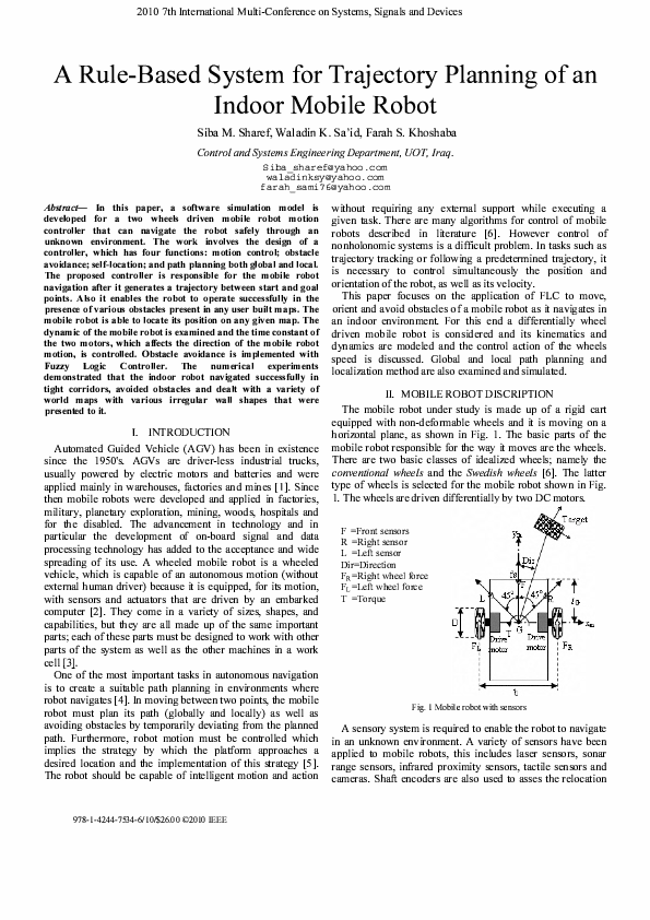MOBILE ROBOT DISCRIPTION The mobile robot under study is made up of a rigid cart equipped with non-deformable wheels and it is moving on a horizontal plne, as shown in Fig. 1. The basic parts of the mobile robot responsible for the way it moves are the wheels. There are two basic classes of idealized wheels; namely the conventional wheels and the Swedish wheels [6]. The latter type of wheels is selected for the mobile robot shown in Fig. 1. The wheels are driven differentially by two DC motors. F =Front sensors R =Right sensor L =Let sensor Dir=Direction FR =Right wheel force FL =Let wheel force T =Torque Fig. 1 Mobile robot with sensors A sensory system is required to enable the robot to navigate in an unknown environment. A variety of sensors have been applied to mobile robots, this includes laser sensors, sonar range sensors, inrared proximity sensors, tactile sensors and cameras. Shat encoders are also used to asses the relocation 2010 7th Intenational Multi-Conference on Systems, Signals and Devices of the robot in comparison with the previous cycle. Furthemore, they are used to estimate the thereabouts of the robot position relative to the starting point or the borders of the environment while the robot navigates in the environment [7]. Fig. 1 shows the proposed sensor layout for the mobile robot under study. The igure shows three sonar sensing devices mounted in ront, let and right of the robot's platform. : oom: : :....... : ...�... ;.��.. �t�. 7�I Yo .;+ _� .' -" -_-._: ) o .. � ... ____ i '.���._� .. ....... � _____ ... t Fig. 2 Mobile robot in a typical indoors space The position of the robot in the plane is described by the ixed rame (xo,yo,zo) and the moving coordinates system (xm,Ym,zm), as shown in Fig. 2. The rame (xo,Yo,zo) is located at any convenient point in the buildng and the moving rame (xm,Ym,zm) is ixed at point G in the platform. The robot posture can be described in terms of the orign of rame (xm,Ym,zm) and its orientation angle > (Fig. 2) both with respect to the base rame with origin at O. III. MODELING of the MOBILE ROBOT The kinematics and dynamics of the 2-DOF differentials drive vehicle shown in Fig. 1 is given in this section. The analysis assumes that the contact between the wheel and the ground is reduced to a sngle pont of the plane. The purpose of kinematics is to deine the relationship between all known or measurable positions and velocities, and all quantities, which are computed by kinematics. With reference to Fig. 1 and Fig. 2, the linear velocity vector for the centre point of the differential-drive mobile robot is given by; VG c �s > c s> c �s> V G = =. � YG VGSll> 2 Sll> Sll> VR [� ] [ ] [ [� = D c s> c �s> 4 Sll> Sll> ] [ L] ] [OORL] b c> + 2LG s> D =- b s>-2LG c> 4b -2 P And the position vector is, = .. : 3 [�Yffssl [ [�::] � M[:�] --. : oom . To construct workable system trajectories, the differential kinematics are required for point "fs" on the mobile platform. This point is the base of the ront sonar sensor. Simple analysis shows that this differential kinematics is described by the following position/orientation vector [8]; (1) As shown in Fig. 2, V G is the linear velocity of the robot's centre (point G) along axis xm. VL and VR are the velocities of the let and right side wheels, respectively. Similarly, the wheels angular velocities are iL and iR and D is the wheel diameter. xG and YG are the robot's velocity components along the ixed rame coordinates (xo,yo). The orientation of the robot expressed by > is obtained by dividing the rows of equation (l), i.e., >=tan' \ xG /YG) ' (2) M (3) The value of the elements of matrix follows directly rom equation (2). The symbols c and s have been used instead of cos and sin. Equation (2) shows that the output velocities are nonzero even if only one wheel is rotating. For this reason this type of platform has the ability to change its orientation on the spot. Mobile robot dynamics refer to the relationship between forces, torques and acceleration. Applying Newton's second law of motion to the differential-drive mobile robot shown in Fig. 1, the followng is obtaned; [V; 1 Jl� _�J[��J l (4) [V; l��rl� _�b J1H::l-k,[::ll (5) Jr Jr Where, FR is the force exerted on the robot by the right wheel, FL is the force exerted by the let wheel and b is the distance between the two wheels (Fig. 1). Jr and m are moment of inertia and mass of the mobile robot, respectively. The basic actuation device of almost all mobile robots is the DC motor. To include the driving mechanism, the motor load is the wheel driving force times the wheel radius, equation (4) takes the following form; Jr Jr Where the constants kl and kz are unctions of DC motor gear ratio, coil resistance, torque and back emf constants. Right and let wheel DC motor armature voltages are eaR and eaL, respectively. Equation (5) assumes that the mass and the moments of inertia of the castor and driving wheels are negligible. Fig. 3 shows the block diagram for simulating the mobile robot dynamics. The dynamic equation used is based on introducing the concept of total inertia seen at the load. Driving a mobile robot to any goal along any trajectoy will eventually require varying iR and iL' This is done by varying the command signals ieR and ieL. The driving armature voltages are generated by the right and let wheel controllers. The driving motors used are unsymmetrical. 2010 7th Intenational Multi-Conference on Systems, Signals and Devices 1 OR oL J, 1 b m e. e� [ �; ] OcR 0 cL ,1 tS + 1 rules for any set of sensor inputs. Fig. 1 shows the proposed sensor layout for the mobile robot under study. Four uzzy membership unction inputs and two outputs are used, as shown in Fig. 5. The irst input represents the reading of the let sensor (L); the second represents the reading of the ront sensor (F), the third represents the reading of the right sensor (R) and the fourth input represents the direction of the robot according to the direction of the goal. The latter input is called the heading (Dir). Also, the irst output represents the speed of the let wheel (V L) , and the second output represents the speed of the right wheel (V R) , that enables the robot to tum in both sides or move forward accordng to the difference between wheel velocities. L Fu zzy rules F R Fig. 3 Mobile robot and controller block diagram simulation IV. MOBILE ROBOT CONTROLLER The mobile robot controller has four basic unctions: motion control; obstacle avoidance; self-location; and path planning (global and local). It is responsible for the mobile robot navigation ater generating a trajectory between starting and goal points. Also it enables the robot to operate successully in the presence of various obstacles present in any user built maps. Fig. 4 shows the controller structure scheme. Mobile robot dynamics block (Fig. 3) and measurements blocks have also been added. The noise block takes into account the uncertainty of the wheel diameters and the sensor errors. The next sections are devoted to the four unctions of the controller. Land Marks Motion controller Dir Fig. 5 Inputs and outputs of the fuzzy logic control Once the inputs and outputs are identiied and deined, the relationship between them must be established. The rule base was designed using hman experience. The rules are translated into the uzzy rules shown in Table 1. TABLE I RULE-TABLE FOR OBSTACLE AVOIDANCE Right wheel Dir F Fb Fs R Lb Ls Lb s LY --, F Fb Fig. 4 Mobile robot controller structure scheme A. Realization of the FLC for Obstacle Avoidance This section is devoted to the implementation of the uzzy logic reasonng to avoid obstacles where rules are put into operation to map inputs and outputs. Expert rules can be translated easily into IF-THEN statements used by uzzy logic Fs \ Lb Ls Lb Ls SR Rb Rs Rb Rs R R L L L R F R 1 Dir Obstacle avoidance [F � SL F R 1 1 Let wheel SL SR Rb Rs L L R F L L R R F R 1 Rb Rs R F R R R R F L Note: The symbols used refer to the following: *For output variables: R: tum Right, F: go Forward and L: tum Let. 2010 7th Intenational Multi-Conference on Systems, Signals and Devices *For input sensors (R, L, F & Dir): Lb: Let big, Ls: Let small, Rb: Right big, Rs: Right small, Fb: Forward big, Fs: Forward small, SL: Small Let, SR: Small Right. The MFs of inputs are shown in igs. (6a and b). Let and right wheel robot velocities output MFs are shown in Fig. 7. According to the rules in Table 1 if an obstacle is detected by R sensor then the following logic should be followed; Also, a number of landmark points are read. These landmarks are used to predeine a suitable path for the mobile robot to follow on its way to its goal. If an obstacle is detected, then FLC algorithm is applied to avoid it then it retuns to its original path until the robot reaches its inal destination [10]. IF F is Fb AND L is Lb AND R is Rs AND Dir is DR THEN ( VR is R AND VL is F) that means right wheel velocity should This method is also called on-line path planning. With this method there is no speciic map stored in the computer and the user inputs the map only. So the mobile robot uses sensors to detect obstacles and ind an appropriate path to the goal with the use of the FLC. Ater the map is drawn, the start and end points are speciied then the program speciies a straight line between the initial position of the mobile robot and the target. Then the X and Y of all lines ponts (wall obstacle coordinates) are saved n arrays. The mobile robot starts its way to the target by tracking a straight line between start and goal points. If an obstacle is detected (when a zero appears in the matrix ( X, Y) , the FLC algorithm is applied to avoid the obstacle that is located in its way. Then a new straight line trajectory is generated to the target [10]. be bigger than let one hence the robot swerves let to avoid that obstacle. Fuzzy algorithm was implemented using MATLAB 7.0. n execution panel was built using the Graphical User Interface (GU1) of MATLAB 7.0 [9]. The panel was used to insert the environment map. It was used to set the start and end positions of the mobile robot, speciy its wheel's maximum speed and speciy landmark points. Sensors (R), (F), (L) MF I b o (a) 0.2 0. 4 0.6 0.8 Input variable (Unit distance) DL MF I DR 0.5 o -180 -135 -90 -45 0 45 90 Input variable Dir (deg) 135 180 Fig. 6 Membership function of input variables (a) Sensors (R), (F), & (L); (b) Dir (b) MF I Local-Path Planning . Global Path Planning 0.5 o B. V� VL L F R 0.5 o -20 -IS -10 -5 0 5 10 IS 20 Output variables (Unit distance lunit time) Fig. 7 Membership unctions of output variables VR and VL Briely, the sotware that was developed [10] reads the map and the goal position (Xgoab Ygoal) irst. Then it converts the environment map to a matrix of (40 X 40) elements. The matrix consists of l's and O's. The l's represents the space and the O's represents the wall's start and end points and the obstacles. The maximum ( WRmax, WLmax) and the initial (WRO, WLO) angular velocities of right and let wheels are then read. This method is called off-line path planning where the planning is based on a priori complete infomation about the environment stored in the controller processor. So the mobile robot plans and acquires (establishes) the path to the goal before it begins its jouney. Path planning starts by constructing an initial straight line between start and goal points. Using the stored map of the environment, if a wall is present in between start and goal ponts, a new ictitious goal point is generated based on logical reasonng. The procedure is repeated until the robot inds its way out of the room. The closing ictitious goal point now becomes the new start pont and the process is repeated until the planned path attains its goal point. As the robot travels to its goal point, FLC obstacle avoidance is activated whenever obstacles are sensed [10]. D. Localization Estimating the position of a robot based on sensor data is one of the undamental problems of mobile robotics, which is called localization [11]. Two methods were used for locating the robot. The irst one uses shat encoders. The odometric measurement determines approximately the where about of the robot, since the system is an open loop and therefore is subjected to extenal disturbances. However it is useul in the sense that it provides information about the relocation of the robot in comparison with the previous cycle. The second method uses the ultrasonic self location system, which gives a measure of the position. It uses an on-board ultrasonic transmitter and two receivers ixed appropriately in the ceiling of the environment to locate a point. It relies on the measurement of the Time-Of-Flight between the transmitter and receivers and the use of simple trigonometric relations. Such a system gives a measure of the actual position of the vehicle during its movement. The mobile is to check its 2010 7th Intenational Multi-Conference on Systems, Signals and Devices position every (1 second) in order to determine its position with respect to a given map [12]. 40 35 E ------�--------,--------� -------�-------�--------�-------� -------�. ,, ,, ,, ., ,, ,, ., ... . , , ,,, , , . , ,, . .. ...... � ....... .:. ....... � ....... ; ....... �........� ....... : ....... �. ,, : ,, S 'A , , , , , , , , , � : : : : 1: : /_: '�-I : : : l-: : : 1: : : : :l: : : :1: : : : :1: : : " I : : I : : , ------�--t---- . .-------�---__ 20 �' : ii," Bj : : : : : : ' -------�-------�-------�. : : 6 j avoid it and continues moving in a straight line. Finally, a straight line trajectory is followed until T point is successully reached. Fig. 11 shows the case where two obstacles are present between points Lj and L2. The igure clearly shows that the mobile robot FLC successully swerves the robot around the two obstacles. Also it can be seen that the robot always attempts to travel in straight line trajectories until the target is reached. : 40 j 35 : ):Lr:F:eEfTJ 0 0 �;� 5 10 15 receivers 20 25 30 ��! 3J 35 . = E � A °�--�0 xm, Fig. 10 The robot behavior with an obstacle in its trajectory 40 35 E � 11 6 L 10 In the simulation it is assumed that the calculations contan some error which canot exceed certain values. A typical example of the localization procedure is shown in Fig. 8. The mobile robot through its jouney rom the beginning to the end pont, deines its position on the map every 1 second. The trajectory of the mobile robot with deined location points is shown in Fig. 9. Ponts A, B, C and D are typical points. I 20 15 40 Fig. 8 The localization process for the mobile robot for a given map 2 25 3J 25 20 S T 15 2� 10 2 � 1i 14 10 v. °�--2�30 D 16 • � I x" (m) Fig, 9 The trajectory of the mobile robot X,m � NUMERICAL EXPERIMENTAL RESULTS A series of numerical tests were carried out to test the ability of the mobile conroller to deal with numerous circumstances. Obstacle avoidance aptitude procedure was checked by the two tests summarized in igs. (10) and (11). In the irst test a path for the mobile robot was predeined with the presence of one obstacle. Fig. 10) shows the environment (thick black lines), start, target and two landmarks (Lj and L2) points. As can be seen rom the igure, the robot travels in a straight line rom points S to Lj• Then it continues its motion rom points Lj to L2 in another straight line trajectory. However, a wall is detected (an obstacle) and accordingly the robot tuns aside to Fig. 11 The robot behavior with two obstacles in its trajectory Local path plannng mode of operation of the mobile controller is demonstrated by Figs. 12 and 13. The igures show two different missions of the mobile robot in the same environment. In Fig. 12, the robot travels through a passage outside the room rom the start point S (10, 28) to the goal pont T (36, 13). It can be clearly seen that the FLC has driven the robot successully around the irst room comer (20, 25). In the second mission shown in Fig. 13 the robot successully move rom point (5,20), which is outside the room, to the target (T), which is nside it. The mission of the mobile robot shown in Fig. 14 is to go rom a position in a passage to a target n room 2. The mobile robot starts its jouney and reaches the goal in room 2 by traveling through room 1. 2010 7th Intenational Multi-Conference on Systems, Signals and Devices 40 35 30 E ------ ; :1,],] ------- ::-::l::-:: : s , . .. .... . ' . . � --�:--..... -- , . -- --- :� ,,, , , . -- . �: ----- ------,,, , , --r-------,------- 1: ,, , ., · , as was mentioned earlier. When the wall ends, the mobile robot goes to the goal again in a straight line. Fig. 15 shows the same mission however this time the mobile robot reaches the goal, by traveling through room 3 instead of 2. This is because the door of room1 is closed, so the robot ns to the right and enters room 3 then room 2. 40 ----- � - ; - - - - - - - � ------ �- ----- �- -------t - -------- - 35 -- --� T 10 - E xtm ------ : -------�. i Roo� 2 30 _______ J _______ Roo� I 25 -------------, 20 Fig. 12 The behavior of the mobile robot in a building - 15 10 ______ � , __ : ------- -------,· T � ...-: ���::::r �n{ , , , _ , : .. : , --- . ------- ------: � ROOl 3 i , , , , , - ------_ . _-----_ . . , , , , The illusion straight line between the start &end points. Fig.15 The same mission as in ig, 14 but a different path is selected Fig. 13 The behavior of the mobile robot in the same building 40 - - - - - - � - -------;- - - - - - - - � - - - - - - - � - - - - - - -�- - - - - - - -� - - - - - - - � - -- - ---�. · , · · , 35 E" . , , , , , , , , , , , , , , , , , , , I , , I , , 30 , , , , ------- -' . ----- -- _ � r ------- ., " ..I:-------.-------,. 20 15 . , . . , ------- . ------- .. . _______ 1 _______ 25 The performance of the robot using global-path planning scheme was also tested. Fig. 16 presents a map of a building that consists of a passage leading to three rooms. The mobile robot must go rom point (5, 25) in the middle of the passage to point T located in room1. Before motion starts, a proposed trajectory of motion is developed irst, as shown in Fig. 16. Then ater, the mobile robot will move following this trajectory and successully reach the goal as shown in Fig. 17. . _ - ----_ ., _------ ", , , , , ,, , ,, , , , , The illusion straight line between the start __ , S. � :: 5 0 5 Passge I 11 IS 10 Fig. 14 The behavior of the mobile robot in an ofice like environment This is because the robot always goes to the target in a straight line if there is no obstacle in between. However as it moves rom point A to point B in a straight line it faces the wall between rooms 1 and 2. Hence it ns let and travels along the wall, since the wall-following method was adopted � S 00 10 15 11 5 Room 2 -, Room 1 0 5 Xm em) 0 Fig.16 The initial path developed by the global-path planning scheme 2010 7th Intenational Multi-Conference on Systems, Signals and Devices E :_ • • •·.I[I�I�i : : L ; I Passage S . i 1 u, numU . i . . 15 ''' ,'''', '''''''' , , 10 ------ : · · · · · i : , , , " " r i · · " " " T : " " , ---------------- · · " - ' " " " i r ------ : . . ' . " " i ] . . . RomL ------ ' " " " ' -- . . i . � : T: • . . . ' . " . i . , , , . ' ' """'��ri"""T VI. CONCLUSIONS In this paper we have presented a hierarchical controller for mobile robot for application in workshops. A model-based conroller was designed to drive the mobile robot rom start to goal points. Fuzzy inference methods have been applied in building the uzzy controller for obstacle avoidance. The proposed trajectory planning and control methodology was successully tested numerically. The robot always attempts to move in a straight line between the start point and the goal point. hen it faces an obstacle, it tuns around and then it resumes its original trajectory. Local-path planning makes use of the sensor infomation. It is not necessary to deine a reference trajectory prior to start of motion and store world maps in the memory of the mobile robot. However, global-path planning requires the workspace map be stored in the memory of the mobile robot. The robot begins its jouney by planning its trajectory to the goal before motion begins. The effect of varying sensor range showed that it does not only affect the distance between the mobile robot and obstacles and walls, but may also affect the shape of the trajectory to the goal. Finally, the numerical experiments demonstrated that the indoor robot navigated successully in tight corridors, avoided obstacles and dealt with a variety of world maps with various irregular wall shapes that were presented to it. REFERENCES [3 ] [4] [5] [6] [7] [10] [11] [12] the Fig. 17 Trajectory of the mobile robot in the global path planning mode [2] [9] ----' xm,m [1] [8] Transactions on control system technology, IEEE, Vo1.8, No.4, July 2000. E. Papadopoulos and J. Poulakkis,"Trajectory Planning and Control for Mobile Manipulator Systems", Proceedings 8th IEEE Mediterranean Conference on Control & Automation (MED'OO), July 17-19, 2000, Patras, Greece. ATLAB®, "The Language of Technical Computing-Getting Started with MATLAB®/ Version 7.0", WWW.mathworks.com. F. S. Khoshaba, "A Rule-Based System for Trajectory Planning of an Indoor Mobile Robot," M.Sc. Thesis, Control & Systems Eng. Dept., University of Technology, 2005. F. Dellaert, D. Fox, W. Burgrd and S. Thrun, "Monte Carlo Localization for Mobile Robots (M CL", Proceedings IEEE con! Robotics & Automation, pp.1322-1328, 1966. c. Ferrari, E. Pagello, M. Voltolina, 1. Ota, and T. Arai, "Multirobot Motion Coordination Using a Deliberative Approach", Proceedings of J. Ashayeri, L. F. Gelders, and P. M. Van Looy, "Micro-Computer Simulation In Design of Automated Guided Vehicle Systems", IEEE Trans., pp.37-48, 1985. D. Kortenkamp, R. P. Bonasso, and R. MuphY,"Artiiciallntelligence and Mobile Robots", American Association for Articial Intelligence, 1998. L . Heath, Fundamentals o f Robotics Theoy and Applications, Reston Publishing Company, 1985. B. L. Brumitt, R. C. Coulter, and R. Murphy, " Artiicial Intelligence and Mobile Robots", MIT press, pp.3-20, 1998. J. Laumond, "Robot Motion Planning and Control", LAAS-CNRS, Toulouse, August 1997. C. Canudas de Wit, B. Siciliano, G. Bastin (Eds.), Theoy of Robot Control. Springer, Berlin, Heilderberg, New York, 1996. D. Xiao, and B. K. Ghosh, "Sensor-Based Hybrid Position/Force Control of a robot Manipulator in an Uncalibrated Environment", Second Euromicro (EUROBOT'97), Workshop on Avanced Mobile October22-24, pp.96-103, 1997. Robots