
Abstract
This study aimed to assess the effect of straw-mulching and sowing time on spring-wheat growth and also evaluate the suitability of nonlinear models (Logistic, Gompertz, Richards and Weibull models) in forecasting crop growth. The experiment followed a factorial design with two factors: three planting times (early, normal and late sowing times) at two different straw-mulching rates (3.75 t/ha straw [mulch] and 0 t/ha straw [no-mulch]). The following treatments were established from these factors: (1) early sowing without straw-mulch (ESW-T), (2) early sowing with straw-mulch (ESW-TS), (3) normal sowing without straw-mulch (NSW-T), (4) normal sowing with straw-mulch (NSW-TS), (5) late sowing without straw-mulch (LSW-T) and (6) late sowing with straw-mulch (LSW-TS). The results showed that, generally mulching improved soil water storage and enhanced biomass growth while early sowing combined with mulching (ESW-TS) gave the greatest results in terms of biomass growth. Furthermore, the logistic model was the most suitable for crop forecasting with a coefficient of determination (r 2) of 0.887 and a change in Akaike information criterion (∆AIC) of 0. The Gompertz model was next with r 2 = 0.884 and ∆AIC = 0.53, followed by the Weibull model (r 2 = 0.883, ∆AIC = 2.83). The Richards model showed the least performance (r 2 = 0.882, ∆AIC = 3.42). These results implied that the adoption of early sowing and straw-mulching could enhance soil water storage, improve wheat yields and improve climate resilience of agroecosystems on the Loess Plateau and similar dryland ecosystems. Furthermore, the logistic regression model can be a useful decision tool for testing the effectiveness of climate adaptation strategies.
1 Introduction
As a result of population increase, the demand for food and fiber globally is on the rise and wheat is no exception. Wheat production is pivotal to global food security. In China, spring wheat (Triticum aestivum L) is an important crop and the Loess Plateau remains one of the important regions where the crop is cultivated [1]. However, climate change is threatening the sustainability of food systems [2], including wheat cropping systems. Low and erratic precipitation patterns cause an inadequate supply of water for crop growth, especially in arid and semiarid regions, which results in poor crop productivity [3]. In these arid and semiarid regions, climate change can be so devastating that it can cause crop productivity loss up to 40–100% [4]. The Loess Plateau of Northwestern China is a typical dry region that is characterized by a number of climatic and environmental challenges including inadequate rainfall, poor soil fertility and severe erosion [1,5,6]. This has led to low crop productivity in the region [7]. Meanwhile several crop farmers on the plateau practice land preparation methods that have the tendency to exacerbate their vulnerability to climate change. For instance, farmers practice conventional tilling of the land and burning of farm residues after harvest [5] and this is causing rapid depletion of soil organic matter thereby reducing the productive capacities of soils.
Effective soil and water management could play a very significant role in climate mitigation and adaptation. Līcīte et al. [8] studied the management of organic soils and underscored the importance of a purposeful and targeted approach to organic soil management in order to catalyze the mitigation of climate change. A vulnerable region such as the Western Loess Plateau with extreme soil degradation and soil infertility would require improved soil conservation and nutrient management practices in order to enhance the resilience of smallholder systems to climate shocks [9]. Scientific research is however needed to identify targeted and site-specific practices for effective soil and water management on the Loess Plateau. A number of researchers conducted field studies and have shown that no-tillage, stubble retention and crop rotation practices have the potential to increase wheat yield [6,10,11]. Lamptey et al. [12] also tested no-tillage, subsoiling and rotary tillage while Liu et al. [7,13] tested plastic film mulching, and both studies have shown potential increase in maize yield compared to the common practice of conventional tillage.
While these field experiments are important in unraveling valuable soil management practices, the application of computer technology in agriculture is gaining significant attention these days. For instance, several computer applications have been employed in agricultural practice and research, ranging from crop simulation models [14,15] to more sophisticated technologies such as the application of Cloud Computing and Internet of Things (IoT) [16,17]. The application of machine learning, artificial intelligence and big data are all emerging technologies that are being applied in agriculture [18]. In a similar way, the application of crop models in agriculture is widely practiced and has been serving as important complements to field experiments in researching suitable management options. However, the application of these crop models especially on crop response to water conservation technologies has been scarce on the Northwestern Loess Plateau of China. Meanwhile in this era of rapidly changing climate, improving the ability to forecast crop response to technologies is necessary for quick decision-making and long-term effective planning.
Prediction models serve as useful decision-making tools for selecting adaptation strategies to climate change. Crop growth models can be categorized into two: descriptive models and explanatory models. Explanatory models are mechanistic or process-based, which can be applied in a wide range of simulation analysis including crop growth; however, they are complex and require extensive data for calibration [19]. On the other hand, descriptive models are simpler and user-friendly and have been applied widely in empirical analysis. But some categories of descriptive models such as linear and exponential models are also inadequate in describing growth patterns as they usually assume crop growth to be constant and do not account for variations due to prevailing ecosystem conditions [20]. However, some groups of descriptive models such as the nonlinear regression models possess the ability to account for varying growth rates, they are also simpler to use and are more flexible to apply [20]. Furthermore, comparing these nonlinear regression models with mechanistic models, they tend to be relatively easier to develop and may give more accurate predictions when used under specific local conditions [21]. Another advantage of nonlinear models is that they require fewer parameters which can also be biologically interpreted [22], making them more convenient and suitable for use. With the effects of climate change on crop production, there is the need to couple field experiments with computer and statistical models for accurate description and prediction of crop response to adaptation strategies.
Globally, these nonlinear models have been applied in several studies. They have been used to describe crop growth as a function of time [20,22,23]. Shafii et al. [24] tested four nonlinear models for predicting seed germination with time while Yin et al. [25] developed and tested the Beta model on crop development as a function of temperature; yet, such studies are limited on the Western Loess Plateau of China. The three-parameter logistic model was first introduced by Birnbawm [26] and has since been applied in several studies, including the agricultural sector. As the name suggests, the model contains three parameters. In agriculture, it is often used in growth estimation. Rymuza and Bombik [27] employed the 3p-Logistic model to estimate the growth of oriental goat’s rue (Galega orientalis Lam.) which showed a high predictive capacity with a coefficient of determination in the range of 97–98%. The Weibull model is an empirical function that is well-recognized and widely applied in studies. It was first published in 1951 by Weibull [28] and subsequently gained widespread application in several disciplines. The model has been used in several studies such as population growth, agriculture and forestry, and ocean dynamics such as sea wind distribution [28,29]. The model used in this study has four parameters including initial and maximum dependent variables, a scale constant, and a shape constant. The Richards model was introduced as an improved version of von Bertalanffy’s growth function to plant data [30]. It has also been used to fit daily case data in a study involving disease outbreaks [31]. The Gompertz model is a widely used model in describing crop and animal growth [32]. It has widely been used to fit plant and animal growth as well as bacterial and cancer tumor growths [20,33,34]. The common thing among the last four models discussed earlier is the fact that models of this family are good for regression analyses of sigmoid growth curves and have been used in plant and animal growth studies. This is the reason for selecting these models in this study.
Thus, this study assessed the impacts of mulching and sowing time on the growth of spring-wheat and also evaluated the comparative suitability of the selected nonlinear regression models (Logistic, Gompertz, Richards and Weibull models) in describing and predicting spring-wheat growth in the cold semi-arid climate of the Western Loess Plateau of China.
This study is organized into five (5) sections as follows: (1) the introduction section which gives a theoretical background about climate change impacts on agriculture, the use of crop modelling for adaptation options and gaps with their use, and then ends by discussing the advantages of the application of nonlinear regression models; (2) the materials and methods section which describes the study area, the methods used in conducting the field experiment, followed by the modelling process which involves the evaluation of the robustness of the models for simulation; (3) the third section presents both the results of the field experiment and the model evaluation and simulation; (4) the fourth section involves the discussions of the results and implications; (5) the fifth section gives a conclusion of the study and proffers some recommendations for adaptation and future studies.
2 Materials and methods
2.1 Description of study area
Field experiments were conducted for three years (2016–2018) at the Soil and Water Conservation Research Institute in Dingxi (35°34′53″N, 104°38′30″E), Gansu province, China. The station is located in the Anjiapo catchment of the semi-arid western Loess plateau at 2,000 m above sea level. Forty-two years (1971–2012) climate data of the station indicated average annual values for precipitation of 385 mm; evaporation of 1,531 mm; sunshine duration of 2,448 h; average temperature of 7.1°C; accumulated temperature greater than the base temperature of 0°C for spring-wheat growth was 3,132°C and a frost-free period of 153 days. The soil is formed from Loess with a sandy-loam texture, with an average soil bulk density of 1.26 g/cm3, average soil organic carbon of 6.21 g/kg and total nitrogen content of 0.61 g/kg.
The 2016, 2017 and 2018 weather data were obtained from an on-site automatic meteorological station of the Dingxi soil and water conservation research station as shown in Figure 1. Cumulative Precipitation for the growing seasons (March–July) was 199.83, 177.80 and 291.60 mm for 2016, 2017 and 2018, respectively (Figure 1). Temperature in the growing seasons varied between −0.33 and 28.02°C in 2016; −1.46 and 29.96°C in 2017 and between 0.15 and 24.51°C.
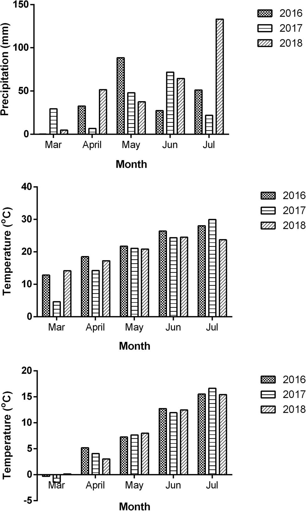
Rainfall amount, maximum and minimum temperature for the growing seasons of 2016–2018.
2.2 Experimental design and field management
This experiment is a factorial design with two factors: planting time and straw mulch. Three planting times (early, normal and late sowing times) were tested at two different straw-mulching rates (3.75 t/ha straw and 0 t/ha indicating straw-mulch and no straw-mulch respectively). This combination resulted in 3 × 2 = 6 treatments. All treatments were tilled. Thus, the six treatments tested were (1) early sowing of spring wheat without straw-mulch (ESW-T), (2) early sowing of spring wheat with straw-mulch (ESW-TS), (3) normal sowing of spring wheat without straw-mulch (NSW-T), (4) normal sowing of spring wheat with straw-mulch (NSW-TS), (5) late sowing of spring wheat without straw-mulch (LSW-T), and (6) late sowing of spring wheat with straw-mulch (LSW-TS). The treatments were replicated three times giving a total of 18 plots with each plot covering an area of 24 m2 (6 m × 4 m or 8 m × 3 m). Spring wheat (Triticum aestivum L) was used as the test crop. The Dingxi 42 genotype was used due to the prevalence of its use by farmers in the region. All plots were tilled by inverting the soil manually with shovels to a depth of 20 cm before planting. Herbicide (Red sun) with 30% glyphosate as the active ingredient was applied to control weeds in the plots before planting while manual weeding was done intermittently within the season. Wheat straw (3.75 t/ha, dry weight) was spread uniformly on all mulch-treated plots after planting. Sowing was carried out on 6th, 15th and 25th of March depicting three planting times: early sowing, normal sowing and late sowing respectively. The seeds were sown in rows with a row spacing of 25 cm. Di-ammonium phosphate (N + P2O5) was applied as basal fertilizer at a rate of 350 g/24 m2 (14.58 g/m2) and urea (46%; 18–46–0) at a rate of 150 g/24 m2 (6.25 g/m2).
2.3 Sampling and data measurements
The above-ground plant products were sampled manually at six stages including emergence, seedling, tillering, booting, maturity and final harvest stage. Three rows per plot were harvested for the determination of aboveground plant products at various growth stages while the final grain yield was obtained at physiological maturity. Biomass was determined by oven-drying plants at 80°C to constant weight [35]. At the final harvest, the wheat grain yield was separated from the final above-ground biomass, and the grain yield was determined by oven drying at 105°C for 45 min to constant weight [11]. Soil moisture content was measured at various soil depths (0–10, 10–20, 20–40 cm) with a Time Domain Reflectometry with a T3 probe connected to a hand-held meter (Aozuo Ecology Instrumentation Ltd, Beijing).
2.4 Model fitting
Biomass data at different sampling times were inputted into four non-linear models with sigmoid functions: Logistic model (equation 1), Gompertz model (equation 2), Richards model (equation 3) and Weibull model (equation 4). The models were fitted using Origin version 8.1 (OriginLab, Northampton, MA). Absolute growth rate (AGR) was calculated by taking the first derivative of the predicted biomass yield.
where Y is the biomass yield, t is the time, i.e., day of the year (DOY), Y asym is the asymptotic Y value, k is the curve steepness factor, t m is the inflection point where the growth rate becomes maximum, represented in the OriginLab as xc, while b and d are curve shape factors.
2.5 Statistical descriptors and analysis
The data from the field experiment were analyzed using SPSS version 19. Treatment effects were analyzed using one-way anova while statistical differences were separated using Duncan’s multiple-range tests at a 5% significance level. The coefficient of determination (R 2) and Root mean square error (RMSE) were employed to statistically evaluate model fitness while Akaike information criteria (AIC) was used to select the best model among the tested models. The R 2, RMSE, and AIC were calculated as shown in equations (5), (6) and (7), respectively.
The entire study process is summarized in the flowchart in Figure 2.
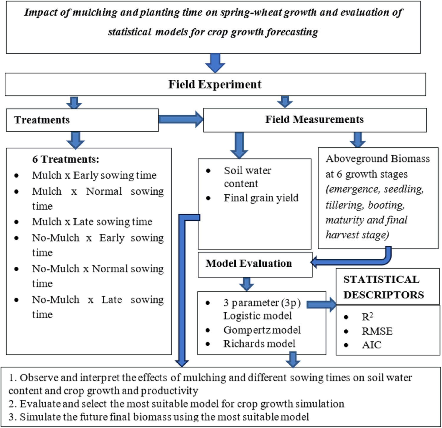
Flowchart summarizing the study methodology.
3 Results
3.1 Observed biomass accumulation over time
Observed wheat growth and its dynamics are shown in Figure 3. The growth of wheat biomass from the seedling stage (DOY 121) to the tillering stage (DOY 147) was gradual but increased rapidly between tillering and booting stages (DOY 163) and continued to maturity where growth slowed (DOY 201). The growth was sigmoid, and the growth rate decreased towards the end of the growing cycle. Comparing plots of straw-mulch with plots without straw-mulch, the growth was similar from the seedling stage to DOY 121, but there was observed higher growth under plots of straw-mulch than those without straw-mulch after DOY 147 till the maturity stage.
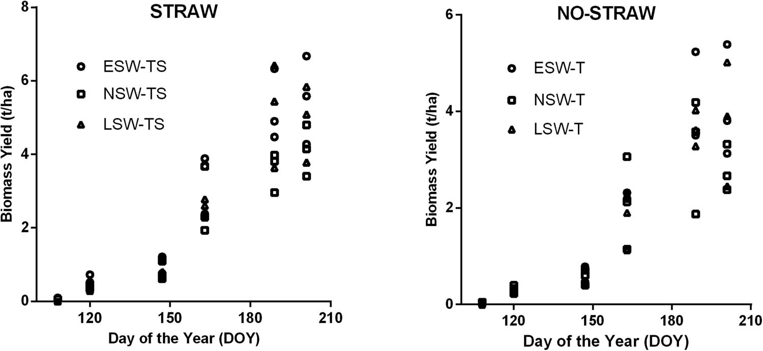
Biomass accumulation over time (straw/no straw).
3.2 Observed soil moisture content
Table 1 shows the 3-year average soil moisture content for various treatments at 0–40 cm depth. Treatments with straw-mulch, regardless of the sowing time, had higher soil moisture contents than treatments without straw-mulch. Comparing all treatments, ESW-TS and NSW-TS had significantly higher moisture contents than LSW-T and NSW-T at p < 0.05. Treatments without mulch showed soil moisture content of 10.28% ± 0.65, 9.80% ± 0.04, and 9.26% ± 0.61 times respectively for early, normal and late sowing while treatments with mulch showed moisture content of 10.93% ± 0.51, 10.88% ± 0.29 and 10.33% ± 0.15, respectively, for early, normal and late sowing. This showed that early sowing improved water storage compared with the normal and late sowing times.
Soil water content under mulch treatment at different planting times
| Treatment | S WC (0–40 cm) (%) |
|---|---|
| ESW-T | 10.28 ± 0.65ab |
| ESW-TS | 10.93 ± 0.51a |
| NSW-T | 9.80 ± 0.04b |
| NSW-TS | 10.88 ± 0.29a |
| LSW-T | 9.26 ± 0.61c |
| LSW-TS | 10.33 ± 0.15ab |
(a–c) Treatments with uncommon letters are statistically different at p ≤ 0.05.
3.3 Observed final biomass yield
The average final biomass analysis showed that planting time, straw-mulching and their interactions influenced biomass growth significantly (Table 2). Generally, at maturity, higher biomass was obtained under mulch treatments compared with no-mulch treatments while early planting also resulted in increased biomass yield. All mulch treatments showed significantly higher (p < 0.05) final biomass yields under all sowing times except late sowing which was also higher but not significantly different (Table 3). Mulch-straw amendments increased biomass by 14.5% and 17.4% at early and normal planting times, respectively, compared to their corresponding no-mulch treatments. On average, planting early resulted in higher biomass than normal and late planting (Table 4). The combination of early planting with straw-mulch (ESW-TS) resulted in the highest final biomass, while normal planting time without straw-mulch (NSW-T) gave the lowest final biomass. Using NSW-T as a control, biomass yield in ESW-TS was 37.9% greater and significantly higher (p < 0.05) than NSW-T (Table 3).
ANOVA table of treatment effects and interaction
| Source | Type III sum of squares | df | Mean square | F | Sig. |
|---|---|---|---|---|---|
| Corrected model | 3958404.436a | 5 | 791680.887 | 126.128 | 0.000 |
| Intercept | 328812496.82 | 1 | 328812496.82 | 52385.495 | 0.000 |
| Sowing time | 2686966.363 | 2 | 1343483.181 | 214.040 | 0.000 |
| Mulch | 827618.317 | 1 | 827618.317 | 131.854 | 0.000 |
| Sowing time × Mulch | 443819.757 | 2 | 221909.878 | 35.354 | 0.000 |
| Error | 75321.422 | 12 | 6276.785 | ||
| Total | 332846222.678 | 18 | |||
| Corrected total | 4033725.858 | 17 |
a R Squared = 0.981 (adjusted R squared = 0.974).
Effect of mulching on biomass yield
| Sowing time | Total biomass (kg/ha) | |
|---|---|---|
| Mulch | No-Mulch | |
| Early sowing time | 5143.41 ± 181.74a | 4490.61 ± 10.34b |
| Normal sowing time | 4379.94 ± 26.13b | 3730.91 ± 15.61d |
| Late sowing time | 3942.03 ± 37.01c | 3957.29 ± 47.20c |
(a–d) Treatments with uncommon letters are statistically different at p ≤ 0.05.
Planting time effects on biomass yield
| Planting time | Total biomass yield (kg/ha) |
|---|---|
| Early | 4817.01 ± 375.63a |
| Normal | 4055.42 ± 356.01b |
| Late | 3949.67 ± 38.84c |
(a–c) Treatments with uncommon letters are statistically different at p ≤ 0.05.
3.4 Evaluation of model suitability
3.4.1 Model convergence
As indicated by Pinheiro and Bates [36], choosing informed starting estimates for parameters can facilitate model convergence. In this study, Figure 3 was used as a guide in choosing starting values of model parameters. Estimates and standard errors of model parameters were obtained (Table 5), and model convergence was achieved for all models (Logistic, Gompertz and Weibull models) except the Richards model. Parameter estimates showed low standard errors for the three models indicating good algorithm convergence and suitability of the models in describing our data. The Richards model however showed extremely large standard errors for the parameters estimated in five out of the six treatments (Table 5).
Parameter estimates for four non-linear regression models for 6 treatments at different planting times
| Model | Parameter | Parameter estimate | |||||
|---|---|---|---|---|---|---|---|
| ESW-T | ESW-TS | NSW-T | NSW-TS | LSW-T | LSW-TS | ||
| 3p logistic | Ym | 4.51 ± 0.47 | 5.56 ± 0.38 | 3.01 ± 0.27 | 3.95 ± 0.26 | 3.97 ± 0.45 | 5.16 ± 0.37 |
| xc | 164.73 ± 5.17 | 159.78 ± 3.08 | 156.98 ± 3.61 | 157.70 ± 2.94 | 165.25 ± 5.12 | 162.76 ± 3.06 | |
| k | 0.08 ± 0.03 | 0.10 ± 0.03 | 0.14 ± 0.06 | 0.11 ± 0.03 | 0.09 ± 0.04 | 0.12 ± 0.04 | |
| Gompertz | Ym | 4.48 ± 0.49 | 5.71 ± 0.51 | 3.03 ± 0.30 | 4.03 ± 0.33 | 4.26 ± 0.74 | 5.42 ± 0.59 |
| xc | 157.01 ± 3.24 | 154.49 ± 2.75 | 152.31 ± 3.36 | 152.76 ± 2.60 | 160.03 ± 5.03 | 157.82 ± 3.22 | |
| k | 0.07 ± 0.03 | 0.07 ± 0.02 | 0.10 ± 0.04 | 0.08 ± 0.03 | 0.06 ± 0.03 | 0.07 ± 0.03 | |
| Richards | Ym | 4.21 ± 0.26 | 5.37 ± 0.29 | 3.00 ± 0.26 | 3.85 ± 0.22 | 3.80 ± 0.45 | 5.04 ± 0.28 |
| xc | 170.10 ± 1.17 × 10⁶ | 168.78 ± 4.10 × 10⁵ | 166.42 ± 4.12 × 10⁵ | 167.23 ± 3.66 × 10⁵ | 168.51 ± 8.76 | 170.36 ± 9.95 × 10⁵ | |
| d | 20.79 ± 1.60 × 10⁷ | 25.01 ± 6.81 × 10⁶ | 31.95 ± 1.18 × 10⁷ | 31.01 ± 8.89 × 10⁶ | 3.50 ± 5.29 | 19.35 ± 1.25 × 10⁷ | |
| k | 1.37 ± 1.10 × 10⁶ | 1.51 ± 4.28 × 10⁵ | 2.25 ± 8.55 × 10⁵ | 1.95 ± 5.77 × 10⁵ | 0.16 ± 0.27 | 8.89 × 10⁵ | |
| Weibull | Ym | 4.5 ± 0.00 | 5.37 ± 0.28 | 3.00 ± 0.26 | 3.85 ± 0.22 | 3.75 ± 0.28 | 5.04 ± 0.28 |
| b | 0.13 ± 0.262 | 0.30 ± 0.30 | 0.17 ± 0.27 | 0.22 ± 0.23 | 0.12 ± 0.26 | 0.14 ± 0.30 | |
| d | 15.06 ± 7.74 | 16.56 ± 6.84 | 19.43 ± 11.53 | 17.36 ± 6.74 | 13.25 ± 7.30 | 15.70 ± 8.19 | |
| k | 0.006 ± 1.35 × 10⁻⁴ | 0.006 ± 9.26 × 10⁻⁵ | 0.006 ± 1.26 × 10⁻⁴ | 0.006 ± 9.10 × 10⁻⁵ | 0.006 ± 2.04 × 10⁻⁴ | 0.006 ± 1.32 × 10⁻⁴ | |
3.4.2 Robustness of the candidate models and model selection
In order to have confidence in the prediction of the models tested, model assumptions have to meet some criteria. A good model should have errors that are normally distributed, and independent and should have homogeneous variance [22]. This can be done by observing the residual plots for patterns. In this experiment, a plot of residuals against fitted values showed no clear pattern for all the models and ranged between −1.5 and 1.5 (Figure 4), indicating independence of errors, normal distribution and homogeneity in variance.
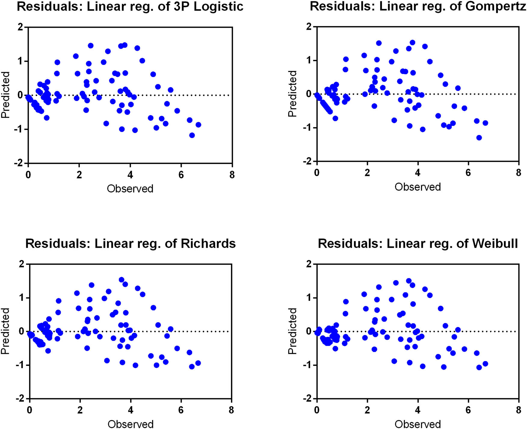
Plot of residuals against fitted values.
All four models (Logistic, Gompertz, Richards and Weibull models) predicted biomass close to the observed, especially for final biomass (Figure 5). However, due to large standard errors of parameter estimates in the Richards model, it may not be suitable for describing the growth data in this study. All models under-predicted biomass at the seedling stage but the Gompertz model was worse in predicting biomass at this stage. With all treatments put together, plots of predicted biomass against measured biomass showed a high correlation for all the models with R 2 values of 0.9148, 0.9125, 0.9153 and 0.9148, respectively, for the 3p-Logistic, Gompertz, Richards and Weibull models (Figure 5). All the regression slopes were also close to 1 while the intercepts were close to 0 (Figure 5). The R 2 value and RMSE were used to further evaluate the goodness of fit of the models while AIC was used to select the overall best model (Table 6). On the basis of the R 2 value, the Logistic model had the highest value for almost all the treatments while the Gompertz model was next by being higher than the other two models in four out of six treatments.
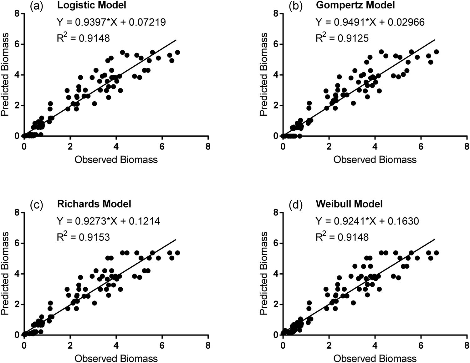
Linear regression plot of predicted biomass against measured biomass. (a–d) Treatments with uncommon letters are statistically different at p ≤ 0.05.
Statistical descriptors for model evaluation
| Treatment | 3p-Logistic model | Gompertz model | Richards model | Weibull model | ||||||||
|---|---|---|---|---|---|---|---|---|---|---|---|---|
| Statistical descriptor | ||||||||||||
| R 2 | ∆AIC | RMSE | R 2 | ∆AIC | RMSE | R 2 | ∆AIC | RMSE | R 2 | ∆AIC | RMSE | |
| ESW-T | 0.902 | 0.00 | 0.499 | 0.897 | 0.78 | 0.535 | 0.899 | 3.37 | 0.512 | 0.898 | 0.65 | 0.533 |
| ESW-TS | 0.914 | 0.00 | 0.626 | 0.912 | 0.51 | 0.635 | 0.911 | 3.36 | 0.616 | 0.912 | 3.03 | 0.610 |
| NSW-T | 0.802 | 0.00 | 0.569 | 0.799 | 0.23 | 0.573 | 0.792 | 3.49 | 0.562 | 0.795 | 3.28 | 0.559 |
| NSW-TS | 0.903 | 0.00 | 0.480 | 0.902 | 0.10 | 0.482 | 0.898 | 3.52 | 0.475 | 0.900 | 3.24 | 0.471 |
| LSW-T | 0.890 | 0.00 | 0.505 | 0.886 | 0.59 | 0.513 | 0.883 | 3.67 | 0.502 | 0.884 | 3.64 | 0.501 |
| LSW-TS | 0.910 | 0.00 | 0.616 | 0.905 | 0.96 | 0.633 | 0.908 | 3.13 | 0.603 | 0.908 | 3.12 | 0.603 |
| Average | 0.887 | 0.0 | 0.549 | 0.884 | 0.53 | 0.562 | 0.882 | 3.42 | 0.545 | 0.883 | 2.83 | 0.546 |
3.5 Model simulations
The model fit for all six treatments is shown in Figure 6. The logistic model across the six treatments estimated wheat biomass perfectly which reached a maximum of 5.5 Mg/ha under ESW-TS (Figure 6b). The simulated maximum biomass followed the order: ESW-TS > LSW-TS > ESW-T > NSW-TS > LSW-T > NSW-T. The simulated maximum biomass in ESW-TS (Figure 6b) was 45% higher than the maximum biomass simulated under NSW-T (Figure 6c), which was the least. NSW-T and NSW-TS reached the upper horizontal asymptote before DOY 180 (Figure 6c and d), meanwhile those of ESW-T, ESW-TS, LSW-T and LSW-TS occurred after DOY 180 (Figure 6a,b,e,f).
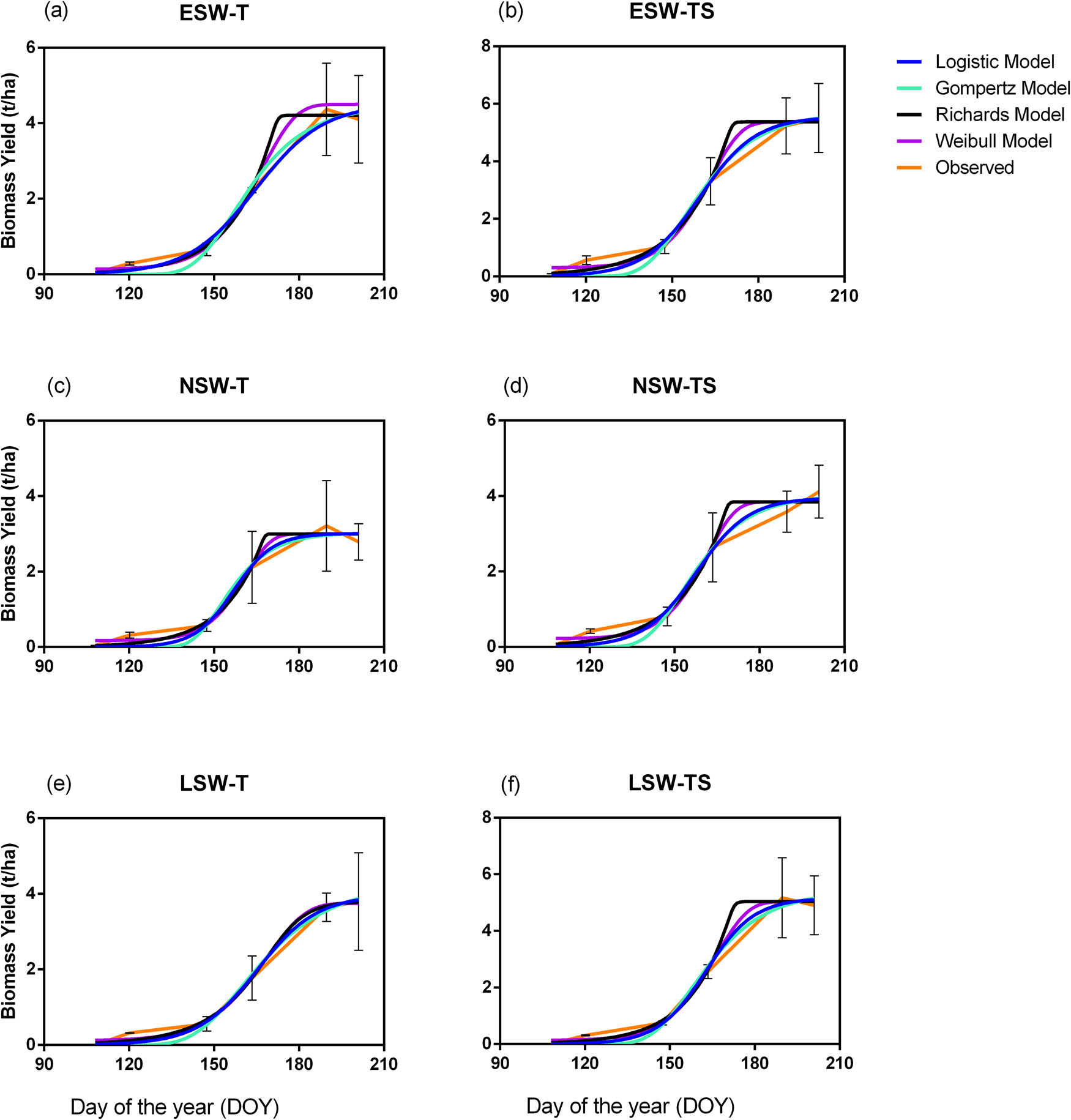
Fitting of biomass yields with four non-linear models under straw and no-straw treatments. (a–f) Treatments with uncommon letters are statistically different at p ≤ 0.05.
Using the logistic model again for absolute growth rate (AGR) analysis, peak AGR was found in LSW-TS (Figure 7). Under early sowing time, ESW-TS showed peak AGR at DOY 160 which occurred 3 days earlier and was 13% higher in magnitude than that of ESW-T while with late sowing, LSW-TS was 38% higher in magnitude and preceded that of LSW-T by 2 days. Contrastingly, with normal sowing time, peak AGR in NSW-T was 1% higher in magnitude than the straw-mulch treatment (NSW-TS) and preceded it by 1 day.
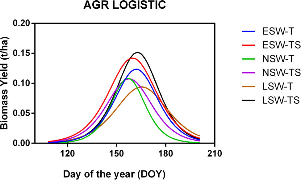
AGR curves for four non-linear models under straw and non-straw treatments at different planting time.
3.6 Discussion of Impact of straw-mulch and early planting on soil moisture and biomass growth
Crop growth followed a sigmoid pattern by growing gradually, followed by a steep growth and finally reduced slightly towards the end of the season. This growth pattern can be explained by a number of factors: (1) growth rate may decrease at the tail-end as a result of accumulation of non-photosynthetic dry matter as roots and stems, (2) self-shading of leaves may also reduce the capture of sunlight for photosynthesis in the shaded leaves and (3) decreases in nutrient concentrations over time may limit biomass growth [20].
Relatively higher water retention in mulched plots is similar to the results of a study by Zhao et al. [37] where mulched plots showed an increase in soil moisture. This is also supported by Akhtar et al. [38] who indicated that soil hydrothermal conditions improved after mulch treatments and provided favorable conditions for crop growth. The increase in soil moisture could be a result of a reduction in evapotranspiration, as straw-mulch may have acted as a cover over the soil, thereby slowing down the transport of water out of the soil medium. Straw-mulch could also prevent the direct impact of raindrops, which could prolong the stay of rainwater on the field and provide enough time for infiltration [39]. Furthermore, the release of carbon into the soil from the mulch straw may have also occurred, resulting in improved soil structure and increased infiltration. This assertion is supported by other researchers. For instance, Liu et al [7] reported increased water storage in straw-mulched plots due to the effective retention of precipitation. In another study, Zhu et al. [40] expounded that maize straw-mulch amendment influenced significantly the release of dissolved organic carbon and easily oxidizable carbon into soils within 35 days after straw application.
The higher yield obtained under early sowing may have been due to early utilization of rainfall by crops while the addition of straw-mulch may have caused improvement in soil physical and chemical properties. Improved soil hydrothermal conditions may have also enhanced nutrient uptake and allocation for dry matter production. Some studies in other parts of China have shown the influence of planting time on wheat yield [41]. The study of Xiao et al. [42] also showed that early planting increased spring-wheat yield even though under irrigation. This could be due to the influence of planting time on crop growth stages and also aligning of the crop growth process to weather conditions [43,44].
3.7 Discussion of model evaluation and simulation
Large standard errors during model convergence tests are indications of non-convergence of the model [22]. A non-converging model may not be useful for describing the data and is not suitable for future predictions. The Richards model, showed very large standard errors as shown in Table 5, thus not suitable for predictions of future crop cultivation alternatives in this study area,. Hence the Richard model was rejected at this stage.
Other model evaluation procedures as indicated in the results showed that the logistic model was better on the basis of R 2 and AIC. The logistic model with the highest R 2 value is indicative of its higher correlation and very high percentage of fitness of the data in the model. The AIC value is a criterion for comparison among models in order to select the best among the lot. The model with the least change in AIC (∆AIC) score compared with the other models shows that among the candidate models, it is the best in describing the data. In this study, the logistic model showed the lowest ∆AIC when compared with the rest, hence most suitable for prediction. In addition, on the basis of RMSE, the model with a smaller RMSE value also shows better performance than that with a higher RMSE value. On this basis, the logistic model was still better than the Gompertz model but could not outperform the Richards and Weibull models. However, the Richards model was already rejected earlier due to large standard errors of estimates. The Richards model again had the highest values of ∆AIC reiterating its poor performance among the candidate models. Based on all these statistics, the logistic model was the best for simulating wheat biomass accumulation under the treatments in this study. The models may therefore be arranged according to their performance as follows: Logistic > Gompertz > Weibull > Richards. According to Ahmed et al. [45], a model that simulates biomass accurately is robust and could be used in making crop management decisions since biomass has a strong relation with grain yield.
There were lower yields recorded and predicted in this study compared to other studies elsewhere. A study in Pakistan by Ahmed et al. [45] predicted a yield of 7.63–13.21 t/ha while a similar study by Zhang et al. [1] on the Loess Plateau predicted maximum biomass of above 12.0 t/ha. The low yields in our experiment could be attributed to the generally lower precipitation and poor soil fertility in our study area. Under NSW-T and NSW-TS, the biomass growth reached the upper horizontal asymptote before DOY 180 (Figure 6c and d), which shows that the growth period was shortened possibly due to lower moisture availability and or poor nutrient uptake. However, early planting and stubble mulch as in ESW-TS played a significant role in crop growth in this study, eventually enhancing yield under ESW-TS. As indicated from the model simulations, ESW-TS treatment gave the highest biomass compared to other treatments. This is an indication that early planting combined with mulching could lead to maximization of the use of available rainwater to achieve maximum yield. This means that adopting ESW-TS could ameliorate the effect of climate change, soil degradation and poor soil fertility in this study area. This should be encouraged in the semi-arid western Loess Plateau and similar dry land areas. Higher crop productivity also has a beneficial role in sustaining the environment as a whole and mitigating climate change. As indicated by Yeboah et al. [11], higher productivity often results in higher net primary production and holds a huge potential of soil carbon sequestration [46].
4 Conclusion and recommendations
This study assessed the impact of mulching and sowing time on spring-wheat growth and evaluated the performance of nonlinear regression models in describing and forecasting spring-wheat growth. Comparing mulch and no-mulch treatments, mulch treatments improved soil water retention and supported higher biomass growth. There was also an interaction between mulching and sowing time. Mulched treatments significantly increased biomass yield when planting was done early. Biomass yield almost doubled in ESW-TS when compared with the normal sowing time and the farmers’ practice of not mulching (NSW-T).
The logistic model best-described crop growth, based on AIC and R 2 values. Simulation results with the logistic model showed that the highest biomass yield was also obtained under ESW-TS. The logistic model is recommended for forecasting crop response to soil conservation technologies in the dryland areas of Northwestern China. This would be useful for crop management planning in response to climate change for sustainable crop production. Furthermore, early sowing and straw-mulching is recommended for the improvement of wheat yields in the dry-land areas, particularly on the Northwestern Loess Plateau of China. These results also indicate that nonlinear regression models, when properly calibrated could be valuable tools for quick and accurate decision-making in farm management. Further research may be required for the comparative evaluation of descriptive models and process models for crop growth simulation on the Loess Plateau.
Acknowledgments
I wish to acknowledge the invaluable advice and guidance given to me by Dr Guopeng Chen during the experiment.
-
Funding information: The author states no funding involved.
-
Conflict of interest: The author states no conflict of interest.
-
Data availability statement: The datasets generated during and/or analyzed during this study are available at 10.6084/m9.figshare.19387520.
References
[1] Zhang W, Liu W, Xue Q, Chen J, Han X. Evaluation of the AquaCrop model for simulating yield response of winter wheat to water on the southern Loess Plateau of China. Water Sci Technol. 2013;68(4):821–8. 10.2166/wst.2013.305.Search in Google Scholar PubMed
[2] Ye L, Xiong W, Li Z, Yang P, Wu W, Yang G, et al. Climate change impact on China food security in 2050. Agron Sustain Dev. 2013;33(2):363–74. 10.1007/s13593-012-0102-0.Search in Google Scholar
[3] Gan YT, Campbell CA, Liu L, Basnyat P, McDonald CL. Water use and distribution profile under pulse and oilseed crops in semi-arid northern high latitude areas. Agric Water Manag. 2009;96(2):337–48. 10.1016/j.agwat.2008.08.012.Search in Google Scholar
[4] Jabal ZK, Khayyun TS, Alwan IA. Impact of climate change on crops productivity using MODIS-NDVI time series. Civ Eng J. 2022;8(6):1136–56. 10.28991/cej-2022-08-06-04.Search in Google Scholar
[5] Chen H, Hou R, Gong Y, Li H, Fan M, Kuzyakov Y. Effects of 11 years of conservation tillage on soil organic matter fractions in wheat monoculture in Loess Plateau of China. Soil Tillage Res. 2009;106(1):85–94. 10.1016/j.still.2009.09.009.Search in Google Scholar
[6] Huang GB, Luo ZZ, Li LL, Zhang RZ, Li GD, Cai LQ, et al. Effects of stubble management on soil fertility and crop yield of rainfed area in Western Loess Plateau, China. Appl Environ Soil Sci. 2012;2012(1–9). 10.1155/2012/256312.Search in Google Scholar
[7] Liu XE, Li XG, Hai L, Wang YP, Li FM. How efficient is film fully-mulched ridge–furrow cropping to conserve rainfall in soil at a rainfed site? Field Crops Res. 2014;169:107–15. 10.1016/j.fcr.2014.09.014.Search in Google Scholar
[8] Līcīte I, Popluga D, Rivža P, Lazdiņš A, Meļņiks R. Nutrient-rich organic soil management patterns in light of climate change policy. Civ Eng J. 2022;8(10):2290–304. 10.28991/cej-2022-08-10-017.Search in Google Scholar
[9] White PJ, Crawford JW, Díaz Álvarez MC, García Moreno R. Soil management for sustainable agriculture. Appl Environ Soil Sci. 2012;2012:1–3. 10.1155/2012/850739.Search in Google Scholar
[10] Zhang S, Lövdahl L, Grip H, Tong Y, Yang X, Wang Q. Effects of mulching and catch cropping on soil temperature, soil moisture and wheat yield on the Loess Plateau of China. Soil Tillage Res. 2009;102:78–86. 10.1016/j.still.2008.07.019.Search in Google Scholar
[11] Yeboah S, Zhang RZ, Cai LQ, Li LL, Xie JH, Luo ZZ, et al. Tillage effect on soil organic carbon, microbial biomass carbon and crop yield in spring wheat-field pea rotation. Plant Soil Environ. 2016;62:279–85. 10.17221/66/2016-PSE.Search in Google Scholar
[12] Lamptey S, Li LL, Xie JH, Zhang RZ, Luo ZZ, Cai LQ, et al. Soil respiration and net ecosystem production under different tillage practices in semi-arid Northwest China. Plant Soil Environ. 2017;63:14–21. 10.17221/403/2016-PSE.Search in Google Scholar
[13] Liu XE, Li XG, Hai L, Wang YP, Fu TT, Turner NC, et al. Film-mulched ridge–furrow management increases maize productivity and sustains soil organic carbon in a dryland cropping system. Soil Sci Soc Am J. 2014;78:1434–41. 10.2136/sssaj2014.04.0121.Search in Google Scholar
[14] Araya A, Kisekka I, Gowda PH, Prasad PV. Evaluation of water-limited cropping systems in a semi-arid climate using DSSAT-CSM. Agric Syst. 2017;150:86–98. 10.1016/j.agsy.2016.10.007.Search in Google Scholar
[15] Brown H, Huth N, Holzworth D. Crop model improvement in APSIM: using wheat as a case study. Eur J Agron. 2018;100:141–50. 10.1016/j.eja.2018.02.002.Search in Google Scholar
[16] Rajak AA. Emerging technological methods for effective farming by cloud computing and IoT. Emerg Sci J. 2022;6(5):1017–31. 10.28991/esj-2022-06-05-07.Search in Google Scholar
[17] Kumar A, Kumar A, Singh AK, Choudhary AK. IoT based energy efficient agriculture field monitoring and smart irrigation system using NodeMCU. J Mob Multimed. 2021;17(1–3):345–60. 10.13052/jmm1550-4646.171318.Search in Google Scholar
[18] Rabhi L, Falih N, Afraites L, Bouikhalene B. A functional framework based on big data analytics for smart farming. Indones J Electr Eng Comp Sci. 2021;24(3):1772–9. 10.11591/ijeecs.v24.i3.pp1772-1779.Search in Google Scholar
[19] Fontes L, Bontemps JD, Bugmann H, Van Oijen M, Gracia C, Kramer K, et al. Models for supporting forest management in a changing environment. For Syst. 2010;19:8–29. 10.5424/fs/201019s-9315.Search in Google Scholar
[20] Paine CE, Marthews TR, Vogt DR, Purves D, Rees M, Htor A, et al. How to fit nonlinear plant growth models and calculate growth rates: an update for ecologists. Methods Ecol Evol. 2012;3(2):245–56. 10.1111/j.2041-210X.2011.00155.x.Search in Google Scholar
[21] Teh C. Introduction to mathematical modeling of crop growth: How the equations are derived and assembled into a computer model. Dissertation. com. Boca Raton, Florida, USA: Brown Walker Press; 2006. ISBN:1-58-112-998-X.Search in Google Scholar
[22] Archontoulis SV, Miguez FE. Nonlinear regression models and applications in agricultural research. Agron J. 2015;107:786–98. 10.2134/agronj2012.0506.Search in Google Scholar
[23] Yin X, Goudriaan JAN, Lantinga EA, Vos JAN, Spiertz HJ. A flexible sigmoid function of determinate growth. Ann Bot. 2003;91:361–71. 10.1093/aob/mcg029.Search in Google Scholar PubMed PubMed Central
[24] Shafii B, Price WJ, Swensen JB, Murray GA. Nonlinear estimation of growth curve models for germination data analysis. Annual Conference on Applied Statistics in Agriculture; 1991. http://newprairiepress.org/agstatconference/1991/proceedings/3.10.4148/2475-7772.1415Search in Google Scholar
[25] Yin X, Kropff MJ, McLaren G, Visperas RM. A nonlinear model for crop development as a function of temperature. Agric For Meteorol. 1995;77:1–16. 10.1016/0168-1923(95)02236-Q.Search in Google Scholar
[26] Birnbaum A. Some latent trait models and their use in inferring an examinee’s ability. In: Lord FM, Novick MR, editors. Statistical Theories of Mental Test Scores. Reading, MA: Addison-Wesley; 1968. p. 17–20.Search in Google Scholar
[27] Rymuza K, Bombik A. Application of a logistic function to describe the growth of Fodder Galega. J Ecol Eng. 2017;18(1):125–31. 10.12911/22998993/66245.Search in Google Scholar
[28] Weibull W. A statistical distribution function of wide applicability. J Appl Mech. 1951;18(3):293–7. 10.1115/1.4010337.Search in Google Scholar
[29] Reynolds WD, Drury CF, Phillips LA, Yang X, Agomoh IV. An adapted Weibull function for agricultural applications. Can J Soil Sci 101(4):680–702. 10.1139/cjss-2021-0046.Search in Google Scholar
[30] Richards FJ. A flexible growth function for empirical use. J Exp Bot. 1959;10(2):290–301. 10.1093/jxb/10.2.290.Search in Google Scholar
[31] Hsieh YH. Richards model: a simple procedure for real-time prediction of outbreak severity. In: Modeling and Dynamics of Infectious Diseases. Higher Education Press; 2009. p. 216–36.10.1142/9789814261265_0009Search in Google Scholar
[32] Tjørve KMC, Tjørve E. The use of Gompertz models in growth analyses, and new Gompertz-model approach: An addition to the Unified-Richards family. Plos One. 2017;12(6):e0178691. 10.1371/journal.pone.0178691.Search in Google Scholar PubMed PubMed Central
[33] Aggrey SE. Comparison of three nonlinear and spline regression models for describing chicken growth curves. Poult Sci. 2002;81:1782–8. 10.1093/ps/81.12.1782.Search in Google Scholar PubMed
[34] Benzekry S, Lamont C, Beheshti A, Tracz A, Ebos JM, Hlatky L, et al. Classical mathematical models for description and prediction of experimental tumor growth. PLoS Comput Biol. 2014;10(8):e1003800. 10.1371/journal.pcbi.1003800.Search in Google Scholar PubMed PubMed Central
[35] Alhassan ARM, Ma W, Li G, Jiang Z, Wu J, Chen G. Response of soil organic carbon to vegetation degradation along a moisture gradient in a wet meadow on the Qinghai–Tibet Plateau. Ecol Evol. 2018;8(23):11999–2010. 10.1002/ece3.4656.Search in Google Scholar PubMed PubMed Central
[36] Pinheiro J, Bates D. Mixed-Effects Models in S and S-PLUS. New York: Springer Verlag; 2000.10.1007/978-1-4419-0318-1Search in Google Scholar
[37] Zhao Y, Pang H, Wang J, Huo L, Li Y. Effects of straw mulch and buried straw on soil moisture and salinity in relation to sunflower growth and yield. Field Crops Res. 2014;161:16–25. 10.1016/j.fcr.2014.02.006.Search in Google Scholar
[38] Akhtar K, Wang W, Khan A, Ren G, Afridi MZ, Feng Y, et al. Wheat straw mulching offset soil moisture deficient for improving physiological and growth performance of summer sown soybean. Agric Water Manag. 2019;211:16–25. 10.1016/j.agwat.2018.09.031.Search in Google Scholar
[39] Bhatt R, Khera KL. Effect of tillage and mode of straw mulch application on soil erosion in the submontaneous tract of Punjab, India. Soil Tillage Res. 2006;88(1–2):107–15. 10.1016/j.still.2005.05.004.Search in Google Scholar
[40] Zhu LX, Xiao Q, Shen YF, Li SQ. Effects of biochar and maize straw on the short-term carbon and nitrogen dynamics in a cultivated silty loam in China. Environ Sci Poll Res. 2017;24:1019–29. 10.1007/s11356-016-7829-0.Search in Google Scholar PubMed
[41] Sun H, Zhang X, Chen S, Pei D, Liu C. Effects of harvest and sowing time on the performance of the rotation of winter wheat–summer maize in the North China Plain. Ind Crops Prod. 2007;25(3):239–47. 10.1016/j.indcrop.2006.12.003.Search in Google Scholar
[42] Xiao D, Cao J, Bai H, Qi Y, Shen Y. Assessing the impacts of climate variables and sowing date on spring wheat yield in the Northern China. Int J Agric Biol. 2017;19:1551–8.Search in Google Scholar
[43] Zia-ul-hassan M, Wahla AJ, Waqar MQ, Ali A. Influence of sowing date on the growth and grain yield performance of wheat varieties under rainfed condition. Sci Technol Dev. 2014;33(1):22‒5.Search in Google Scholar
[44] Xiao D, Tao F. Contributions of cultivar shift, management practice and climate change to maize yield in North China Plain in 1981‒2009. Int J Biometeorol. 2016;60(7):1111–22. 10.1007/s00484-015-1104-9.Search in Google Scholar PubMed
[45] Ahmed M, Akram MN, Asim M, Aslam M, Hassan FU, Higgins S, et al. Calibration and validation of apsim-wheat and ceres-wheat for spring wheat under rainfed conditions: models evaluation and application. Comput Electron Agric. 2016;123(C):384–401. 10.1016/j.compag.2016.03.015.Search in Google Scholar
[46] Lamptey S, Li LL, Xie JH. Impact of nitrogen fertilization on soil respiration and net ecosystem production in maize. Plant Soil Environ. 2018;64:353–60. 10.17221/217/2018-PSE.Search in Google Scholar
© 2024 the author(s), published by De Gruyter
This work is licensed under the Creative Commons Attribution 4.0 International License.