Dimension Independent Data Sets Approximation and Applications to Classification

Abstract.

We revisit the classical kernel method of approximation/interpolation theory in a very specific context motivated by the desire to obtain a robust procedure to approximate discrete data sets by (super)level sets of functions that are merely continuous at the data set arguments but are otherwise smooth. Special functions, called data signals, are defined for any given data set and are used to succesfully solve supervised classification problems in a robust way that depends continuously on the data set. The efficacy of the method is illustrated with a series of low dimensional examples and by its application to the standard benchmark high dimensional problem of MNIST digit classification.

1. Introduction

The problem of finding a function that explains a given set of data is a fundamental problem in mathematics and statistics. If the data are assumed to be the discrete manifestation of a function defined on a continuous (as opposed to discrete) domain of definition, the problem can be viewed as an approximation problem where the data can be leveraged to help identify a sensible approximation to the function. Often one resorts the prior knowledge about the target function to reduce the set of candidates from which to choose a good approximation, if not the best approximation. Within this framework, an extensive mathematical knowledge has been obtained over the past several decades along with a variety of powerful tools (see [5], in particular, for the philosophical approach taken here). In the current world, where data about almost anything you can imagine or wish for is available, one of the most interesting and often challening problems consists in extracting information, knowledge, and structure from high dimensional data. A variety of commonly used approaches belong to a category referred to as Machine Learning. Neural networks in all forms and shapes are particularly widespread due to their success in dealing with a series of challenging problems. Another class is that of Support-Vector Machines (SVM) [4], which were very popular before being somewhat superseded by improved neural networks . While they often use linear classification via hyperlanes, the so-called kernel trick [1, 2] makes it possible for them to capture nonlinear decision boundaries albeit at the cost of working in a higher dimensional space to which the data is mapped but that admits an efficient computation of scalar products (via a suitable kernel). A connection between SVMs and neural networks was discovered in [3] and has since been investigated by many more authors. The method proposed here is philosophically in the category of SVMs but distinguishes itself by directly working with the data at hand without embedding into a higher dimensional feature space. We first review a classical method of inexact interpolation that yields a continuous function approximating a given data set. We do so by taking a PDE perspective that reveals important features that are exploited in order to obtain the announced stable method of classification even when the distribution of available data is not uniform in space and, possibly, noisy. In high dimension, even large data sets are often sparse due to the so-called curse of dimensionality. Moreover, the data is often supported on lower dimensional manifolds, where even dense data make up a thin slice of the ambient space. In the latter case, it is demonstrated in this paper that, while the data may not be sufficient for the reliable identification of a well-defined global approximant, it can still be used fruitfully (in a global or local fashion) for data analysis purposes. This is mainly due to the fact that the proposed method is capable of connecting the dots (data points) into a manifold by capturing geometric features of the data.

It is widely understood and accepted that a function interpolating discrete data should be at least continuous so as to provide a certain stability of prediction and resilience in the face of noise. In learning problems this is sometimes expressed as local constancy, even if that does not require continuity. Unless the data is known to stem from a very smooth underlying function, but, typically, even in that case, it should also not be exceedingly smooth, as this would lead to some blurring and reduce its ability to capture sharp transitions. It would, moreover, be advantageous for the interpolating function to depend at least continuously on the data set it is constructed from. This would make it robust with respect to data uncertainty and thus defensible, for example, against what in the learning community would be referred to as adversarial attacks. These in fact use the very sensititve dependence of the model parameters on the training set.

The starting point is a set of data consisting of point/value pairs

$$\mathbb{D}=\big{\{}(x^{i},y^{i})\,\big{|}\,i=1,\dots,m\big{\}}$$

where $m\in\mathbb{N}$, $x^{i}\in\mathbb{R}^{d}$ and $y^{i}\in\mathbb{R}^{n}$, $i=1,\dots,m$, for $d,n\in\mathbb{N}$. In order to enforce minimal regularity on the interpolant function

$$u:\mathbb{R}^{d}\to\mathbb{R}^{n}$$

we take it from the space

$$\operatorname{H}^{\frac{d+1}{2}}(\mathbb{R}^{d},\mathbb{R}^{n})=\big{\{}u\in\mathcal{S}^{\prime}\,\big{|}\,[\xi\mapsto(1+|\xi|^{2})^{\frac{d+1}{2}}\hat{u}(\xi)]\in\operatorname{L}^{2}(\mathbb{R}^{d},\mathbb{R}^{n})\big{\}}.$$

Thanks to the general Sobolev inequality it holds that

$$\operatorname{H}^{\frac{d+1}{2}}(\mathbb{R}^{d},\mathbb{R}^{n})\hookrightarrow\operatorname{BUC}^{\frac{1}{2}}(\mathbb{R}^{d},\mathbb{R}^{n}),$$ (1.1)

where the containing space is that of bounded and uniformly Hölder continuous functions of exponent $\frac{1}{2}$. In order to obtain stability we may sacrifice some interpolation accuracy by not necessarily requiring the exact validity of

$$u(x^{i})=y^{i}\text{ for }i=1,\dots,m.$$ (1.2)

Then, for approximate interpolation, $u$ is determined by minimization of the energy functional given by

$$E_{\alpha}(u) =\frac{\alpha}{2c_{d}}\int_{\mathbb{R}^{d}}\big{|}(1-\Delta)^{\frac{d+1}{4}}u(x)\big{|}^{2}\,dx+\frac{1}{2}\sum_{i=1}^{m}\big{|}u(x^{i})-y^{i}\big{|}^{2}$$ (1.3)

$$=\frac{\alpha}{2c_{d}}\|u\|_{\operatorname{H}^{\frac{d+1}{2}}}^{2}+\frac{1}{2}\sum_{i=1}^{m}\big{|}u(x^{i})-y^{i}\big{|}^{2},\>u\in\operatorname{H}^{\frac{d+1}{2}}(\mathbb{R}^{d},\mathbb{R}^{n})$$ (1.4)

for $\alpha>0$ and where the normalizing constant $c_{d}$ will be explicitly given in the next section. For exact interpolation $u$ is determined by minimization of $E_{0}=\|\cdot\|_{\operatorname{H}^{\frac{d+1}{2}}}^{2}$ with constraints (1.2) that shall be summarized as $u(\mathbb{X})=\mathbb{Y}$. Formally, it is set

$$u_{\mathbb{D},\alpha}=\begin{cases}\operatorname{argmin}_{u\in\operatorname{H}^{\frac{d+1}{2}}(\mathbb{R}^{d},\mathbb{R}^{n})}E_{\alpha}(u),&\alpha>0,\\ \operatorname{argmin}_{u\in\operatorname{H}^{\frac{d+1}{2}}(\mathbb{R}^{d},\mathbb{R}^{n}),\>u(\mathbb{X})=\mathbb{Y}}E_{0}(u),&\alpha=0.\end{cases}$$ (1.5)

While in many practical problems the dimension $d$ can be very large and the constant $c_{d}$ astronomical, this approach remains viable since the minimizers can be identified by solving a well-posed $m\times m$ linear system of equations for any $\alpha\geq 0$. The rest of the paper is organized as follows. In the next section we provide a detailed description of the method and obtain some of its basic mathematical properties. In the following section, we discuss a variety of numerical experiments that showcase the viability and efficacy of the method.

2. The Method

In order to derive a concrete method it needs to be shown that minimizers of $E_{d}$ can be computed efficiently. We first observe that the functional has a unique minimizer no matter what the given data set is.

Theorem 2.1.

The functional $E_{\alpha}$ has a unique minimizer $u_{\mathbb{D},\alpha}$ for any given data set $\mathbb{D}$.

Proof.

Take $\alpha>0$ first. Thanks to the embedding (1.1) the functional $E_{\alpha}:\operatorname{H}^{\frac{d+1}{2}}(\mathbb{R}^{d},\mathbb{R}^{n})\to[0,\infty)$ is continuous. It is clearly also strictly convex as a quadratic functional since the first term is the square of a norm. Strongly lower semi-continuous convex functionals on a Hilbert space are known to be weakly lower-semicontinuous and so is therefore $E_{\alpha}$. It is also coercive since closed bounded sets in $\operatorname{H}^{\frac{d+1}{2}}(\mathbb{R}^{d},\mathbb{R}^{n})$ are relatively weakly compact by the Banach-Alaoglu Theorem. A weakly lower-semicontinuous and coercive functional possesses a minimum, which, by strict convexity, is necessarily unique. The case $\alpha=0$ uses essentially the same argument where the full function space is replaced by the convex closed subset of functions satisfying $u(\mathbb{X})=\mathbb{Y}$. ∎

Now that a unique continuous interpolant $u_{\mathbb{D}}$ has been obtained for each given data set $\mathbb{D}$, it needs to be determined in a usable form. The next step consists in deriving the Euler-Lagrange equation for $u_{\mathbb{D}}$.

Theorem 2.2.

The minimizer $u_{\mathbb{D},\alpha}$ for $\alpha>0$satisfies the equation (system)

$$\frac{\alpha}{c_{d}}(1-\Delta)^{\frac{d+1}{2}}u=\sum_{i=1}^{m}\bigl{[}y^{i}-u(x^{i})\bigr{]}\delta_{x^{i}}$$ (2.1)

in the weak sense, i.e. the equation holds in the space $\operatorname{H}^{-\frac{d+1}{2}}(\mathbb{R}^{d},\mathbb{R}^{n})$ or, equivalently it holds that

$$\frac{\alpha}{c_{d}}\int_{\mathbb{R}^{d}}\bigl{[}(1-\Delta)^{\frac{d+1}{4}}u\bigr{]}(x)\cdot\bigl{[}(1-\Delta)^{\frac{d+1}{4}}v\bigr{]}(x)\,dx=\sum_{i=1}^{m}\bigl{[}y^{i}-u(x^{i})\bigr{]}\cdot v(x^{i}),$$ (2.2)

for all $v\in\operatorname{H}^{\frac{d+1}{2}}(\mathbb{R}^{d},\mathbb{R}^{n})$. Here $\delta_{x}$ denotes the Dirac distribution supported at the point $x\in\mathbb{R}^{d}$. If $\alpha=0$ it holds that

$$(1-\Delta)^{\frac{d+1}{4}}u_{\mathbb{D},0}=\sum_{i=1}^{m}\lambda_{i}\delta_{x^{i}},$$ (2.3)

in the weak sense for some $\lambda_{i}\in\mathbb{R}^{n}$ for $i=1,\dots,m$.

Proof.

Notice that, thanks to (1.1), it holds that $\delta_{x}\in\operatorname{H}^{-\frac{d+1}{2}}(\mathbb{R}^{d},\mathbb{R})$ for each $x\in\mathbb{R}^{d}$. Taking variations in direction of any function $ve_{k}$ for $k=1,\dots,n$, where $e_{k}$ is the $k$th basis element of $\mathbb{R}^{n}$, with arbitrary $v\in\operatorname{H}^{\frac{d+1}{2}}(\mathbb{R}^{d})$ yields the equations

$$0=\left.\frac{d}{ds}\right|_{s=0}E_{\alpha}(u_{\mathbb{D}}+sve_{k})=\frac{\alpha}{c_{d}}\int_{\mathbb{R}^{d}}\bigl{[}(1-\Delta)^{\frac{d+1}{4}}u_{\mathbb{D},k}\bigr{]}(x)\bigl{[}(1-\Delta)^{\frac{d+1}{4}}v\bigr{]}(x)\,dx\\ -\sum_{i=1}^{m}\bigl{[}y^{i}_{k}-u_{\mathbb{D},k}(x^{i})\bigr{]}\cdot v(x^{i})\text{ for }k=1,\dots,n,$$

for $v\in\operatorname{H}^{\frac{d+1}{2}}(\mathbb{R}^{d})$, and where $u_{\mathbb{D},k}=(u_{\mathbb{D}})_{k}$ . The identities amount to the validity of the system (2.2). The equivalence of the latter with (2.1) follows from

$$\sum_{i=1}^{m}\bigl{[}y^{i}-u_{\mathbb{D}}(x^{i})\bigr{]}\cdot v(x^{i})=\big{\langle}\sum_{i=1}^{m}\bigl{[}y^{i}-u_{\mathbb{D}}(x^{i})\bigr{]}\delta_{x^{i}},v\big{\rangle},\>v\in\operatorname{H}^{\frac{d+1}{2}}(\mathbb{R}^{d},\mathbb{R}^{n}),$$

and the fact that the (pseudo)differential operator $(1-\Delta)^{\frac{d+1}{4}}$ is self-adjoint along with the validity of

$$\int_{\mathbb{R}^{d}}\bigl{[}(1-\Delta)^{\frac{d+1}{4}}u\bigr{]}(x)\cdot\bigl{[}(1-\Delta)^{\frac{d+1}{4}}v\bigr{]}(x)\,dx\\ =\big{\langle}(1-\Delta)^{\frac{d+1}{4}}u,(1-\Delta)^{\frac{d+1}{4}}v\big{\rangle}=\big{\langle}(1-\Delta)^{\frac{d+1}{2}}u,v\big{\rangle}\text{ for }u,v\in\operatorname{H}^{\frac{d+1}{2}}(\mathbb{R}^{d},\mathbb{R}^{n}),$$

where the latter duality pairing is between the space $\operatorname{H}^{\frac{d+1}{2}}(\mathbb{R}^{d},\mathbb{R}^{n})$ and its dual $\operatorname{H}^{-\frac{d+1}{2}}(\mathbb{R}^{d},\mathbb{R}^{n})$. In the case when $\alpha=0$, one takes variations in direction of test $\operatorname{C}^{\infty}$ functions with $\varphi(\mathbb{X})=\mathbb{0}$ to obtain that

$$(1-\Delta)^{\frac{d+1}{2}}u=0\in\mathbb{R}^{d}\setminus\mathbb{X},$$

in the sense of distributions. This means that

$$\operatorname{supp}\bigl{(}(1-\Delta)^{\frac{d+1}{2}}u\bigr{)}\subset\mathbb{X}.$$

It is know that compactly supported distributions are of finite order and thus it must hold that $(1-\Delta)^{\frac{d+1}{2}}u$ is a finite linear combinations of $\delta_{x^{i}}$, $i=1,\dots,m$, and derivatives of them. Notice, however, that $\partial_{l}\delta_{x}\notin\operatorname{H}^{-\frac{d+1}{2}}(\mathbb{R}^{d})$ for $l=1,\dots,d$ and so no derivatives can be present in the linear combination. This yields the claim. ∎

Lemma 2.3.

Let $u_{\mathbb{D},\alpha}$ be the minimizer of $E_{\alpha}$ for the data set $\mathbb{D}$. Then $u_{\mathbb{D},\alpha}\in\operatorname{C}^{\infty}(\mathbb{R}^{d}\setminus\mathbb{X},\mathbb{R}^{n})$, regardless of the regularization parameter $\alpha\geq 0$.

Proof.

This regularity will readily follow from the reprentation of the solution discussed next. ∎

The minimization of $E_{0}$ or a variety of similar functionals has long been recognized to provide an answer to the so-called universal approximation property in the context of learning. It indeed can be shown that

$$u_{\mathbb{D},0}\to f\text{ as }|\mathbb{X}|\to\infty,$$

if the values $\mathbb{Y}=\big{\{}y^{i}\,\big{|}\,i=1,\dots,m\big{\}}$ are those $\mathbb{Y}=f(\mathbb{X})$ of a function $f$ belonging to a variety of (suitably chosen) functions spaces, such as $\operatorname{C}_{c}(\mathbb{R}^{d},\mathbb{R}^{n})$ (compactly supported continuous functions) or $\operatorname{L}^{p}(\mathbb{R}^{d},\mathbb{R}^{n})$ for $p\in[1,\infty)$. The convergence takes place in the space’s natural topology as $\mathbb{X}$ becomes a finer and finer, not necessarily regular, discrete grid that fills the whole domain. The curse of dimensionality, however, limits the applicabilty of this approximation procedure as the size of any finite “filling” grid is exponential in the ambient dimension.

A reason the above approach or, more in general, kernel based approximation or interpolation has found widespread use, is its ability to bridge the gap between finite and infinite dimensional spaces. This property amounts in the case at hand in the possibility of computing the continuous variable solution $u_{\mathbb{D},\alpha}$ by solving finite dimensional systems.

Theorem 2.4.

The minimizer $u_{\mathbb{D},\alpha}$, $\alpha>0$, is completely determined by its values $u_{\mathbb{X},\alpha}=u_{\mathbb{D},\alpha}\big{|}_{\mathbb{X}}=\bigl{(}u_{\mathbb{D},\alpha}(x^{i})\bigr{)}_{i=1,\dots,m}$, on the set of arguments $\mathbb{X}=\big{\{}x^{i}\,\big{|}\,i=1,\dots,m\big{\}}$. The latter can be determined by solving the well-posed linear system

$$\bigl{(}\alpha+M_{\mathbb{D}}\bigr{)}u_{\mathbb{X},\alpha}=M_{\mathbb{D}}\mathbb{Y},$$ (2.4)

where the matrix $M_{\mathbb{D}}\in\mathbb{R}^{m\times m}$ is given by

$$M_{ij}=\exp\bigl{(}-2\pi|x^{i}-x^{j}|\bigr{)},\>i,j=1\dots,m.$$

It then holds that

$$u_{\mathbb{D},\alpha}(x)=\frac{1}{\alpha}\sum_{j=1}^{m}\bigl{[}y^{j}-u_{\mathbb{X},\alpha}^{j}\bigr{]}\exp\bigl{(}-2\pi|x-x^{j}|\bigr{)},$$ (2.5)

for any $x\in\mathbb{R}^{d}$. For $\alpha=0$, it holds that

$$\Lambda=M_{\mathbb{D}}^{-1}\mathbb{Y},\text{ i.e. that }\lambda_{i}=\sum_{j=1}^{m}\bigl{[}M_{\mathbb{D}}^{-1}\bigr{]}_{ij}y^{j}$$

Proof.

The Fourier transform of the Laplace kernel is known. Indeed

$$\mathcal{F}_{d}\bigl{[}\exp(-2\pi\varepsilon|\cdot|)\bigr{]}(\xi)=\frac{c_{d}\varepsilon}{\bigl{(}\varepsilon^{2}+|\xi|^{2}\bigr{)}^{\frac{d+1}{2}}},$$ (2.6)

where $c_{d}=\Gamma(d+1)/\pi^{\frac{d+1}{2}}$. For the purposes of this paper the parameter $\varepsilon$ is set to be 1. The right-hand side of the above identity is the symbol of the pseudo-differential operator $c_{d}(1-\Delta)^{-\frac{d+1}{2}}$. Now, equation (2.1) is equivalent to

$$\alpha\,u=\sum_{j=1}^{m}\bigl{[}y^{j}-u(x^{j})\bigr{]}c_{d}(1-\Delta)^{-\frac{d+1}{2}}\delta_{x^{j}}=\sum_{j=1}^{m}\bigl{[}y^{j}-u(x^{j})\bigr{]}\exp\bigl{(}-2\pi|\cdot-x^{j}|\bigr{)},$$

where the second equality sign follows from (2.6) and well-known properties of the Fourier transform. It only remains to evaluate this identity on the arguments $\mathbb{X}$ to obtain the finite linear system. When $\alpha=0$, representation (2.3) entails that

$$u_{\mathbb{D},0}=\sum_{j=1}^{m}\lambda_{j}\exp\bigl{(}-2\pi|\cdot-x^{j}|\bigr{)},$$

and therefore that

$$\mathbb{Y}=u_{\mathbb{D},0}(\mathbb{X})=M_{\mathbb{D}}\Lambda,$$

as claimed. ∎

Proposition 2.5.

The matrix $M$ is invertible and it holds that

$$u_{\mathbb{X},\alpha}\to\mathbb{Y}\text{ as }\alpha\to 0.$$

Proof.

The fact that $M$ is invertible is a consequence of the fact that $\exp(-2\pi|\cdot-\cdot|)$ is a positive kernel as follows from its Fourier transform and the well-known characterization of positivity. Continuity of the inversion function inv

$$\operatorname{inv}:\operatorname{GL}_{m}\to\operatorname{GL}_{m},M\mapsto M^{-1},$$

then shows that

$$u_{\mathbb{X},\alpha}=(\alpha+M_{\mathbb{D}})^{-1}M_{\mathbb{D}}\to M_{\mathbb{D}}^{-1}M_{\mathbb{D}}\mathbb{Y}=\mathbb{Y}\text{ as }\alpha\to 0.$$

∎

Remark 2.6.

The proof of Lemma 2.3 is now obvious since the explicit representation of $u_{\mathbb{D},\alpha}$ reveals that singularities are only found on the set $\mathbb{X}$.

Remark 2.7.

The convergence $u_{\mathbb{X},\alpha}\to u_{\mathbb{X},0}$ as $\alpha\to 0$ implies convergence $u_{\mathbb{D},\alpha}$ to $u_{\mathbb{D},0}$ in the topology of $\operatorname{H}^{\frac{d+1}{2}}(\mathbb{R}^{d},\mathbb{R}^{n})$ and hence, uniform convergence as well, thanks the embedding (1.1).

Remark 2.8.

Since the continuous minimization problem (1.5) has a unique solution, the linear system (2.4) is assured to be solvable and, in fact, well conditioned. It also follows that its solution $u_{\mathbb{X}}$, as well as its extension $u_{\mathbb{D}}$ to $\mathbb{R}^{d}$, depend continuously on the data $\mathbb{D}$ since the forcing term in (2.1) depends continuously on $\mathbb{D}$. The latter follows from the linear dependence on $\mathbb{Y}$ and the fact that Dirac distributions depend continuously on the location of their support in the topology of $\operatorname{H}^{-\frac{d+1}{2}}(\mathbb{R}^{d})$, again a known consequence of (1.1).

Remark 2.9.

Depending on the data set $\mathbb{D}$, the values $u_{\mathbb{X}}$ will be close or not so close to the prescribed values $\big{\{}y^{i}\,\big{|}\,i=1,\dots,m\big{\}}$. Thus, if $u_{\mathbb{D}}$ is considered an interpolant of the data, it will not be exact, but only approximately capture the data. In many applications, some of which are considered in next section, this is a small price to be paid for the gain in robustness that the approach guarantees.

Remark 2.10.

Using directly that $\frac{1}{c_{d}}(1-\Delta)^{-\frac{d+1}{2}}u_{\mathbb{D}}=\sum_{i=1}^{m}\lambda_{i}\delta_{x^{i}}$ for some $\lambda\in\mathbb{R}^{m}$, it is possible to derive a system of equations for $\lambda$ using that $u_{\mathbb{D}}=\sum_{i=1}^{m}\lambda_{i}\exp\bigl{(}-2\pi|x-x^{i}|\bigr{)}$. Indeed it must hold

$$\alpha\sum_{i=1}^{m}\lambda_{i}\delta_{x^{i}}=\sum_{i=1}^{m}\bigl{(}y^{i}-u_{\mathbb{D}}(x^{i})\bigr{)}\delta_{x^{i}},$$

which yields the system

$$\bigl{(}\alpha+M\bigr{)}\lambda=\mathbb{Y}.$$

This shows that $u_{\mathbb{D}}(x^{i})=y^{i}-\alpha\lambda_{i}$ and, in particular, reiterates the point about the convergence as $\alpha\to 0$. In practice, it is more convenient to work with this system in order to compute $u_{\mathbb{D}}$.

While the parameter $\alpha\geq 0$ plays an important role, it will be dropped from the notation from now on. The understanding is that its value can be inferred from the context and that, whatever its value is, it is kept fixed. In this paper we are particularly focussed on the case $n=1$ and on the trivial value set $\mathbb{Y}=\mathbbm{1}$, where $y^{i}=1$ for $i=1,\dots,m$.

Definition 2.11.

If $\mathbb{Y}=\mathbbm{1}$, we say that $u_{\mathbb{D}}$ is the (continuous) signal generated by the data $\mathbb{X}$. We sometimes denote it by $u_{\mathbb{X}}$ or $u_{\mathbb{X},\mathbbm{1}}$.

The signal is the inexact interpolation of the characteristic function of the data set. It can be strong, if $u_{\mathbb{X}}(x^{i})\simeq 1$, $i=1,\dots,m$. This is the case, as was observed above, when $\mathbb{X}$ is a fine and locally filling discretization of the ambient space, such as when approximating a set of positive measure by a set of discrete points. More often, however, the signal will be weak in the sense that $u_{\mathbb{X}}(x^{i})$ is significantly less than 1 for $i=1,\dots,m$. In this paper we contend that the usefulness of the signal $u_{\mathbb{X}}$ does not only stem from its approximation or interpolation properties, but also (and perhaps mainly) from the fact that most of its level sets are very smooth due to Proposition 2.3 and, in fact, deliver smooth manifold approximations of $\mathbb{X}$ that can effectively be employed as stable decision boundaries in supervised classification problems. Superlevel sets of the signal are reliable approximations with positive measure of any discrete data set that prove robust against noise. They, in a sense, connect the dots and capture the shape of the data. Thus the main philosophical difference between the traditional view point, that considers the data as the manifestation of a function that needs to be reconstructed, and the view point taken in this paper is that here the data set itself is approximated by the mostly smooth (super)level sets of a function that may not even fit the data well at all. We are indeed more interested in the level surfaces generated by the data’s signal than we are in its values. It will be shown that data signals, whether they are strong or weak, can be succesfully exploited in this sense. The practical experiments run in the next section will make use the following proposition.

Proposition 2.12.

Let $\mathbb{X}_{0}=\mathbb{X}_{1}\dot{\cup}\,\mathbb{X}_{2}\dot{\cup}\cdots\dot{\cup}\,\mathbb{X}_{N}$ (the notation means that the union is disjoint) be a given data set consisting of $N\in\mathbb{N}$ subsets (or classes). For

$$\mathbb{D}_{0}=\big{\{}(x^{i},1)\,\big{|}\,i=1,\dots,|\mathbb{X}_{0}|\big{\}},$$

$$\mathbb{D}_{l}=\big{\{}(x,1)\,\big{|}\,x\in\mathbb{X}_{l}\big{\}}\cup\big{\{}(x,0)\,\big{|}\,x\in\bigcup_{k\neq l}\mathbb{X}_{k}\big{\}},\>l=1,\dots,N,$$

it holds that

$$u_{\mathbb{D}_{0}}=\sum_{l=1}^{N}u_{\mathbb{D}_{l}}.$$

Proof.

The signal $u_{\mathbb{D}_{0}}$ and the signals $u_{\mathbb{D}_{1}},\dots,u_{\mathbb{D}_{N}}$ relative to $\mathbb{X}_{0}$, are solutions of the linear equations

$$A_{d}\,u+u\big{|}_{\mathbb{X}_{0}}\cdot\delta_{\mathbb{X}_{0}}=\mathbb{Y}_{l}\cdot\delta_{\mathbb{X}_{0}},\>l=0,\dots,N,$$

where $A_{d}=\frac{\alpha}{c_{d}}(1-\Delta)^{\frac{d+1}{2}}$ and where

$$u\big{|}_{\mathbb{X}_{0}}\cdot\delta_{\mathbb{X}_{0}}=\sum_{i=1}^{|\mathbb{X}_{0}|}u(x^{i})\delta_{x^{i}},\>\mathbb{Y}_{l}\cdot\delta_{\mathbb{X}_{0}}=\sum_{i=1}^{|\mathbb{X}_{0}|}y^{i}_{l}\delta_{x^{i}}.$$

The claim therefore follows from the fact that

$$\sum_{l=1}^{N}\mathbb{Y}_{l}=\mathbb{Y}_{0}.$$

∎

Remark 2.13.

Notice that signals do not, however, behave additively, in the sense that

$$u_{\mathbb{X}_{1}}+u_{\mathbb{X}_{2}}\neq u_{\mathbb{X}_{1}\cup\mathbb{X}_{2}},$$

in general, even when $\mathbb{X}_{1}\cap\mathbb{X}_{2}=\emptyset$

If one is given a labeled data set $\mathbb{X}_{0}$, where $N$ is the number of labels and $\mathbb{X}_{l}$, $l=1,\dots,N$ are the subsets consisting of the data corresponding to label $l$, i.e. $L(x)=l$ for $x\in\mathbb{X}_{l}$, then one obtains a classification algorithm by computing the relative signals $u_{\mathbb{X}_{l}}$ for $l=1,\dots,N$ and assigning any unlabeled datum $z\in\mathbb{R}^{d}$ to the class that exhibits the strongest relative signal, that is,

$$L(z)=\operatorname{argmax}_{l}u_{\mathbb{X}_{l}}(z).$$ (2.7)

Remark 2.14.

An important aspect of the proposed approach (and of kernel based methods as well) is that the fundamental solution

$$G(x)=\exp\bigl{(}-2\pi|x|\bigr{)},\>x\in\mathbb{R}^{d},$$ (2.8)

of the (pseudo)differential operator $\frac{1}{c_{d}}(1-\Delta)^{\frac{d+1}{2}}$ used to obtain the finite linear system is essentially dimension independent. It depends on it only through the Euclidean distance function, which is a minimal ingredient that can hardly be avoided. It would of course be extremly difficult to work directly with the (pseudo)differential operator or the energy functional in high dimension. An application to the well-known MNIST classification problem will be discussed in the next section using an approach based on the signal generated by the training data. In that case one has that $d=784$.

Remark 2.15.

Just as for exact interpolation and due to the fact there are no constraints like e.g. boundary conditions, the method is completely local. This means that an approximant can be computed based on a subset of the original data set that is confined or restricted to a subregion of interest. This feature will be exploited in the MNIST classification problem.

Remark 2.16.

It is well-known that the parameter $\alpha>0$ has a regularizing effect that can be used to deal with noisy data when performing interpolation. It turns out that it also helps smooth out the level sets of $u_{\mathbb{D}}$. This is also illustrated in the next section.

Remark 2.17.

It is sometimes convenient to modify the decay rate of the exponential “basis” functions, especially if the data undergoes some initial normalization. This can be done without significant consequences other than a slight modification of the objective functional or, equivalently, of the corresponding differential operator. Indeed, for $\gamma>0$ and using the well-known scaling and translation properties of the Fourier transform $\mathcal{F}_{d}$, it holds that

$$\Bigl{(}\frac{1}{c_{d}}(1-\gamma^{2}\Delta)^{\frac{d+1}{2}}\Bigr{)}u\bigl{(}\frac{\cdot_{x}-y}{\gamma}\bigr{)} =\frac{1}{c_{d}}\mathcal{F}^{-1}_{d}\bigl{(}1+\gamma^{2}|\cdot_{\xi}|^{2}\bigr{)}^{\frac{d+1}{2}}\mathcal{F}_{d}\Bigl{(}\tau_{y}\,\sigma_{1/\gamma}u\Bigr{)}$$

$$=\frac{1}{c_{d}}\mathcal{F}^{-1}_{d}\Bigl{(}\bigl{(}1+|\gamma\cdot_{\xi}|^{2}\bigr{)}^{\frac{d+1}{2}}\exp\bigl{(}-i\frac{y}{\gamma}\cdot\gamma\cdot_{\xi}\bigr{)}\gamma^{n}\,\widehat{u}(\gamma\cdot_{\xi})\Bigr{)}$$

$$=\frac{1}{c_{d}}\mathcal{F}^{-1}_{d}\Bigl{[}\gamma^{n}\sigma_{\gamma}\Bigl{(}\exp\bigl{(}-i\frac{y}{\gamma}\cdot\cdot_{\xi}\bigr{)}\bigl{(}1+|\cdot_{\xi}|^{2}\bigr{)}^{\frac{d+1}{2}}\widehat{u}\Bigr{)}\Bigr{]}$$

$$=\sigma_{1/\gamma}\Bigl{(}\frac{1}{c_{d}}(1-\Delta)^{\frac{d+1}{2}}u\Bigr{)}\bigl{(}\cdot_{x}-\frac{y}{\gamma}\bigr{)}$$

$$=\Bigl{(}\frac{1}{c_{d}}(1-\Delta)^{\frac{d+1}{2}}u\Bigr{)}\bigl{(}\frac{\cdot_{x}-y}{\gamma}\bigr{)}.$$

Here we use the notation $\widehat{u}=\mathcal{F}_{d}(u)$ for the Fourier transform of the function $u$ as well as $\cdot_{x}$ and $\cdot_{\xi}$ as place holders for the independent variables $x$ and $\xi$ in order to distinguish a function from its values. Furthermore $\tau_{y}$ denotes tanslation, that is, $\bigl{(}\tau_{y}u\bigr{)}(\cdot)=u(\cdot-y)$, and $\sigma_{\gamma}$ scaling, or $\bigl{(}\sigma_{\gamma}u\bigr{)}(\cdot)=u(\gamma\cdot)$. Replacing $u$ by $\exp\bigl{(}-2\pi|\cdot|\bigr{)}$ and $y=x^{i}$ for any $i=1,\dots,m$ it is seen that

$$\frac{1}{c_{d}}(1-4\pi^{2}\Delta)^{\frac{d+1}{2}}\exp\bigl{(}-|\cdot-x_{i}|\bigr{)}=\delta_{x^{i}}.$$

Thus the use of the modified exponentials merely corresponds to an inconsequential modification of the Euler-Lagrange equation (or its generating functional).

3. Numerical Experiments

In this section a series of experiments are performed to illustrate the effectiveness of the method described in the previous section. First we consider two dimensional problems to highlight important aspects and in order to motivate and justify the use of the method in a high dimensional context. The section then concludes with an application to the classification of the MNIST data set.

3.1. Stability of Signals’ Level Sets

Working in the context of approximating measurable functions, simple functions play an important role as they are the building block of any measurable function. While the approximation property is well-known we present a few examples to illustrate the efficacy of the use of the data signal’s level sets for classification purposes. First we will consider situations where the approximation is good, then examples when it is rather poor. It will be shown that, in all cases, i.e., regardless of how good the approximation is, the signal’s level sets still provide very useful information. This observation is crucial since it opens the door to applications to high dimensional data, where it is inconceivable that the data arguments $\mathbb{X}$ provide a fine grid of even a small portion of the ambient space.

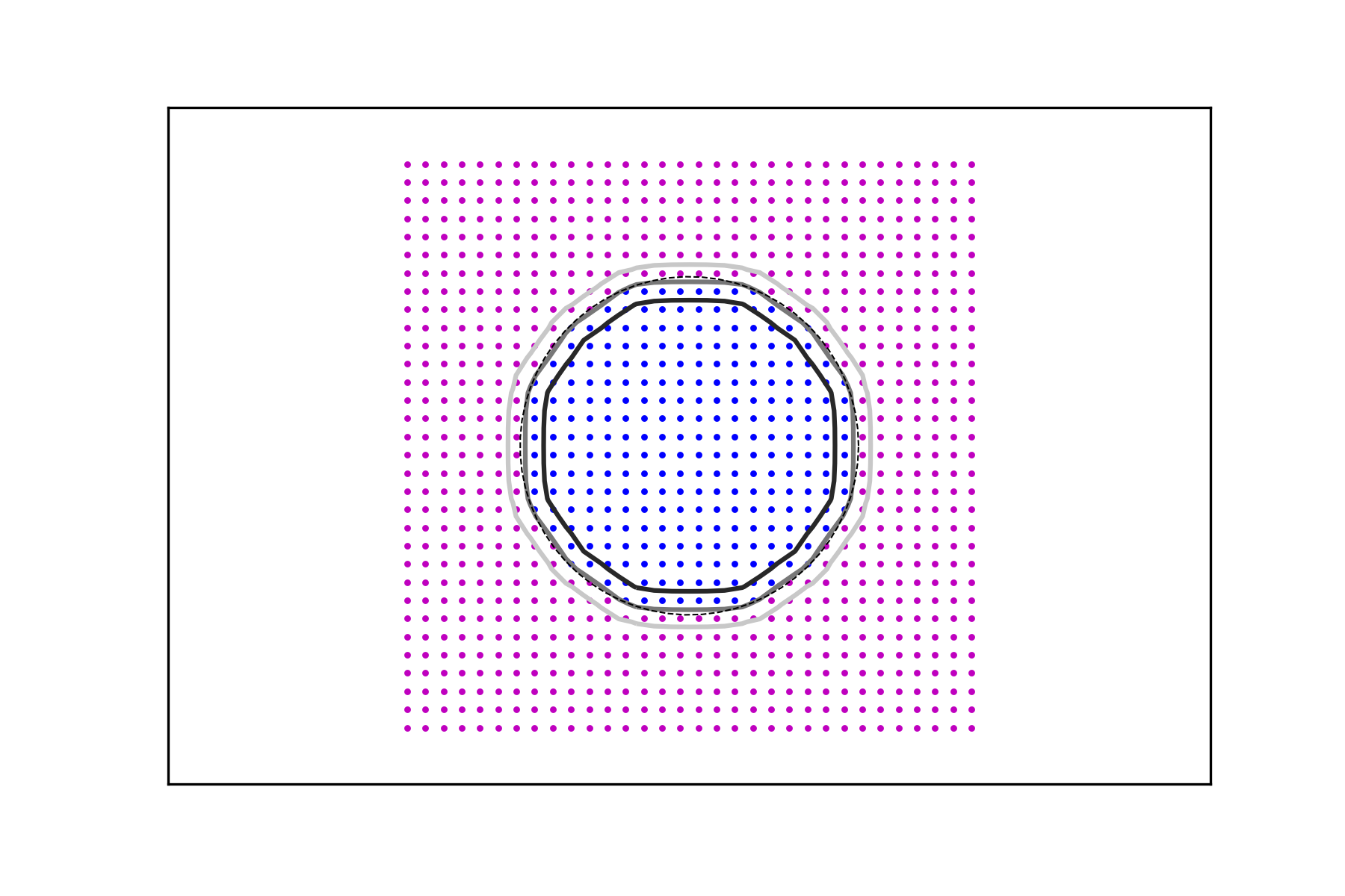
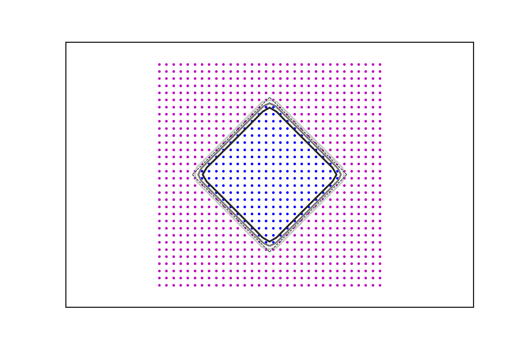
3.2. Characteristic Functions of Sets of Positive Measure

Take the three subsets of $\mathbb{R}^{2}$

$$S_{1} =\big{\{}x\in\mathbb{R}^{2}\,\big{|}\,|x|\leq.6\big{\}},$$ (3.1)

$$S_{2} =\big{\{}x\in\mathbb{R}^{2}\,\big{|}\,|x_{1}|+|x_{2}|\leq.7\big{\}},$$ (3.2)

$$S_{3} =\big{\{}r(\theta)\bigl{(}\cos(\theta),\sin(\theta)\bigr{)}\in\mathbb{R}^{2}\,\big{|}\,.4\leq r(\theta)\leq.6+.1\cos(4\theta),\>\theta\in[0,2\pi)\big{\}},$$ (3.3)

and consider the associated characteristic function $\chi_{S_{j}}$ for $j=1,2,3$. The first data set consists of the values of these functions on a regular grid, that is,

$$\mathbb{D}_{m,j}=\big{\{}\bigl{(}x^{i},\chi_{S_{j}}(x^{i})\bigr{)}\,\big{|}\,i=1,\dots,m^{2}\big{\}},\>j=1,2,3,$$

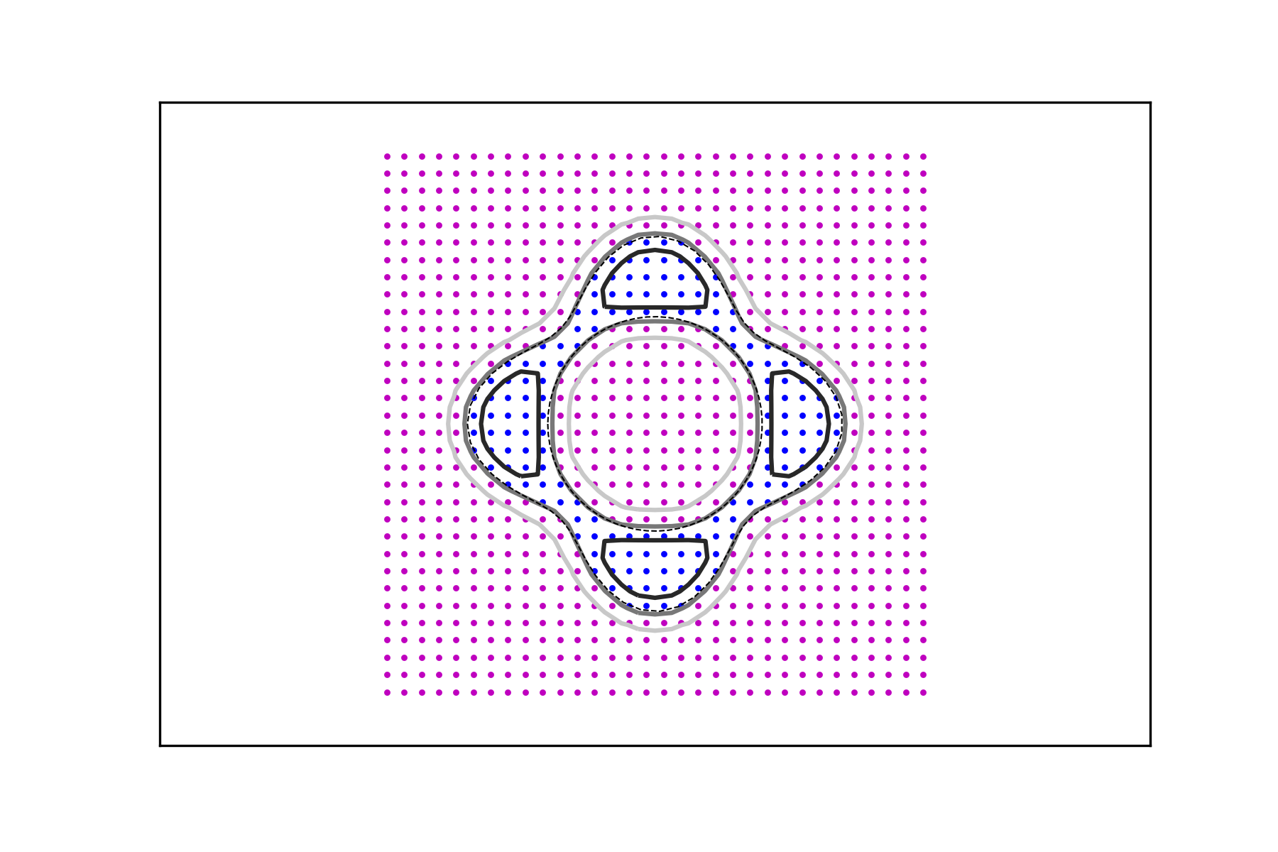
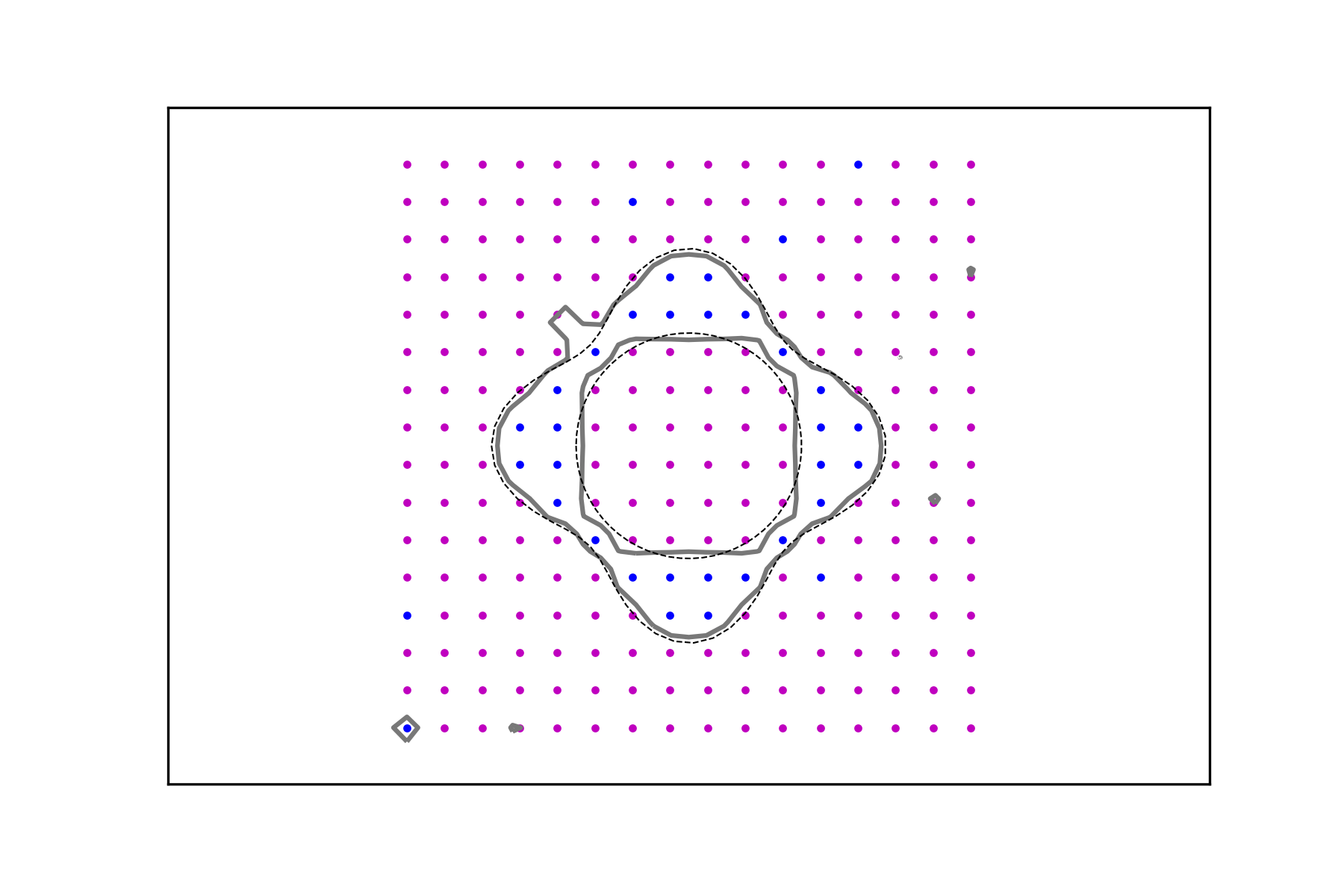
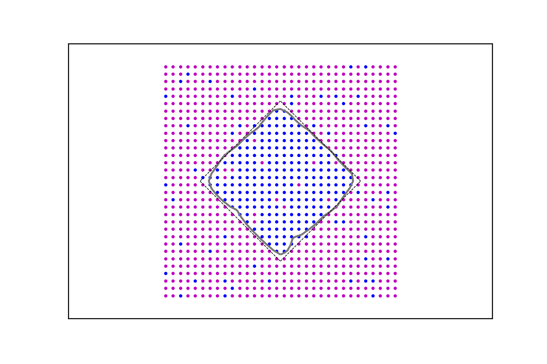
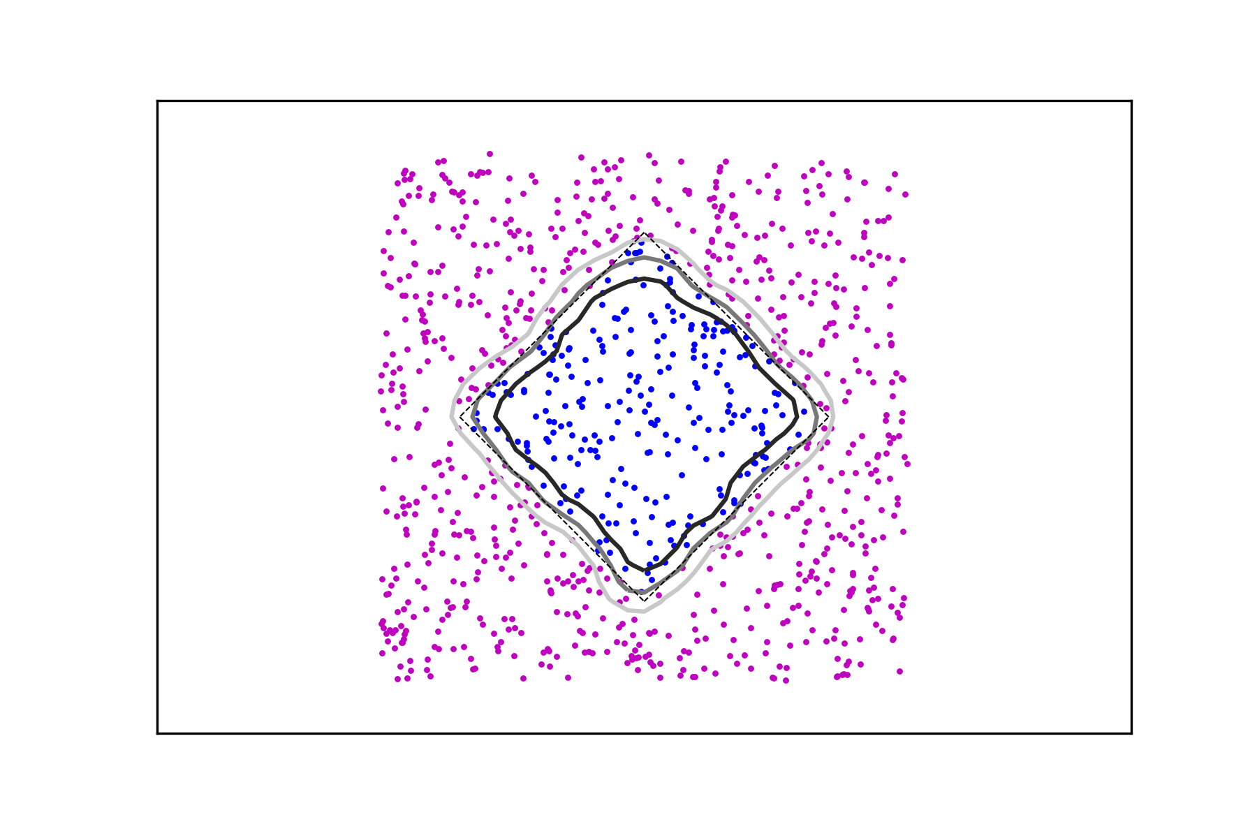
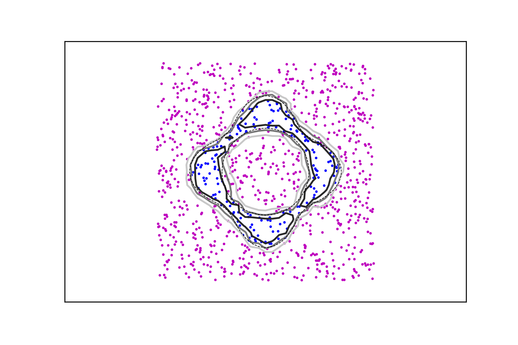
for $\mathbb{X}_{m}=\big{\{}(kh-1,lh-1)\,\big{|}\,0\leq k,l\leq m-1\big{\}}$ and $h=2/(m-1)$, which amounts to a uniform discretization of the box $B=[-1,1]\times[-1,1]$. In Figure 1 some level lines of the interpolant $u_{\mathbb{D}_{m,j}}$ are shown for the three functions $\chi_{S_{j}}$, $j=1,2,3$, and for different values of the regularizing parameter $\alpha>0$ and $m=16$. While the size of the data set clearly correlates with the “accuracy” of the interpolation, the approximating function does an excellent job at generating meaningful and smooth level sets. Their smoothness is affected mainly by the parameter $\alpha$ and the their proximity to the level sets corresponding to the highest values.

Figure 1. Level lines of the signal $u_{\mathbb{D}_{m,j}}$ for $m=16$, $j=1,2,3$, and $\alpha=0,1,1,2$. Depicted are the data set (blue dots correspond to the value 1 while magenta dots to the value 0) and three level lines corresponding to levels at 20%, 50%, and 80% of the signal’s maximal value, respectively. Darker lines correspond to higher levels. The parameter $\alpha$ grows from left to right. The boundary of the set $S_{j}$ appears as a dashed black line.

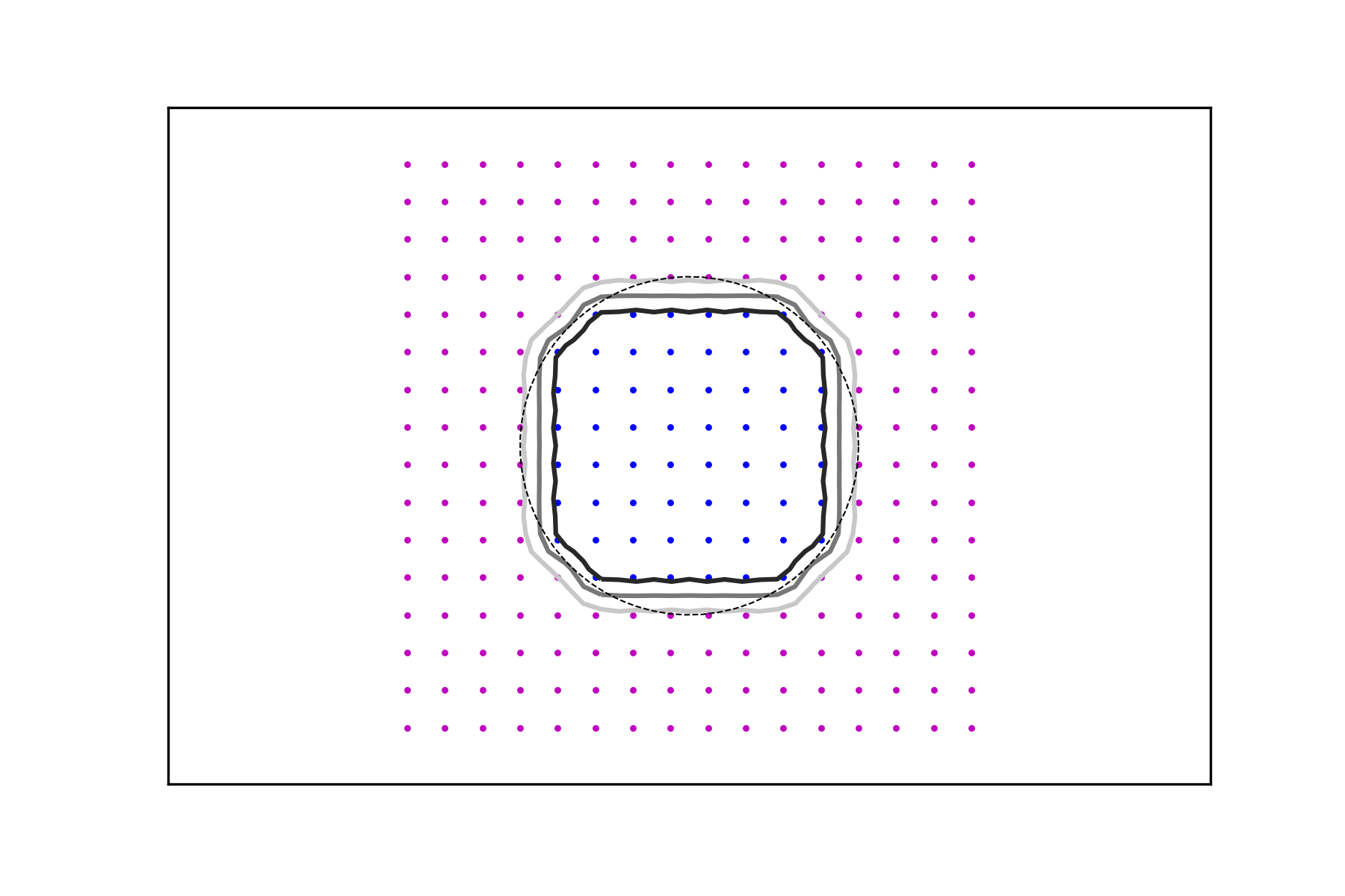
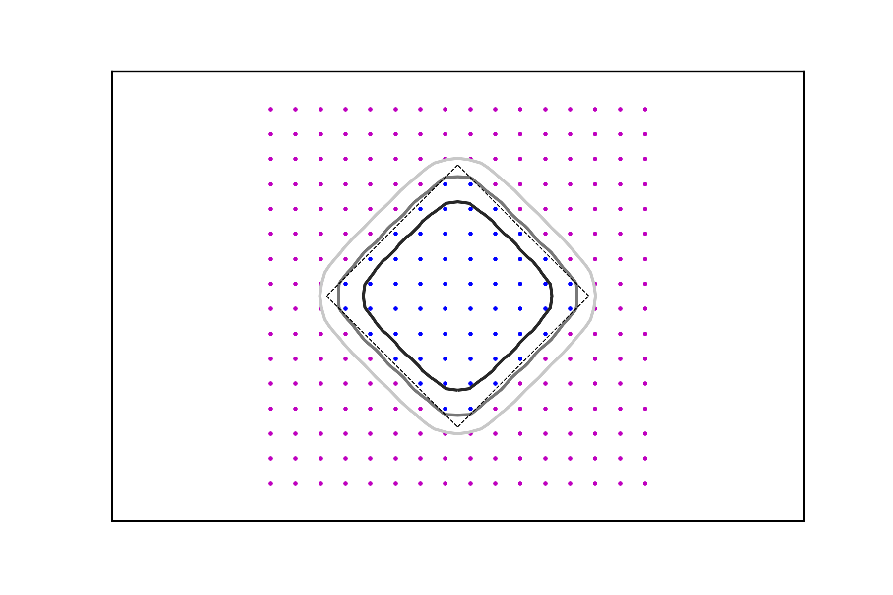
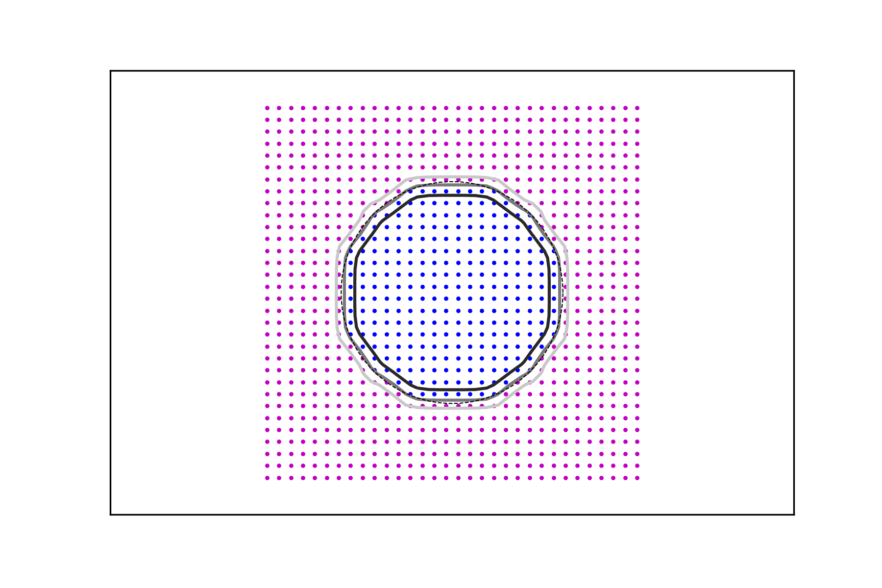
It follows that if a characteristic function has to be recovered or inferred from a data set, thresholding based on the interpolant $u_{\mathbb{D}_{m,j}}$ is an effective strategy and the decision boundary $\bigl{[}u_{\mathbb{D}_{m,j}}=.5\max(u_{\mathbb{D}_{m,j}})\bigr{]}$ is a solid choice across a range of values of the regularization parameter. Figure 2 depicts the same experiments using the denser data sets $\mathbb{D}_{32,j}$ for $j=1,2,3$.

Figure 2. Level lines of the signal $u_{\mathbb{D}_{m,j}}$ for $m=32$, $j=1,2,3$, and $\alpha=0,1,1,2$. Depicted are the data set (blue dots correspond to the value 1 while magenta dots to the value 0) and three level lines corresponding to levels at 20%, 50%, and 80% of the signal’s maximal value, respectively. Darker lines correspond to higher levels. The parameter $\alpha$ grows from left to right. The boundary of the set $S_{j}$ appears as a dashed black line.

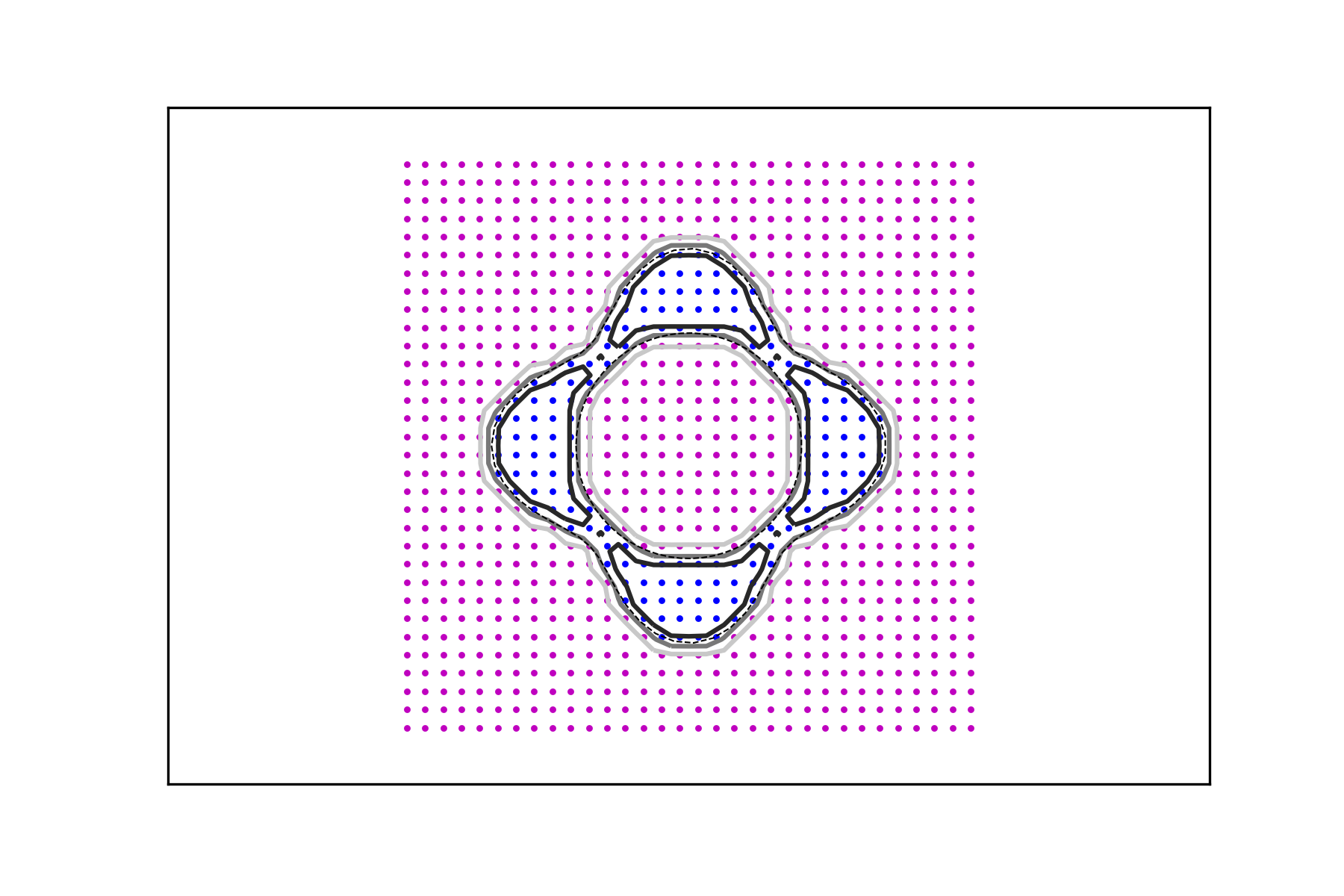
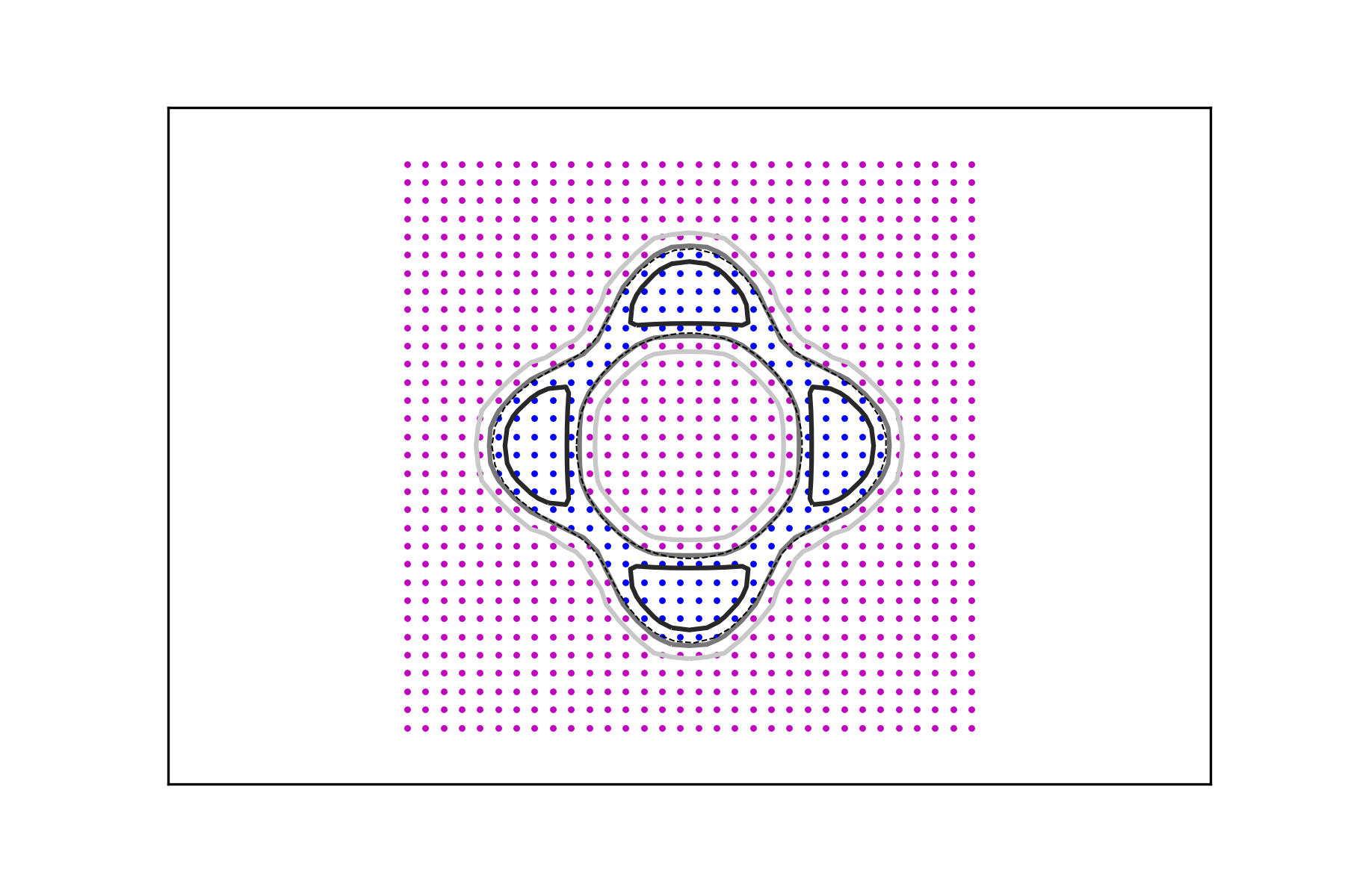
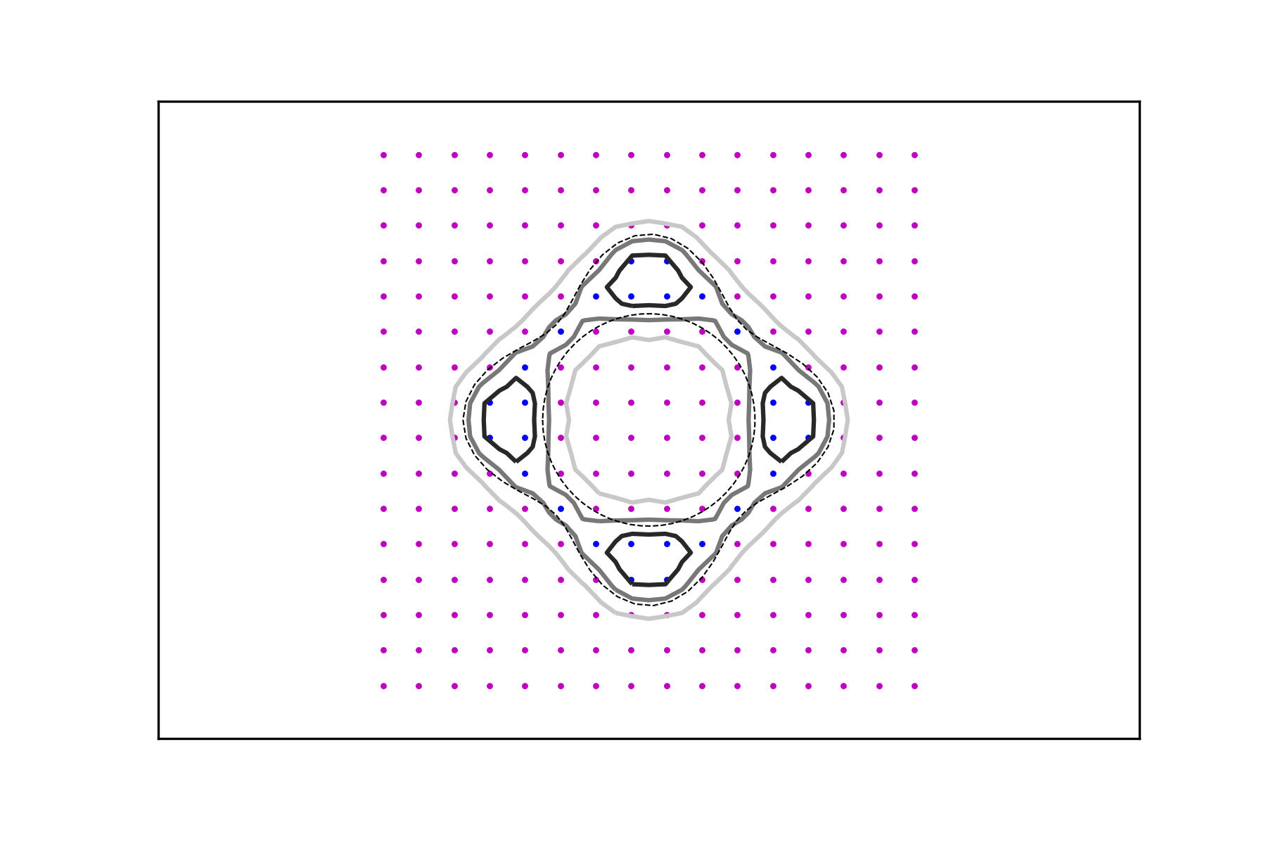
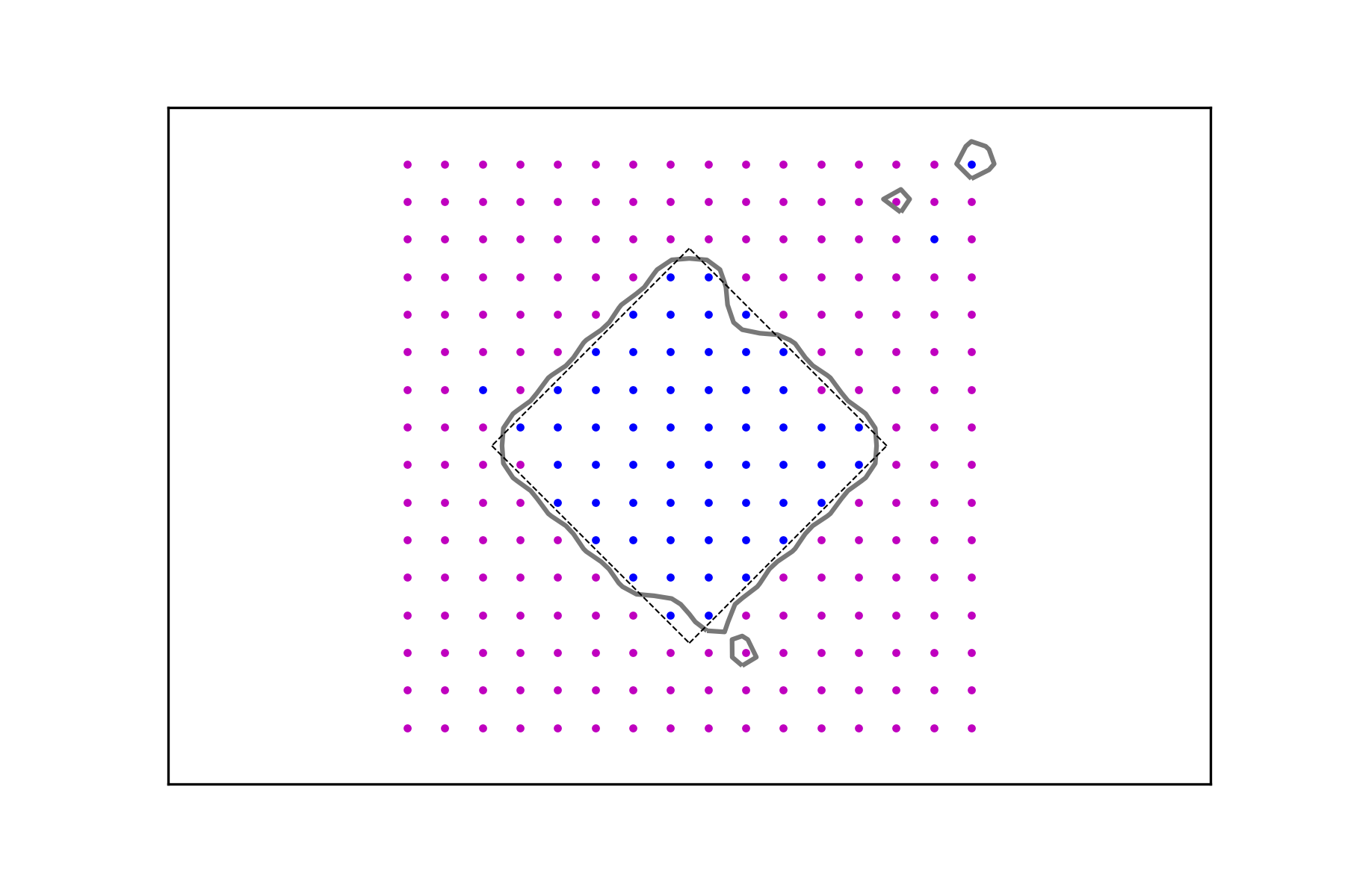
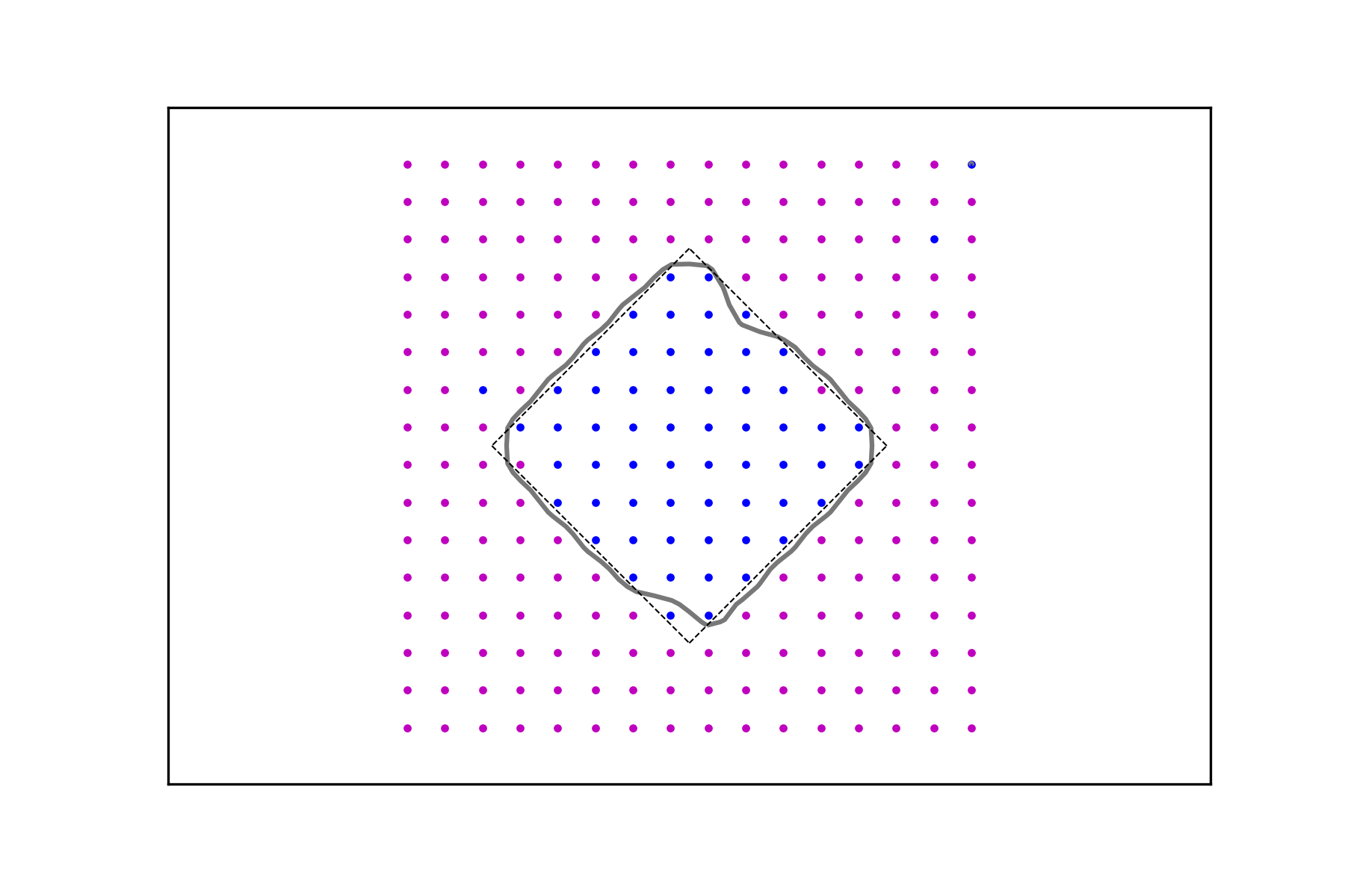
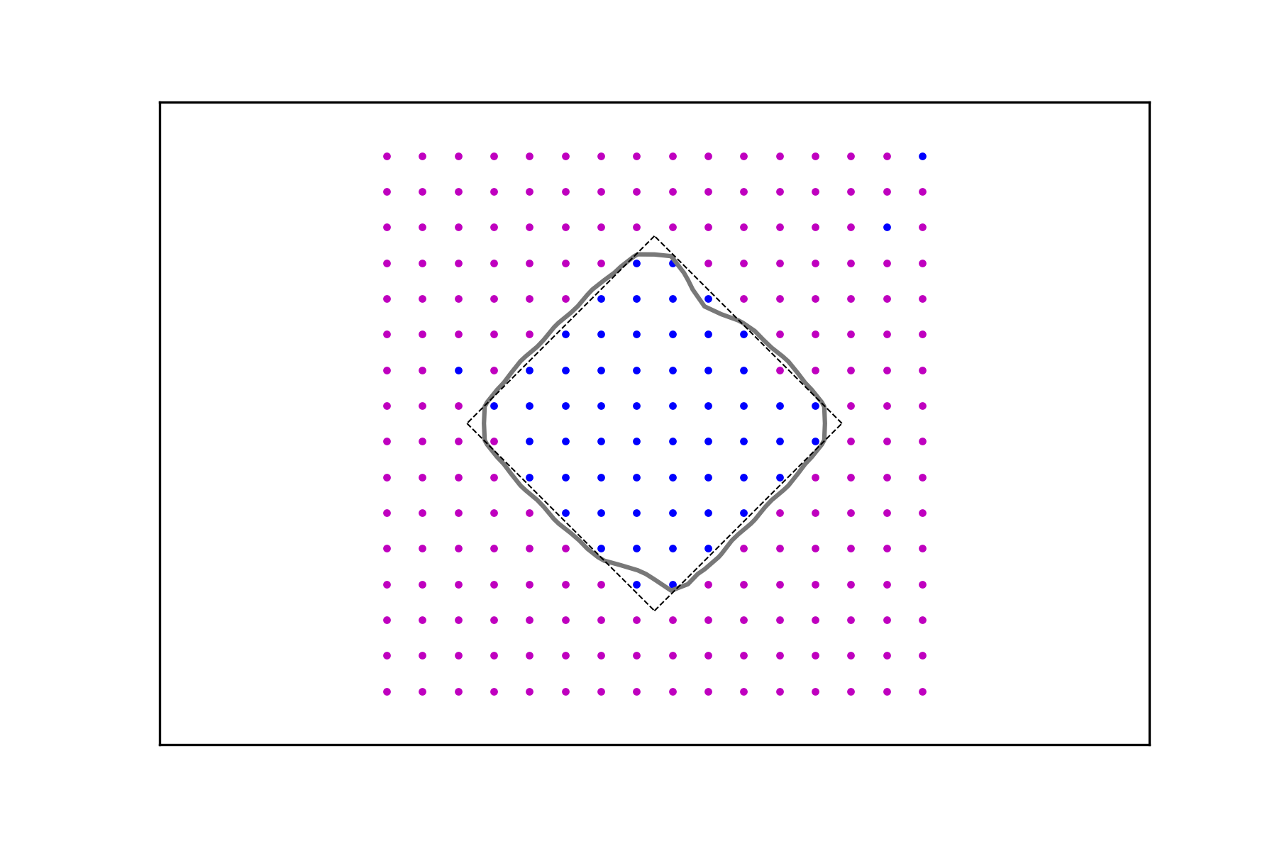
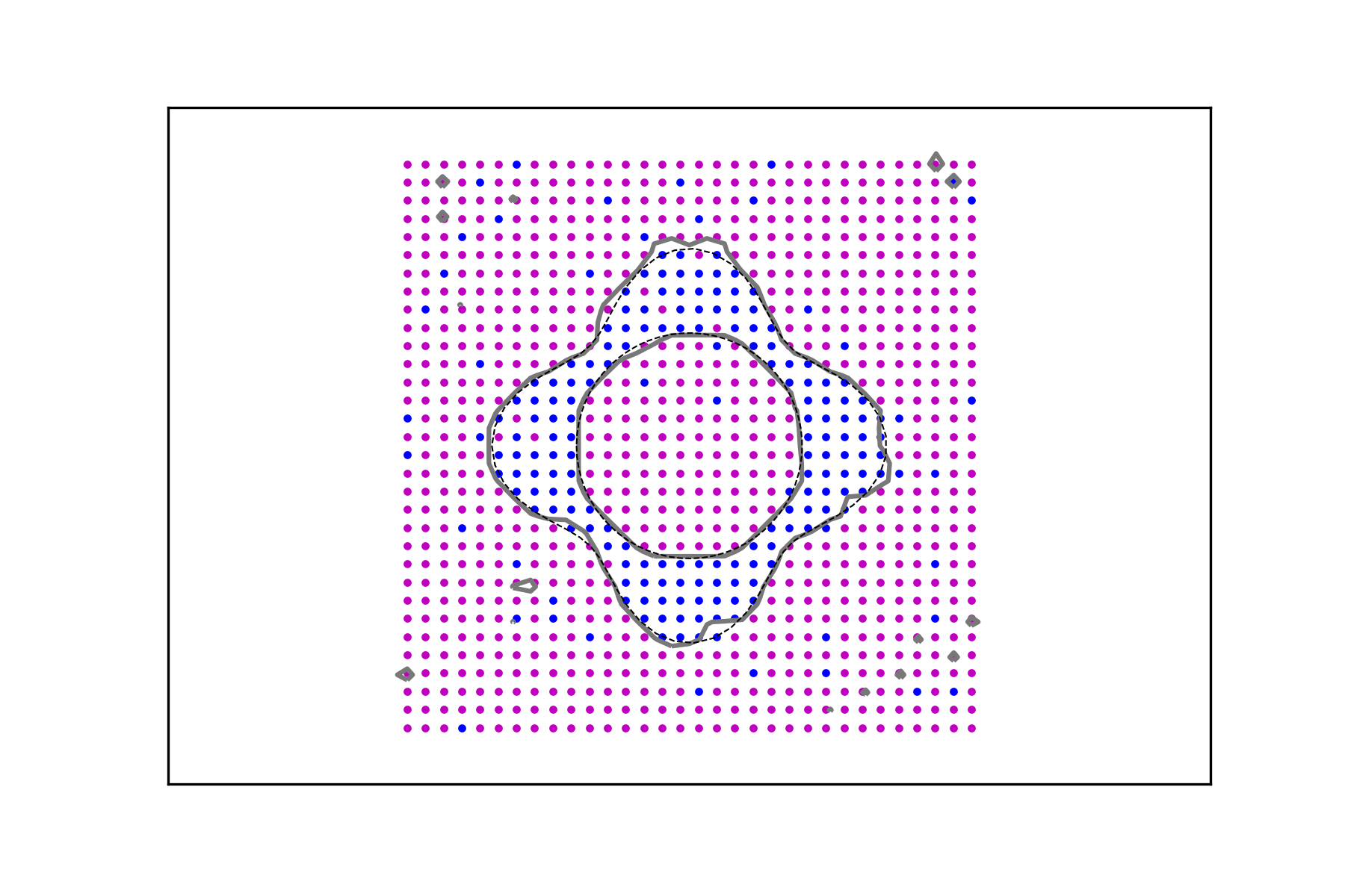
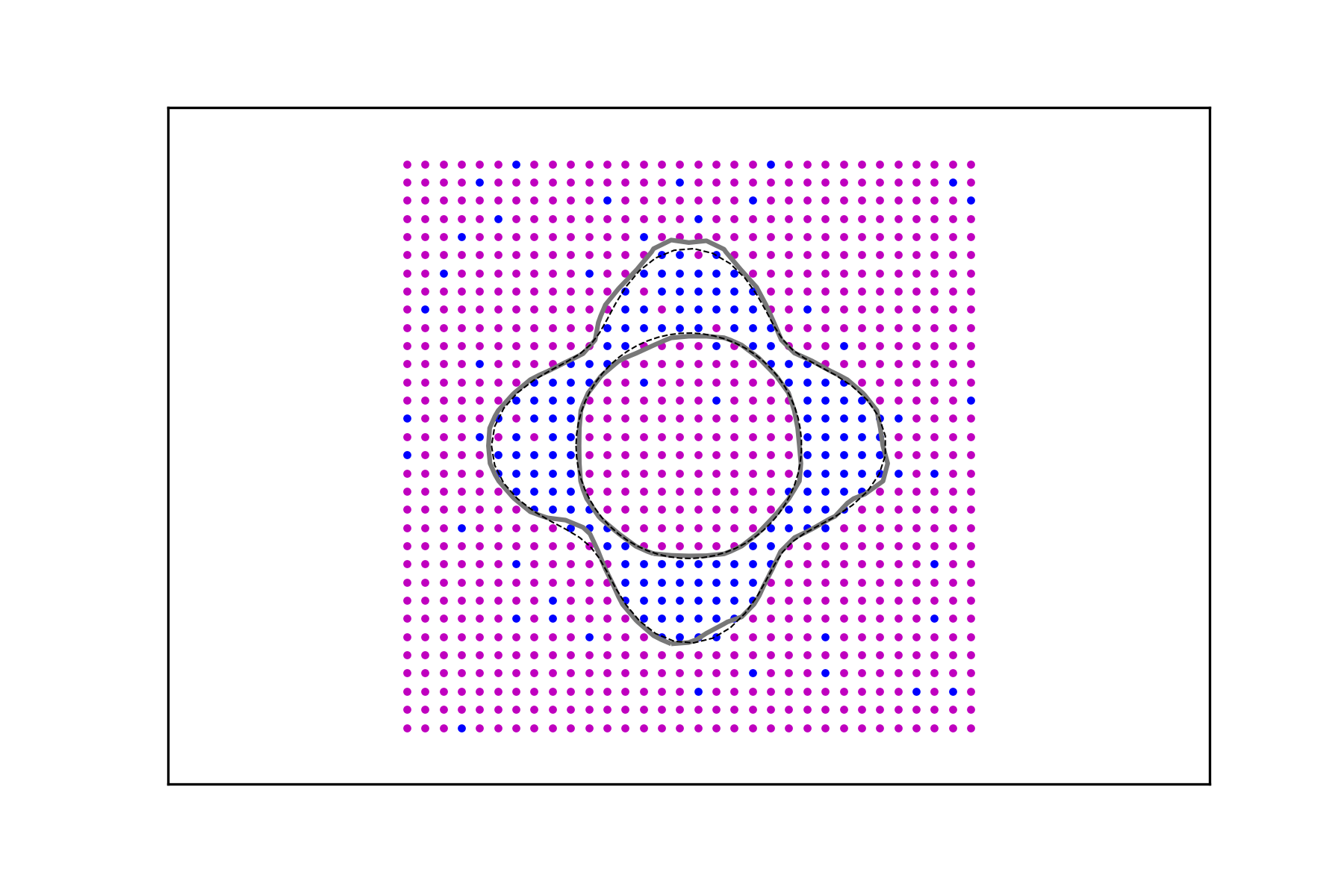
In Figures 3 and 4, it is shown how the method performs in the presence of data corruption. In Figure 3 2% of the data is misclassified, whereas the misclassification rate in Figure 4 is 5%. By this we mean that a mistake is made, with the given probability, when a value is assigned to an argument by evaluating the corresponding characteristic function. These examples clearly demonstrate the usefulness of the regularizing parameter which leads to data signals whose decision level sets are more stable in the presence of classification errors.

Figure 3. Decision boundary of the signal $u_{\mathbb{D}_{m,j}}$ for $m=16$, $j=2,3$, and $a=0,1,1,2$ with 2% data corruption rate. Depicted are the data set (blue dots correspond to the value 1 while magenta dots to the value 0) and the level line corresponding to 50% of the signal’s maximal value. The parameter $\alpha$ grows from left to right. The boundary of the set $S_{j}$ appears as a dashed black line.

Figure 4. Decision boundary of the signal $u_{\mathbb{D}_{m,j}}$ for $m=32$, $j=2,3$, and $a=0,1,1,2$ with 5% data corruption rate. Depicted are the data set (blue dots correspond to the value 1 while magenta dots to the value 0) and the level line corresponding to 50% of the signal’s maximal value. The parameter $\alpha$ grows from left to right. The boundary of the set $S_{j}$ appears as a dashed black line.

3.3. Sample Data

Finally we demonstrate that the method offers a degree robustness when the data arguments are randomly sampled from a uniform distribution supported on the box $B$. The resulting decision boundaries of half maximal value are depicted in Figure 5 along with the sampled argument data sets $\mathbb{X}_{m}$. The sampling rate clearly affects the smoothness of the level sets, a deterioration that is to some extent counteracted by the regularization.

Figure 5. Level lines of 20%, 50%, and 80%, increasingly dark, of the signal’s maximal value for regularizations parameter $\alpha=.1,1,2.$, from left to right. The number of randomly sampled points, also depicted with the associated value color-coded (with blue representing the value 1, while magenta the value 0), is $1024$ as in the denser regular grids of previous examples.

3.4. Classification

Continuity of the interpolant and its level sets (almost all of them actually smooth) are obtained at the cost of approximate interpolation. Such an approximation can still be accurate when the argument data set covers the function’s domain of definition uniformly and the value set is accurate, but the real advantage of this method is its applicability to incomplete data and/or noisy data sets. This point is further reinforced with the next series of experiments, where the data build a lower dimensional manifold of the ambient space and its signal is weak, that is, information about the underlying function is limited to sets of zero measure, or the data is not deterministic (in its argument set) but only has a probability distribution for its location.

Consider the data sets $\mathbb{D}_{k}$, $k=1,2$, consisting of points belonging to two distinct classes: points along a circle and points on the union of two segments with two different densities as depicted in Figure 6. For $k=1,2$, denote the circular data sets by

$$C_{k}=\big{\{}c^{i}_{k}\,\big{|}\,i=1,\dots m_{C_{k}}\big{\}}$$

and the union of segments data sets by

$$S_{k}=\big{\{}s^{i}_{k}\,\big{|}\,i=1,\dots m_{S_{k}}\big{\}}$$

Figure 6. From left to right, the data set pairs $(C_{k},S_{k})$, $k=1,2$. They can be thought as different samplings of the same pair of “continuous” sets.

In the spirit of the previous examples, we create two pairs of data sets

$$\mathbb{D}_{C_{k}}=\big{\{}(c^{i}_{k},1)\,\big{|}\,i=1,\dots m_{C_{k}}\big{\}}\cup\big{\{}(s^{i}_{k},0)\,\big{|}\,i=1,\dots m_{S_{k}}\big{\}}\text{ and }$$

$$\mathbb{D}_{S_{k}}=\big{\{}(s^{i}_{k},1)\,\big{|}\,i=1,\dots m_{S_{k}}\big{\}}\cup\big{\{}(c^{i}_{k},0)\,\big{|}\,i=1,\dots m_{C_{k}}\big{\}},\>k=1,2$$

and compute the associated signals $u_{\mathbb{D}_{C_{k}}}$ and $u_{\mathbb{D}_{S_{k}}}$, $k=1,2$. Figure 7 shows the level sets

$$[u_{\mathbb{D}_{C_{k}}}=.5\max(u_{\mathbb{D}_{C_{k}}})\bigr{]}\text{ and }[u_{\mathbb{D}_{S_{k}}}=.5\max(u_{\mathbb{D}_{S_{k}}})\bigr{]},\>k=1,2.$$

for different values of the regularization parameter.

Figure 7. The 50% of maximum level lines for the signals $u_{\mathbb{D}_{C}}$ and $u_{\mathbb{D}_{S}}$ of the data sets based on the two data classes $C_{k}$ and $S_{k}$ for $k=1,2$. The first two rows correspond to $k=1$ and the second two to $k=2$. Withing each row, from left to right, the regularization parameter is $\alpha=.1,1,2$.

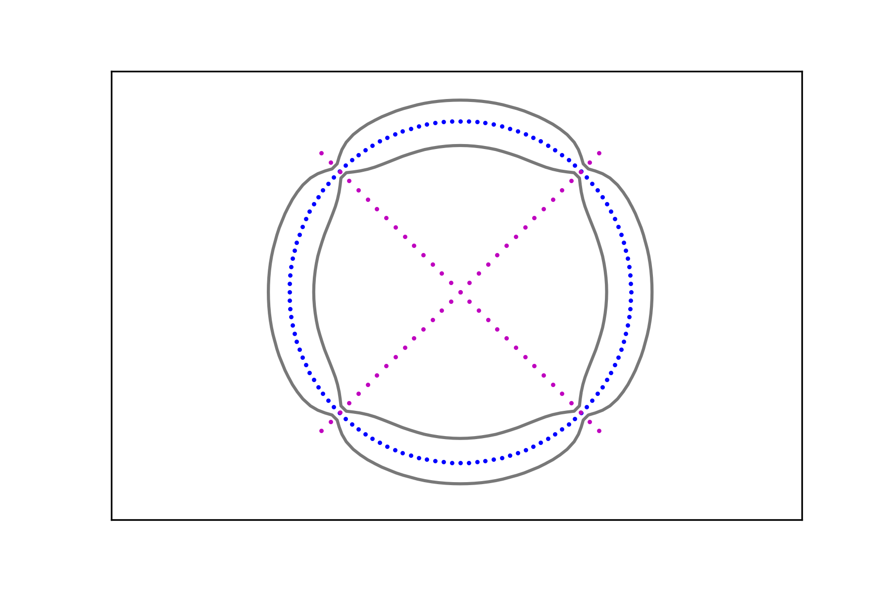
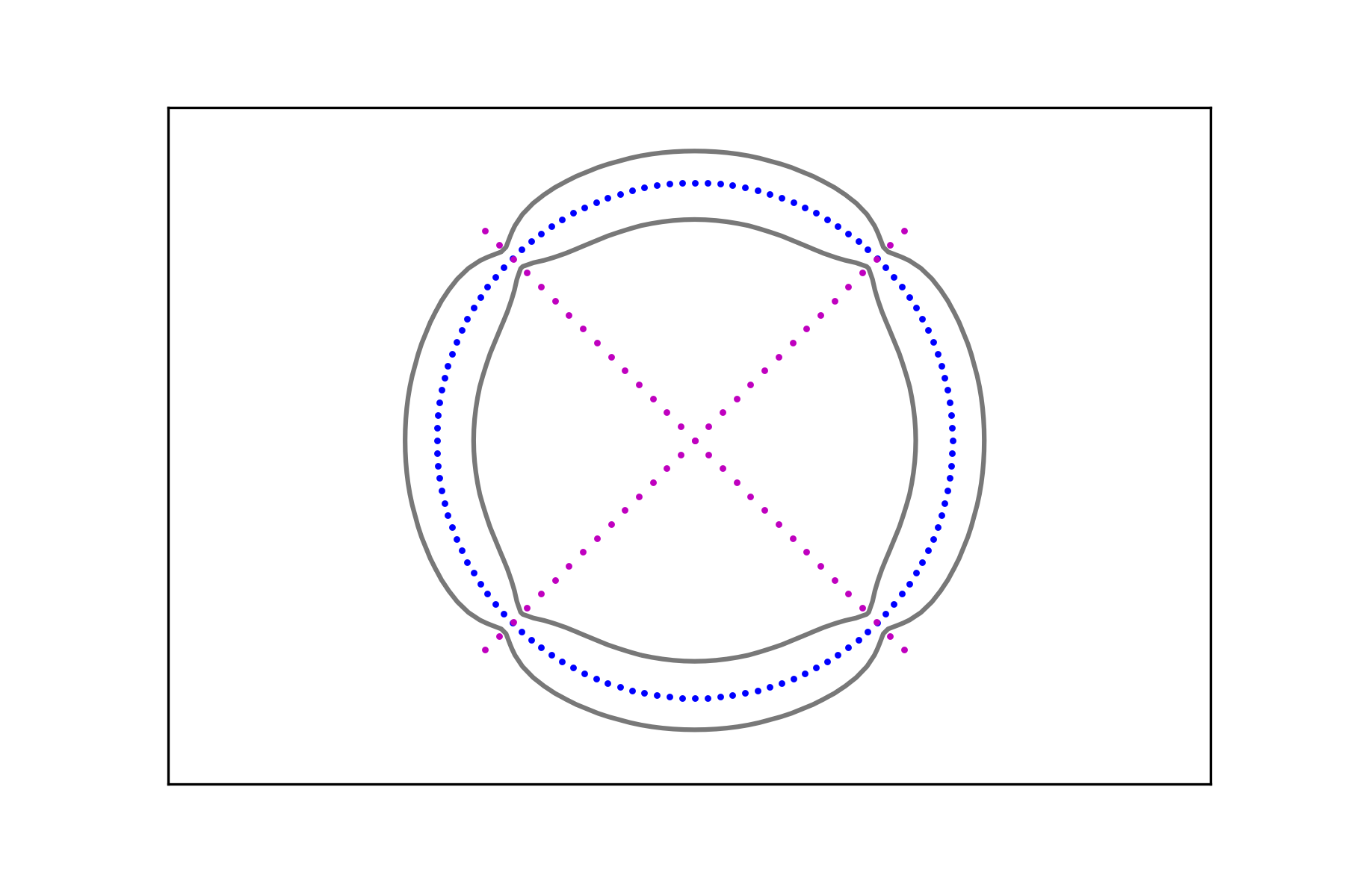
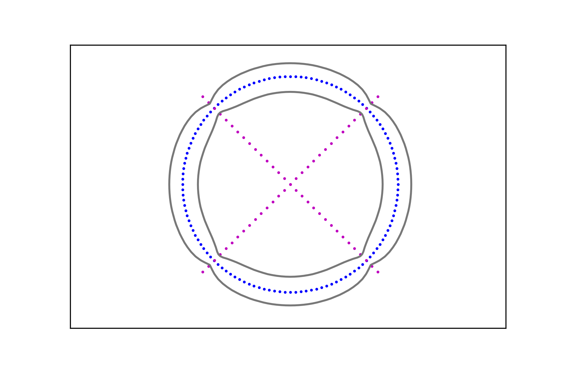
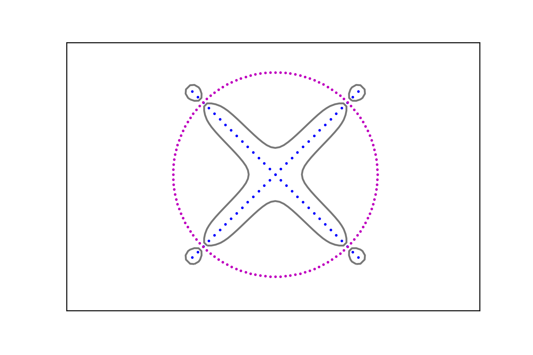
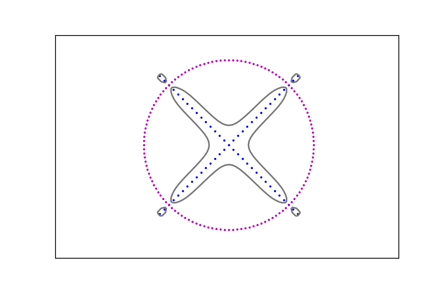
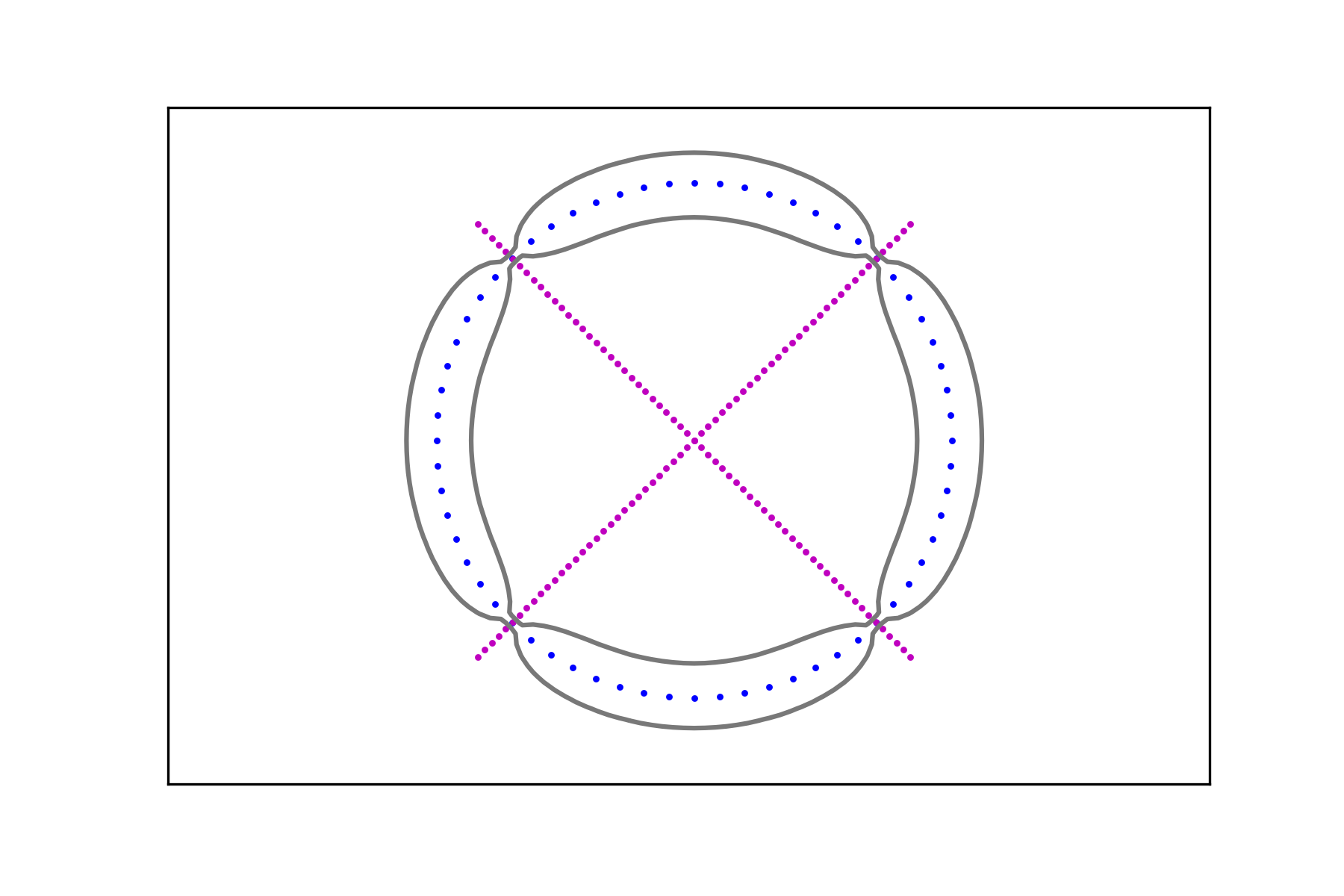
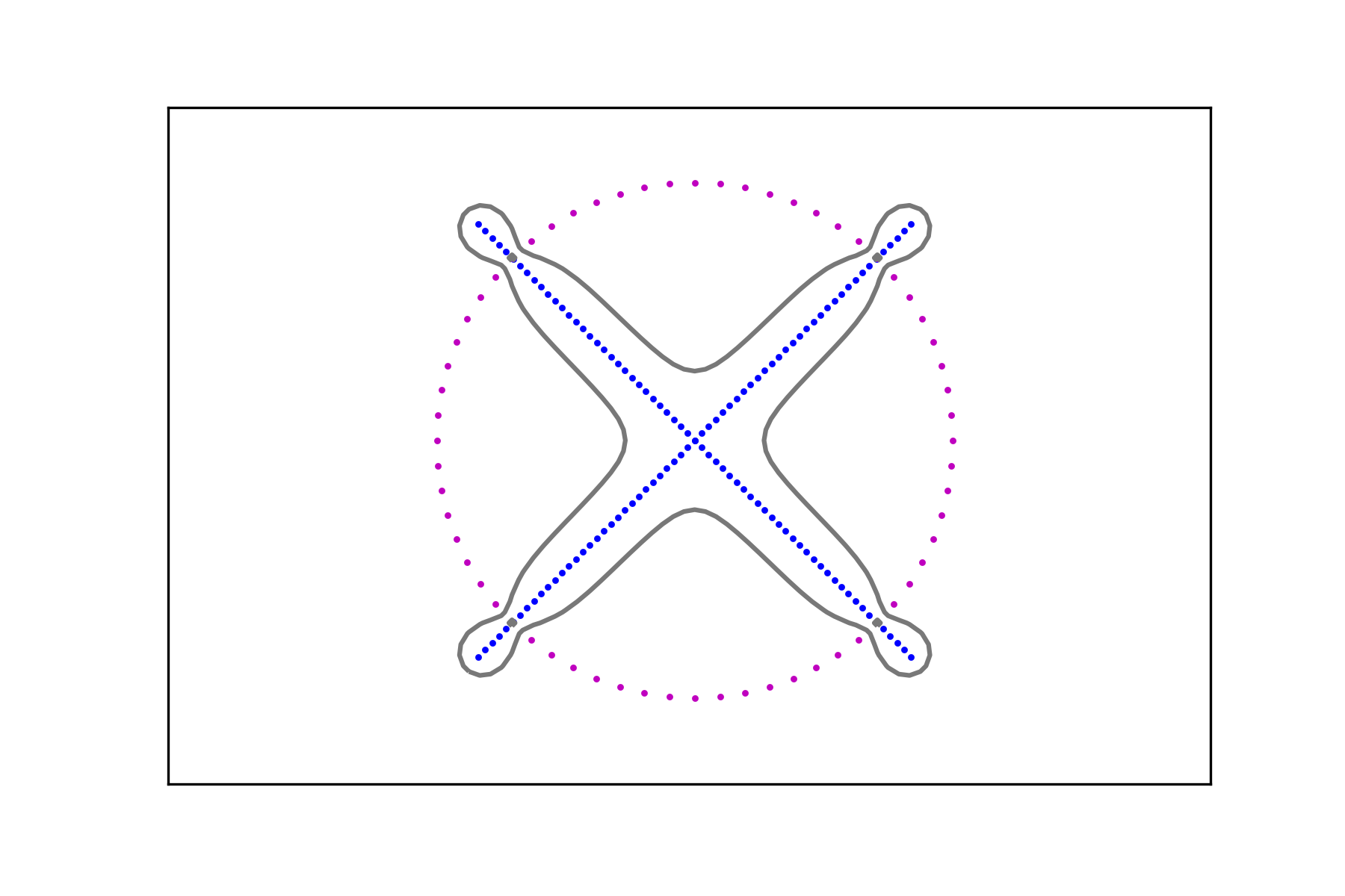
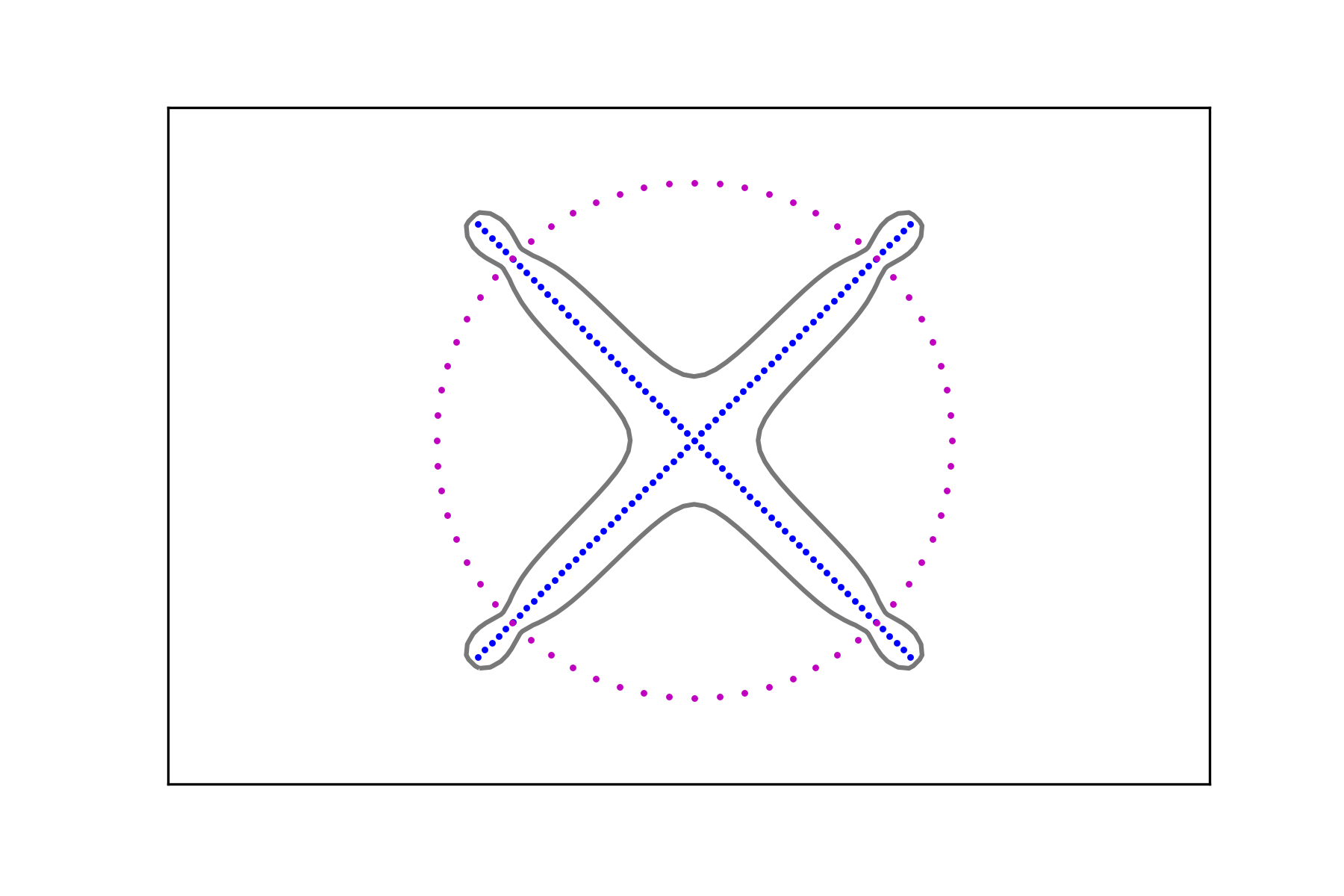
The region in their interior (i.e. the one containing the corresponding data set) can be considered as a smooth fattening of the data set to a set of positive measure. It can be obtained for any data set regardless of the intensity of its signal.

Next we turn our interest to the question of classification: given a point $z\in\mathbb{R}^{2}$ that needs to be classified, we use the decision algorithm defined by (2.7). This gives

$$L(z)=\operatorname{argmax}_{l=1,2}u_{\mathbb{D}_{l}}(z),$$

which, in this case, yields the level lines (hypersurfaces in higher dimension)

$$\bigl{[}u_{\mathbb{D}_{1}}=u_{\mathbb{D}_{2}}\bigr{]}$$ (3.4)

as the decision boundary. This is illustrated in Figure 8 for the classification problem of the two class pairs $(C_{k},S_{k})$ for $k=1,2$ introduced above.

Figure 8. The decision boundary computed according to (3.4) for two classes depicted in the same image. The $k$th row corresponds to the class pair $(C_{k},S_{k})$, $k=1,2$. Notice how the decision boundary is affected by the “density” of the data sets and not very strongly affected by the regularization parameter. The latter is, from left to right, $\alpha=.1,1,2$.

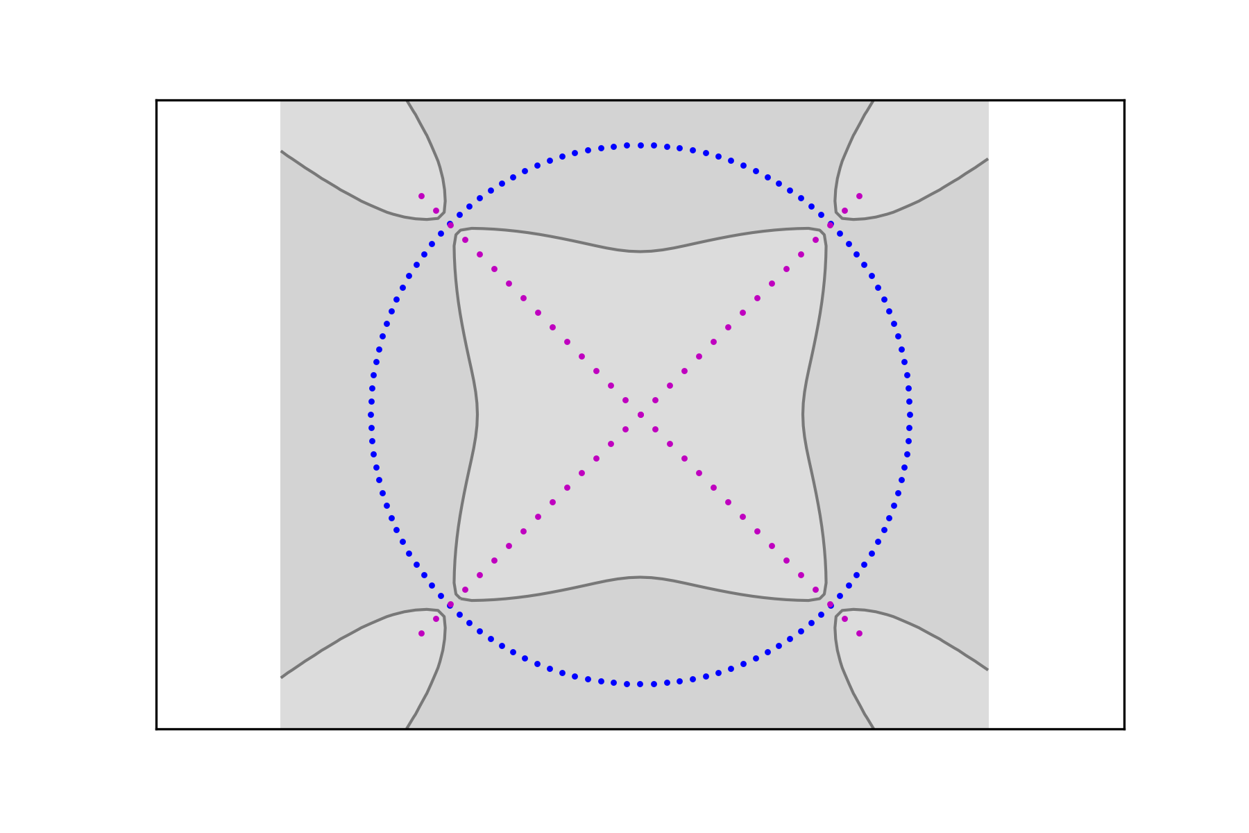
If the data pairs $(C_{k},S_{k})$, $k=1,2$, are considered the ground truth, then the above decision boundary is arguably optimal. If, on the other hand, it is known that the actual sets are the continuous circle and the union of two segments, then the data are only a sampling of these sets. In this case, the decision boundary may be biased by the relative oversampling of the one set compared to the other. This is evident when one compares the decision boundaries of Figure 8. In concrete situations, if information about the dimensionality of the ground truth is known, this effect can be mitigated by using comparable sampling rates for the different classes (see next section for an example of this procedure).

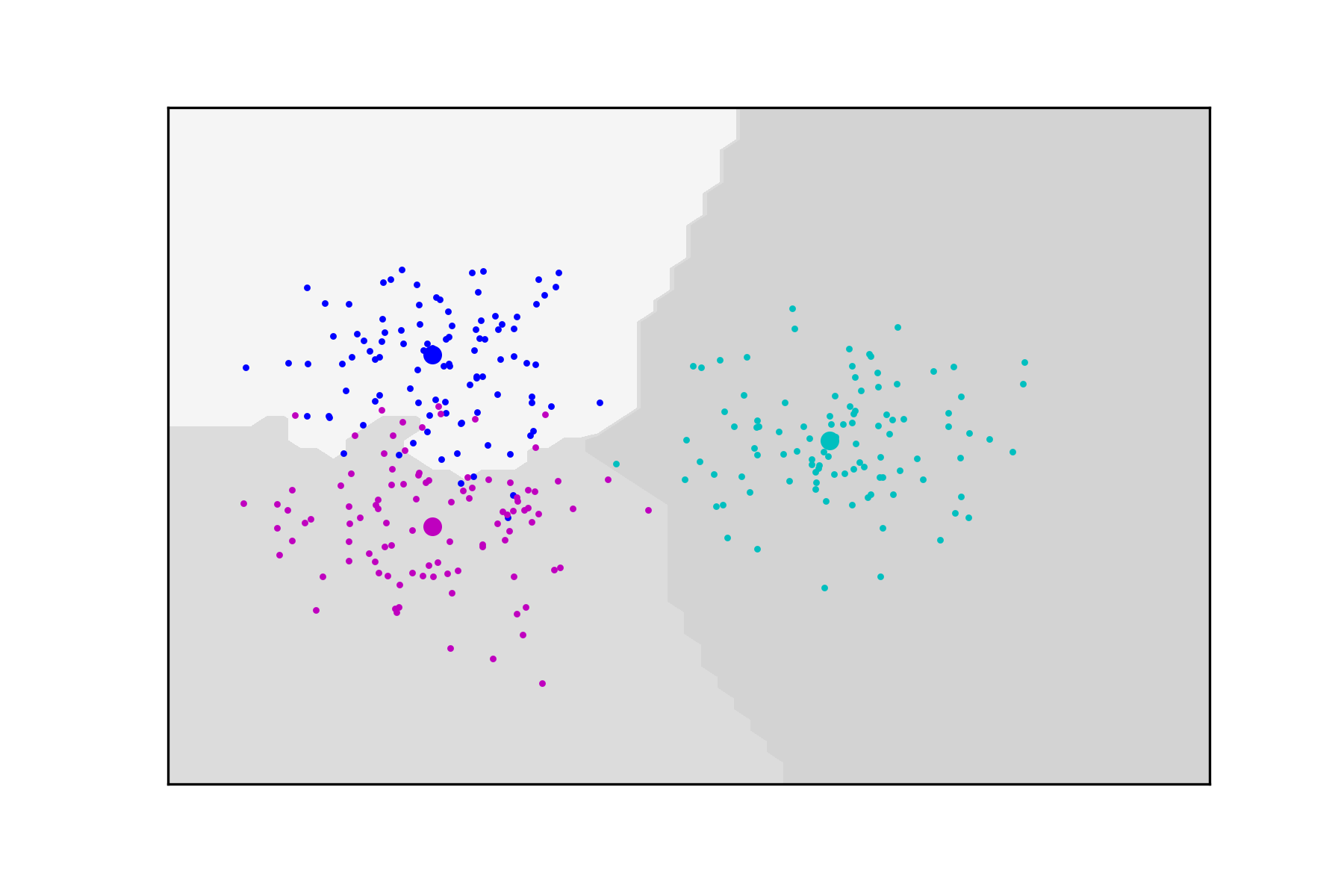
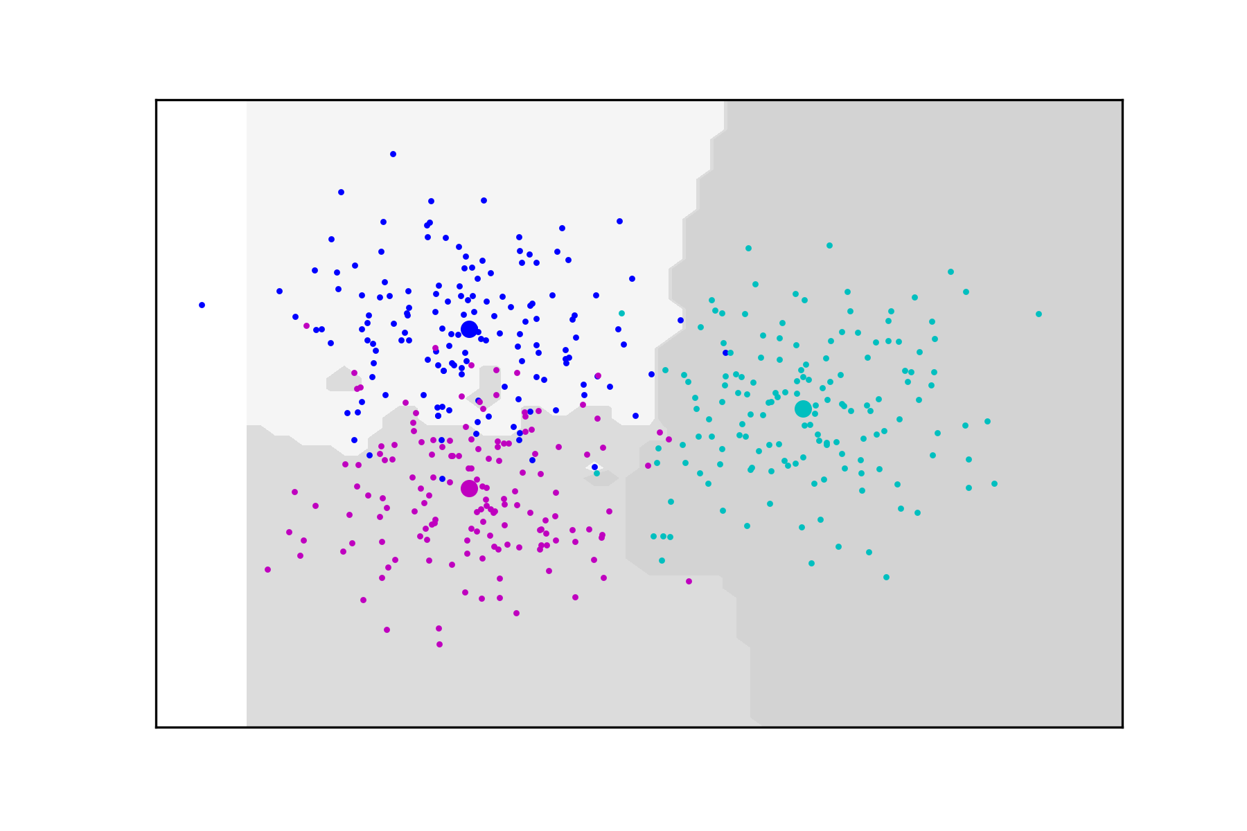
We conclude this section with a classification problem for data $\mathbb{X}_{0}$ split into three classes $\mathbb{X}_{l}$, $l=1,2,3$, each consisting of a set of points which are normally distributed with mean $p_{l}\in\mathbb{R}^{2}$ and different covariance matrices. The data set and the corresponding decision regions computed based on (2.7) are depicted in Figure 9. In these experiments $\alpha=1$.

Figure 9. The decision regions computed according to (2.7) for three classes of normally distributed points depicted using different colors in the same image. The average of each class is plotted as a large disk. The first row shows three different realization of the same three normal distributions and the computed decision regions. The first image in the second row is based on the same distributions as the first row but the sample size is increased, the second and third show the decision regions for different choices of means and covariance matrices. In all but the last example the covariance is taken to be diagonal. In the third and the last image, one of the sample points is outside the computational box where the data signals are generated and hence generated an unshaded region.

3.5. The MNIST data set

The final application is to the standard machine learning example and toy problem of digit classification for the MNIST data set. The data set consists of $28\times 28$ grayscale images of hand-written digits stored as vectors in $[0,255]^{784}$. Here it is considered that the ambient space is simply $\mathbb{R}^{784}$. The argument data is normalized to have unit Euclidean norm, that is, each original vector $x$ is replaced by $x/|x|$. In this way the maximal Euclidean distance between any two data points is $2\sqrt{2}$. The data set is split into a training set containing 60,000 data points $x$ and their corresponding label $d(x)$ indicating which digit is represented, and a testing data set of size 10,000. The labels of the testing data are known but need to be inferred from any knowledge that can be gleaned from the training set. This an example of when, due to the so-called curse of dimensionality, the data does not have any hope to fill the ambient space uniformly and thus, even if one assumed the existence of an underlying function $d:\mathbb{R}^{784}\to\{0,1,\dots,9\}$, the data would never be sufficient to accurately approximate it. It has to be said of course, that the testing data mostly does not stray away significantly from the training data and the different digits in the latter build thin subsets of the ambient space. This fact is typically captured by saying that the data lives in some lower dimensional manifold(s). We know from the previous section and from the two dimensional experiments, however, that the (training) data still generates a significant, if not strong, signal. The classification method described in the sequel exploits this signal and does not require any kind of training based on the minimization of non-convex functionals, as is often the case for machine learning algorithms based on neural nets. It is, in fact, based on the solution of low dimensional, well-posed linear systems as is about to be explained. First, in order to strengthen the signal somewhat, the training set is expanded to include rotations by $\pm 10^{\circ}$ and horizontal/vertical translations by $\pm 2$ pixels of each image. Then, given a test image $z$, the closest $5$ training images of each digit class are determined

$$\mathbb{X}=\big{\{}x^{i_{j}}\,\big{|}\,j=1,\dots,50\big{\}},$$

where $d(x^{i_{j}})=\lfloor j/5\rfloor$. The idea is now to use system (2.4) in order to produce approximate interpolants $u_{d}:=u_{\mathbb{D}_{d}}$ of the characteristic functions of each digit class given by the data set

$$\mathbb{D}_{d}=\big{\{}\bigl{(}x^{i_{j}},\delta_{d,d(x^{i_{j}})}\bigr{)}\,\big{|}\,j=1,\dots,50\big{\}},$$

where $d=0,\dots,9$, and

$$\delta_{d,\bar{d}}=\begin{cases}1,&d=\bar{d},\\ 0,&d\neq\bar{d}.\end{cases}$$

Finally the approximative characteristic functions $u_{d}$ will compete to determine the digit $d(z)$ to be associated with the test image $z$ via (2.7), in this case

$$d(z)=\operatorname{argmax}_{d}u_{d}(z).$$

This approach yields an accuracy of $98.56\%$ on the test set. In Table 1 we record the detailed outcome of the classification, performed with $\alpha=1.5$.

Recall that this method is stable and depends continuously on the data set and hence delivers a robustness that methods with higher classification rates typically do not. Unlike neural networks it, moreover, does not require any training but uses the training set directly in a fully transparent way.

	0	1	2	3	4	5	6	7	8	9
0	973	0	1	0	0	2	3	1	0	0
1	0	1131	2	1	0	0	0	1	0	0
2	4	1	1015	0	1	0	0	10	0	1
3	0	0	1	995	0	8	0	3	3	0
4	0	0	0	0	971	0	4	1	0	6
5	1	0	0	8	0	877	4	1	0	1
6	0	2	0	0	0	1	955	0	0	0
7	0	4	4	0	0	0	0	1020	0	0
8	2	0	3	9	3	2	3	4	946	2
9	1	2	1	4	9	7	0	10	2	973

Table 1. MNIST classification results: the $k$th row of the table indicates in column $j$ how many times the digit $k$ is assigned the label $j$ by the algorithm.

Remark 3.1.

It should be pointed out that the proposed classification method performs well when the data classes effectively lie on submanifolds the shape of which their relative signals are able to capture. If the class similarity is not geometric in this sense, this method will likely not produce satisfactory results if applied to the original data. It is indeed possible for general data sets to exhbit classes that share some common feature but are far apart as points in space. In this case, the dots cannot be easily connected.

References

- [1] Mark A. Aizerman, Emmanuel M. Braverman, and Lev I. Rozonoer. Theoretical foundations of the potential function method in pattern recognition learning. Automation and Remote Control, 25:821–837, 1964.
- [2] Bernhard E. Boser, Isabelle M. Guyon, and Vladimir N. Vapnik. A training algorithm for optimal margin classifiers. In Proceedings of the fifth annual Acm workshop on Computational learning theory, pages 144–. Assn for Computing Machinery, 1992.
- [3] T. Poggio and F. Girosi. Regularization Algorithms for Learning that are Equivalent to Multilayer Networks. Science, 247(4945):978–982, 1990.
- [4] V.N. Vapnik and A.Y. Chervonenkis. On a class of algorithms of learning pattern recognition. Avtomatika i Telemekhanika, 25(6):In Russian, 1964.
- [5] H. Wendland. Scattered Data Approximations. Cambridge Monographs on Applied and Computational Mathematics. Cambridge University Press, Cambridge, 2004.