Contents
What is Contrastive Learning?
How does Contrastive Learning Work?
Loss Functions in Contrastive Learning
Contrastive Learning: Use Cases
Popular Contrastive Learning Frameworks
Contrastive Learning: Key Takeaways
Encord Blog
Full Guide to Contrastive Learning


Contrastive learning allows models to extract meaningful representations from unlabeled data.
By leveraging similarity and dissimilarity, contrastive learning enables models to map similar instances close together in a latent space while pushing apart those that are dissimilar.
This approach has proven to be effective across diverse domains, spanning computer vision, natural language processing (NLP), and reinforcement learning.
What is Contrastive Learning?
Contrastive learning is an approach that focuses on extracting meaningful representations by contrasting positive and negative pairs of instances. It leverages the assumption that similar instances should be closer in a learned embedding space while dissimilar instances should be farther apart. By framing learning as a discrimination task, contrastive learning allows models to capture relevant features and similarities in the data.
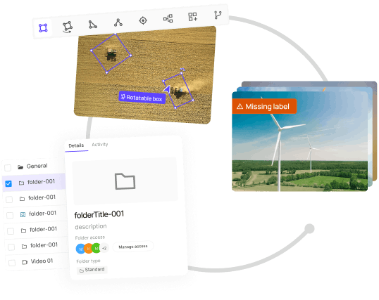
Supervised Contrastive Learning (SCL)
Supervised contrastive learning (SCL) is a branch that uses labeled data to train models explicitly to differentiate between similar and dissimilar instances. In SCL, the model is trained on pairs of data points and their labels, indicating whether the data points are similar or dissimilar. The objective is to learn a representation space where similar instances are clustered closer together, while dissimilar instances are pushed apart.
The Information Noise Contrastive Estimation (InfoNCE) loss function is a popular method. InfoNCE loss maximizes the agreement between positive samples and minimizes the agreement between negative samples in the learned representation space. By optimizing this objective, the model learns to discriminate between similar and dissimilar instances, leading to improved performance on downstream tasks.
We will discuss the InfoNCe loss and other losses later in the article.
Self-Supervised Contrastive Learning (SSCL)
Self-supervised contrastive learning (SSCL) takes a different approach by learning representations from unlabeled data without relying on explicit labels. SSCL leverages the design of pretext tasks, which create positive and negative pairs from the unlabeled data. These pretext tasks are carefully designed to encourage the model to capture meaningful features and similarities in the data.
One commonly used pretext task in SSCL is the generation of augmented views. This involves creating multiple augmented versions of the same instance and treating them as positive pairs, while instances from different samples are treated as negative pairs. Training the model to differentiate between these pairs, it learns to capture higher-level semantic information and generalize well to downstream tasks.
SSCL has shown impressive results in various domains, including computer vision and natural language processing. In computer vision, SSCL has been successful in tasks such as image classification, object detection, and image generation. SSCL has been applied to tasks like sentence representation learning, text classification, and machine translation in natural language processing.
Supervised Contrastive Learning
How does Contrastive Learning Work?
Contrastive learning has proven a powerful technique, allowing models to leverage large amounts of unlabeled data and improve performance even with limited labeled data. The fundamental idea behind contrastive learning is to encourage similar instances to be mapped closer together in a learned embedding space while pushing dissimilar instances farther apart. By framing learning as a discrimination task, contrastive learning allows models to capture relevant features and similarities in the data.
Now, let's dive into each step of the contrastive learning method to gain a deeper understanding of how it works.
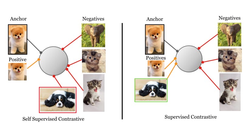
Data Augmentation
Contrastive learning often begins with data augmentation, which involves applying various transformations or perturbations to unlabeled data to create diverse instances or augmented views.
Data augmentation aims to increase the data's variability and expose the model to different perspectives of the same instance. Common data augmentation techniques include cropping, flipping, rotation, random crop, and color transformations. By generating diverse instances, contrastive learning ensures that the model learns to capture relevant information regardless of variations in the input data.
The Full Guide to Data Augmentation in Computer Vision
Encoder Network
The next step in contrastive learning is training an encoder network. The encoder network takes the augmented instances as input and maps them to a latent representation space, where meaningful features and similarities are captured.
The encoder network is typically a deep neural network architecture, such as a convolutional neural network (CNN) for image data or a recurrent neural network (RNN) for sequential data. The network learns to extract and encode high-level representations from the augmented instances, facilitating the discrimination between similar and dissimilar instances in the subsequent steps.
Projection Network
A projection network is employed to refine the learned representations further. The projection network takes the output of the encoder network and projects it onto a lower-dimensional space, often referred to as the projection or embedding space.
This additional projection step helps enhance the discriminative power of the learned representations. By mapping the representations to a lower-dimensional space, the projection network reduces the complexity and redundancy in the data, facilitating better separation between similar and dissimilar instances.
Contrastive Learning
Once the augmented instances are encoded and projected into the embedding space, the contrastive learning objective is applied. The objective is to maximize the agreement between positive pairs (instances from the same sample) and minimize the agreement between negative pairs (instances from different samples).
This encourages the model to pull similar instances closer together while pushing dissimilar instances apart. The similarity between instances is typically measured using a distance metric, such as Euclidean distance or cosine similarity. The model is trained to minimize the distance between positive pairs and maximize the distance between negative pairs in the embedding space.
Loss Function
Contrastive learning utilizes a variety of loss functions to establish the objectives of the learning process. These loss functions are crucial in guiding the model to capture significant representations and differentiate between similar and dissimilar instances.
The selection of the appropriate loss function depends on the specific task requirements and data characteristics. Each loss function aims to facilitate learning representations that effectively capture meaningful similarities and differences within the data. In a later section, we will detail these loss functions.
Training and Optimization
Once the loss function is defined, the model is trained using a large unlabeled dataset. The training process involves iteratively updating the model's parameters to minimize the loss function.
Optimization algorithms such as stochastic gradient descent (SGD) or its variants are commonly used to fine-tune the model's hyperparameters. The training process typically involves batch-wise updates, where a subset of augmented instances is processed simultaneously.
During training, the model learns to capture the relevant features and similarities in the data. The iterative optimization process gradually refines the learned representations, leading to better discrimination and separation between similar and dissimilar instances.
Evaluation and Generalization
Evaluation and generalization are crucial steps to assess the quality of the learned representations and their effectiveness in practical applications.
Downstream Task Evaluation
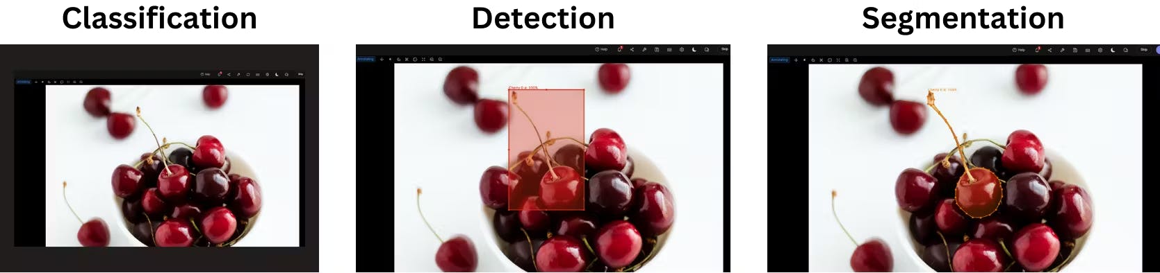
Image Classification vs Object Detection vs Image Segmentation
The ultimate measure of success for contrastive learning is its performance on downstream tasks. The learned representations are input features for tasks such as image classification, object detection, sentiment analysis, or language translation.
The model's performance on these tasks is evaluated using appropriate metrics, including accuracy, precision, recall, F1 score, or task-specific evaluation criteria. Higher performance on the downstream tasks indicates better generalization and usefulness of the learned representations.
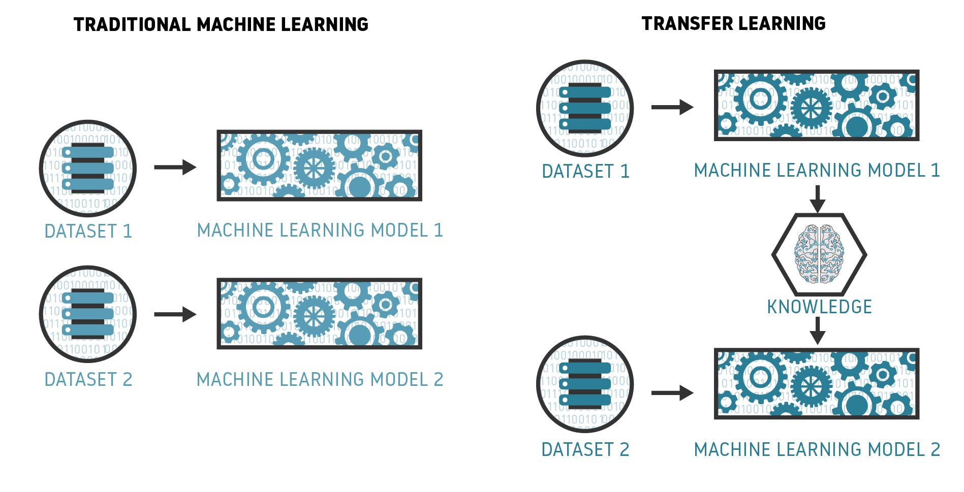
Transfer Learning
Contrastive learning enables transfer learning, where the presentation of learned representations from one task can be applied to related tasks. Generalization is evaluated by assessing how well the representations transfer to new tasks or datasets. If the learned representations generalize well to unseen data and improve performance on new tasks, it indicates the effectiveness of contrastive learning in capturing meaningful features and similarities.
Is Transfer Learning the final step for enabling AI in Aviation?
Comparison with Baselines
To understand the effectiveness of contrastive learning, comparing the learned representations with baseline models or other state-of-the-art approaches is essential. Comparisons can be made regarding performance metrics, robustness, transfer learning capabilities, or computational efficiency. Such comparisons provide insights into the added value of contrastive learning and its potential advantages over alternative methods.
After understanding how contrastive learning works, let's explore an essential aspect of this learning technique: the choice and role of loss functions.
Loss Functions in Contrastive Learning
In contrastive learning, various loss functions are employed to define the objectives of the learning process. These loss functions guide the model in capturing meaningful representations and discriminating between similar and dissimilar instances. By understanding the different loss functions used in contrastive learning, we can gain insights into how they contribute to the learning process and enhance the model's ability to capture relevant features and similarities within the data.
Contrastive Loss
Contrastive loss is a fundamental loss function in contrastive learning. It aims to maximize the agreement between positive pairs (instances from the same sample) and minimize the agreement between negative pairs (instances from different samples) in the learned embedding space. The goal is to pull similar instances closer together while pushing dissimilar instances apart.
The contrastive loss function is typically defined as a margin-based loss, where the similarity between instances is measured using a distance metric, such as Euclidean distance or cosine similarity. The contrastive loss is computed by penalizing positive samples for being far apart and negative samples for being too close in the embedding space.
One widely used variant of contrastive loss is the InfoNCE loss, which we will discuss in more detail shortly. Contrastive loss has shown effectiveness in various domains, including computer vision and natural language processing, as it encourages the model to learn discriminative representations that capture meaningful similarities and differences.
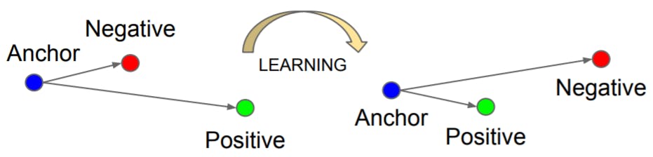
Triplet Loss
Triplet loss is another popular loss function employed in contrastive learning. It aims to preserve the relative distances between instances in the learned representation space. Triplet loss involves forming triplets of instances: an anchor instance, a positive sample (similar to the anchor), and a negative sample (dissimilar to the anchor). The objective is to ensure that the distance between the anchor and the positive sample is smaller than the distance between the anchor and the negative sample by a specified margin.
FaceNet: A Unified Embedding for Face Recognition and Clustering
The intuition behind triplet loss is to create a "triplet constraint" where the anchor instance is pulled closer to the positive sample while being pushed away from the negative sample. The model can better discriminate between similar and dissimilar instances by learning representations that satisfy the triplet constraint.
Triplet loss has been widely applied in computer vision tasks, such as face recognition and image retrieval, where capturing fine-grained similarities is crucial. However, triplet loss can be sensitive to the selection of triplets, as choosing informative triplets from a large dataset can be challenging and computationally expensive.
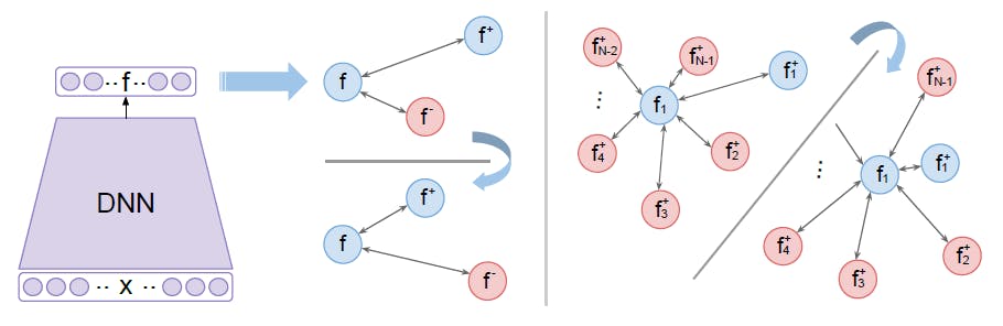
N-pair Loss
N-pair loss is an extension of triplet loss that considers multiple positive and negative samples for a given anchor instance. Rather than comparing an anchor instance to a single positive and negative sample, N-pair loss aims to maximize the similarity between the anchor and all positive instances while minimizing the similarity between the anchor and all negative instances.
Improved Deep Metric Learning with Multi-class N-pair Loss Objective
The N-pair loss encourages the model to capture nuanced relationships among multiple instances, providing more robust supervision during learning. By considering multiple instances simultaneously, N-pair loss can capture more complex patterns and improve the discriminative power of the learned representations.
N-pair loss has been successfully employed in various tasks, such as fine-grained image recognition, where capturing subtle differences among similar instances is essential. It alleviates some of the challenges associated with triplet loss by leveraging multiple positive and negative instances, but it can still be computationally demanding when dealing with large datasets.
InfoNCE
Information Noise Contrastive Estimation (InfoNCE) loss is derived from the framework of noise contrastive estimation. It measures the similarity between positive and negative pairs in the learned embedding space. InfoNCE loss maximizes the agreement between positive pairs and minimizes the agreement between negative pairs.
The key idea behind InfoNCE loss is to treat the contrastive learning problem as a binary classifier. Given a positive pair and a set of negative pairs, the model is trained to discriminate between positive and negative instances. The similarity between instances is measured using a probabilistic approach, such as the softmax function.
InfoNCE loss is commonly used in self-supervised contrastive learning, where positive pairs are created from augmented views of the same instance, and negative pairs are formed using instances from different samples. By optimizing InfoNCE loss, the model learns to capture meaningful similarities and differences in the data points, acquiring powerful representations.
Logistic Loss
Logistic loss, also known as logistic regression loss or cross-entropy loss, is a widely used loss function in machine learning. It has been adapted for contrastive learning as a probabilistic loss function. Logistic loss models the likelihood of two instances being similar or dissimilar based on their respective representations in the embedding space.
Logistic loss is commonly employed in contrastive learning to estimate the probability that two instances belong to the same class (similar) or different classes (dissimilar). By maximizing the likelihood of positive pairs being similar and minimizing the likelihood of negative pairs being similar, logistic loss guides the model toward effective discrimination.
The probabilistic nature of logistic loss makes it suitable for modeling complex relationships and capturing fine-grained differences between instances. Logistic loss has been successfully applied in various domains, including image recognition, text classification, and recommendation systems.
These different loss functions provide diverse ways to optimize the contrastive learning objective and encourage the model to learn representations that capture meaningful similarities and differences in the data points. The choice of loss function depends on the specific requirements of the task and the characteristics of the data.
By leveraging these objectives, contrastive learning enables models to learn powerful representations that facilitate better discrimination and generalization in various machine learning applications.
Contrastive Learning: Use Cases
Let's explore some prominent use cases where contrastive learning has proven to be effective:
Semi-Supervised Learning
Semi-supervised learning is a scenario where models are trained using labeled and unlabeled data. Obtaining labeled data can be costly and time-consuming in many real-world situations, while unlabeled data is abundant. Contrastive learning is particularly beneficial in semi-supervised learning as it allows models to leverage unlabeled data to learn meaningful representations.
By training on unlabeled data using contrastive learning, models can capture useful patterns and improve performance when labeled data is limited. Contrastive learning enables the model to learn discriminative representations that capture relevant features and similarities in the data. These learned representations can then enhance performance on downstream tasks, such as image classification, object recognition, speech recognition, and more.
Supervised Learning
Contrastive learning also has applications in traditional supervised learning scenarios with plentiful labeled data. In supervised learning, models are trained on labeled data to predict or classify new instances. However, labeled data may not always capture the full diversity and complexity of real-world instances, leading to challenges in generalization.
By leveraging unlabeled data alongside labeled data, contrastive learning can augment the learning process and improve the discriminative power of the model. The unlabeled data provides additional information and allows the model to capture more robust representations. This improves performance on various supervised learning tasks, such as image classification, sentiment analysis, recommendation systems, and more.
NLP
Contrastive learning has shown promising results in natural language processing (NLP). NLP deals with the processing and understanding human language, and contrastive learning has been applied to enhance various NLP tasks.
Contrastive learning enables models to capture semantic information and contextual relationships by learning representations from large amounts of unlabeled text data. This has been applied to tasks such as sentence similarity, text classification, language modeling, sentiment analysis, machine translation, and more.
For example, in sentence similarity tasks, contrastive learning allows models to learn representations that capture the semantic similarity between pairs of sentences. By leveraging the power of contrastive learning, models can better understand the meaning and context of sentences, facilitating more accurate and meaningful comparisons.
Data Augmentation
Augmentation involves applying various transformations or perturbations to unlabeled data to create diverse instances or augmented views. These augmented views serve as positive pairs during the contrastive learning, allowing the model to learn robust representations that capture relevant features.
Data augmentation techniques used in contrastive learning include cropping, flipping, rotation, color transformations, and more. By generating diverse instances, contrastive learning ensures that the model learns to capture relevant information regardless of variations in the input data.
Data augmentation plays a crucial role in combating data scarcity and addressing the limitations of labeled data. By effectively utilizing unlabeled data through contrastive learning and data augmentation, models can learn more generalized and robust representations, improving performance on various tasks, especially in computer vision domains.
Popular Contrastive Learning Frameworks
In recent years, several contrastive learning frameworks have gained prominence in deep learning due to their effectiveness in learning powerful representations. Let’s explore some popular contrastive learning frameworks that have garnered attention:
SimCLR
Simple Contrastive Learning of Representations (SimCLR) is a self-supervised contrastive learning framework that has garnered widespread recognition for its effectiveness in learning powerful representations. It builds upon the principles of contrastive learning by leveraging a combination of data augmentation, a carefully designed contrastive objective, and a symmetric neural network architecture.

Advancing Self-Supervised and Semi-Supervised Learning with SimCLR
The core idea of SimCLR is to maximize the agreement between augmented views of the same instance while minimizing the agreement between views from different instances. By doing so, SimCLR encourages the model to learn representations that capture meaningful similarities and differences in the data. The framework employs a large-batch training scheme to facilitate efficient and effective contrastive learning.
Additionally, SimCLR incorporates a specific normalization technique called "normalized temperature-scaled cross-entropy" (NT-Xent) loss, which enhances training stability and improves the quality of the learned representations.
SimCLR has demonstrated remarkable performance across various domains, including computer vision, natural language processing, and reinforcement learning. It outperforms prior methods in several benchmark datasets and tasks, showcasing its effectiveness in learning powerful representations without relying on explicit labels.
MoCo
Momentum Contrast (MoCo) is another prominent self-supervised contrastive learning framework that has garnered significant attention. It introduces the concept of a dynamic dictionary of negative instances, which helps the model capture meaningful features and similarities in the data. MoCo utilizes a momentum encoder, which gradually updates the representations of negative examples to enhance the model's ability to capture relevant information.
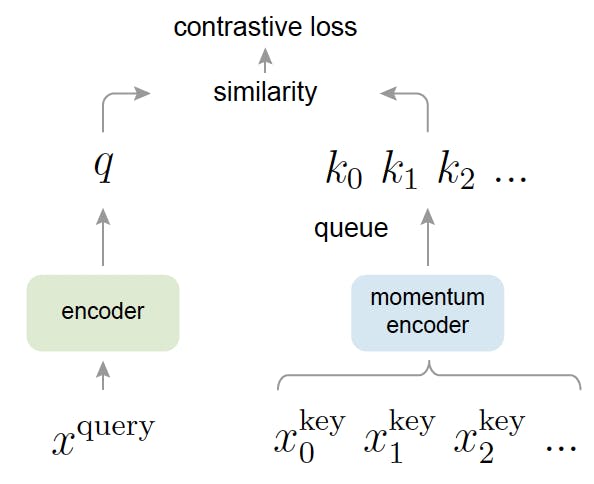
Momentum Contrast for Unsupervised Visual Representation Learning
The framework maximizes agreement between positive pairs while minimizing agreement between negative pairs. By maintaining a dynamic dictionary of negative instances, MoCo provides richer contrasting examples for learning representations. It has shown strong performance in various domains, including computer vision and natural language processing, and has achieved state-of-the-art results in multiple benchmark datasets.
BYOL
Bootstrap Your Own Latent (BLOY) is a self-supervised contrastive learning framework that emphasizes the online updating of target network parameters. It employs a pair of online and target networks, with the target network updated through exponential moving averages of the online network's weights. BYOL focuses on learning representations without the need for negative examples.
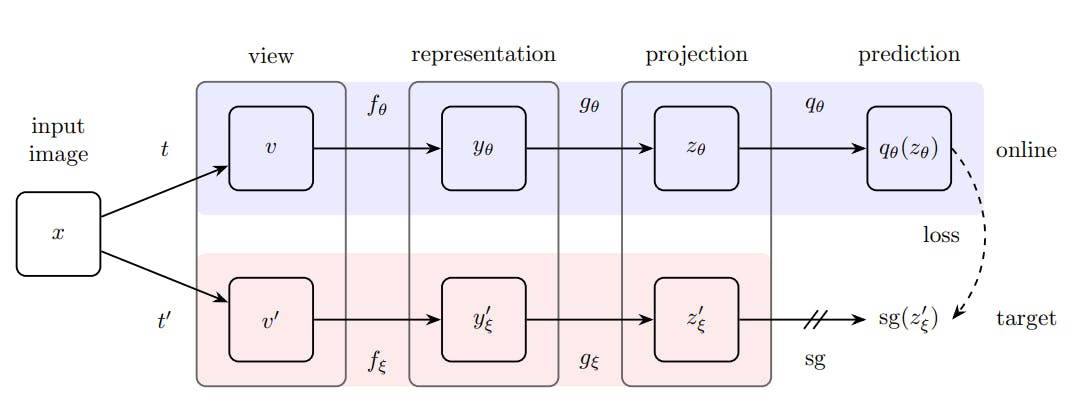
Bootstrap your own latent: A new approach to self-supervised Learning
The framework maximizes agreement between augmented views of the same instance while decoupling the similarity estimation from negative examples. BYOL has demonstrated impressive performance in various domains, including computer vision and natural language processing. It has shown significant gains in representation quality and achieved state-of-the-art results in multiple benchmark datasets.
SwAV
Swapped Augmentations and Views (SwAV) is a self-supervised contrastive learning framework that introduces clustering-based objectives to learn representations. It leverages multiple augmentations of the same image and multiple views within a mini-batch to encourage the model to assign similar representations to augmented views of the same instance.
Using clustering objectives, SwAV aims to identify clusters of similar representations without the need for explicit class labels. It has shown promising results in various computer vision tasks, including image classification and object detection, and has achieved competitive performance on several benchmark datasets.
Barlow Twins
Barlow Twins is a self-supervised contrastive learning framework that reduces cross-correlation between latent representations. It introduces a decorrelation loss that explicitly encourages the model to produce diverse representations for similar instances, enhancing the overall discriminative power.
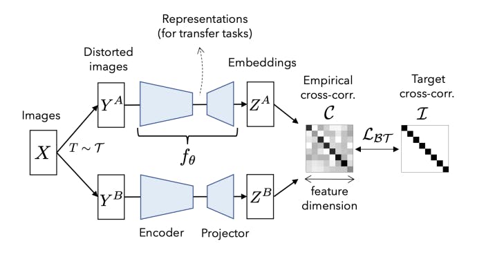
Barlow Twins: Self-Supervised Learning via Redundancy Reduction
Barlow Twins aims to capture more unique and informative features in the learned representations by reducing cross-correlation. The framework has demonstrated impressive performance in various domains, including computer vision and natural language processing, and has achieved state-of-the-art results in multiple benchmark datasets.
By leveraging the principles of contrastive learning and incorporating innovative methodologies, these frameworks have paved the way for advancements in various domains, including computer vision, natural language processing, and reinforcement learning.
Contrastive Learning: Key Takeaways
- Contrastive learning is a powerful technique for learning meaningful representations from unlabeled data, leveraging similarity and dissimilarity to map instances in a latent space.
- It encompasses supervised contrastive learning (SSCL) with labeled data and self-supervised contrastive learning (SCL) with pretext tasks for unlabeled data.
- Important components include data augmentation, encoder, and projection networks, capturing relevant features and similarities.
- Common loss functions used in contrastive learning are contrastive loss, triplet loss, N-pair loss, InfoNCE loss, and logistic loss.
- Contrastive learning has diverse applications, such as semi-supervised learning, supervised learning, NLP, and data augmentation, and it improves model performance and generalization.

Power your AI models with the right data
Automate your data curation, annotation and label validation workflows.
Get startedWritten by

Nikolaj Buhl
- Contrastive learning is a machine learning technique that aims to learn meaningful representations by contrasting positive and negative pairs of instances. It leverages the assumption that similar instances should be closer together in a learned embedding space, while dissimilar instances should be farther apart.
- Contrastive learning differs from traditional supervised learning in that it doesn’t rely on explicit labels for training. Instead, it learns representations by contrasting positive and negative pairs of data points. This makescontrastive learning suitable for scenarios where labeled data is limited or unavailable.
- Contrastive learning can be applied to various types of data, including images, text, audio, and other types of structured and unstructured data. As long as there are meaningful similarities and dissimilarities between instances, contrastive learning can be used to learn representations from the data.
- Contrastive learning can be beneficial for small datasets because it leverages unlabeled data to enhance representation learning. By learning from a combination of labeled and unlabeled data, contrastive learning can help improve the model's generalization and performance on small datasets.
- Yes, contrastive learning can be combined with other learning techniques to further enhance representation learning. For example, contrastive learning can be used in conjunction with transfer learning, where pre-trained representations from one task or domain are fine-tuned on a target task. This combination allows leveraging the benefits of both techniques for improved performance.
Related blogs


Visualizations in Databricks
With data becoming a pillar stone of a company’s growth strategy, the market for visualization tools is growing rapidly, with a projected compound annual growth rate (CAGR) of 10.07% between 2023 and 2028. The primary driver of these trends is the need for data-driven decision-making, which involves understanding complex data patterns and extracting actionable insights to improve operational efficiency. PowerBI and Tableau are traditional tools with interactive workspaces for creating intuitive dashboards and exploring large datasets. However, other platforms are emerging to address the ever-changing nature of the modern data ecosystem. In this article, we will discuss the visualizations offered by Databricks - a modern enterprise-scale platform for building data, analytics, and artificial intelligence (AI) solutions. Databricks Databricks is an end-to-end data management and model development solution built on Apache Spark. It lets you create and deploy the latest generative AI (Gen AI) and large language models (LLMs). The platform uses a proprietary Mosaic AI framework to streamline the model development process. It provides tools to fine-tune LLMs seamlessly through enterprise data and offers a unified service for experimentation through foundation models. In addition, it features Databricks SQL, a state-of-the-art lakehouse for cost-effective data storage and retrieval. It lets you centrally store all your data assets in an open format, Delta Lake, for effective governance and discoverability. Further, Databricks SQL has built-in support for data visualization, which lets you extract insights from datasets directly from query results in the SQL editor. Users also benefit from the visualization tools featured in Databricks Notebooks, which help you build interactive charts by using the Plotly library in Python. Through these visualizations, Databricks offers robust data analysis for monitoring data assets critical to your AI models. So, let’s discuss in more detail the types of chart visualizations, graphs, diagrams, and maps available on Databricks to help you choose the most suitable visualization type for your use case. Effective visualization can help with effortless data curation. Learn more about how you can use data curation for computer vision Visualizations in Databricks As mentioned earlier, Databricks provides visualizations through Databricks SQL and Databricks Notebooks. The platform lets you run multiple SQL queries to perform relevant aggregations and apply filters to visualize datasets according to your needs. Databricks also allows you to configure settings related to the X and Y axes, legends, missing values, colors, and labels. Users can also download visualizations in PNG format for documentation purposes. The following sections provide an overview of the various visualization types available in these two frameworks, helping you select the most suitable option for your project. Bar Chart Bar charts are helpful when you want to compare the frequency of occurrence of different categories in your dataset. For instance, you can draw a bar chart to compare the frequency of various age groups, genders, ethnicities, etc. Additionally, bar charts can be used to view the sum of the prices of all orders placed in a particular month and group them by priority. Bar chart The result will show the months on the X-axis and the sum of all the orders categorized by priority on the Y-axis. Line Line charts connect different data points through straight lines. They are helpful when users want to analyze trends over some time. The charts usually show time on the X-axis and some metrics whose trajectory you want to explore on the Y-axis. Line chart For instance, you can view changes in the average price of orders over the years grouped by priority. The trends can help you predict the most likely future values, which can help you with financial projections and budget planning. Pie Chart Pie charts display the proportion of different categories in a dataset. They divide a circle into multiple segments, each showing the proportion of a particular category, with the segment size proportional to the category’s percentage of the total. Pie chart For instance, you can visualize the proportion of orders for each priority. The visualization is helpful when you want a quick overview of data distribution across different segments. It can help you analyze demographic patterns, market share of other products, budget allocation, etc. Scatter Plot A scatter plot displays each data point as a dot representing a relationship between two variables. Users can also control the color of each dot to reflect the relationship across different groups. Scatter Plot For instance, you can plot the relationship between quantity and price for different color-coded item categories. The visualization helps in understanding the correlation between two variables. However, users must interpret the relationship cautiously, as correlation does not always imply causation. Deeper statistical analysis is necessary to uncover causal factors. Area Charts Area charts combine line and bar charts by displaying lines and filling the area underneath with colors representing particular categories. They show how the contribution of a specific category changes relative to others over time. Area Charts For instance, you can visualize which type of order priority contributed the most to revenue by plotting the total price of different order priorities across time. The visualization helps you analyze the composition of a specific metric and how that composition varies over time. It is particularly beneficial in analyzing sales growth patterns for different products, as you can see which product contributed the most to growth across time. Box Chart Box charts concisely represent data distributions of numerical values for different categories. They show the distribution’s median, skewness, interquartile, and value ranges. Box Chart For instance, the box can display the median price value through a line inside the box and the interquartile range through the top and bottom box enclosures. The extended lines represent minimum and maximum price values to compute the price range. The chart helps determine the differences in distribution across multiple categories and lets you detect outliers. You can also see the variability in values across different categories and examine which category was the most stable. Bubble Chart Bubble charts enhance scatter plots by allowing you to visualize the relationship of three variables in a two-dimensional grid. The bubble position represents how the variable on the X-axis relates to the variable on the Y-axis. The bubble size represents the magnitude of a third variable, showing how it changes as the values of the first two variables change. Bubble chart The visualization is helpful for multi-dimensional datasets and provides greater insight when analyzing demographic data. However, like scatter plots, users must not mistake correlation for causation. Combo Chart Combo charts combine line and bar charts to represent key trends in continuous and categorical variables. The categorical variable is on the X-axis, while the continuous variable is on the Y-axis. Combo Chart For instance, you can analyze how the average price varies with the average quantity according to shipping date. The visualization helps summarize complex information involving relationships between three variables on a two-dimensional graph. However, unambiguous interpretation requires careful configuration of labels, colors, and legends. Heatmap Chart Heatmap charts represent data in a matrix format, with each cell having a different color according to the numerical value of a specific variable. The colors change according to the value intensity, with lower values typically having darker and higher values having lighter colors. Heatmap chart For instance, you can visualize how the average price varies according to order priority and order status. Heatmaps are particularly useful in analyzing correlation intensity between two variables. They also help detect outliers by representing unusual values through separate colors. However, interpreting the chart requires proper scaling to ensure colors do not misrepresent intensities. Histogram Histograms display the frequency of particular value ranges to show data distribution patterns. The X-axis contains the value ranges organized as bins, and the Y-axis shows the frequency of each bin. Histogram For instance, you can visualize the frequency of different price ranges to understand price distribution for your orders. The visualization lets you analyze data spread and skewness. It is beneficial in deeper statistical analysis, where you want to derive probabilities and build predictive models. Pivot Tables Pivot tables can help you manipulate tabular displays through drag-and-drop options by changing aggregation records. The option is an alternative to SQL filters for viewing aggregate values according to different conditions. Pivot Tables For instance, you can group total orders by shipping mode and order category. The visualization helps prepare ad-hoc reports and provides important summary information for decision-making. Interactive pivot tables also let users try different arrangements to reveal new insights. Choropleth Map Visualization Choropleth map visualization represents color-coded aggregations categorized according to different geographic locations. Regions with higher value intensities have darker colors, while those with lower intensities have lighter shades. Choropleth map visualization For instance, you can visualize the total revenue coming from different countries. This visualization helps determine global presence and highlight disparities across borders. The insights will allow you to develop marketing strategies tailored to regional tastes and behavior. Funnel Visualization Funnel visualization depicts data aggregations categorized according to specific steps in a pipeline. It represents each step from top to bottom with a bar and the associated value as a label overlay on each bar. It also displays cumulative percentage values showing the proportion of the aggregated value resulting from each stage. Funnel Visualization For instance, you can determine the incoming revenue streams at each stage of the ordering process. This visualization is particularly helpful in analyzing marketing pipelines for e-commerce sites. The tool shows the proportion of customers who view a product ad, click on it, add it to the cart, and proceed to check out. Cohort Analysis Cohort analysis offers an intuitive visualization to track the trajectory of a particular metric across different categories or cohorts. Cohort Analysis For instance, you can analyze the number of active users on an app that signed up in different months of the year. The rows will depict the months, and the columns will represent the proportion of active users in a particular cohort as they move along each month. The visualization helps in retention analysis as you can determine the proportion of retained customers across the user lifecycle. Counter Display Databricks allows you to configure a counter display that explicitly shows how the current value of a particular metric compares with the metric’s target value. Counter display For instance, you can check how the average total revenue compares against the target value. In Databricks, the first row represents the current value, and the second is the target. The visualization helps give a quick snapshot of trending performance and allows you to quantify goals for better strategizing. Sankey Diagrams Sankey diagrams show how data flows between different entities or categories. It represents flows through connected links representing the direction, with entities displayed as nodes on either side of a two-dimensional grid. The width of the connected links represents the magnitude of a particular value flowing from one entity to the other. Sankey Diagram For instance, you can analyze traffic flows from one location to the other. Sankey diagrams can help data engineering teams analyze data flows from different platforms or servers. The analysis can help identify bottlenecks, redundancies, and resource constraints for optimization planning. Sunburst Sequence The sunburst sequence visualizes hierarchical data through concentric circles. Each circle represents a level in the hierarchy and has multiple segments. Each segment represents the proportion of data in the hierarchy. Furthermore, it color codes segments to distinguish between categories within a particular hierarchy. Sunburst Sequence For instance, you can visualize the population of different world regions through a sunburst sequence. The innermost circle represents a continent, the middle one shows a particular region, and the outermost circle displays the country within that region. The visualization helps data science teams analyze relationships between nested data structures. The information will allow you to define clear data labels needed for model training. Table A table represents data in a structured format with rows and columns. Databricks offers additional functionality to hide, reformat, and reorder data. Tables help summarize information in structured datasets. You can use them for further analysis through SQL queries. Word Cloud Word cloud visualizations display words in different sizes according to their frequency in textual data. For instance, you can analyze customer comments or feedback and determine overall sentiment based on the highest-occurring words. Word Cloud While word clouds help identify key themes in unstructured textual datasets, they can suffer from oversimplification. Users must use word clouds only as a quick overview and augment textual analysis with advanced natural language processing techniques. Visualization is critical to efficient data management. Find out the top tools for data management for computer vision Visualizations in Databricks: Key Takeaways With an ever-increasing data volume and variety, visualization is becoming critical for quickly communicating data-based insights in a simplified manner. Databricks is a powerful tool with robust visualization types for analyzing complex datasets. Below are a few key points to remember regarding visualization in Databricks. Databricks SQL and Databricks Notebooks: Databricks offers advanced visualizations through Databricks SQL and Databricks Notebooks as a built-in functionality. Visualization configurations: Users can configure multiple visualization settings to produce charts, graphs, maps, and diagrams per their requirements. Visualization types: Databricks offers multiple visualizations, including bar charts, line graphs, pie charts, scatter plots, area graphs, box plots, bubble charts, combo charts, heatmaps, histograms, pivot tables, choropleth maps, funnels, cohort tables, counter display, Sankey diagrams, sunburst sequences, tables, and word clouds.
Mar 28 2024
10 M


Microsoft MORA: Multi-Agent Video Generation Framework
What is Mora? Mora is a multi-agent framework designed for generalist video generation. Based on OpenAI's Sora, it aims to replicate and expand the range of generalist video generation tasks. Sora, famous for making very realistic and creative scenes from written instructions, set a new standard for creating videos that are up to a minute long and closely match the text descriptions given. Mora distinguishes itself by incorporating several advanced visual AI agents into a cohesive system. This lets it undertake various video generation tasks, including text-to-video generation, text-conditional image-to-video generation, extending generated videos, video-to-video editing, connecting videos, and simulating digital worlds. Mora can mimic Sora’s capabilities using multiple visual agents, significantly contributing to video generation. In this article, you will learn: Mora's innovative multi-agent framework for video generation. The importance of open-source collaboration that Mora enables. Mora's approach to complex video generation tasks and instruction fidelity. About the challenges in video dataset curation and quality enhancement. TL; DR Mora's novel approach uses multiple specialized AI agents, each handling different aspects of the video generation process. This innovation allows various video generation tasks, showcasing adaptability in creating detailed and dynamic video content from textual descriptions. Mora aims to fix the problems with current models like Sora, which is closed-source and does not let anyone else use it or do more research in the field, even though it has amazing text-to-video conversion abilities 📝🎬. Unfortunately, Mora still has problems with dataset quality, video fidelity, and ensuring that outputs align with complicated instructions and people's preferences. These problems show where more work needs to be done in the future. OpenAI Sora’s Closed-Source Nature The closed-source nature of OpenAI's Sora presents a significant challenge to the academic and research communities interested in video generation technologies. Sora's impressive capabilities in generating realistic and detailed videos from text descriptions have set a new standard in the field. Related: New to Sora? Check out our detailed explainer on the architecture, relevance, limitations, and applications of Sora. However, the inability to access its source code or detailed architecture hinders external efforts to replicate or extend its functionalities. This limits researchers from fully understanding or replicating its state-of-the-art performance in video generation. Here are the key challenges highlighted due to Sora's closed-source nature: Inaccessibility to Reverse-Engineer Without access to Sora's source code, algorithms, and detailed methodology, the research community faces substantial obstacles in dissecting and understanding the underlying mechanisms that drive its exceptional performance. This lack of transparency makes it difficult for other researchers to learn from and build upon Sora's advancements, potentially slowing down the pace of innovation in video generation. Extensive Training Datasets Sora's performance is not just the result of sophisticated modeling and algorithms; it also benefits from training on extensive and diverse datasets. But the fact that researchers cannot get their hands on similar datasets makes it very hard to copy or improve Sora's work. High-quality, large-scale video datasets are crucial for training generative models, especially those capable of creating detailed, realistic videos from text descriptions. However, these datasets are often difficult to compile due to copyright issues, the sheer volume of data required, and the need for diverse, representative samples of the real world. Creating, curating, and maintaining high-quality video datasets requires significant resources, including copyright permissions, data storage, and management capabilities. Sora's closed nature worsens these challenges by not providing insights into compiling the datasets, leaving researchers to navigate these obstacles independently. Computational Power Creating and training models like Sora require significant computational resources, often involving large clusters of high-end GPUs or TPUs running for extended periods. Many researchers and institutions cannot afford this much computing power, which makes the gap between open-source projects like Mora and proprietary models like Sora even bigger. Without comparable computational resources, it becomes challenging to undertake the necessary experimentation—with different architectures and hyperparameters—and training regimes required to achieve similar breakthroughs in video generation technology. Learn more about these limitations in the technical paper. Evolution: Text-to-Video Generation Over the years, significant advancements in text-to-video generation technology have occurred, with each approach and architecture uniquely contributing to the field's growth. Here's a summary of these evolutionary stages, as highlighted in the discussion about text-to-video generation in the Mora paper: GANs (Generative Adversarial Networks) Early attempts at video generation leveraged GANs, which consist of two competing networks: a generator that creates images or videos that aim to be indistinguishable from real ones, and a discriminator that tries to differentiate between the real and generated outputs. Despite their success in image generation, GANs faced challenges in video generation due to the added complexity of temporal coherence and higher-dimensional data. Generative Video Models Moving beyond GANs, the field saw the development of generative video models designed to produce dynamic sequences. Generating realistic videos frame-by-frame and maintaining temporal consistency is a challenge, unlike in static image generation. Auto-Regressive Transformers Auto-regressive transformers were a big step forward because they could generate video sequences frame-by-frame. These models predicted each new frame based on the previously generated frames, introducing a sequential element that mirrors the temporal progression of videos. But this approach often struggled with long-term coherence over longer sequences. Large-Scale Diffusion Models Diffusion models, known for their capacity to generate high-quality images, were extended to video generation. These models gradually refine a random noise distribution toward a coherent output. They apply this iterative denoising process to the temporal domain of videos. Related: Read our guide on HuggingFace’s Dual-Stream Diffusion Net for Text-to-Video Generation. Image Diffusion U-Net Adapting the U-Net architecture for image diffusion models to video content was critical. This approach extended the principles of image generation to videos, using a U-Net that operates over sequences of frames to maintain spatial and temporal coherence. 3D U-Net Structure The change to a 3D U-Net structure allowed for more nuance in handling video data, considering the extra temporal dimension. This change also made it easier to model time-dependent changes, improving how we generate coherent and dynamic video content. Latent Diffusion Models (LDMs) LDMs generate content in a latent space rather than directly in pixel space. This approach reduces computational costs and allows for more efficient handling of high-dimensional video data. LDMs have shown that they can better capture the complex dynamics of video content. Diffusion Transformers Diffusion transformers (DiT) combine the strengths of transformers in handling sequential data with the generative capabilities of diffusion models. This results in high-quality video outputs that are visually compelling and temporally consistent. Useful: Stable Diffusion 3 is an example of a multimodal diffusion transformer model that generates high-quality images and videos from text. Check out our explainer on how it works. AI Agents: Advanced Collaborative Multi-agent Structures The paper highlights the critical role of collaborative, multi-agent structures in developing Mora. It emphasizes their efficacy in handling multimodal tasks and improving video generation capabilities. Here's a concise overview based on the paper's discussion on AI Agents and their collaborative frameworks: Multimodal Tasks Advanced collaborative multi-agent structures address multimodal tasks involving processing and generating complex data across different modes, such as text, images, and videos. These structures help integrate various AI agents, each specialized in handling specific aspects of the video generation process, from understanding textual prompts to creating visually coherent sequences. Cooperative Agent Framework (Role-Playing) The cooperative agent framework, characterized by role-playing, is central to the operation of these multi-agent structures. Each agent is assigned a unique role or function in this framework, such as prompt enhancement, image generation, or video editing. By defining these roles, the framework ensures that an agent with the best skills for each task is in charge of that step in the video generation process, increasing overall efficiency and output quality. Multi-Agent Collaboration Strategy The multi-agent collaboration strategy emphasizes the orchestrated interaction between agents to achieve a common goal. In Mora, this strategy involves the sequential and sometimes parallel processing of tasks by various agents. For instance, one agent might enhance an initial text prompt, convert it into another image, and finally transform it into a video sequence by yet another. This collaborative approach allows for the flexible and dynamic generation of video content that aligns with user prompts. AutoGen (Generic Programming Framework) A notable example of multi-agent collaboration in practice is AutoGen. This generic programming framework is designed to automate the assembly and coordination of multiple AI agents for a wide range of applications. Within the context of video generation, AutoGen can streamline the configuration of agents according to the specific requirements of each video generation task to generate complex video content from textual or image-based prompts. Mora drone to butterfly flythrough shot. | Image Source. Role of an AI Agent The paper outlines the architecture involving multiple AI agents, each serving a specific role in the video generation process. Here's a closer look at the role of each AI agent within the framework: Illustration of how to use Mora to conduct video-related tasks Prompt Selection and Generation Agent This agent is tasked with processing and optimizing textual prompts for other agents to process them further. Here are the key techniques used for Mora: GPT-4: This agent uses the generative capabilities of GPT-4 to generate high-quality prompts that are detailed and rich in context. Prompt Selection: This involves selecting or enhancing textual prompts to ensure they are optimally prepared for the subsequent video generation process. This step is crucial for setting the stage for generating images and videos that closely align with the user's intent. Good Read: Interested in GPT-4 Vision alternatives? Check out our blog post. Text-to-Image Generation Agent This agent uses a retrained large text-to-image model to convert the prompts into initial images. The retraining process ensures the model is finely tuned to produce high-quality images, laying a strong foundation for the video generation process. Image-to-Image Generation Agent This agent specializes in image-to-image generation, taking initial images and editing them based on new prompts or instructions. This ability allows for a high degree of customization and improvement in video creation. Image-to-Video Generation Agent This agent transforms static images into dynamic video sequences, extending the visual narrative by generating coherent frames. Here are the core techniques and models: Core Components: It incorporates two pre-trained models: GPT-3 for understanding and generating text-based instructions, and Stable Diffusion for translating these instructions into visual content. Prompt-to-Prompt Technique: The prompt-to-prompt technique guides the transformation from an initial image to a series of images that form a video sequence. Classifier-Free Guidance: Classifier-free guidance is used to improve the fidelity of generated videos to the textual prompts so that the videos remain true to the users' vision. Text-to-Video Generation Agent: This role is pivotal in transforming static images into dynamic videos that capture the essence of the provided descriptions. Stable Video Diffusion (SVD) and Hierarchical Training Strategy: A model specifically trained to understand and generate video content, using a hierarchical training strategy to improve the quality and coherence of the generated videos. Video Connection Agent This agent creates seamless transitions between two distinct video sequences for a coherent narrative flow. Here are the key techniques used: Pre-Trained Diffusion-Based T2V Model: This model uses a pre-trained diffusion-based model specialized in text-to-video (T2V) tasks to connect separate video clips into a cohesive narrative. Text-Based Control: This method uses textual descriptions to guide the generation of transition videos that seamlessly connect disparate video clips, ensuring logical progression and thematic consistency. Image-to-Video Animation and Autoregressive Video Prediction: These capabilities allow the agent to animate still images into video sequences, predict and generate future video frames based on previous sequences, and create extended and coherent video narratives. Mora’s Video Generation Process Mora's video-generation method is a complex, multi-step process that uses the unique capabilities of specialized AI agents within its framework. This process allows Mora to tackle various video generation tasks, from creating videos from text descriptions to editing and connecting existing videos. Here's an overview of how Mora handles each task: Mora’s video generation process. Text-to-Video Generation This task begins with a detailed textual prompt from the user. Then, the Text-to-Image Generation Agent converts the prompts into initial static images. These images serve as the basis for the Image-to-Video Generation Agent, which creates dynamic sequences that encapsulate the essence of the original text and produce a coherent video narrative. Text-Conditional Image-to-Video Generation This task combines textual prompts with a specific starting image. Mora first improves the input with the Prompt Selection and Generation Agent, ensuring that the text and image are optimally prepared for video generation. Then, the Image-to-Video Generation Agent takes over, generating a video that evolves from the initial image and aligns with the textual description. Extend Generated Videos To extend an existing video, Mora uses the final frame of the input video as a launchpad. The Image-to-Video Generation Agent crafts additional sequences that logically continue the narrative from the last frame, extending the video while maintaining narrative and visual continuity. Video-to-Video Editing In this task, Mora edits existing videos based on new textual prompts. The Image-to-Image Generation Agent first edits the video's initial frame according to the new instructions. Then, the Image-to-Video Generation Agent generates a new video sequence from the edited frame, adding the desired changes to the video content. Connect Videos Connecting two videos involves creating a transition between them. Mora uses the Video Connection Agent, which analyzes the first video's final frame and the second's initial frame. It then generates a transition video that smoothly links the two segments into a cohesive narrative flow. Simulating Digital Worlds Mora generates video sequences in this task that simulate digital or virtual environments. The process involves appending specific style cues (e.g., "in digital world style") to the textual prompt, guiding the Image-to-Video Generation Agent to create a sequence reflecting the aesthetics of a digital realm. This can involve stylistically transforming real-world images into digital representations or generating new content within the specified digital style. See Also: Read our explainer on Google’s Video Gaming Companion: Scalable Instructable Multiworld Agent [SIMA]. Mora: Experimental Setup As detailed in the paper, the experimental setup for evaluating Mora is comprehensive and methodically designed to assess the framework's performance across various dimensions of video generation. Here's a breakdown of the setup: Baseline The baseline for comparison includes existing open-sourced models that showcase competitive performance in video generation tasks. These models include Videocrafter, Show-1, Pika, Gen-2, ModelScope, LaVie-Interpolation, LaVie, and CogVideo. These models are a reference point for evaluating Mora's advancements and position relative to the current state-of-the-art video generation. Basic Metrics The evaluation framework comprises several metrics to quantify Mora's performance across different dimensions of video quality and condition consistency: Video Quality Measurement Object Consistency: Measures the stability of object appearances across video frames. Background Consistency: Assesses the uniformity of the background throughout the video. Motion Smoothness: Evaluates the fluidity of motion within the video. Aesthetic Score: Gauges the artistic and visual appeal of the video. Dynamic Degree: Quantifies the video's dynamic action or movement level. Imaging Quality: Assesses the overall visual quality of the video, including clarity and resolution. Video Condition Consistency Metric Temporal Style: Measures how consistently the video reflects the temporal aspects (e.g., pacing, progression) described in the textual prompt. Appearance Style: Evaluates the adherence of the video's visual style to the descriptions provided in the prompt, ensuring that the generated content matches the intended appearance. Self-Defined Metrics Video-Text Integration (VideoTI): Measures the model’s fidelity to textual instructions by comparing text representations of input images and generated videos. Temporal Consistency (TCON): Evaluates the coherence between an original video and its extended version, providing a metric for assessing the integrity of extended video content. Temporal Coherence (Tmean): Quantifies the correlation between the intermediate generated and input videos, measuring overall temporal coherence. Video Length: This parameter quantifies the duration of the generated video content, indicating the model's capacity for producing videos of varying lengths. Implementation Details The experiments use high-performance hardware, specifically TESLA A100 GPUs with substantial VRAM. This setup ensures that Mora and the baseline models are evaluated under conditions allowing them to fully express their video generation capabilities. The choice of hardware reflects the computational intensity of training and evaluating state-of-the-art video generation models. Mora video generation - Fish underwater flythrough Limitations of Mora The paper outlines several limitations of the Mora framework. Here's a summary of these key points: Curating High-Quality Video Datasets Access to high-quality video datasets is a major challenge for training advanced video generation models like Mora. Copyright restrictions and the sheer volume of data required make it difficult to curate diverse and representative datasets that can train models capable of generating realistic and varied video content. Read Also: The Full Guide to Video Annotation for Computer Vision. Quality and Length Gaps While Mora demonstrates impressive capabilities, it has a noticeable gap in quality and maximum video length compared to state-of-the-art models like Sora. This limitation is particularly evident in tasks requiring the generation of longer videos, where maintaining visual quality and coherence becomes increasingly challenging. Simulating videos in Mora vs in Sora. Instruction Following Capability Mora sometimes struggles to precisely follow complex or detailed instructions, especially when generating videos that require specific actions, movements, or directionality. This limitation suggests that further improvement in understanding and interpreting textual prompts is needed. Human Visual Preference Alignment The experimental results may not always align with human visual preferences, particularly in scenarios requiring the generation of realistic human movements or the seamless connection of video segments. This misalignment highlights the need to incorporate a more nuanced understanding of physical laws and human dynamics into the video-generation process. Mora Vs. Sora: Feature Comparisons The paper compares Mora and OpenAI's Sora across various video generation tasks. Here's a detailed feature comparison based on their capabilities in different aspects of video generation: Check out the project repository on GitHub. Mora Multi-Agent Framework: Key Takeaways The paper "Mora: Enabling Generalist Video Generation via a Multi-Agent Framework" describes Mora, a new framework that advances video technology. Using a multi-agent approach, Mora is flexible and adaptable across various video generation tasks, from creating detailed scenes to simulating complex digital worlds. Because it is open source, it encourages collaboration, which leads to new ideas, and lets the wider research community add to and improve its features. Even though Mora has some good qualities, it needs high-quality video datasets, video quality, length gaps, trouble following complicated instructions correctly, and trouble matching outputs to how people like to see things. Finding solutions to these problems is necessary to make Mora work better and be used in more situations. Continuing to improve and develop Mora could change how we make video content so it is easier for creators and viewers to access and have an impact.
Mar 26 2024
8 M


Panoptic Segmentation Updates in Encord
Panoptic Segmentation Updates in Encord Over the past 6 months, we have updated and built new features within Encord with a strong focus on improving your panoptic segmentation workflows across data, labeling, and model evaluation. Here are some updates we’ll cover in this article: Bitmask lock. SAM + Bitmask lock + Brush for AI-assisted precision labeling. Fast and performant rendering of fully bitmask-segmented images and videos. Panoptic Quality model evaluation metrics. Bitmask Lock within Encord Annotate to Manage Segmentation Overlap Our Bitmask Lock feature introduces a way to prevent segmentation and masks from overlapping, providing pixel-perfect accuracy for your object segmentation tasks. By simply toggling the “Bitmask cannot be drawn over” button, you can prevent any part of a bitmask label from being included in another label. This feature is crucial for applications requiring precise object boundaries and pixel-perfect annotations, eliminating the risk of overlapping segmentations. Let’s see how to do this within Encord Annotate: Step 1: Create your first Bitmask Initiating your labeling process with the Bitmask is essential for creating precise object boundaries. If you are new to the Bitmask option, check out our quickstart video walkthrough on creating your first Bitmask using brush tools for labeling. Step 2: Set Bitmask Overlapping Behavior Managing how bitmasks overlap is vital for ensuring accurate segmentation, especially when dealing with multiple objects that are close to each other or overlapping. After creating your first bitmask, adjust the overlapping behavior settings to dictate how subsequent bitmasks interact with existing ones. This feature is crucial for delineating separate objects without merging their labels—perfect for panoptic segmentation. This prevents any part of this bitmask label from being included in another label. This is invaluable for creating high-quality datasets for training panoptic segmentation models. Step 3: Lock Bitmasks When Labeling Multiple Instances Different images require different approaches. Beyond HSV, you can use intensity values for grayscale images (like DICOM) or RGB for color-specific labeling. This flexibility allows for tailored labeling strategies that match the unique attributes of your dataset. Experiment with the different settings (HSV, intensity, and RGB) to select the best approach for your specific labeling task. Adjust the criteria to capture the elements you need precisely. Step 4: Using the Eraser Tool Even with careful labeling, adjustments may be necessary. The eraser tool can remove unwanted parts of a bitmask label before finalizing it, providing an extra layer of precision. If you've applied a label inaccurately, use the eraser tool to correct any errors by removing unwanted areas of the bitmask. See our documentation to learn more. Bitmask-Segmented Images and Videos Got a Serious Performance Lift (At Least 5x) Encord's commitment to enhancing user experience and efficiency is evident in the significant performance improvements made to the Bitmask-segmented annotation within the Label Editor. Our Engineering team has achieved a performance lift of at least 5x by directly addressing user feedback and pinpointing critical bottlenecks. This improves how fast the editor loads for your panoptic segmentation labeling instances. Here's a closer look at the differences between the "before" and "after" scenarios, highlighting the advancements: Before the Performance Improvements: Performance Lag on Zoom: Users experienced small delays when attempting to zoom in on images, with many instances (over 100) that impacted the precision and speed of their labeling process. Slow Response to Commands: Basic functionalities like deselecting tools or simply navigating through the label editor were met with sluggish responses. Operational Delays: Every action, from image loading to applying labels, was hindered by "a few milliseconds" of delay, which accumulated significant time overheads across projects. After the Performance Enhancements: Quicker Image Load Time: The initial step of image loading has seen a noticeable speed increase! This sets a good pace for the entire labeling task. Responsiveness: The entire label editor interface, from navigating between tasks to adjusting image views, is now remarkably more responsive. This change eradicates previous lag-related frustrations and allows for a smoother user experience. Improved Zoom Functionality: Zooming in and out has become significantly more fluid and precise. This improvement is precious for detailed labeling work, where accuracy is paramount. The positive changes directly result from the Engineering team's responsiveness to user feedback. Our users have renewed confidence in handling future projects with the Label Editor. We are dedicated to improving Encord based on actual user experiences. Use Segment Anything Model (SAM) and Bitmask Lock for High Annotation Precision Starting your annotation process can be time-consuming, especially for complex images. Our Segment Anything Model (SAM) integration offers a one-click solution to create initial annotations. SAM identifies and segments objects in your image, significantly speeding up the annotation process while ensuring high accuracy. Step 1: Select the SAM tool from the toolbar with the Bitmask Lock enabled. Step 2: Click on the object you wish to segment in your image. SAM will automatically generate a precise bitmask for the object. Step 3: Use the bitmask brush to refine the edges for pixel-perfect segmentation if needed. See how to use the Segment Anything Model (SAM) within Encord in our documentation. Validate Segmentation with Panoptic Quality Metrics You can easily evaluate your segmentation model’s panoptic mask quality with new metrics: mSQ (mean Segmentation Quality) mRQ (mean Recognition Quality) mPQ (mean Panoptic Quality) The platform will calculate mSQ, mRQ, and mPQ for your predictions, labels, and dataset to clearly understand the segmentation performance and areas for improvement. Navigate to Active → Under the Model Evaluation tab, choose the panoptic model you want to evaluate. Under Display, toggle the Panoptic Quality Metrics (still in beta) option to see the model's mSQ, mRQ, and mPQ scores. Fast Rendering of Fully Bitmask-Segmented Images within Encord Active The performance improvement within the Label Editor also translates to how you view and load panoptic segmentation within Active. Try it yourself: Key Takeaways: Panoptic Segmentation Updates in Encord Here’s a recap of the key features and improvements within Encord that can improve your Panoptic Segmentation workflows across data and models: Bitmask Lock: This feature prevents overlaps in segmentation. it guarantees the integrity of each label, enhancing the quality of the training data and, consequently, the accuracy of machine learning models. This feature is crucial for projects requiring meticulous detail and precision. SAM + Bitmask Lock + Brush: The Lock feature allows you to apply Bitmasks to various objects within an image, which reduces manual effort and significantly speeds up your annotation process. The integration of SAM within Encord's platform, using Lock to manage Bitmask overlaps, and the generic brush tool empower you to achieve precise, pixel-perfect labels with minimal effort. Fast and Performant Rendering of Fully Bitmask-segmented Images and Videos: We have made at least 5x improvements to how Encord quickly renders fully Bitmask-segmented images and videos across Annotate Label Editor and Active. Panoptic Quality Model Evaluation Metrics: The Panoptic Quality Metrics—comprising mean Segmentation Quality (mSQ), mean Recognition Quality (mRQ), and mean Panoptic Quality (mPQ)—provide a comprehensive framework for evaluating the effectiveness of segmentation models.
Mar 06 2024
7 M


Qwen-VL and Qwen-VL-Chat: Introduction to Alibaba’s AI Models
Qwen-VL is a series of open-source large vision-language models (LVLMs), offering a potent combination of advanced capabilities and accessibility. As an open-source project, Qwen-VL not only democratizes access to cutting-edge AI technology but also positions itself as a formidable competitor to established models from tech giants like OpenAI’s GPT-4V and Google’s Gemini. In the competitive landscape of LVLMs, Qwen-VL has quickly risen to the forefront, securing its place as a leader on the OpenVLM leaderboard. This leaderboard, which encompasses 38 different VLMs including GPT-4V, Gemini, QwenVLPlus, LLaVA, and others, serves as a comprehensive benchmark for evaluating model performance across 13 distinct multimodal tasks. OpenVLM Leaderboard Qwen-VL's performance across these benchmarks underscores its versatility and robustness in handling various vision-language tasks with unparalleled accuracy and efficiency. By leading the charge on the OpenVLM leaderboard, Qwen-VL sets a new standard for excellence in the field, pushing the boundaries of what is possible with LVLMs and paving the way for future advancements in multimodal AI research. Introduction to Large-scale Vision Language Models (LVLMs) Large Language Models (LLMs) have attracted attention in recent years for their remarkable text generation and comprehension capabilities in the field of generative AI. However, their limitation to processing text alone has constrained their utility in various applications. In response to this limitation, a new class of models known as Large Vision Language Models (LVLMs) has come up, aiming to integrate visual data with textual information to address vision-centric tasks. LVLMs improve conventional LLMs by integrating vision language learning, thus extending their applicability to include image datasets. However, despite their promising potential, open-source LVLM implementations encounter hurdles such as inadequate training and optimization when compared to proprietary models. Also, understanding visual content still remains a significant challenge for existing LVLM frameworks. Overview of Qwen-VL The Qwen-VL series represents a significant advancement in Large Vision Language Models (LVLMs), designed to overcome the limitations of existing models and equip LLMs with visual processing capabilities. Built upon the Alibaba Cloud’s 7 billion parameter model, Qwen-7B language model, the Qwen-VL series introduces a visual receptor architecture comprising a language-aligned visual encoder and a position-aware adapter. This architecture enables Qwen-VL models to effectively process visual inputs, generate responses based on prompts, and perform various vision-language tasks such as image recognition, image captioning, visual question answering, and visual grounding. Qwen-VL models demonstrate leading performance on vision-centric benchmarks and support multiple languages, including English and Chinese. For more information on VLMs, read the blog Guide to Vision-Language Models (VLMs) Key Features of Qwen-VL Qwen-VL models demonstrate good accuracy on a wide range of vision-centric understanding benchmarks, surpassing other SOTA models of similar scales. They excel not only in conventional benchmarks such as captioning and question-answering but also in recently introduced dialogue benchmarks. Here are the key features of Qwen-VL: Multi-lingual Support: Similar to Qwen-LM, Qwen-VLs are trained on multilingual image-text data, with a substantial corpus in English and Chinese. This enables Qwen-VLs to naturally support English, Chinese, and other multilingual instructions. Multi-image Capability: During training, Qwen-VLs can handle arbitrary interleaved image-text data as inputs, allowing them to compare, understand, and analyze context when multiple images are provided. Fine-grained Visual Understanding: Qwen-VLs exhibit highly competitive fine-grained visual understanding abilities, thanks to their higher-resolution input size and fine-grained corpus used during training. Compared to existing vision-language generalists, Qwen-VLs demonstrate superior performance in tasks such as grounding, text-reading, text-oriented question answering, and fine-grained dialogue comprehension. Vision-centric Understanding: This allows the model to comprehensively interpret and process visual information. With advanced architecture integrating a language-aligned visual encoder and position-aware adapter, Qwen-VL excels in tasks like image captioning, question answering, and visual grounding. Its fine-grained analysis ensures precise interpretation of visual content, making Qwen-VL highly effective in vision-language tasks and real-world applications. Design Structure of Qwen-VL Beginning with the foundation of Qwen-LM, the model is enhanced with visual capacity through several key components: Visual Receptor: Qwen-VL incorporates a carefully designed visual receptor, which includes a visual encoder and adapter. This component is responsible for processing image inputs and extracting fixed-length sequences of image features. Input-Output Interface: The model's input-output interface is optimized to differentiate between image and text feature inputs. Special tokens are utilized to delineate image feature input, ensuring seamless integration of both modalities. 3-stage Training Pipeline: Qwen-VL employs a sophisticated 3-stage training pipeline to optimize model performance. This pipeline encompasses comprehensive training stages aimed at fine-tuning the model's parameters and enhancing its ability to comprehend and generate responses for both text and image inputs. Multilingual Multimodal Cleaned Corpus: Qwen-VL is trained on a diverse multilingual multimodal corpus, which includes cleaned data encompassing both textual and visual information. This corpus facilitates the model's ability to understand and generate responses in multiple languages while effectively processing various types of visual content. Model Architecture of Qwen-VL The architecture of Qwen-VL comprises three key components, each contributing to the model's robustness in processing both text and visual inputs. Large Language Model Qwen-VL leverages a large language model as its foundational component. This machine learning model is initialized with pre-trained weights obtained from Qwen-7B, ensuring a strong linguistic foundation for the model's language processing capabilities. Visual Encoder Qwen-VL employs the Vision Transformer (ViT) architecture, utilizing pre-trained weights from Openclip's ViT-bigG. During both training and inference, input images are resized to a specific resolution. The visual encoder processes these images by dividing them into patches with a stride of 14, thereby generating a set of image features that encapsulate visual information. Position-aware Vision-Language Adapter To address efficiency concerns arising from long sequences of image features, Qwen-VL introduces a vision-language adapter. This adapter is designed to compress the image features, enhancing computational efficiency. It consists of a single-layer cross-attention module initialized randomly. This module utilizes a group of trainable embeddings as query vectors and the image features from the visual encoder as keys for cross-attention operations. By employing this mechanism, the visual feature sequence is compressed to a fixed length of 256. To preserve positional information crucial for fine-grained image comprehension, 2D absolute positional encodings are incorporated into the query-key pairs of the cross-attention mechanism. This ensures that positional details are retained during the compression process. The compressed image feature sequence of length 256 is then fed into the large language model, enabling Qwen-VL to effectively process both textual and visual inputs and perform a wide range of vision-language tasks with high accuracy and efficiency. Training Pipeline of Qwen-VL series For more information, read the official paper released on Arxiv: Qwen-VL: A Versatile Vision-Language Model for Understanding, Localization, Text Reading, and Beyond. Performance of Qwen-VL against State-of-The-Art LVLMs The performance of Qwen-VL models, particularly Qwen-VL-Max, surpasses SOTA models such as Gemini Ultra and GPT-4V in various text-image multimodal tasks. Compared to the open-source version of Qwen-VL, these models achieve comparable results to Gemini Ultra and GPT-4V, while significantly outperforming previous best results from open-source models. Performance of Qwen-VL-Plus and Qwen-VL-Max against other LVLM In particular, Qwen-VL-Max demonstrates superior performance over GPT-4V from OpenAI and Gemini from Google in tasks related to Chinese question answering and Chinese text comprehension. This achievement highlights the advanced capabilities of Qwen-VL-Max and its potential to establish new benchmarks in multimodal AI research and application. It should also be noted that most SOTA models are not trained on chinese language. Capabilities of Qwen-VL Qwen-VL exhibits a diverse range of capabilities that enable it to effectively comprehend and interact with visual and textual information, as well as reason and learn from its environment. These capabilities include: Basic Recognition Capabilities Qwen-VL demonstrates strong basic recognition capabilities, accurately identifying and describing various elements within images, including common objects, celebrities, landmarks, and intricate details. Recognition capabilities of Qwen-VL Visual Agent Capability As a visual agent, Qwen-VL is capable of providing detailed background information, answering questions, and analyzing complex visual content. It can also compose poetry in multiple languages inspired by visual stimuli and analyze everyday screenshots. Visual Agent Capabilities of Qwen-VL Visual Reasoning Capability Qwen-VL possesses advanced visual reasoning capabilities, extending beyond content description to comprehend and interpret intricate representations such as flowcharts, diagrams, and other symbolic systems. It excels in problem-solving and reasoning tasks, including mathematical problem-solving and profound interpretations of charts and graphs. Qwen-VL has advanced visual reasoning capabilities Text Information Recognition and Processing Qwen-VL exhibits enhanced text information recognition and processing abilities, efficiently extracting information from tables and documents, reformatting it to meet customized output requirements, and effectively identifying and converting dense text. It also supports images with extreme aspect ratios, ensuring flexibility in processing diverse visual content. Advanced text information recognition and processing abilities of Qwen-VL Few-shot Learning on Vision-Language Tasks Qwen-VL demonstrates satisfactory in-context learning (few-shot learning) ability, achieving superior performance on vision-language tasks such as question answering and image captioning compared to models with similar numbers of parameters. Its performance rivals even larger models, showcasing its adaptability and efficiency in learning from limited data. For more information on few-shot learning, read the blog Few Shot Learning in Computer Vision: Approaches & Uses Qwen-VL Availability Qwen-VL, including Qwen-VL-Plus and Qwen-VL-Max, is now readily accessible through various platforms, offering researchers and developers convenient access to its powerful capabilities: HuggingFace: Users can access Qwen-VL-Plus and Qwen-VL-Max through the Huggingface Spaces and Qwen website, enabling seamless integration into their projects and workflows. Dashscope APIs: The APIs of Qwen-VL-Plus and Qwen-VL-Max are available through the Dashscope platform, providing developers with the flexibility to leverage its capabilities for their AI applications. Detailed documentation and quick-start guides are available on the Dashscope platform for easy integration. QianWen Web Portal: By logging into the Tongyi QianWen web portal and switching to "Image Understanding" mode, users can harness the latest Qwen-VL-Max capabilities for image understanding tasks. This mode offers additional functionalities tailored specifically for image processing and understanding. ModelScope: The Qwen-VL-Chat demo is available on modelscope. GitHub Repository: The code and model weights of both Qwen-VL and Qwen-VL-Chat are openly available to download on GitHub, allowing researchers and developers to explore, modify, and utilize them freely. The commercial use of these resources is permitted, enabling their integration into commercial projects and applications. Qwen-VL-Chat Qwen-VL-Chat, as a generalist multimodal LLM-based AI assistant, supports complex interactions, including multiple image inputs, multi-round question answering, and creative capabilities. Unlike traditional vision-language chatbots, Qwen-VL-Chat's alignment techniques enable it to comprehend and respond to complex visual and textual inputs with superior accuracy and flexibility. Here's how Qwen-VL-Chat stands out in real-world dialog benchmarks and compares with existing models: Qwen-VL-Chat Vs. Vision-Language Chat Performance of Qwen-VL against other generalist models across various tasks Qwen-VL-Chat's advanced capabilities are evaluated using the TouchStone benchmark, which assesses overall text-image dialogue capability and alignment with humans. Unlike conventional models like chatGPT or Bard, Qwen-VL-Chat excels in handling direct image input, thanks to fine-grained image annotations provided by human labeling. With a comprehensive coverage of 300+ images, 800+ questions, and 27 categories, including attribute-based Q&A, celebrity recognition, writing poetry, summarizing multiple images, product comparison, and math problem solving, Qwen-VL-Chat achieves superior performance in understanding and responding to complex visual and textual inputs. You can find the official tutorial to implement Qwen-VL-Chat on your own on Github. Real-world Dialog Benchmark Qwen-VL-Chat's outstanding results in other multimodal benchmarks, such the MME Benchmark and Seed-Bench, demonstrate that its performance evaluation extends beyond the TouchStone benchmark. In both the perceptual and cognition tracks, Qwen-VL-Chat obtains state-of-the-art scores in the MME Benchmark, an extensive evaluation of multimodal large language models. The Qwen series, which includes Qwen-VL-Chat, achieves state-of-the-art performance in Seed-Bench, a benchmark consisting of 19K multiple-choice questions with precise human annotations. Qwen-VL: What’s Next? The release of the Qwen-VL series represents a significant stride forward in large-scale multilingual vision-language models, with the goal of advancing multimodal research. Qwen-VL has demonstrated its superiority over comparable artificial intelligence models across various benchmarks, facilitating multilingual complex conversations, multi-image interleaved conversations, grounding in Chinese, and fine-grained recognition. Looking ahead, the focus is on further enhancing Qwen-VL's capabilities in several key dimensions: Multi-modal Generation The team plans to integrate Qwen-VL with more modalities, including speech and video. By expanding its scope to encompass these modalities, Qwen-VL will enhance its ability to understand and generate content across a wider range of inputs. Multi-Modal Generation This generative AI model will be further developed to excel in multi-modal generation, particularly in generating high-fidelity images and fluent speech. By enhancing its ability to generate content across multiple modalities with high fidelity and fluency, Qwen-VL will advance the state-of-the-art in multimodal AI systems. Augmentation of Model Size and Training Data Efforts are underway to scale up the model size, training data, and resolution of Qwen-VL. This enhancement aims to enable Qwen-VL to handle more complex and intricate relationships within multimodal data, leading to more nuanced and comprehensive understanding and generation of content.
Feb 29 2024
8 M


Gemini 1.5: Google's Generative AI Model with Mixture of Experts Architecture
In December 2023, Google launched the Gemini 1.0 family of models that outperformed state-of-the-art (SoTA) models in multimodal AI capabilities. Fast-forward to February 2024, and the Google Deepmind research team has launched Gemini 1.5 Pro with up to 10 million context windows! Not only that, it maintains near-perfect across the entire context and uses a mixture-of-experts (MoE) architecture for more efficient training & higher-quality responses. In this article, you will learn about: The superior performance benchmarks of Gemini 1.5 Why it performs better than SoTA at textual, visual, and audio capabilities How well it handles long-context tasks, especially with MoE as it’s architectural backbone How you can get started using it Before we jump into it, let’s set the tone with an overview of the MoE architecture that backs Gemini 1.5. TL;DR Gemini 1.5 is a Sparse mixture-of-experts (MoE) multimodal model with a context window of up to 10 million tokens. It excels at long-term recall and retrieval; generalizes zero-shot to long instructions like analyzing 3 hours of video, and 22 hours of audio with near-perfect recall. It performs better than Gemini 1.0 Pro and 1.0 Ultra but performs worse than 1.0 Ultra for audio and vision. Although there are no detailed insights on the model size, architectural experiments, or the number of experts, the model performs well at in-context memorization and generalization Mixture-of-Experts (MoE) Architecture Gemini 1.5 Pro uses a mixture-of-experts (MoE) architecture for efficient training & higher-quality responses, building on a long line of Google research efforts on sparse models. At its core, MoE diverges from traditional deep learning and Transformer architectures by introducing a dynamic routing mechanism that selectively activates different subsets of parameters (referred to as "experts") depending on the input data. It learns to selectively activate only the most relevant expert pathways in its neural network for nuanced and contextually aware outputs. This approach enables the model to scale more effectively in terms of computational efficiency and capacity without a linear increase in computational demands. In the context of Gemini 1.5, the MoE architecture contributes to efficient training and serving. Concentrating computational resources on the most relevant parts of the model for each input allows for faster convergence and improved performance without necessitating the proportional increase in computational power typically associated with scaling up the model size. Gemini 1.5 - Model Functionalities Gemini 1.5 drops with some impressive functionalities that beat SoTA models: Huge context window that spans up to 10 million-token context length Reduced training compute with the mixture-of-experts architecture Superior performance compared to Gemini 1.0 models, GPT-4, and other SoTA Huge Context Window A model’s “context window” comprises tokens, the building blocks for processing a user’s query. Tokens can be entire parts or subsections of words, images, videos, audio, or code. The bigger a model’s context window, the more information it can take in and process at a given prompt. Gemini 1.5 is a highly capable multimodal model with token context lengths ranging from 128K to 1 million token context lengths for production applications and up to 10 million for research. This unlocks a lot of use cases: Across reasoning about long text documents Making sense of an hour of video (full movies) 11 hours of audio Entire podcast series 700,000 words 30,000 lines of code simultaneously These capabilities are several times greater than other AI models, including OpenAI’s GPT-4, which powers ChatGPT. Context lengths of foundation models with Gemini 1.5 scaling up to 10 million tokens in research Reduced Training Compute The training compute required to train Gemini 1.5 were TPUv4 accelerators of multiple 4096-chip pods. This underscored the model's reliance on high-performance computing resources to perform well, but it also needed training efficiency techniques with the MoE architecture to be optimal. Gemini 1.5 significantly reduced compute requirements for training despite the larger context windows. This achievement is pivotal in the progress of AI model training efficiency, addressing one of the most pressing challenges in the field: the environmental and economic costs associated with training large-scale AI models. The reduction in training compute is primarily down to the Mixture-of-Experts (MoE) architectural backbone, which Gemini 1.5 uses to optimize computational resources. Beyond that, Gemini 1.5 incorporates state-of-the-art techniques such as sparsity in the model's parameters, which means that only a subset of the model's weights is updated during each training step. This approach reduces the computational load, leading to faster training times and lower energy consumption. According to the technical report, combining those processes to train the model led to remarkable performance without the proportional increase in resource consumption typically seen in less advanced models. Recalling and Reasoning Google Gemini 1.5 Pro sets a new standard in AI's ability to recall and reason across extensive multimodal contexts. The ten million-token context window—the largest of any foundational model, so far—enables Gemini 1.5 Pro to demonstrate unparalleled proficiency in synthesizing and interpreting vast amounts of information. Gemini 1.5 Pro achieves near-perfect recall in complex retrieval tasks across long text documents, videos, and audio, which shows its understanding of the input. In tests from the report, Gemini 1.5 Pro learned new languages from sparse instructional materials 🤯. This model's proficiency in recalling specific details from large datasets and its capability to apply this knowledge in reasoning tasks usher in a new era in AI applications—ranging from academic research and comprehensive code analysis to nuanced content creation. Superior Performance Benchmark Gemini 1.5 Pro demonstrates remarkable improvements over state-of-the-art (SotA) models, including GPT-4V, in tasks spanning text, code, vision, and audio. Some of the benchmarks for which Gemini 1.5 Pro achieves SotA accuracy include 1H-VideoQA and EgoSchema. This indicates Gemini 1.5 Pro's advanced long-context multimodal understanding. Learn more about how OpenAI’s GPT-Vision is expected to compare to the Gemini family of models in our explainer blog post. In core text evaluations, Gemini 1.5 Pro consistently outperforms its predecessors (Gemini 1.0 Pro and Ultra) in various domains such as Math, Science & Reasoning, Coding, Multilinguality, and Instruction Following. The model shows substantial improvements, particularly in Math and Science Reasoning, where it outperforms Gemini 1.0 Ultra, and in Coding tasks, it sets a new SotA accuracy benchmark on EgoSchema. Gemini 1.5 Pro's performance in multilingual evaluations highlights its enhanced ability to process and understand multiple languages. It shows significant improvements over both Gemini 1.0 models and other specialist models like USM and Whisper in speech understanding tasks. Needle In A Haystack (NIAH) Evaluation The Needle In A Haystack (NIAH) evaluation showcases Gemini 1.5 Pro's capability to retrieve specific information ("needle") from a massive amount of data ("haystack") across different modalities. This evaluation underscores the model's efficiency in long-context understanding and recall accuracy. Gemini 1.5 Pro achieves near-perfect “needle” recall (>99.7%) up to 1M tokens of “haystack” in all modalities (i.e., text, video audio) and maintains this recall performance when extending to 10 M tokens across modalities Context Window - Text Modality: Recall to Token Count Gemini 1.5 Pro excels in the text modality, with the model achieving over 99% recall for up to 10 million tokens, or approximately 7 million words. This capacity for deep, nuanced understanding and recall from vast quantities of text sets a new benchmark for AI performance in natural language processing. It can sift through large volumes of text to find specific information. Text needle-in-a-haystack task comparison between Gemini 1.5 Pro and GPT-4 Turbo The model demonstrates high recall rates for identifying exact text segments within extensive documents. Context Window - Audio Modality: Recall to Token Count Gemini 1.5 Pro demonstrates an exceptional ability to recall information from audio data, achieving near-perfect recall (>99.7%) up to 2 million tokens, equivalent to approximately 22 hours of audio content. It was able to recall and identify specific audio segments ("needles") embedded within long audio streams ("haystacks"). Audio version of the needle-in-a-haystack experiment comparing Gemini 1.5 Pro and a combination of Whisper and GPT-4 Turbo This represents a significant advancement over combining two SoTA models like Whisper + GPT-4 Turbo in a recall-to-token count comparison, which struggles with long-context audio processing. Context Window - Video Modality: Recall to Token Count Gemini 1.5 Pro maintains high recall performance in the video modality, successfully retrieving information from video data up to 2.8 million tokens, correlating to around 3 hours of video content. The "Video Needle In A Haystack" task tested the model's performance in recalling specific video frames from lengthy videos. This is critical for tasks requiring detailed understanding and analysis of long-duration video sequences. It can accurately pinpoint and recall specific moments or information from extensive video sequences. Multineedle in Haystack Test The researchers created a generalized version of the needle in a haystack test, where the model must retrieve 100 different needles hidden in the context window. The results? Gemini 1.5 Pro’s performance was above that of GPT-4 Turbo at small context lengths and remains relatively steady across the entire 1M context window. At the same time, the GPT-4 Turbo model drops off more quickly (and cannot go past 128k tokens). Multineedle in Haystack Test Textual Capabilities of Gemini 1.5 Mathematical and Scientific Textual Reasoning Gemini 1.5 Pro shows a +28.9% improvement over Gemini 1.0 Pro and a +5.2% improvement over Gemini 1.0 Ultra. This indicates a substantial increase in its ability to handle complex reasoning and problem-solving tasks. This proficiency is attributed to its extensive training dataset, which includes a wide array of scientific literature and mathematical problems, so the model can grasp and apply complex concepts accurately. Coding In Coding tasks, Gemini 1.5 Pro marked a +8.9% improvement over 1.0 Pro and +0.2% over 1.0 Ultra, showcasing its superior algorithmic understanding and code generation capabilities. The model can 𝐚𝐜𝐜𝐮𝐫𝐚𝐭𝐞𝐥𝐲 𝐚𝐧𝐚𝐥𝐲𝐳𝐞 an entire code library in a single prompt, without the need to fine-tune the model, including understanding and reasoning over small details that a developer might easily miss. Problem Solving Capability across 100,633 lines of code Instructional Understanding Gemini 1.5 Pro excels in Instruction Following, surpassing the 1.0 series in comprehending and executing complex (+9.2% over 1.0 Pro and +2.5% over 1.0 Ultra), multi-step instructions across various data formats and tasks. This indicates its advanced natural language understanding and ability to process and apply knowledge in a contextually relevant manner. Multilinguality The model also shows improvements in handling multiple languages, with a +22.3% improvement over 1.0 Pro and a slight +6.7% improvement over 1.0 Ultra. This highlights its capacity for language understanding and translation across diverse linguistic datasets. This makes it an invaluable tool for global communication and preserving and revitalizing endangered languages. Kalamang has almost no online presence. Machine Translation from One Book (MTOB: arxiv.org/abs/2309.16575) is a recently introduced benchmark evaluating the ability of a learning system to learn to translate Kalamang from just a single book. Gemini 1.5 Pro still translates the user prompt with astonishing accuracy. Visual Capabilities of Gemini 1.5 The model's multimodal understanding is outstanding in Image and Video Understanding tasks. Gemini 1.5 Pro's performance in these areas reflects its ability to interpret and analyze visual data, making it an indispensable tool for tasks requiring a nuanced understanding of text and media. Image and Video Understanding For image understanding, there's a +6.5% improvement over 1.0 Pro but a -4.1% difference compared to 1.0 Ultra. In video understanding, however, Gemini 1.5 Pro shows a significant +16.9% improvement over 1.0 Pro and +3.8% over 1.0 Ultra, indicating robust enhancements in processing and understanding visual content. These are some areas Gemini 1.5 performs great at: Contextual Understanding: Gemini 1.5 integrates visual data with textual descriptions, enabling it to understand the context and significance of visual elements in a comprehensive manner. This allows for nuanced interpretations that go beyond mere object recognition. Video Analysis: For video content, Gemini 1.5 demonstrates an advanced ability to track changes over time, recognize patterns, and predict outcomes. This includes understanding actions, events, and even the emotional tone of scenes and providing detailed analyses of video data. Image Processing: In image understanding, Gemini 1.5 utilizes state-of-the-art techniques to analyze and interpret images. This includes recognizing and categorizing objects, understanding spatial relationships, and extracting meaningful information from still visuals. Audio Capabilities of Gemini 1.5 Speech Recognition and Translation In an internal YouTube video-based benchmark, Gemini 1.5 Pro was evaluated on 15-minute segments, showing a remarkable ability to understand and transcribe speech with a word error rate (WER) significantly lower than that of its predecessors and other contemporary models. This capability is especially notable given the challenges posed by long audio segments, where the model maintains high accuracy without the need for segmentation or additional preprocessing. Gemini 1.5 Pro also performed well at translating spoken language from one language to another, maintaining the meaning and context of the original speech. This is particularly important for applications that require real-time or near-real-time translation. Overall, there are mixed results in the audio domain, with a +1.2% improvement in speech recognition over 1.0 Pro but a -5.0% change compared to 1.0 Ultra. In speech translation, Gemini 1.5 Pro shows a slight +0.3% improvement over 1.0 Pro but a -2.2% difference compared to 1.0 Ultra. Gemini 1.5 Core capabilities performance over its predecessor, Gemini 1.0 series of models, Gemini 1.0 Pro and Gemini 1.0 Ultra Long Context Understanding Gemini 1.5 Pro significantly expands the context length to multiple millions of tokens, enabling the model to process larger inputs effectively. This is a substantial improvement over models like Claude 2.1, which has a 200k token context window. Gemini 1.5 Pro maintains a 100% recall at 200k tokens and shows minimal reduction in recall up to 10 million tokens, highlighting its superior ability to manage and analyze extensive data sets. In one example, the model analyzed long, complex text documents, like Victor Hugo’s five-volume novel “Les Misérables” (1382 pages, 732k tokens). The researchers demonstrated multimodal capabilities by coarsely sketching a scene and saying, “Look at the event in this drawing. What page is this on?” With the entire text of Les Misérables in the prompt (1382 pages, 732k tokens), Gemini 1.5 Pro can identify and locate a famous scene from a hand-drawn sketch In another example, Gemini 1.5 Pro analyzed and summarized the 402-page transcripts from Apollo 11’s mission to the moon. “One small step for man, one giant leap for mankind.” Demo of Long Context Understanding Prompt In-Context Learning and the Machine Translation from One Book (MTOB) Benchmark Gemini 1.5 Pro can adapt and generate accurate responses based on minimal instruction. This capability is especially evident in complex tasks requiring understanding nuanced instructions or learning new concepts from a limited amount of information in the prompt. Gemini 1.5 Pro's in-context learning capabilities show its performance on the challenging Machine Translation from One Book (MTOB) benchmark. This benchmark tests the model's ability to learn to translate a new language from a single source of instructional material. In the MTOB benchmark, Gemini 1.5 Pro was tasked with translating between English and Kalamang, a language with a limited online presence and fewer than 200 speakers. Despite these challenges, the report showed that Gemini 1.5 Pro achieved translation quality comparable to that of human learners with the same instructional materials. This underscores the model's potential to support language learning and translation for underrepresented languages, opening new avenues for research and application in linguistics and beyond. Gemini 1.5 Pro Vs. Gemini Ultra While Gemini 1.5 Pro (2024) and Gemini Ultra (2023) are at the forefront of AI research and application, Gemini Pro 1.5 introduces several key advancements that differentiate it from Gemini Ultra. The table below provides an overview and comparison of both models. Use Cases Analyzing Lengthy Videos Analyzing videos is another great capability brought by the fact that Gemini models are naturally multimodal, and this becomes even more compelling with long contexts. In the technical report, Gemini 1.5 Pro was able to analyze movies, like Buster Keaton’s silent 45-minute “Sherlock Jr.” movie. Using one frame per second, the researchers turned the movie into an input context of 684k tokens. The model can then answer fairly complex questions about the video content, such as: “Tell me some key information from the piece of paper that is removed from the person’s pocket and the timecode of that moment.” Or, a very cursory line drawing of something that happened, combined with “What is the timecode when this happens?” Gemini 1.5 analyzing and reasoning over the 45-minute “Sherlock Jr.” movie You can see this interaction here: Multimodal prompting with a 44-minute movie Navigating Large and Unfamiliar Codebases As another code-related example, imagine you’re unfamiliar with a large codebase and want the model to help you understand the code or find where a particular functionality is implemented. In another example, the model can ingest an entire 116-file JAX code base (746k tokens) and help users identify the specific spot in the code that implements the backward pass for auto differentiation. It’s easy to see how the long context capabilities can be invaluable when diving into an unfamiliar code base or working with one you use daily. According to a technical lead, many Gemini team members have been finding it very useful to use Gemini 1.5 Pro’s long context capabilities on our Gemini code base. Gemini 1.5 navigating large and unfamiliar codebases What’s Next? According to a Google blog post, Gemini 1.5 Pro is currently in private preview, and its general availability with a standard 128,000-token context window will come later. Developers and enterprise customers can sign up to try Gemini 1.5 Pro with a context window of up to an experimental 1 million tokens via AI Studio and Google Vertex AI to upload hundreds of pages of text, entire code repos, and long videos and let Gemini reason across them. Try Gemini 1.5 Pro with a context window of up to an experimental 1 million tokens via AI Studio and Google Vertex AI That’s all for now. In the meantime, check out our resources on multimodal AI: Introduction to Multimodal Deep Learning GPT-4 Vision Alternatives Top Multimodal Annotation Tools
Feb 17 2024
10 M


Meta’s V-JEPA: Video Joint Embedding Predictive Architecture Explained
Following the launch of I-JEPA last year, Meta has now rolled out V-JEPA as they accelerate efforts to envision Yann LeCun’s vision for Advanced Machine Intelligence. Yann LeCun, Vice President & Chief AI Scientist at Meta, asserts that "V-JEPA is a step toward a more grounded understanding of the world so machines can achieve more generalized reasoning and planning." This statement reiterates the broader goal of advancing machine intelligence to emulate human learning processes, where internal models of the world are constructed to facilitate learning, adaptation, and efficient planning in complex tasks. What is V-JEPA? V-JEPA is a vision model that is exclusively trained using a feature prediction objective. In contrast to conventional machine learning methods that rely on pre-trained image encoders, text, or human annotations, V-JEPA learns directly from video data without the need for external supervision. Key Features of V-JEPA Self-supervised Learning V-JEPA employs self-supervised learning techniques, enhancing its adaptability and versatility across various tasks without necessitating labeled data during the training phase. Feature Prediction Objective Instead of reconstructing images or relying on pixel-level predictions, V-JEPA prioritizes video feature prediction. This approach leads to more efficient training and superior performance in downstream tasks. Efficiency With V-JEPA, Meta has achieved significant efficiency gains, requiring shorter training schedules compared to traditional pixel prediction methods while maintaining high performance levels. Versatile Representations V-JEPA produces versatile visual representations that excel in both motion and appearance-based tasks, showcasing its effectiveness in capturing complex interactions within video data. V-JEPA Methodology Revisiting Feature Prediction for Learning Visual Representations from Video The AI model is trained using the VideoMix2M dataset, where it passively observes video pixels without explicit guidance. Through an unsupervised feature prediction objective, V-JEPA learns to predict features within the videos without relying on external labels or annotations, setting it apart from traditional approaches. The model does not utilize pretrained image encoders, text, negative examples, human annotations, or pixel-level reconstruction during its training process. Instead of directly decoding pixel-level information, V-JEPA makes predictions in latent space, distinguishing it from generative methods. A conditional diffusion model is then trained to decode these feature-space predictions into interpretable pixels, with the pre-trained V-JEPA encoder and predictor networks remaining frozen throughout this process. Importantly, the decoder is only provided with representations predicted for the missing regions of the video and does not access unmasked regions. This methodology ensures that the feature predictions made by V-JEPA exhibit spatio-temporal consistency with the unmasked regions of the video, contributing to its ability to produce versatile visual representations that perform well on downstream video and image tasks without the need for adapting the model's parameters. Advantages over Pixel Prediction V-JEPA makes predictions in an abstract representation space, allowing it to focus on higher-level conceptual information in videos without getting bogged down by irrelevant details. It's the first video model adept at "frozen evaluations," where pre-training on the encoder and predictor is done once and then left untouched. This means adapting the model for new tasks only requires training a lightweight specialized layer on top, making the process efficient and quick. Unlike previous methods that required full fine-tuning for each task, V-JEPA's approach enables reusing the same model parts for multiple tasks without the need for specialized training each time, demonstrating its versatility in tasks like action classification and object interactions. Revisiting Feature Prediction for Learning Visual Representations from Video V-JEPA Performance V-JEPA was trained on a vast dataset comprising 2 million videos sourced from public datasets. The model was then evaluated on a range of downstream image and video tasks, demonstrating impressive performance across the board. Comparison with Pixel Prediction V-JEPA was assessed against video approaches relying on pixel prediction, ensuring a consistent architecture across all baselines. Models such as VideoMAE, Hiera, and OmniMAE were evaluated using either a ViT-L/16 encoder or a Hiera-L encoder, which had similar parameters. The evaluation encompassed frozen evaluation with an attentive probe on downstream video and image tasks, as well as end-to-end fine-tuning. Revisiting Feature Prediction for Learning Visual Representations from Video V-JEPA exhibited superior performance across all downstream tasks in frozen evaluation, with the exception of ImageNet, where it achieved a comparable accuracy of 74.8% to the 75.1% attained by an OmniMAE model trained directly on ImageNet. Under the fine-tuning protocol, V-JEPA surpassed other models trained with a ViT-L/16, matching the performance of Hiera-L, while utilizing significantly fewer samples during pretraining, underscoring the efficiency of feature prediction as a learning principle. Comparison with State-of-the-Art models The performance of V-JEPA models, pre-trained on video, was compared against the largest state-of-the-art self-supervised image and video models. This comparison included various baselines, such as OpenCLIP, DINOv2, and I-JEPA for image-pretrained models, and VideoMAE, OmniMAE, Hiera, VideoMAEv2, and MVD for video-pretrained models. Revisiting Feature Prediction for Learning Visual Representations from Video The evaluation involved frozen evaluation with an attentive probe on downstream image and video tasks, showing V-JEPA's consistent improvement across all tasks, particularly excelling in tasks requiring motion understanding. It effectively reduced the gap between video and image models on tasks requiring static appearance-based features. V-JEPA Use-cases Video Understanding V-JEPA excels in understanding the content of various video streams, making it invaluable for computer vision tasks such as video classification, action recognition, and spatio-temporal action detection. Its ability to capture detailed object interactions and distinguish fine-grained actions sets it apart in the field of video understanding. Contextual AI Assistance The contextual understanding provided by V-JEPA lays the groundwork for developing AI assistants with a deeper understanding of their surroundings. Whether it's providing context-aware recommendations or assisting users in navigating complex environments, V-JEPA can enhance the capabilities of AI assistants in diverse scenarios. Augmented Reality (AR) Experiences V-JEPA's contextual understanding of video content can enrich AR experiences by providing relevant contextual information overlaid on the user's surroundings. Whether it's enhancing gaming experiences or providing real-time information overlays, V-JEPA can contribute to the development of immersive AR applications. With the release of Apple's Vision Pro, this technology could play a crucial role in enhancing mixed reality experiences. JEPA for Advanced Machine Intelligence (AMI) The primary focus of V-JEPA's development has centered on perception—grasping the contents of various video streams to gain an immediate contextual understanding of the world around us. The predictor within the Joint Embedding Predictive Architecture serves as an early physical world model, capable of conceptualizing what's happening within a video frame without needing to analyze every detail. Looking ahead, Meta's aim is to leverage this predictive model for planning and sequential decision-making tasks, expanding its utility beyond mere perception. Read the paper by Yann LeCun A Path Towards Autonomous Machine Intelligence for more information. As a research model, V-JEPA holds promise for various future applications. Its contextual understanding could prove invaluable for embodied AI endeavors and the development of contextual AI assistants for future augmented reality (AR) glasses. Emphasizing responsible open science, Meta has released the V-JEPA model under the CC BY-NC license, encouraging collaboration and further extension of this groundbreaking work in the AI research community. You can find V-JEPA’s open source code on Meta AI’s GitHub.
Feb 16 2024
8 M


OpenAI Releases New Text-to-Video Model, Sora
OpenAI has responded to the recent debut of Google's Lumiere, a space-time diffusion model for video generation, by unveiling its own creation: Sora. The diffusion model can transform short text descriptions into high-definition video clips up to one minute long. How Does Sora Work? Sora is a diffusion model that starts with a video that resembles static noise. Over many steps, the output gradually transforms by removing the noise. By providing the model with the foresight of multiple frames concurrently, OpenAI has resolved the complex issue of maintaining subject consistency, even when it momentarily disappears from view. OpenAI Sora - AI Video Output Similar to GPT models, Sora uses a transformer architecture. Images and videos are represented as patches, collections of smaller units of data. By representing the data in the same manner, OpenAI was able to train diffusion transformers on a wide range of data of different durations, resolutions, and aspect ratios. Sora leverages the recaptioning techniques from DALL-E3 and as such, the model follows the user’s text instructions closely. Technical overview of OpenAI’s Sora OpenAI has released a few technical details on how the state-of-the-art diffusion model for video generation. Here are the key methodologies and features employed in Sora’s architecture. Video Generated by OpenAI's Sora Unified Representation for Large-Scale Training Sora focuses on transforming visual data into a unified representation conducive to large-scale training of generative models. Unlike previous approaches that often concentrate on specific types of visual data or fixed-size videos, Sora embraces the variability inherent in real-world visual content. By training on videos and images of diverse durations, resolutions, and aspect ratios, Sora becomes a generalist model capable of generating high-quality videos and images spanning a wide range of characteristics. Patch-Based Representations Inspired by the use of tokens in large language models (LLMs), Sora adopts a patch-based representation of visual data. This approach effectively unifies diverse modalities of visual data, facilitating scalable and efficient training of generative models. Patches have demonstrated their effectiveness in modeling visual data, enabling Sora to handle diverse types of videos and images with ease. Turning Visual Data into Patches Video Compression Network To convert videos into patches, Sora first compresses the input videos into a lower-dimensional latent space, preserving both temporal and spatial information. This compression is facilitated by a specialized video compression network, which reduces the dimensionality of visual data while maintaining its essential features. The compressed representation is subsequently decomposed into spacetime patches, which serve as transformer tokens for Sora's diffusion transformer architecture. Diffusion Transformer Sora leverages a diffusion transformer architecture, demonstrating remarkable scalability as video models. Diffusion transformers have proven effective across various domains, including language modeling, computer vision, and image generation. Sora's diffusion transformer architecture enables it to effectively handle video generation tasks, with sample quality improving significantly as training compute increases. Scaling Transformers for Video Generation Native Size Training for High-Quality Video Generation Sora benefits from training on data at its native size, rather than resizing, cropping, or trimming videos to standardized dimensions. This approach offers several advantages, including sampling flexibility, improved framing and composition, and enhanced language understanding. By training on videos at their native aspect ratios, Sora achieves superior composition and framing, resulting in high-quality video generation. Language Understanding and Text-to-Video Generation Training Sora for text-to-video generation involves leveraging advanced language understanding techniques, including re-captioning and prompt generation using models like DALL·E and GPT. Highly descriptive video captions improve text fidelity and overall video quality, enabling Sora to generate high-quality videos accurately aligned with user prompts. Capabilities of Sora OpenAI’s Sora can generate intricate scenes encompassing numerous characters, distinct forms of motion, and precise delineations of subject and background. As OpenAI states “The model understands not only what the user has asked for in the prompt, but also how those things exist in the physical world.” Capabilities of OpenAI Sora Here is an extensive list of capabilities of Sora that OpenAI demonstrated. This definitely says a lot about how powerful it is as a text-to-video tool for creating content generation and simulation tasks. Prompting with Images and Videos Sora's flexibility extends to accepting inputs beyond text prompts, including pre-existing images or videos. Glimpse of Prompt Generated Artwork of an Art Gallery by OpenAI's Sora Animating DALL-E Images Sora can generate videos from static images produced by DALL·E, showcasing its ability to seamlessly animate still images and bring them to life through dynamic video sequences. Current techniques for animating images utilize neural-based rendering methods to produce lifelike animations. However, despite these advancements, achieving precise and controllable image animation guided by text remains a challenge, especially for open-domain images taken in diverse real-world environments. Models like AnimateDiff, AnimateAnything, etc have also demonstrated promising results for animating static images. Extending Generated Videos Sora is adept at extending videos, whether forward or backward in time, to create seamless transitions or produce infinite loops. This capability enables Sora to generate videos with varying starting points while converging to a consistent ending, enhancing its utility in video editing tasks. Video-to-Video Editing Leveraging diffusion models like SDEdit, Sora enables zero-shot style and environment transformation of input videos, showcasing its capability to manipulate video content based on text prompts and editing techniques. Connecting Videos Sora facilitates gradual interpolation between two input videos, facilitating seamless transitions between videos with different subjects and scene compositions. This feature enhances Sora's ability to create cohesive video sequences with diverse visual content. Image Generation Sora is proficient in generating images by arranging patches of Gaussian noise in spatial grids with a temporal extent of one frame, offering flexibility in generating images of variable sizes up to 2048 x 2048 resolution. Photorealistic Image Generation Capability of OpenAI Sora Simulation Capabilities At scale, Sora exhibits amazing simulation capabilities, enabling it to simulate aspects of people, animals, environments, and digital worlds without explicit inductive biases. These capabilities include: 3D Consistency: Generating videos with dynamic camera motion, ensuring consistent movement of people and scene elements through three-dimensional space. Long-Range Coherence and Object Permanence: Effectively modeling short- and long-range dependencies, maintaining temporal consistency even when objects are occluded or leave the frame. Interacting with the World: Simulating actions that affect the state of the world, such as leaving strokes on a canvas or eating a burger with persistent bite marks. Simulating Digital Worlds: Simulating artificial processes, including controlling players in video games like Minecraft while rendering high-fidelity worlds and dynamics. Limitations of Sora Limitation of OpenAI's Sora - Glass Shattering Effect OpenAI acknowledged that the current AI model has known weaknesses, including: Struggling to accurately simulate complex space Understand some instances of cause and effect Confuse spatial details of a prompt Precise descriptions of events over time Safety Considerations of Sora OpenAI is currently working with a team of red teamers to test the AI model prior to making Sora available to OpenAI users. These red teamers consist of domain experts familiar with misinformation, hateful content, and bias. In their release, OpenAI has stated that they will not only leverage existing safety methods leveraged for the release of DALL-E3 but also going one step further to build tools to detect misleading content, including a detection classifier that can identify a video generated by Sora. Once the model is released in OpenAI’s products, they will include C2PA metadata and be monitored by their text and image classifiers: input prompts that violate their usage policy will be rejected and video outputs will be reviewed frame by frame. In addition to all these safety precautions, OpenAI has also stated they will engage policymakers, educators, and artists to understand concerns and identify use cases for the model. Text-to-video synthesis with Sora Noteworthy Text to Video Generation Models Google’s Lumiere Google’s recent introduction of its text-to-video diffusion model, Lumiere is truly remarkable as well. It is designed to generate realistic, diverse, and coherent motion in videos. Lumiere’s capabilities include: text-to-video generation image-to-video generation stylized generation text-based video editing animating content of an image within a user-provided region Video inpainting Unlike traditional approaches that rely on cascaded designs involving distant keyframe generation and subsequent temporal super-resolution, Lumiere introduces Space-Time I-Net architecture. This architecture allows Lumiere to generate the entire temporal duration of the video at once, streamlining the synthesis process and improving global temporal consistency. Google Lumiere's Prompt Generated AI Video By incorporating spatial and temporal down- and up-sampling techniques and leveraging pre-trained text-to-image diffusion models, Lumiere achieves remarkable results in generating full-frame-rate, low-resolution videos. This approach not only enhances the overall visual quality of the synthesized videos but also facilitates a wide range of content creation tasks and video editing applications, including image-to-video conversion, video inpainting, and stylized generation. For more information, read the paper Lumiere: A Space-Time Diffusion Model for Video Generation. Stability AI’s Stable Video Diffusion Stability AI introduced Stable Video Diffusion, a latent video diffusion model designed for state-of-the-art text-to-video and image-to-video generation tasks. Leveraging recent advancements in latent diffusion models (LDMs) initially trained for 2D image synthesis, Stability AI extends its capabilities to generate high-resolution videos by incorporating temporal layers and fine-tuning them on specialized video datasets. Stable Video Diffusion Stability AI addresses the lack of standardized training methods by proposing and evaluating three key stages for successful training of video LDMs: text-to-image pretraining, video pretraining, and high-quality video finetuning. Emphasizing the importance of a meticulously curated pretraining dataset for achieving high-quality video synthesis, Stability AI presents a systematic curation process, including strategies for captioning and data filtering, to train a robust base model. The Stable Video Diffusion model demonstrates the effectiveness of finetuning the base model on high-quality data, resulting in a text-to-video model that competes favorably with closed-source video generation methods. The base model not only provides a powerful motion representation for downstream tasks such as image-to-video generation but also exhibits adaptability to camera motion-specific LoRA modules. It also showcases the versatility of its model by demonstrating its strong multi-view 3D-prior capabilities, serving as a foundation for fine-tuning a multi-view diffusion model that generates multiple views of objects in a feedforward manner. This approach outperforms image-based methods while requiring a fraction of their compute budget, highlighting the efficiency and effectiveness of Stable Video Diffusion in generating high-quality videos across various applications. For more information, read the paper Stable Video Diffusion: Scaling Latent Video Diffusion Models to Large Datasets. Meta’s Make-A-Video Meta two years ago introduced Make-A-Video. Make-A-Video leverages paired text-image data to learn representations of the visual world and utilize unsupervised learning on unpaired video data to capture realistic motion. This innovative approach offers several advantages: It expedites the training of text-to-video models by leveraging pre-existing visual and multimodal representations It eliminates the need for paired text-video data It inherits the vast diversity of aesthetic and fantastical depictions from state-of-the-art image generation models. Meta's Make-A-Video Generated Graphic Make-A-Video is a simple yet effective architecture that builds on text-to-image models with novel spatial-temporal modules. First, full temporal U-Net and attention tensors are decomposed and approximated in space and time. Then, a spatial-temporal pipeline is designed to generate high-resolution and frame-rate videos, incorporating a video decoder, interpolation model, and two super-resolution models to enable various applications beyond text-to-video synthesis. Despite the limitations of text describing images, Make-A-Video demonstrates surprising effectiveness in generating short videos. By extending spatial layers to include temporal information and incorporating new attention modules, Make-A-Video accelerates the T2V training process and enhances visual quality. Sora: Key Highlights With a SOTA diffusion model, Sora empowers users to effortlessly transform text descriptions into captivating high-definition video clips, revolutionizing the way we bring ideas to life. Here are the key highlights of Sora: Sora's Architecture: Utilizes a diffusion model and transformer architecture for efficient training. Sora's Methodologies: Sora uses methodologies like unified representation, patch-based representations, video compression network, and diffusion transformer. Capabilities: Includes image and video prompting, DALL·E image animation, video extension, editing, image generation, etc. Limitations: Weaknesses in simulating complex space and understanding causality. Sora's Safety Considerations: Emphasizes safety measures like red team testing, content detection, and engagement with stakeholders. Other significant text-to-video models: Lumiere, Stable Video Diffusion, and Make-A-Video.
Feb 15 2024
3 M


A Guide to Machine Learning Model Observability
Artificial intelligence (AI) is solving some of society's most critical issues. But, lack of transparency and visibility in building models make AI a black box. Users cannot understand what goes on behind the scenes when AI answers a question, gives a prediction, or makes a critical decision. What happens when large language models (LLMs), like GPT-4 and LLaMA, make errors, but users fail to realize the mistake? Or how badly is the model’s credibility affected when users identify errors in the model outcome? Customers lose trust, and the company behind the model can face serious legal and financial consequences. Remember how a minor factual error in Bard’s demo reportedly cost Google $100 billion in market value? That’s where model observability comes into play. It helps understand how a model reaches an outcome using different techniques. In this article, you will: Understand model observability and the importance Challenges related to model observability How model observability applies to modern AI domains, like computer vision and natural language processing (NLP) What is Model Observability? Model observability is a practice to validate and monitor machine learning (ML) model performance and behavior by measuring critical metrics, indicators, and processes to ensure that the model works as expected in production. It involves end-to-end event logging and tracing to track and diagnose issues quickly during training, inference, and decision-making cycles. It lets you monitor and validate training data to check if it meets the required quality standards. It also assists in model profiling, detecting bias and anomalies that could affect the ML model's performance Through observability, ML engineers can conduct root-cause analysis to understand the reason behind a particular issue. This practice allows for continuous performance improvement using a streamlined ML workflow that enables scalability and reduces time to resolution. A significant component of observability is model explainability, which operates under explainable AI or XAI. XAI facilitates root-cause analysis by enabling you to investigate a model’s decision-making process. XAI optimizes model development, debugging, and testing cycles using tools and frameworks. ML model observability is often used interchangeably with ML monitoring. However, an emphasis on model explainability and a focus on why a specific issue occurred makes ML observability broader than ML monitoring. While model monitoring only tells you where and what the problem is, observability goes further by helping you understand the primary reason behind a particular situation. Learn more about the difference between model monitoring and model observability by reading our detailed article ML Observability vs. ML Monitoring Significance of Model Observability ML models in production can encounter several issues that can cause performance degradation and result in poor user experience. These issues can go unnoticed if model observability practices are not followed. With a robust model observability pipeline, data scientists can prevent such problems and speed up the development lifecycle. Below are a few factors that can go wrong during production and warrant the need for model observability. Data Drift Data drift occurs when the statistical properties of a machine learning model’s training data change. It can be a covariate shift where input feature distributions change or a model drift where the relationship between the input and target variables becomes invalid. The divergence between the real-world and training data distribution can occur for multiple reasons, such as changes in underlying customer behavior, changes in the external environment, demographic shifts, product upgrades, etc. Data Drift Performance Degradation As the machine learning application attracts more users, model performance can deteriorate over time due to model overfitting, outliers, adversarial attacks, and changing data patterns. Data Quality Ensuring consistent data quality during production is challenging as it relies heavily on data collection methods, pipelines, storage platforms, pre-processing techniques, etc. Problems such as missing data, labeling errors, disparate data sources, privacy restraints, inconsistent formatting, and lack of representativeness can severely damage data quality and cause significant prediction errors. Let’s discuss how model observability helps. Faster Detection and Resolution of Issues Model observability solutions track various data and performance metrics in real-time to quickly notify teams if particular metrics breach thresholds and enhance model interpretability to fix the root cause of the problem. Regulatory Compliance Since observability tools maintain logs of model behavior, datasets, performance, predictions, etc., they help with compliance audits and ensure that the model development process aligns with regulatory guidelines. Moreover, they help detect bias by making the model decision-making process transparent through XAI. Fostering Customer Trust Model observability enables you to build unbiased models with consistent behavior and reduces major model failures. Customers begin to trust applications based on these models and become more willing to provide honest feedback, allowing for further optimization opportunities. Now, let’s discuss how model observability improves the ML pipeline for different domains. Model Observability in Large Language Models (LLMs) and Computer Vision (CV) Standard machine learning observability involves model validation, monitoring, root-cause analysis, and improvement. During validation, an observability platform evaluates model performance on unseen test datasets and assesses whether a model suffers from bias or variance. It helps you detect issues during production through automated metrics. Finally, insights from the root-cause analysis help you improve the model and prevent similar problems from occurring again. While the flow above applies to all ML models, monitoring and evaluation methods can differ according to model complexity. For instance, LLMs and CV models process unstructured data and have complex inference procedures. So, model observability requires advanced explainability, evaluation, and monitoring techniques to ensure that the models perform as expected. Let’s discuss the main challenges of such models and understand the critical components required to make model observability effective in these domains. Model Observability in Large Language Models LLMs can suffer from unique issues, as discussed below. Hallucinations: Occurs when LLMs generate non-sensical or inaccurate responses to user prompts. No single ground truth: A significant challenge in evaluating an LLM's response is the absence of a single ground truth. LLMs can generate multiple plausible answers, and assessing which is accurate is problematic. Response quality: While responses may be factually accurate, they may not be relevant to a user’s prompt. Also, the language may be ambiguous with an inappropriate tone. The challenge here is to monitor response and prompt quality together, as a poorly crafted prompt will generate sub-optimal responses. Jailbreaks: Specific prompts can cause LLMs to disregard security protocols and generate harmful, biased, and offensive responses. Cost of retraining: Retraining LLMs is necessary to ensure that they generate relevant responses using the latest information. However, retraining is costly. It demands a robust infrastructure involving advanced hardware, personnel expenses, data management costs, etc. You can mitigate the above challenges using a tailored model observability strategy that will allow for better evaluation techniques. Below are common techniques to evaluate LLMs. User feedback: Users can quickly identify and report problems, such as bias, misinformation, and unethical LLM responses to specific prompts. Collecting and assessing user feedback can help improve response quality. Embedding visualization: Comparing the model response and input prompt embeddings in a semantic space can reveal how close the responses to particular prompts are. The method can help evaluate response relevance and accuracy. A Word Embedding Plot Showcasing Relevance of Similar Words Prompt engineering: You can enhance LLM performance by investigating how it responds to several prompt types. It can also help reveal jailbreaking prompts early in the development process. Retrieval systems: A retrieval system can help you assess whether an LLM fetches the correct information from relevant sources. You can experiment by feeding different data sources into the model and trying various user queries to see if the LLM retrieves relevant content. Fine-tuning: Instead of re-training the entire LLM from scratch, you can fine-tune the model on domain-specific input data. Model Observability in Computer Vision Similar to LLMs, CV models have specific issues that require adapting model observability techniques for effectiveness. Below are a few problems with CV modeling. Image drift: Image data drift occurs when image properties change over time. For instance, certain images may have poor lighting, different background environments, different camera angles, etc. Occlusion: Occlusion happens when another object blocks or hides an image's primary object of interest. It causes object detection models to classify objects wrongly and reduces model performance. Occlusion Lack of annotated samples: CV models often require labeled images for training. However, finding sufficient domain-specific images with correct labels is challenging. Labeling platforms like Encord can help you mitigate these issues. Sensitive use cases: CV models usually operate in safety-critical applications like medical diagnosis and self-driving cars. Minor errors can lead to disastrous consequences. As such, model observability in CV must have the following components to address the problems mentioned above. Monitoring metrics: Use appropriate metrics to measure image quality and model performance. Specialized workforce: Domain experts must be a part of the model observability pipeline to help annotators with the image labeling process. Quality of edge devices: Image data collection through edge devices, such as remote cameras, drones, sensors, etc., requires real-time monitoring methods to track a device’s health, bandwidth, latency, etc. Label quality: Ensuring high label quality is essential for effective model training. Automation in the labeling process with a regular review system can help achieve quality standards. Smart labeling techniques, such as active, zero-shot, and few-shot learning, should be part of the observability framework to mitigate annotation challenges. Domain adaptation: CV observability should help indicate when fine-tuning a CV model is suitable by measuring the divergence between source and target data distribution. It should also help inform the appropriate adaptation technique. Want to learn how active learning can solve your CV data annotation challenges? Read our detailed article A Practical Guide to Active Learning for Computer Vision. Now, let’s explore the two crucial aspects of model observability: monitoring and explainability. We’ll discuss various techniques that you can employ in your ML pipelines. Model Monitoring Techniques The following model metrics are commonly used for evaluating the performance of standard ML systems, LLMs, and CV models. Standard ML monitoring metrics: Precision, recall, F1 score, AUC ROC, and Mean Absolute Error (MAE) are common techniques for assessing model performance by evaluating true positives and negatives against false positives and negatives. LLM monitoring metrics: Automated scores like BLEU, ROUGE, METEOR, and CiDER help measure the model response quality by matching n-grams in candidate and target texts. Moreover, human-level monitoring is preferable in generative AI domains due to the absence of a single ground truth. User feedback, custom metrics, and manually evaluating response relevance are a few ways to conduct human-based assessments. You can also implement reinforcement learning with human feedback (RLHF) to ensure LLM output aligns with human preferences. CV monitoring metrics: Metrics for monitoring CV models include mean average precision (mAP), intersection-over-union (IoU), panoptic quality (PQ), etc., for various tasks, such as object detection, image classification, and segmentation. Model Explainability Techniques The primary difference between ML observability and monitoring is that the former encompasses a variety of explainability techniques (XAI) to help you understand the fundamental reason behind an anomaly or error. XAI techniques can be classified into three levels of explainability: Global, Cohort, Local. Global explainability tells you which feature has the most significant contribution across all predictions on average. Global explainability helps people without a data science domain to interpret the model reasoning process. For instance, the diagram below shows a model for predicting credit limits for individuals relies heavily on age. This behavior can be problematic since the model will always predict a lower credit limit for younger individuals, despite their ability to pay more. Global Explainability for a Model’s Features Similarly, cohort explainability techniques reveal which features are essential for predicting outputs on a validation or test dataset. A model may assign importance to one feature in the training phase but use another during validation. You can use cohort explainability to identify these differences and understand model behavior more deeply. The illustration below suggests the model uses “charges” as the primary feature for predicting credit limits for people under 30. Finally, local explainability methods allow you to see which feature the model used for making a particular prediction in a specific context during production. For instance, the credit limit model may predict a lower credit limit for someone over 50. Analyzing this case may reveal that the model used account balance as the primary predictor instead of age. Such a level of detail can help diagnose an issue more efficiently and indicate the necessary improvements. Explainability Techniques in Standard ML Systems Let’s briefly discuss the two techniques you can use to interpret a model’s decision-making process. SHAP: Shapley Additive Explanations (SHAP) computes the Shapley value of each feature, indicating feature importance for global and local explainability. LIME: Local Interpretable Model-Agnostic Explanations (LIME) perturbs input data to generate fake predictions. It then trains a simpler model on the generated values to measure feature importance. Explainability Techniques in LLMs LLM explainability is challenging since the models have complex deep-learning architectures with many parameters. However, the explainability techniques mentioned below can be helpful. Attention-based techniques: Modern LLMs, such as ChatGPT, BERT, T5, etc., use the transformer architecture, which relies on the attention mechanism to perform NLP tasks. The attention-based explainability technique considers multiple words and relates them to their context for predictions. With attention visualization, you can see which words in an input sequence the model considered the most for predictions. Saliency-based techniques: Saliency methods consist of computing output gradients with respect to input features for measuring importance. The intuition is that features with high gradient values are essential for predictions. Similarly, you can erase or mask a particular input feature and analyze output variation. High variations mean that the feature is important. Explainability Techniques in CV While saliency-based methods are applicable for explaining CV model predictions, other methods specific to CV tasks can do a better job, such as: Integrated gradients The idea behind integrated gradients (IG) is to build a baseline image that contains no relevant information about an object. For instance, a baseline image can only have random noise. You can gradually add features, or pixels to the image and compute gradients at each stage. Adding up the gradients for each feature along the path will reveal the most important features for predicting the object within the image. IG Showing Which Pixels Are Important For Predicting the Image of a Cockatoo XRAI XRAIenhances the IG approach by highlighting pixel regions instead of single pixels by segmenting similar image patches and then computing the saliency of each region through gradients. XRAI Showing the Important Regions for Prediction Grad-CAM Gradient-weighted Class Activation Mapping (Grad-CAM) generates a heatmap for models based on Convolutional Neural Nets (CNNs). The heatmap highlights the regions of importance by overlaying it on the original image. Grad-CAM’s Heatmap Model Observability with Encord Active Encord Active is an evaluation platform for computer vision models. It helps you understand and improve your data, labels, and models at all stages of your computer vision journey. Here are some observability workflows you can use Encord Active to execute: Understanding Model Failure Using Detailed Explainability Reports Within Encord Active, you can visualize the impact of data and label quality metrics on your model's performance. This can also visualize Precision or Recall by Metric based on the model results to know which instances it needs to predict better. Let’s see how you can achieve this step-by-step within Encord Active. Make sure you have a project selected and have successfully imported model predictions (through an API or the UI). Step 1: Navigate to the Model Evaluation tab. Step 2: Toggle the Metric Performance button. You will see a graph of your model’s performance based on the precision by the quality metric you select to identify model failure modes. Debug Data Annotation Errors When developing ML systems or running them in production, one key issue to look out for is the quality of your annotations. They can make or break the ML systems because they are only as good as the ground truth they are trained on. Here’s how you could do it within Active Cloud: Step 1: Navigate to Explorer and Click Predictions Step 2: Click Add Filter >> Annotation Quality Metrics, and select a metric you want to inspect. Perform Root-Cause Analysis Encord Active provides a quick method to filter unwanted or problematic images by auto-discovering the issues in your model predictions. Here’s how to do it: Ensure you are on the Explorer tab. Click on Predictions and on the right hand side of your scream, you should see model prediction issues Active has surfaced including the types. Those are shortcuts to improving datasets and model performance. They give you a quick launch pad to improve your data and model performance. With Encord Active, you can also: Use automated CV pipelines to build robust models. Use pre-built or custom quality metrics to assess CV model performance. Run robustness checks on your model before and after deployment. Challenges of Model Observability Despite effective tools, implementing an end-to-end model observability pipeline takes time and effort. The list below highlights the most pressing issues you must address before building an efficient observability workflow. Increasing model complexity: Modern AI models are highly complex, with many integrated modules, deep neural nets, pre-processing layers, etc. Validating, monitoring, and performing root-cause analysis on these sophisticated architectures is tedious and time-consuming. XAI in multimodal models: Explaining models that use multiple modalities - text, image, sound, etc. - is difficult. For instance, using salience-based methods to explain vision-language models that combine NLP and visual information for inferencing would be incredibly costly due to the sheer number of parameters. Privacy concerns: Privacy restrictions mean you cannot freely analyze model performance on sensitive data, which may lead to compliance issues. Scalability: Observing models that receive considerable inference requests requires a robust infrastructure to manage large data volumes. Human understanding and bias: This challenge concerns XAI, where explanations can differ based on the model used. Also, understanding explainability results requires background knowledge that teams outside of data science may not have. Future Trends in Model Observability While the above challenges make optimal model observability difficult to achieve, research in the direction of XAI shows promising future trends. For instance, there is considerable focus on making XAI more user-friendly by building techniques that generate simple explanations. Also, research into AI model fairness is ongoing, emphasizing using XAI to visualize learned features and employing other methods to detect bias. In addition, studies that combine insights from other disciplines, such as psychology and philosophy, are attempting to find more human-centric explainability methods. Finally, causal AI is a novel research area that aims to find techniques to highlight why a model uses a particular feature for predictions. This method can add value to explanations and increase model robustness. Model Observability: Key Takeaways As AI becomes more complex, observability will be crucial for optimizing model performance. Below are a few critical points you must remember about model observability. Observability for optimality: Model observability is essential for optimizing modern AI models through efficient validation, monitoring, and root-cause analysis. Better productivity: Observability improves resource allocations, reduces the cost of re-training, builds customer trust, ensures regulatory compliance, and speeds up error detection and resolution. LLM and CV observability: Observability for LLMs and CV models differs slightly from standard ML observability due to issues specific to NLP and CV tasks. Monitoring and explainability: Model monitoring and explainability are two primary components of observability, each with different techniques. Challenges and future trends: Model complexity is the primary issue with observability and will require better explainability techniques to help users understand how modern models think.
Jan 19 2024
7 M


Data-Centric AI: Implement a Data Centered Approach to Your ML Pipeline
In the rapidly evolving landscape of artificial intelligence (AI), the emphasis on data-centric approaches has become increasingly crucial. As organizations strive to develop more robust and effective deep learning models, the spotlight is shifting toward understanding and optimizing the data that fuels these systems. In this blog post, we will explore the concept of data-centric AI, as coined by Andrew Ng. We will compare it with model-centric AI, delving into its significance and discussing the key principles, benefits, and challenges associated with this approach. We've distilled the essence of data-centric AI into a comprehensive whitepaper, now available for free download. Dive deeper into the practical aspects, unlocking secrets to supercharge your project. Adopt the data-centric approach to your AI project and unlock the potential within your project by signing up and downloading our whitepaper. ⚡️ What is Data Centric AI? Data-centric AI is an approach that places primary importance on the quality, diversity, and relevance of the data used to train and validate ML models. In contrast to the model-centric approach, which primarily focuses on optimizing the model architecture and hyperparameters, data-centric AI acknowledges that the quality of the data is often the decisive factor in determining the success of an AI system. Overview Model-Centric AI Concentrates on refining the architecture, hyperparameters, and optimization techniques of the ML model. Assumes that a well-optimized model will inherently adapt to various scenarios without requiring frequent adjustments to the training data. Risks may arise if the model is not capable of handling real-world variations or if the training data needs to adequately represent the complexities of the application domain. Data-Centric AI Prioritizes the quality, diversity, and relevance of the training data, acknowledging that the model's success is heavily dependent on the data it learns from. Enables models to adapt to evolving data distributions, dynamic environments, and changing real-world conditions, as the focus is on the data's ability to represent the complexities of the application domain. Mitigates risks associated with biased predictions, unreliable generalization, and poor model performance by ensuring better data. Importance of Data-Centric AI As we've observed, in today's data-driven landscape your machine learning models (ML models) are directly influenced by the quality of your data. While the quantity of data is important, superior data quality takes precedence. High-quality data ensures more accurate insights, reliable predictions, and ultimately, greater success in achieving the objectives of your AI project. Here are some of the key benefits of data-centric AI: Improved Model Performance: Adopting a data-centric approach enhances AI model adaptability to evolving real-world conditions, thriving in dynamic environments through relevant and up-to-date training data. Enhanced Generalization: Models trained on representative data generalize better to unseen scenarios. For instance, active learning, a data-centric approach, strategically labels informative data points, improving model efficiency and enhancing generalization by learning from the most relevant examples. Improved Explainability: It prioritizes model interpretability, fostering transparency by making models observable. Continuous Cycle of Improvement: Data-centric AI initiates a continuous improvement cycle, leveraging feedback from deployed models to refine data and models. Challenges of Data-Centric AI While data-centric AI offers significant advantages, it also presents some challenges: Data Quality Assurance: Ensuring the quality and accuracy of data can be challenging, especially in dynamic environments. Requires a Shift in Mindset: Moving from a model-centric to a data-centric approach requires a cultural shift within organizations. Lack of Research: Within the community, few AI researchers are working on establishing standardized frameworks for effective implementation and optimization of data-centric AI strategies compared to model-centric approaches as this concept is relatively new. Discover effective strategies for overcoming challenges in adopting a data-centric AI approach. Read our whitepaper, 'How to Adopt a Data-Centric AI,' and unlock insights into actionable steps to address these obstacles for free. Key Principles of Data-Centricity Now, let's dive into the fundamental principles that underpin a successful data-centric AI approach, guiding organizations in overcoming challenges and optimizing their data-centric strategies. Data Quality and Data Governance To lay a sturdy foundation, organizations must prioritize data quality and implement robust data governance practices. This involves ensuring that the data used is of high quality, accurate, consistent, and reliable. Establishing governance frameworks helps maintain data integrity, traceability, and accountability throughout its lifecycle. Data Curation, Storage, and Management Effective data curation, secure storage, and efficient management are essential components of a data-centric strategy. Organizations should focus on curating data thoughtfully, optimizing storage for accessibility, and implementing efficient data management practices. This ensures streamlined access to data while preserving its integrity, and supporting effective decision-making processes. Data Security and Privacy Measures As the value of data increases so does the importance of robust security and privacy measures. Organizations need to implement stringent protocols to safeguard sensitive information. This includes encryption, access controls, and compliance with privacy regulations. By prioritizing data security and privacy, organizations can build trust with stakeholders and ensure responsible data handling. Establishing a Data-Driven Organizational Culture Fostering a data-driven culture is vital for data-centric AI success. Cultivate an environment where stakeholders value data, promoting collaboration, innovation, and decision-making based on quality insights. This cultural shift transforms data into a strategic asset, driving organizational growth and success. Now that we've laid the groundwork with the core principles of successful data-centric AI, it's time to roll up your sleeves and get into the real action. But how do you translate these principles into a concrete, step-by-step implementation plan? That's where our exclusive white paper, "How to Adopt a Data-Centric AI", comes in. 🚀 Overview of Data-Centric Approach Let's break down the key steps in this data-driven approach: Data Collection and Data Management This section prioritizes the methodology of gathering datasets from a variety of data sources like open source datasets. The data science teams often streamline this process setting the stage for subsequent stages of the AI project. Data Cleaning, Data Augmentation, and Data Preprocessing During this phase, the focus shifts to refining and ensuring the quality of collected data. Techniques such as using synthetic data or augmentation techniques enrich the dataset, mitigating biases, enhancing generalization, and preventing overfitting. This process can be optimized through the utilization of data platforms like Encord, enabling efficient data analysis and processing to ensure data integrity and expedite the preparation of high-quality datasets. Discover the steps to transform your project into a data-centric approach by reading the whitepaper How to Adopt Data-Centric AI. Data Labeling and Feature Engineering Data annotation takes center stage in defining the overall data quality for the project. Organizations meticulously label instances, providing ground truth for training AI models. Whether categorizing images, transcribing text, or labeling objects, this step empowers ML models, contributing to accuracy and reliability. The next steps include feature engineering and selection, and enhancing input data quality. Feature engineering demands domain knowledge to craft meaningful feature subsets, while selection identifies the most relevant attributes, ensuring ML models possess accurate information for precise predictions. Model Training, Continuous Monitoring, and Data Feedback Model training is the phase where AI models learn from the prepared data, while validation is equally crucial to ensuring that trained models meet the desired accuracy and performance benchmarks. Additionally, the iterative process of finetuning further refines models enhancing their effectiveness based on real-world performance feedback. Beyond deployment, data feedback detects deviations, utilizing real-world insights to iteratively refine neural networks and data strategies, ensuring continuous evolution and relevance in the dynamic landscape of data-centric AI. Unlock the power of data-centric AI with our whitepaper! Dive into key steps like data curation, cleaning, labeling, and more. 🚀 Remember, data-centric AI is an iterative process, not a linear one. By embracing this continuous cycle of improvement, you'll unlock the true potential of your data, propelling your ML algorithms to new advancements. Data-Centric AI: Key Takeaways Shifting Focus: Move beyond model-centric approaches and prioritize the quality, diversity, and relevance of your data for building robust and effective AI systems. Data-Centric Advantages: Achieve improved model performance, enhanced generalization, better explainability, and continuous improvement through data-driven strategies. Challenges and Solutions: Address data quality assurance, cultural shifts, limited research, and security concerns by implementing data governance, efficient management, robust security measures, and a data-driven organizational culture. Implementation Steps: Implement a data-centric approach through data collection, cleaning, augmentation, preprocessing, labeling, feature engineering, selection, model training, finetuning, continuous monitoring, and data feedback. Iterative Cycle: Embrace a continuous iteration of improvement by using data feedback to refine your data and models, unlocking the true potential of data-centric AI. Remember: Data is the fuel for your AI engine. Prioritize its quality and unleash the power of data-driven solutions for success in the evolving landscape of AI and ML. Read our brand new whitepaper to understand How to Adopt a Data-Centric Approach to AI!
Jan 11 2024
5 M


Google Launches Gemini, Its New Multimodal AI Model
For the past year, an artificial intelligence (AI) war has been going on between the tech giants OpenAI, Microsoft, Meta, Google Research, and others to build a multimodal AI system. Alphabet and Google’s CEO Sundar Pichai has teamed up with DeepMind’s CEO Demis Hassabis has launch the much-anticipated generative AI system Gemini, their most capable and general artificial intelligence (AI) natively multimodal model—meaning it comprehends and generates texts, audio, code, video, and images. It outperforms OpenAI’s GPT-4 in general tasks, reasoning capabilities, math, and code. This launch follows Google’s very own LLM, PaLM 2 released in April, some of the family of models powering Google’s search engine. What is Google Gemini? The inaugural release, Gemini 1.0, represents a pinnacle in artificial intelligence, showcasing remarkable versatility and advancement. This generative AI model is well-equipped for tasks demanding the integration of multiple data types, designed with a high degree of flexibility and scalability to operate seamlessly across diverse platforms, ranging from expansive data centers to portable mobile devices. The models demonstrate exceptional performance, exceeding current state-of-the-art results in numerous benchmarks. It is capable of sophisticated reasoning and problem-solving, even outperforming human experts in some scenarios. Now, let's dive into the technical breakthroughs that underpin Gemini's extraordinary capabilities. Proficiency in Handling - Text, Video, Code, Image, and Audio Gemini 1.0 is designed with native multimodal capabilities, as they are trained jointly across text, image, audio, and video. The joint training on diverse data types allows the AI model to seamlessly comprehend and generate content across diverse data types. It exhibits exceptional proficiency in handling: Text Gemini's prowess extends to advanced language understanding, reasoning, synthesis, and problem-solving in textual information. Its proficiency in text-based tasks positions it among the top-performing large language models (LLMs), outperforming inference-optimized models like GPT-3.5 and rivaling some of the most capable models like PaLM 2, Claude 2, etc. Google Gemini: A Family of Highly Capable Multimodal Models Gemini Ultra excels in coding, a popular use case of current Large Language Models (LLMs). Through extensive evaluation of both conventional and internal benchmarks, Gemini Ultra showcases its prowess in various coding-related tasks. In the HumanEval standard code-completion benchmark, where the model maps function descriptions to Python implementations, instruction-tuned Gemini Ultra correctly implements an impressive 74.4% of problems. Moreover, on a newly introduced held-out evaluation benchmark for Python code generation tasks, Natural2Code, ensuring no web leakage, Gemini Ultra attains the highest score of 74.9%. These results underscore Gemini's exceptional competence in coding scenarios, positioning it at the forefront of AI models in this domain. Multimodal reasoning capabilities applied to code generation. Gemini Ultra showcases complex image understanding, code generation, and instructions following. Image Gemini performs comparable to OpenAI’s GPT-4V or prior SOTA models in image understanding and generation. Gemini Ultra consistently outperforms the existing approaches even in zero-shot, especially for OCR-related image understanding tasks without any external OCR engine. It achieves strong performance across a diverse set of tasks, such as answering questions on natural images and scanned documents, as well as understanding infographics, charts, and science diagrams. Gemini can output images natively without having to rely on an intermediate natural language description that can bottleneck the model’s ability to express images. This uniquely enables the model to generate images with prompts using the interleaved image and text sequences in a few-shot setting. For example, the user might prompt the model to design suggestions of images and text for a blog post or a website. Google Gemini: A Family of Highly Capable Multimodal Models Video Understanding Gemini's capacity for video understanding is rigorously evaluated across held-out benchmarks. Sampling 16 frames per video task, Gemini models demonstrate exceptional temporal reasoning. In November 2023, Gemini Ultra achieved state-of-the-art results on few-shot video captioning and zero-shot video question-answering tasks, confirming its robust performance. Google Gemini: A Family of Highly Capable Multimodal Models The example above provides a qualitative example, showcasing Gemini Ultra's ability to comprehend ball-striking mechanics in a soccer player's video, demonstrating its prowess in enhancing game-related reasoning. These findings establish Gemini's advanced video understanding capabilities, a pivotal step in crafting a sophisticated and adept generalist agent. Audio Understanding Gemini Nano-1 and Gemini Pro’s performance is evaluated for tasks like automated speed recognition (ASR) and automated speech translation (AST). The Gemini models are compared against the Universal Speech Model (USM) and Whisper across diverse benchmarks. Google Gemini: A Family of Highly Capable Multimodal Models Gemini Pro stands out significantly, surpassing USM and Whisper models across all ASR and AST tasks for both English and multilingual test sets. The FLEURS benchmark, in particular, reveals a substantial gain due to Gemini Pro's training with the FLEURS dataset, outperforming its counterparts. Even without FLEURS, Gemini Pro still outperforms Whisper with a WER of 15.8. Gemini Nano-1 also outperforms USM and Whisper on all datasets except FLEURS. While Gemini Ultra's audio performance is yet to be evaluated, expectations are high for enhanced results due to its increased model scale. Triads of Gemini Model The model comes in three sizes, with each size specifically tailored to address different computational limitations and application requirements: Gemini Ultra The Gemini architecture enables efficient scalability on TPU accelerators, empowering the most capable model, the Gemini Ultra, to achieve state-of-the-art performance across diverse and complex tasks, including reasoning and multimodal functions. Gemini Pro An optimized model prioritizing performance, cost, and latency, excelling across diverse tasks. It demonstrates robust reasoning abilities and extensive multimodal capabilities. Gemini Nano Gemini Nano is the most efficient mode and is designed to run on-device. It comes in two versions: Nano-1 with 1.8B parameters for low-memory devices and Nano-2 with 3.25B parameters for high-memory devices. Distilled from larger Gemini models, it undergoes 4-bit quantization for optimal deployment, delivering best-in-class performance. Now, let’s look at the technical capabilities of the Gemini models. Technical Capabilities Developing the Gemini models demanded innovations in training algorithms, datasets, and infrastructure. The Pro model benefits from scalable infrastructure, completing pretraining in weeks using a fraction of Ultra's resources. The Nano series excels in distillation and training, creating top-tier small language models for diverse tasks and driving on-device experiences Let’s dive into the technical innovations: Training Infrastructure Training Gemini models involved using Tensor Processing Units (TPUs), TPUv5e, and TPUv4, with Gemini Ultra utilizing a large fleet of TPUv4 accelerators across multiple data centers. Scaling up from the prior flagship model, PaLM-2, posed infrastructure challenges, necessitating solutions for hardware failures and network communication at unprecedented scales. The “single controller” programming model of Jax and Pathways simplified the development workflow, while in-memory model state redundancy significantly improved recovery speed on unplanned hardware failures. Addressing Silent Data Corruption (SDC) challenges at this scale involved innovative techniques such as deterministic replay and proactive SDC scanners. Training Dataset The Gemini models are trained on a diverse dataset that is both multimodal and multilingual, incorporating web documents, books, code, and media data. Utilizing the SentencePiece tokenizer, training on a large sample of the entire corpus enhances vocabulary and model performance, enabling efficient tokenization of non-Latin scripts. The dataset size for training varies based on model size, with quality and safety filters applied, including heuristic rules and model-based classifiers. Data mixtures and weights are determined through ablations on smaller models, with staged training adjusting the composition for optimal pretraining results. Gemini’s Architecture Although the researchers did not reveal complete details, they mention that the Gemini models are built on top of Transformer decoders with architecture and model optimization improvements for stable training at scale. The models are written in Jax and trained using TPUs. The architecture is similar to DeepMind's Flamingo, CoCa, and PaLI, with a separate text and vision encoder. Google Gemini: A Family of Highly Capable Multimodal Models Ethical Considerations Gemini follows a structured approach to responsible deployment to identify, measure, and manage foreseeable downstream societal impacts on the models. Google Gemini: A Family of Highly Capable Multimodal Models Safety Testing and Quality Assurance Within the framework of responsible development, Gemini places a strong emphasis on safety testing and quality assurance. Rigorous evaluation targets, set by Google DeepMind’s Responsibility and Safety Council (RSC) across key policy domains, including but not limited to child safety, underscore Gemini's dedication to upholding ethical standards. This commitment ensures that safety considerations are integral to the development process, guaranteeing that Gemini meets the highest quality and ethical responsibility standards. Gemini Ultra is currently undergoing thorough trust and safety evaluations, including red-teaming conducted by trusted external parties. The model is further refined through fine-tuning and reinforcement learning from human feedback (RLHF) to ensure its robustness before being made widely available to users. Potential Risks and Challenges The creation of a multimodal AI model introduces specific risks. Gemini prioritizes the mitigation of these risks, covering areas such as factuality, child safety, harmful content, cybersecurity, biorisk, representation, and inclusivity. The impact assessments for Gemini encompass various aspects of the model's capabilities, systematically evaluating the potential consequences in alignment with Google’s AI Principles. Does Gemini Suffer from Hallucinations? Although Gemini's report does not explicitly reference tests involving hallucination, it details the measures taken to decrease the occurrence of such occurrences. Specifically, Gemini emphasizes instruction tuning to address this concern, concentrating on three essential behaviors aligned with real-world scenarios: attributions, closed-book response generation, and hedging. Read the technical report Gemini: A Family of Highly Capable Multimodal Models Application & Performance Enhancements Gemini Pro x Google BARD Chatbot Google’s answer to ChatGPT, Bard is now powered by Gemini Pro. Bard is an experimental conversational AI service developed by Google, which was previously powered by LaMDA (Language Model for Dialogue Applications). It combines extensive knowledge with large language models to provide creative and informative responses, aiming to simplify complex topics and engage users in meaningful conversations. Gemini Nano x Pixel8 Pro Gemini Nano, designed for on-device applications, will be released as a feature update on the Pixel 8 Pro. This integration brings forth two enhanced features: Summarize in Recorder and Smart Reply in Gboard. Gemini Nano ensures sensitive data stays on the device, offering offline functionality. Summarize in Recorder provides condensed insights from recorded content without a network connection, while Smart Reply in Gboard, powered by Gemini Nano, suggests high-quality responses with conversational awareness. Generative Search Gemini AI will now be used for Search Generative Experience (SGE), with a 40% reduction in latency for English searches in the U.S. This enhancement accelerates the search process and elevates the quality of search results. Gemini's application in Search signifies a significant step toward a more efficient and refined generative search experience, showcasing a potential to redefine how users interact with information through Google Search. Google Platform Integrations In the coming months, Gemini is set to extend its footprint across various Google products and services, promising enhanced functionalities and experiences. Users can anticipate Gemini's integration in key platforms such as Search, Ads, Chrome, and Duet AI What’s Next? The prospects of Gemini 1.0, as highlighted in the report, are centered around the expansive new applications and use cases enabled by its capabilities. Let’s take a closer look at what could stem from these models. Complex image understanding: Gemini's ability to parse complex images such as charts or infographics opens new possibilities in visual data interpretation and analysis. Multimodal reasoning: The model can reason over interleaved images, audio, and text sequences and generate responses that combine these modalities. This is particularly promising for applications requiring the integration of various types of information. Educational applications: Gemini's advanced reasoning and understanding skills can be applied in educational settings, potentially enhancing personalized learning and intelligent tutoring systems. Multilingual communication: Given its proficiency in handling multiple languages, Gemini could greatly improve multilingual communication and translation services. Information summarization and extraction: Gemini's ability to process and synthesize large amounts of information makes it ideal for summarization and data extraction tasks, like prior state-of-the-art models (e.g. GPT-4) Creative applications: The model's potential for creative tasks, where it can generate novel content or assist in creative processes, is also significant.
Dec 07 2023
5 M


Florence-2: Microsoft's New Foundation Model Explained
In the world of Artificial General Intelligence (AGI) systems, a significant shift is underway toward leveraging versatile, pre trained representations that exhibit task-agnostic adaptability across diverse applications. This shift started in the field of natural language processing (NLP), and now it’s making its way into computer vision too. That’s where Florence-2 comes in: a vision foundation model designed to address the challenges of task diversity in computer vision and vision-language tasks. Background Artificial General Intelligence aims to create systems that can perform well across various tasks, much like how humans demonstrate diverse capabilities. Recent successes with versatile, pre trained models in the field of NLP have inspired a similar approach in the realm of computer vision. While existing large vision models excel in transfer learning, they often struggle when faced with various tasks and simple instructions. The challenge lies in handling spatial hierarchy and semantic granularity inherent in diverse vision-related tasks. Key challenges include the limited availability of comprehensive visual annotations and the absence of a unified pretraining framework with a singular neural network architecture seamlessly integrating spatial hierarchy and semantic granularity. Existing datasets tailored for specialized applications heavily rely on human labeling, which limits, the development of foundational models capable of capturing the intricacies of vision-related tasks. Read the blog Visual Foundation Models (VFMs) Explained to know more about large vision models. Florence-2: An Overview To tackle these challenges head-on, the Florence-2 model emerges as a universal backbone achieved through multitask learning with extensive visual annotations. This results in a unified, prompt-based representation for diverse vision tasks, effectively addressing the challenges of limited comprehensive training data and the absence of a unified architecture. Built by Microsoft, the Florence-2 model adopts a sequence-to-sequence architecture, integrating an image encoder and a multi-modality encoder-decoder. This design accommodates a spectrum of vision tasks without the need for task-specific architectural modifications, aligning with the ethos of the NLP community for versatile model development with a consistent underlying structure. Florence-2 stands out through its unprecedented zero-shot and fine-tuning capabilities, achieving new state-of-the-art results in tasks such as captioning, object detection, visual grounding, and referring expression comprehension. Even after fine-tuning with public human-annotated data, Florence-2 competes with larger specialist models, establishing new benchmarks. Technical Deep Dive Carefully designed to overcome the limitations of traditional single-task frameworks, Florence-2 employs a sequence-to-sequence learning paradigm, integrating various tasks under a common language modeling objective. Florence-2’s model architecture. Florence-2: Advancing a Unified Representation for a Variety of Vision Tasks Let's dive into the key components that make up this innovative model architecture. Task Formulation Florence-2 adopts a sequence-to-sequence framework to address a wide range of vision tasks in a unified manner. Each task is treated as a translation problem, where the model takes an input image and a task-specific prompt and generates the corresponding output response. Tasks can involve either text or region information, and the model adapts its processing based on the nature of the task. For region-specific tasks, location tokens are introduced to the tokenizer's vocabulary list, accommodating various formats like box representation, quad box representation, and polygon representation. Vision Encoder The vision encoder plays a pivotal role in processing input images. To accomplish this, Florence-2 incorporates DaViT (Data-efficient Vision Transformer) as its vision encoder. DaViT transforms input images into flattened visual token embeddings, capturing both spatial and semantic information. The resulting visual token embeddings are concatenated with text embeddings for further processing. Multi-Modality Encoder-Decoder Transformer The heart of Florence-2 lies in its transformer-based multi-modal encoder-decoder. This architecture processes both visual and language token embeddings, enabling a seamless fusion of textual and visual information. The multi-modality encoder-decoder is instrumental in generating responses that reflect a comprehensive understanding of the input image and task prompt. Optimization Objective To train Florence-2 effectively, a standard language modeling objective is employed. Given the input (combined image and prompt) and the target output, the model utilizes cross-entropy loss for all tasks. This optimization objective ensures that the model learns to generate accurate responses across a spectrum of vision-related tasks. The Florence-2 architecture stands as a testament to the power of multi-task learning and the seamless integration of textual and visual information. Let’s discuss the multi-task learning setup briefly. Multi-Task Learning Setup Multitask learning is at the core of Florence-2's capabilities, necessitating large-scale, high-quality annotated data. The model's data engine, FLD-5B, autonomously generates a comprehensive visual dataset with 5.4 billion annotations for 126 million images. This engine employs an iterative strategy of automated image annotation and model refinement, moving away from traditional single and manual annotation approaches. The multitask learning approach incorporates three distinct learning objectives, each addressing a different level of granularity and semantic understanding: Image-level Understanding Tasks: Florence-2 excels in comprehending the overall context of images through linguistic descriptions. Tasks include image classification, captioning, and visual question answering (VQA). Region/Pixel-level Recognition Tasks: The model facilitates detailed object and entity localization within images, capturing relationships between objects and their spatial context. This encompasses tasks like object detection, segmentation, and referring expression comprehension. Fine-Grained Visual-Semantic Alignment Tasks: Florence-2 addresses the intricate task of aligning fine-grained details between text and image. This involves locating image regions corresponding to text phrases, such as objects, attributes, or relations. By incorporating these learning objectives within a multitask framework, Florence-2 becomes adept at handling various spatial details, distinguishing levels of understanding, and achieving universal representation for vision tasks. Read the original research paper by Azure AI, Microsoft, authored by Bin Xiao, Haiping Wu, Weijian Xu, Xiyang Dai, Houdong Hu, Yumao Lu, Michael Zeng, Ce Liu, Lu Yuan available on Arxiv: Florence-2: Advancing a Unified Representation for a Variety of Vision Tasks Performance and Evaluation Zero-Shot and Fine-Tuning Capabilities Florence-2 impresses with its zero-shot performance, excelling in diverse tasks without task-specific fine-tuning. For instance, Florence-2-L achieves a CIDEr score of 135.6 on COCO caption, surpassing models like Flamingo with 80 billion parameters. In fine-tuning, Florence-2 demonstrates efficiency and effectiveness. Its simple design outperforms models with specialized architectures in tasks like RefCOCO and TextVQA. Florence-2-L showcases competitive state-of-the-art performance across various tasks, emphasizing its versatile capabilities. Microsoft has made it public and Florence-2-Large is now available in Hugging Face. For inference and visualization, a sample Jupyter Notebook is also available. Comparison with SOTA Models Florence-2-L stands out among vision models, delivering strong performance and efficiency. Compared to models like PolyFormer and UNINEXT, Florence-2-L excels in tasks like RefCOCO REC and RES, showcasing its generalization across task levels. In image-level tasks, Florence-2 achieves a CIDEr score of 140.0 on COCO Caption karpathy test split, outperforming models like Flamingo with more parameters. Downstream tasks, including object detection and segmentation, highlight Florence-2's superior pre-training. It maintains competitive performance even with frozen model stages, emphasizing its effectiveness. Florence-2's performance in semantic segmentation tasks on the ADE20k dataset also stands out, outperforming previous state-of-the-art models like BEiT pre trained model on ViT-B. Qualitative Evaluation and Visualization Results Florence-2 is qualitatively evaluated on the following tasks: Detailed Image Caption Florence-2: Advancing a Unified Representation for a Variety of Vision Tasks Visual Grounding Florence-2: Advancing a Unified Representation for a Variety of Vision Tasks Open Vocabulary Detection Florence-2: Advancing a Unified Representation for a Variety of Vision Tasks OCR Florence-2: Advancing a Unified Representation for a Variety of Vision Tasks Region to Segmentation Florence-2: Advancing a Unified Representation for a Variety of Vision Tasks Comparison with SOTA LMMs The Florence-2 is evaluated against other Large Multimodal Models (LMMs) like GPT 4V, LLaVA, and miniGPT-4 on detailed caption tasks. Florence-2: Advancing a Unified Representation for a Variety of Vision Tasks Conclusion In conclusion, Florence-2 emerges as a groundbreaking vision foundation model, showcasing the immense potential of multi-task learning and the fusion of textual and visual information. It offers an efficient solution for various tasks without the need for extensive fine-tuning. The model's ability to handle tasks from image-level understanding to fine-grained visual-semantic alignment marks a significant stride towards a unified vision foundation. Florence-2's architecture, exemplifying the power of sequence-to-sequence learning, sets a new standard for comprehensive representation learning. Looking ahead, Florence-2 paves the way for the future of vision foundation models. Its success underscores the importance of considering diverse tasks and levels of granularity in training, promising more adaptable and robust machine learning models. As we navigate the evolving landscape of artificial intelligence, Florence-2's achievements open avenues for exploration, urging researchers to delve deeper into the realms of multi-task learning and cross-modal understanding. Read More Guide to Vision-Language Models (VLMs) MiniGPT-v2 Explained Top Multimodal Annotation Tools
Nov 14 2023
5 M


An Introduction to Cross-Entropy Loss Functions
Loss functions are widely used in machine learning tasks for optimizing models. The cross-entropy loss stands out among the many loss functions available, especially in classification tasks. But why is it so significant? Cross-entropy loss is invaluable in certain scenarios, particularly when interpreting the outputs of neural networks that utilize the softmax function, a common practice in deep learning models. This loss function measures the difference between two probability distributions, reflecting how well the model predicts the actual outcomes. The term "surrogate loss" refers to an alternative loss function used instead of the actual loss function, which might be difficult to compute or optimize. In this context, cross-entropy can be considered a surrogate for other more complex loss functions, providing a practical approach for model optimization. In the broader theoretical landscape of machine learning, there's an extensive analysis of a category of loss functions, often referred to in research as "composite loss" or "sum of losses." This category includes cross-entropy (also known as logistic loss), generalized cross-entropy, mean absolute error, and others. These loss functions are integral to providing non-asymptotic guarantees and placing an upper boundary on the estimation error of the actual loss based on the error values derived from the surrogate loss. Such guarantees are crucial as they influence the selection of models or hypotheses during the learning process. Researchers have been delving into novel loss functions designed for more complex, often adversarial, machine learning environments. For instance, certain innovative loss functions have been crafted by incorporating smoothing terms into traditional forms. These "smoothed" functions enhance model robustness, especially in adversarial settings where data alterations can mislead learning processes. These advancements are paving the way for new algorithms that can withstand adversarial attacks, fortifying their predictive accuracy. Foundations of Loss Functions Loss functions are the backbone of machine learning optimization, serving as critical navigational tools that guide the improvement of models during the training process. These functions present a measure that models strive to minimize, representing the difference or 'loss' between predicted and actual known values. While the concept of maximizing a function, often referred to as a "reward function," exists, particularly in reinforcement learning scenarios, the predominant focus in most machine learning contexts is minimizing the loss function. Role in Model Optimization Central to model optimization is the gradient descent process, which adjusts model parameters iteratively to minimize the loss function. This iterative optimization is further powered by backpropagation, an algorithm that calculates the gradient of the loss function concerning the model parameters. However, the optimization landscape is fraught with challenges. One of the primary concerns is the convergence to local minima instead of the global minimum. In simple terms, while the model might think it has found the optimal solution (local minimum), there might be a better overall solution (global minimum) that remains unexplored. Explanation of minima/maxima The choice and design of loss functions are crucial for optimal training of ML tasks. For instance, cross-entropy loss, commonly used in classification tasks, has properties such as being convex and providing a clear signal for model updates, making it particularly suitable for such problems. Understanding the nuances of different loss functions, including cross-entropy loss, and their impact on model optimization is essential for developing effective machine learning models. Common Loss Functions in Machine Learning Several loss functions have been developed and refined, each tailored to specific use cases. Mean Squared Error (MSE): The mean squared error (or MSE) is a quadratic loss function that measures the average squared difference between the estimated values (predictions) and the actual value. For n samples, it is mathematically represented as MSE Loss MSE Loss is widely used in regression problems. For instance, predicting house prices based on various features like area, number of rooms, and location. A model with a lower MSE indicates a better fit of the model to the data. Hinge Loss Hinge loss, or max-margin loss, is used for binary classification tasks. It is defined as Hinge Loss Function Here, 0 is for correct classifications, and 1 is for wrong classifications. The hinge loss is near zero if the prediction is correct and with a substantial margin from the decision boundary (high confidence). However, the loss increases as the prediction is either wrong or correct, but with a slim margin from the decision boundary. Hinge loss is commonly associated with Support Vector Machines (SVM). It's used in scenarios where a clear margin of separation between classes is desired, such as in image classification or text categorization. Log Loss (Logistic Loss) Log loss quantifies the performance of a classification model where the prediction input is a probability value between 0 and 1. It is defined as: Log Loss function The log loss penalizes both errors (false positives and false negatives), whereas the confidently wrong predictions are more severely penalized. Log loss is used in logistic regression and neural networks for binary classification problems. It's suitable for scenarios like email spam detection, where you want to assign a probability of an email being spam. Each loss function has unique characteristics and is chosen based on the problem's nature and the desired output type. How to select a loss function Regression: In regression tasks, where the goal is to predict a continuous value, the difference between the predicted and actual values is of primary concern. Common loss functions for regression include: Mean Squared Error (MSE): Suitable for problems where large errors are particularly undesirable since they are squared and thus have a disproportionately large impact. The squaring operation amplifies larger errors. Mean Absolute Error (MAE): Useful when all errors, regardless of magnitude, are treated uniformly. Classification: In classification tasks, where the goal is to categorize inputs into classes, the focus is on the discrepancy between the predicted class probabilities and the actual class labels. Common loss functions for classification include: Log Loss (Logistic Loss): Used when the model outputs a probability for each class, especially in binary classification. Hinge Loss: Used for binary classification tasks, especially with Support Vector Machines, focusing on maximizing the margin. Cross-Entropy Loss: An extension of log loss to multi-class classification problems. The selection of a loss function is not one-size-fits-all. It requires a deep understanding of the problem, the nature of the data, the distribution of the target variable, and the specific goals of the analysis. Entropy in Information Theory Entropy in information theory measures the amount of uncertainty or disorder in a set of probabilities. It quantifies the expected value of the information contained in a message and is foundational for data compression and encryption. Shannon's Entropy Shannon's entropy, attributed to Claude Shannon, quantifies the uncertainty in predicting a random variable's value. It is defined as: Shannon Entropy Shannon's entropy is closely related to data compression. It represents the minimum number of bits needed to encode the information contained in a message, which is crucial for lossless data compression algorithms. When the entropy is low (i.e., less uncertainty), fewer bits are required to encode the information, leading to more efficient compression. Shannon's entropy is foundational for designing efficient telecommunications coding schemes and developing compression algorithms like Huffman coding. Kullback-Leibler Divergence Kullback-Leibler (KL) Divergence measures how one probability distribution diverges from a second, expected probability distribution. It is defined as KL Divergence Equation Here are the parameters and their meanings: P: The true probability distribution, which serves as the reference. Q: The approximate probability distribution is being compared to P. x: The event or outcome for which the probabilities are defined. P(x): The probability of event x according to the true distribution P. Q(x): The probability of event x according to the distribution Q. DKL ( p || q ): The KL Divergence quantifies the difference between the two distributions. KL Divergence is used in model evaluation to measure the difference between predicted probability and true distributions. It is especially useful in scenarios like neural network training, where the goal is to minimize the divergence between the predicted and true distributions. KL Divergence is often used for model comparison, anomaly detection, and variational inference methods to approximate complex probability distributions. Cross-Entropy: From Theory to Application Mathematical Derivation Cross-entropy is a fundamental concept in information theory that quantifies the difference between two probability distributions. It builds upon the foundational idea of entropy, which measures the uncertainty or randomness of a distribution. The cross-entropy between two distributions, P and Q, is defined as: Cross Entropy between P & Q P(x) is the probability of event x in distribution P, and Q(x) is the probability of event x in distribution Q. 1. Log-likelihood function and maximization: The log-likelihood measures how well a statistical model predicts a sample. In machine learning, maximizing the log-likelihood is equivalent to minimizing the cross-entropy between the true data distribution and the model's predictions. 2. Relationship with Kullback-Leibler divergence: The Kullback-Leibler (KL) divergence is another measure of how one probability distribution differs from a second reference distribution. Cross-entropy can be expressed in terms of KL divergence and the entropy of the true distribution: Where H(p) is the entropy of distribution p, and DKL(p || q) is the KL divergence between distributions p and q. Binary vs. Multi-Class Cross-Entropy Cross-entropy is a pivotal loss function in classification tasks, measuring the difference between two probability distributions. Cross-entropy formulation varies depending on the nature of the classification task: binary or multi-class. Binary Cross-Entropy: This is tailored for binary classification tasks with only two possible outcomes. Given \( y \) as the actual label (either 0 or 1) and \( \hat{y} \) as the predicted probability of the label being 1, the binary cross-entropy loss is articulated as: This formulation captures the divergence of the predicted probability from the actual label. Categorical Cross-Entropy: Suited for multi-class classification tasks, this formulation is slightly more intricate. If \( P \) represents the true distribution over classes and \( Q \) is the predicted distribution, the categorical cross-entropy is given by: Categorical Cross-Entropy Loss Here, the loss is computed over all classes, emphasizing the divergence of the predicted class probabilities from the true class distribution. Challenges in Multi-Class Scenarios: The complexity of multi-class cross-entropy escalates with an increase in the number of classes. A fundamental challenge is ensuring that the predicted probabilities across all classes aggregate to one. This normalization is typically achieved using the softmax function, which exponentiates each class score and then normalizes these values to yield a valid probability distribution. While binary and multi-class cross-entropy aim to measure the divergence between true and predicted distributions, their mathematical underpinnings and associated challenges differ based on the nature of the classification task. Practical Implications of Cross-Entropy Loss Cross-entropy loss is pivotal in optimizing models, especially in classification tasks. The implications of cross-entropy loss are vast and varied, impacting the speed of model convergence and regularization (to mitigate overfitting). Impact on Model Convergence Speed of Convergence: Cross-entropy loss is preferred in many deep learning tasks because it often leads to faster convergence than other loss functions. It amplifies the gradient when the predicted probability diverges significantly from the actual label, providing a stronger signal for the model to update its weights and thus encouraging faster learning. Avoiding Local Minima: The nature of the cross-entropy loss function helps models avoid getting stuck in local minima.. Cross-entropy loss penalizes incorrect predictions more heavily than other loss functions, which encourages the model to continue adjusting its parameters significantly until it finds a solution that generalizes well rather than settling for a suboptimal fit. Local Minima Regularization and Overfitting L1 and L2 Regularization: You can combine regularization techniques like L1 (Lasso) and L2 (Ridge) with cross-entropy loss to prevent overfitting. L1 regularization tends to drive some feature weights to zero, promoting sparsity, while L2 shrinks weights, preventing any single feature from overshadowing others. These techniques add penalty terms to the loss function, discouraging the model from assigning too much importance to any feature. Dropout and its effect on cross-entropy: Dropout is a regularization technique where random subsets of neurons are turned off during training. This prevents the model from becoming overly reliant on any single neuron. When combined with cross-entropy loss, dropout can help the model generalize better to unseen data. Implementing Cross-Entropy in Modern Frameworks PyTorch In PyTorch, the `nn.CrossEntropyLoss()` function is used to compute the cross-entropy loss. It's important to note that the input to this loss function should be raw scores (logits) and not the output of a softmax function because it combines the softmax activation function and the negative log-likelihood loss in one class. import tensorflow as tf loss_fn = tf.keras.losses.CategoricalCrossentropy() For binary classification tasks, `tf.keras.losses.BinaryCrossentropy()` is more appropriate: loss_fn_binary = tf.keras.losses.BinaryCrossentropy() Custom Loss Functions: TensorFlow and Keras provide flexibility in defining custom loss functions. This can be useful when the standard cross-entropy loss needs to be modified or combined with another loss function for specific applications. Advanced Topics in Cross-Entropy Label Smoothing Label smoothing is a regularization technique that prevents the model from becoming too confident about its predictions. Instead of using hard labels (e.g., [0, 1]), it uses soft labels (e.g., [0.1, 0.9]) to encourage the model to be less certain, distributing certainty between classes. Improving model generalization: Label smoothing can improve the generalization capability of models by preventing overfitting. Overfitting occurs when a model becomes too confident about its predictions based on the training data, leading to poor performance on unseen data. By using soft labels, label smoothing encourages the model to be less certain, which can lead to better generalization. Implementation and results: Most deep learning frameworks have label smoothing built-in implementations. For instance, in TensorFlow, it can be achieved by adding a small constant to the true labels and subtracting the same constant from the false labels. The results of using label smoothing can vary depending on the dataset and model architecture. Still, it can generally lead to improved performance, especially in cases where the training data is noisy or imbalanced. Cross Entropy Loss fn with Label Smoothing Focal Loss and Class Imbalance Focal loss is a modification of the standard cross-entropy loss designed to address the class imbalance problem. In datasets with imbalanced classes, the majority class can dominate the loss, leading to poor performance for the minority class. Focal Loss and Cross-Entropy Equation Origins and Context: The paper "Focal Loss for Dense Object Detection" delves into the challenges faced by one-stage object detectors, which have historically lagged behind the accuracy of two-stage detectors despite their potential for speed and simplicity. The authors identify the extreme foreground-background class imbalance during the training of dense detectors as the primary culprit. The core idea behind Focal Loss is to reshape the standard cross-entropy loss in a way that down-weights the loss assigned to well-classified examples. This ensures that the training focuses more on a sparse set of hard-to-classify examples, preventing the overwhelming influence of easy negatives. Addressing the class imbalance problem: Focal loss adds a modulating factor to the cross-entropy loss, which down-weights the loss contribution from easy examples (i.e., examples from the majority class) and up-weights the loss contribution from hard examples (i.e., examples from the minority class). This helps the model focus more on the minority class, leading to better performance on imbalanced datasets. Performance Implications: By focusing more on the minority class, focal loss can lead to improved performance on minority classes without sacrificing performance on the majority class. This makes it a valuable tool for tasks where the minority class is particularly important, such as medical diagnosis or fraud detection. Focal Loss Formula The parameters are: p_t is the model's estimated probability for the class with the true label t. alpha: A balancing factor, typically between 0 and 1, which can be set differently for each class. gamma: A focusing parameter, typically greater than 0, reduces the relative loss for well-classified examples, focusing more on hard, misclassified examples. Cross Entropy: Key Takeaways Cross-Entropy Loss as a Performance Measure: Cross-entropy loss is crucial in classification tasks because it quantifies the difference between the predicted probability distribution of the model and the actual distribution of the labels. It is particularly effective when combined with the softmax function in neural networks, providing a clear gradient signal that aids in faster and more efficient model training. Role of Loss Functions in Optimization: Loss functions like cross-entropy guide the training of machine learning models by providing a metric to minimize. The design of these functions, such as the convexity of cross-entropy, is essential to avoid local minima and ensure that the model finds the best possible parameters for accurate predictions. Handling Class Imbalance with Focal Loss: Focal loss is an adaptation of cross-entropy that addresses class imbalance by focusing training on hard-to-classify examples. It modifies the standard cross-entropy loss by adding a factor that reduces the contribution of easy-to-classify examples, thus preventing the majority class from overwhelming the learning process. Regularization Techniques to Prevent Overfitting: Combining cross-entropy loss with regularization techniques like L1 and L2 regularization, or dropout, can prevent overfitting. These methods add penalty terms to the loss function or randomly deactivate neurons during training, encouraging the model to generalize to new, unseen data. Label Smoothing for Improved Generalization: Label smoothing is a technique that uses soft labels instead of hard labels during training, which prevents the model from becoming overly confident about its predictions. This can lead to better generalization to unseen data by encouraging the model to distribute its certainty among the possible classes rather than focusing too narrowly on the classes observed in the training set.
Nov 07 2023
10 M


Training vs. Fine-tuning: What is the Difference?
Training and fine-tuning are crucial stages in the machine learning model development lifecycle, serving distinct purposes. This article explains the intricacies of both methodologies, highlighting their differences and importance in ensuring optimal model performance. Training in the context of deep learning and neural networks refers to the phase where a new model learns from a dataset. During this phase, the model adjusts its model weights based on the input data and the corresponding output, often using embeddings and activation functions. While embeddings and activation functions play significant roles in certain model architectures and tasks, they are not universally employed during the training phase of all deep learning models. It's crucial to understand the specific context and model architecture to determine their relevance. The objective is to diminish the discrepancy between the anticipated and factual output, frequently termed error or loss. This is predominantly achieved using algorithms like backpropagation and optimization techniques like gradient descent. Fine-tuning, conversely, follows the initial training, where a pre-trained model (previously trained on a vast dataset like ImageNet) is trained on a smaller, task-specific dataset. The rationale is to leverage the knowledge the model has acquired from the initial training process and tailor it to a more specific task. This becomes invaluable, especially when the new dataset for the new task is limited, as training from scratch might lead to overfitting. As training stars, the neural network's weights are randomly initialized or set using methods like He or Xavier initialization. These weights are fundamental in determining the model's predictions. As the training progresses, these weights adjust to minimize the error, guided by a specific learning rate. Conversely, during fine-tuning, the model starts with pre-trained weights from the initial training, which are then fine-tuned to suit the new task better, often involving techniques like unfreezing certain layers or adjusting the batch size. The training aims to discern patterns and features from the data, creating a base model that excels on unseen data and is often validated using validation sets. Fine-tuning, however, zeroes in on adapting a generalized model for a specific task, often leveraging transfer learning to achieve this. While training focuses on generalizing models, fine-tuning refines this knowledge to cater to specific tasks, making it a crucial topic in NLP with models like BERT, computer vision tasks like image classification, and, more recently, the proliferation of foundation models. Learn more: Visual Foundation Models (VFMs) by Lead ML Engineer at Encord, Frederik Hvilshøj. The Training Process Initialization of Weights Random Initialization In deep learning, initializing the weights of neural networks is crucial for the training process. Random initialization is a common method where weights are assigned random values. This method ensures a break in symmetry among neurons, preventing them from updating similarly during backpropagation. However, random initialization can sometimes lead to slow convergence or the vanishing gradient problem. He or Xavier Initialization Specific strategies, like He or Xavier initialization, have been proposed to address the challenges of random initialization. He initialization, designed for ReLU activation functions, initializes weights based on the size of the previous layer, ensuring that the variance remains consistent across layers. On the other hand, Xavier initialization, suitable for tanh activation functions, considers the sizes of the current and previous layers. These methods help with faster and more stable convergence. Backpropagation and Weight Updates Gradient Descent Variants Backpropagation computes the gradient of the loss function concerning each weight by applying the chain rule. Various gradient descent algorithms update the weights and minimize the loss. The most basic form is the Batch Gradient Descent. However, other variants like Stochastic Gradient Descent (SGD) and Mini-Batch Gradient Descent have been introduced to improve efficiency and convergence. Role of Learning Rate The learning rate is a hyperparameter that dictates the step size during weight updates. A high learning rate might overshoot the optimal point, while a low learning rate might result in slow convergence. Adaptive learning rate methods like Adam, RMSprop, and Adagrad adjust the learning rate during training, facilitating faster convergence without manual tuning. Regularization Techniques Dropout Overfitting is a common pitfall in deep learning, where the model performs exceptionally well on the training data but needs to improve on unseen data. Dropout is a regularization technique that mitigates overfitting. During training, random neurons are "dropped out" or deactivated at each iteration, ensuring the model does not rely heavily on any specific neuron. Dropout Neural Networks L1 and L2 Regularization L1 and L2 are other regularization techniques that add a penalty to the loss function. L1 regularization adds a penalty equivalent to the absolute value of the weights' magnitude, which aids feature selection. L2 regularization adds a penalty based on the squared magnitude of weights, preventing weights from reaching extremely high values. Both methods help in preventing overfitting, penalizing complex models, and producing a more generalized model. L1 and L2 Regualization The Fine-tuning Process Transfer Learning: The Backbone of Fine-tuning Transfer learning is a technique where a model developed for a task is adapted for a second related task. It is a popular approach in deep learning where pre-trained models are used as the starting point for computer vision and natural language processing tasks due to the extensive computational resources and time required to train models from scratch. Pre-trained models save the time and resources needed to train a model from scratch. They have already learned features from large datasets, which can be leveraged for a new task with a smaller dataset. This is especially useful when acquiring labeled data is challenging or costly. When fine-tuning, it's common to adjust the deeper layers of the model while keeping the initial layers fixed. The rationale is that the initial layers capture generic features (like edges or textures), while the deeper layers capture more task-specific patterns. However, the extent to which layers are fine-tuned can vary based on the similarity between the new task and the original task. Strategies for Fine-tuning One of the key strategies in fine-tuning is adjusting the learning rates. A lower learning rate is often preferred because it makes the fine-tuning process more stable. This ensures the model retains the previously learned features without drastic alterations. Another common strategy is freezing the initial layers of the model during the fine-tuning process. This means that these layers won't be updated during training. As mentioned, the initial layers capture more generic features, so fixing them is often beneficial. Applications and Use Cases Domain Adaptation Domain adaptation refers to the scenario where the source and target tasks are the same, but the data distributions differ. Fine-tuning can be used to adapt a model trained on source data to perform well on target data. Domain Adaptation Data Augmentation Data augmentation involves creating new training samples by applying transformations (like rotations, scaling, and cropping) to the existing data. Combined with fine-tuning, it can improve the model's performance, especially when the available labeled data is limited. Data Augmentation Comparative Analysis Benefits of Training from Scratch Customization: Training a model from scratch allows complete control over its architecture, making it tailored specifically for the task. No Prior Biases: Starting from scratch ensures the model doesn't inherit any biases or unwanted features from pre-existing datasets. Deep Understanding: Training a model from the ground up can provide deeper insights into the data's features and patterns, leading to a more robust model for specific datasets. Optimal for Unique Datasets: For datasets significantly different from existing ones, training from scratch might yield better results as the model learns features unique to that dataset. Limitations of Training from Scratch This approach requires more time as the model learns features from the ground up and requires a large, diverse dataset for optimal performance. With the right data and regularization, models can easily fit. Extended Training Time: Starting from the basics means the model has to learn every feature, leading to prolonged training durations. Data Dependency: Achieving optimal performance mandates access to a vast and varied dataset, which might only sometimes be feasible. Risk of Overfitting: Without adequate data and proper regularization techniques, models can overfit, limiting their generalization capabilities on unseen data. Advantages of Fine-Tuning Efficiency in Training: Utilizing pre-trained models can expedite the training process, as they have already grasped foundational features from extensive datasets. Data Economy: Since the model has undergone training on vast datasets, fine-tuning typically demands a smaller amount of data, making it ideal for tasks with limited datasets. Limitations of Fine-Tuning Compatibility Issues: Ensuring that the input and output formats, as well as the architectures and frameworks of the pre-trained model, align with the new task can be challenging. Overfitting: Fine-tuning on a small dataset can lead to overfitting, which reduces the model's ability to generalize to new, unseen data. Knowledge Degradation: There's a risk that the model might forget some of the features and knowledge acquired during its initial training, a phenomenon often referred to as "catastrophic forgetting." Bias Propagation: Pre-trained models might carry inherent biases. When fine-tuned, these biases can be exacerbated, especially in applications that require high sensitivity, such as facial recognition. Optimizing your hyperparameters is a key process for getting your pre-trained models to learn the dataset during fine-tuning. Interested in learning more about hyperparameter optimization while fine-tuning models? Check out our article. Research Breakthroughs Achieved Through Fine-tuning Fine-tuning in NLP BERT (Bidirectional Encoder Representations from Transformers) has been a cornerstone in the NLP community. Its architecture allows for capturing context from both directions (left-to-right and right-to-left) in a text, making it highly effective for various NLP tasks. In 2023, we have seen advancements in BERT and its variants. One such development is "Ferret: Refer and Ground Anything Anywhere at Any Granularity." This Multimodal Large Language Model (MLLM) can understand the spatial reference of any shape or granularity within an image and accurately ground open-vocabulary descriptions. Such advancements highlight the potential of fine-tuning pre-trained models like BERT to achieve specific tasks with high precision. Fine-tuning in Computer Vision Models like ResNet and VGG have been foundational in computer vision. These architectures, with their deep layers, have been pivotal in achieving state-of-the-art results on various image classification tasks. In 2023, a significant breakthrough, "Improved Baselines with Visual Instruction Tuning," was introduced. This research emphasized the progress of large multimodal models (LMM) with visual instruction tuning. Such advancements underscore the importance of fine-tuning in adapting pre-trained models to specific tasks or datasets, enhancing their performance and utility. Training vs Fine-tuning: Key Takeaways Training and fine-tuning are pivotal processes in deep learning and machine learning. While training involves initializing model weights and building a new model from scratch using a dataset, fine-tuning leverages pre-trained models and tailors them to a specific task. Opting for training from scratch is ideal when you have a large dataset vastly different from available pre-trained models like those on Imagenet. It's also the preferred strategy when there's an absence of pre-existing models on platforms like TensorFlow Hub, PyTorch Zoo, or Keras that align with the task. On the flip side, fine-tuning is advantageous when the dataset at hand is smaller or when the new task mirrors the objectives of the pre-trained model. This approach, backed by optimization techniques like adjusting the learning rate, allows for swifter convergence and frequently culminates in superior performance, especially in scenarios with limited training data. Future Trends and Predictions: The deep learning community, including platforms like OpenAI, is progressively gravitating towards fine-tuning, especially with the advent of large language models and transformers. This inclination is anticipated to persist, especially with the ascent of transfer learning and the triumph of models like BERT in NLP and ResNet in computer vision. As neural networks evolve and datasets expand, hybrid methodologies that amalgamate the strengths of both training and fine-tuning paradigms may emerge, potentially blurring the demarcation between the two.
Nov 07 2023
5 M


Mean Average Precision in Object Detection
Object detection is a fascinating field in computer vision. It is tasked with locating and classifying objects within an image or video frame. The challenge lies in the model's ability to identify objects of varying shapes, sizes, and appearances, especially when they are partially occluded or set against cluttered backgrounds. Deep learning has proven highly effective in object detection. Through training, deep learning models extract features like shape, size, and texture from images to facilitate object detection. They can also learn to classify objects based on the extracted features. One widely used deep learning model for object detection is YOLO (You Only Look Once). YOLO is a single-shot object detection algorithm, meaning it detects objects in a single pass through the image. This makes YOLO very fast, but it can be less accurate than two-stage object detection algorithms. Another renowned deep learning model for object detection is SSD (Single Shot MultiBox Detector). SSD is similar to YOLO but uses a distinct approach to detecting objects. SSD partitions the image into a grid of cells, and each cell predicts potential bounding boxes for objects that may be present in the cell. This makes SSD more accurate than YOLO, but it is also slower. Object detection typically involves two primary components: Object Classification: Assigning labels or categories, such as "car", "person", or "cat", to detected objects. Object Localization: Identifying the object's position within the image, typically represented by a bounding box. These bounding boxes are described using coordinates (x, y) for the top-left corner, along with their dimensions (width, height). Evaluation Metrics for Object Detection Assessing the performance, effectiveness, and limitations of object detection models is pivotal. You can employ several evaluation metrics to assess the accuracy and robustness of these models: Mean Average Precision (mAP) averages the precision and recall scores for each object class to determine the overall accuracy of the object detector. Intersection over Union (IoU) measures the overlap between the predicted bounding box and the ground-truth bounding box. A score of 1.0 signifies a perfect overlap, whereas a score of 0.0 denotes no overlap between the predicted and the ground truth bounding boxes. False Positive Rate (FPR) measures the ratio of incorrect positive predictions to the total number of actual negatives. In simpler terms, it quantifies how often the model mistakenly predicts the presence of an object within a bounding box when there isn't one. False Negative Rate (FNR) measures the ratio of missed detections to the total number of actual objects. Essentially, it evaluates how often the model fails to detect an object when it is indeed present in the image. The choice of evaluation metric must align with the goals and nuances of the specific application. For instance, in traffic monitoring applications, mAP and IoU might be prioritized. Conversely, in medical imaging, where false alarms and missed detections can have serious implications, metrics such as FPR and FNR become highly significant. Importance of Evaluating Object Detection Models The evaluation of object detection models is critically important for a myriad of reasons: Performance Assessment: Given that object detection models operate in complex real-world scenarios—with factors like diverse lighting conditions, occlusions, and varying object sizes—it's essential to determine how well they cope with such challenges. Model Selection and Tuning: Not all object detection models perform well. Evaluating different models helps in selecting the most suitable one for a specific application. By comparing their performance metrics, you can make informed decisions about which model to use and whether any fine-tuning is necessary. Benchmarking: Object detection is a rapidly evolving field with new algorithms and architectures being developed regularly. Understanding Limitations: Object detection models might perform well on some object classes but struggle with others. Evaluation helps identify which classes are challenging for the model and whether its performance is consistent across different object categories. Safety and Reliability: In critical applications such as autonomous driving, surveillance, and medical imaging, the accuracy of object detection directly impacts safety outcomes. Quality Control: Faulty object detection in industrial settings can precipitate production mishaps or equipment malfunctions. Periodic evaluation ensures models remain reliable. User Confidence: For users and stakeholders to trust object detection systems, you need to consistently validate capabilities. Iterative Improvement: Evaluation feedback is crucial for iterative model improvement. Understanding where a model fails or performs poorly provides insights into areas that need further research, feature engineering, or data augmentation. Legal and Ethical Considerations: Biased or flawed object detection can sometimes lead to legal and ethical ramifications, underscoring the importance of thorough evaluation. Resource Allocation: In resource-limited settings, evaluations guide the efficient distribution of computational resources, ensuring the best model performance. New to object detection? Check out this short article on object detection, the models, use cases, and real-world applications. Overview of mAP Mean average precision (mAP) is a metric used to evaluate the performance of object detection models. It is calculated by averaging the precision-recall curves for each object class. Precision quantifies the fraction of true positives out of all detected objects, while recall measures the fraction of true positives out of all actual objects in the image. The AUC is a measure of the model's overall performance for that class, and it considers both precision and recall. By averaging these areas across all classes, we obtain mAP. The AUC score can be used to calculate the area under the precision-recall curve to get one number that describes model performance. mAP is a popular metric for evaluating object detection models because it is easy to understand and interpret. It is also relatively insensitive to the number of objects in the image. A high mAP score indicates that the model can detect objects with both high precision and recall, which is critical in applications like autonomous driving where reliable object detection is pivotal to avoiding collisions. A perfect mAP score of 1.0 suggests that the model has achieved flawless detection across all classes and recall thresholds. Conversely, a lower mAP score signifies potential areas of improvement in the model's precision and/or recall. How to Calculate Mean Average Precision (mAP) 1. Generate the prediction scores using the model. 2. Convert the prediction scores to class labels. 3. Calculate the confusion matrix. 4. Calculate the precision and recall metrics. 5. Calculate the area under the precision-recall curve (AUC) for each class. 6. Average the AUCs to get the mAP score. Practical Applications mAP is a widely used metric for evaluating object detection models in a variety of applications, such as: Self-driving Cars Self-driving cars are one of the most promising applications of object detection technology. To safely navigate the road, self-driving cars need to be able to detect and track various objects, including pedestrians, cyclists, other vehicles, and traffic signs. mAP is a valuable metric for evaluating the performance of object detection models for self-driving cars because it takes into account both precision and recall. Source Precision is the fraction of detected objects that are actually present in the image or video, i.e., correct detections. Recall, on the other hand, measures how many of the actual objects in the image were successfully detected by the model.. High precision indicates fewer false positives, ensuring that the model isn't mistakenly identifying objects that aren't there. Conversely, high recall ensures the model detects most of the real objects in the scene.For self-driving cars, a high mAP is essential for ensuring safety. If the model is not able to detect objects accurately, it could lead to accidents. Visual Search Visual search is a type of information retrieval that allows users to find images or videos that contain specific objects or scenes. It is a practical application of mean average precision (mAP) because mAP can be used to evaluate the performance and reliability of visual search algorithms. In visual search, the primary objective is to retrieve images or videos that are relevant to the user's query. This can be a challenging task, as there may be millions or even billions of images or sequences of videos available. To address this challenge, visual search algorithms use object detection models to identify the objects in the query image or video. Object detection models play a pivotal role by identifying potential matches, and generating a list of candidate images or videos that seem to contain the queried objects. The mAP metric can be used to evaluate the performance of the object detection models by measuring the accuracy and completeness of the candidate lists. Interested in building visual search applications? Learn how to build semantic visual search with ChatGPT and CLIP in this webinar. Medical Image Analysis Source mAP is used to evaluate the performance of object detection models in medical image analysis. It is calculated by taking the average of the precision-recall curves for all classes. The higher the mAP, the better the performance of the model. How to Calculate mAP The following code shows how to calculate mAP in Python: import numpy as np import pandas as pd import matplotlib.pyplot as plt import sklearn.metrics This code above imports essential libraries for our machine learning tasks and data visualization. The imported libraries are used for numerical operations (numpy), data manipulation (pandas), model evaluation (`precision_score` and `recall_score` from `sklearn.metrics`), and creating plots (`matplotlib.pyplot`). Create two different datasets containing binary data. The code below defines two sets of data for binary classification model evaluations. Each set consists of ground truth labels (`y_true_01`) and predicted scores (`pred_scores_01`). y_true_01 = ["positive", "negative", "positive", "negative", "positive", "positive", "positive", "negative", "positive", "negative"] pred_scores_01 = [0.7, 0.3, 0.5, 0.6, 0.55, 0.9, 0.75, 0.2, 0.8, 0.3] `y_true_02` is a list of ground truth labels for a set of instances. In this case, the labels are either "positive" or "negative," representing the two classes in a binary classification problem. `pred_scores_02` is a list of predicted scores or probabilities assigned by a classification model to the instances in `y_true_01`. These scores represent the model's confidence in its predictions. y_true_02 = ["negative", "positive", "positive", "negative", "negative", "positive", "positive", "positive", "negative", "positive"] pred_scores_02 = [0.32, 0.9, 0.5, 0.1, 0.25, 0.9, 0.55, 0.3, 0.35, 0.85] `y_true_02` is another list of ground truth labels for a different set of instances. `pred_scores_02` is a list of predicted scores or probabilities assigned by a classification model to the instances in `y_true_02`. Set a threshold value with a range of 0.2 to 0.9 and a 0.05 step. Setting a threshold value with a range of 0.2 to 0.9 and a 0.05 step is a good practice for calculating mean average precision (mAP) because it allows you to see how the model performs at different levels of confidence. thresholds = np.arange(start=0.2, stop=0.9, step=0.05) `precision_recall_curve()` function computes precision and recall ratings for various binary classification thresholds. The function accepts as inputs threshold values, projected scores, and ground truth labels (`y_true`, `pred_scores`, and `thresholds`). The thresholds are iterated through, predicted labels are generated, precision and recall scores are calculated, and the results are then reported. Finally, lists of recall and precision values are returned. def precision_recall_curve(y_true, pred_scores, thresholds): precisions = [] recalls = [] for threshold in thresholds: y_pred = ["positive" if score >= threshold else "negative" for score in pred_scores] precision = sklearn.metrics.precision_score(y_true=y_true, y_pred=y_pred, pos_label="positive") recall = sklearn.metrics.recall_score(y_true=y_true, y_pred=y_pred, pos_label="positive") precisions.append(precision) recalls.append(recall) return precisions, recalls Calculate the average precision scores for the first dataset (`y_true_01`) and plot out the result. precisions, recalls = precision_recall_curve(y_true=y_true_01, pred_scores=pred_scores_01, thresholds=thresholds) plt.plot(recalls, precisions, linewidth=4, color="red", zorder=0) #Set the label and the title for the precision-recall curve plot plt.xlabel("Recall", fontsize=12, fontweight='bold') plt.ylabel("Precision", fontsize=12, fontweight='bold') plt.title("Precision-Recall Curve", fontsize=15, fontweight="bold") plt.show() # Append values to calculate area under the curve (AUC) precisions.append(1)recalls.append(0) precisions = np.array(precisions) recalls = np.array(recalls) precisions = np.array(precisions) recalls = np.array(recalls) # Calculate the AP avg_precision_class01= np.sum((recalls[:-1] - recalls[1:]) * precisions[:-1]) print('============================================') print('Average precision score:',np.round(avg_precision_class01,2)) Output: The AP score of 0.95 is a good score; it indicates that the model performs relatively well in terms of precision when varying the classification threshold and measuring the trade-off between precision and recall. Now, let’s calculate the average precision scores for the second dataset (`y_true_02`) and plot out the result. # Calculate precision and recall values for different threshold precisions, recalls = precision_recall_curve(y_true=y_true_02, pred_scores=pred_scores_02, thresholds=thresholds) # Plot the precision-recall curve plt.plot(recalls, precisions, linewidth=4, color="blue", zorder=0) #Set the label and the title for the precision-recall curve plot plt.xlabel("Recall", fontsize=12, fontweight='bold') plt.ylabel("Precision", fontsize=12, fontweight='bold') plt.title("Precision-Recall Curve", fontsize=15, fontweight="bold") plt.show() # Append values to calculate area under the curve (AUC) precisions.append(1) recalls.append(0) #Convert precision and recall lists to Numpy arrays for computation precisions = np.array(precisions) recalls = np.array(recalls) # Calculate the AP avg_precision_class02 = np.sum((recalls[:-1] - recalls[1:]) * precisions[:-1]) print('============================================') print('Average precision score:',np.round(avg_precision_class02,2)) Output: For the second dataset, the AP score was 0.96 which is also a good score. It indicates that the model is able to identify positive samples with high precision and high recall. Calculating the Mean Average Precision (mAP) The mean Average Precision or mAP score is calculated by taking the mean AP over all classes and/or overall IoU thresholds, depending on the different detection challenges that exist. The formula for MAP: # Number of classes or labels (in this case, 2 classes) num_labels = 2 # Calculate the Mean Average Precision (mAP) by averaging the AP scores for both classes mAP = (avg_precision_class2 + avg_precision_class1) / num_labels # Print the Mean Average Precision score print('Mean average Precision score:', np.round(mAP, 3)) Output: For class 1, you calculated an Average Precision (AP) score of 0.89, which indicates how well your model performs in terms of precision and recall for class 1. For class 2, you calculated an Average Precision (AP) score of 0.81, which indicates the performance of your model for class 2. You calculate the mAP score by averaging these AP scores for all classes. In this specific scenario, you averaged the AP scores for classes 1 and 2. Challenges and Limitations of mAP mAP is a widely used metric for evaluating the performance of object detection and instance segmentation algorithms. However, it has its own set of challenges and limitations that should be considered when interpreting its results: Sensitivity to IoU Threshold: The mAP calculation is sensitive to the chosen IoU threshold for matching ground truth and predicted boxes. Different applications might require different IoU thresholds, and using a single threshold might not be appropriate for all scenarios. Uneven Distribution of Object Sizes: mAP treats all object instances equally, regardless of their sizes. Algorithms might perform well on larger objects but struggle with smaller ones, leading to an imbalance in the evaluation. You can check out this helpful resource. Ignoring Object Categories: mAP treats all object categories with the same importance. In real-world applications, some categories might be more critical than others, and this factor isn't reflected in mAP. Handling Multiple Object Instances: mAP focuses on evaluating the detection of individual instances of objects. It might not accurately reflect an algorithm's performance when multiple instances of the same object are closely packed together. Difficulty in Handling Overlapping Objects: When objects overlap significantly, it can be challenging to determine whether the predicted bounding boxes match the ground truth. This situation can lead to inaccuracies in mAP calculations. Doesn't Account for Execution Speed: mAP doesn't consider the computational efficiency or execution speed of an algorithm. In real-time applications, the speed of detection might be as crucial as its accuracy. Complexity of Calculations: The mAP calculation involves multiple steps, including sorting, precision-recall calculations, and interpolation. These steps can be complex and time-consuming to implement correctly. Mean Average Precision (mAP): Key Takeaways Mean Average Precision (mAP) is an essential metric for evaluating object detection models' performance. Calculated through precision and recall values, mAP provides a comprehensive assessment of detection accuracy, aiding model selection, improvement, and benchmarking. mAP is a good metric to use for applications where it is important to both detect objects and avoid false positives. A high mAP score is important for ensuring that the model can reliably detect objects. It has applications in self-driving cars, visual search, medical image analysis, and lots more. Deep learning techniques, exemplified by architectures like YOLO (You Only Look Once), aim to improve object detection performance, potentially leading to higher mAP scores in evaluations and contributing to advancements in various domains. Throughout this article, we've explored the inner workings of mAP, uncovering its mathematical underpinnings and its significance in assessing object detection performance. Armed with this knowledge, you are better equipped to navigate the complex landscape of object detection, armed with the ability to make informed decisions when designing, training, and selecting models for specific applications.
Nov 05 2023
5 M


Guide to Vision-Language Models (VLMs)
For quite some time, the idea that artificial intelligence (AI) could understand visual and textual cues as effectively as humans seemed far-fetched and unimaginable. However, with the emergence of multimodal AI, we are seeing a revolution where AI can simultaneously comprehend various modalities, such as text, image, speech, facial expressions, physiological gestures, etc., to make sense of the world around us. The ability to process multiple modalities has opened up various avenues for AI applications. One exciting application of multimodal AI is Vision-Language Models (VLMs). These models can process and understand the modalities of language (text) and vision (image) simultaneously to perform advanced vision-language tasks, such as Visual Question Answering (VQA), image captioning, and Text-to-Image search. In this article, you will learn about: VLM architectures. VLM evaluation strategies. Mainstream datasets used for developing vision-language models. Key challenges, primary applications, and future trends of VLMs. Let’s start by understanding what vision-language models are. What Are Vision Language Models? A vision-language model is a fusion of vision and natural language models. It ingests images and their respective textual descriptions as inputs and learns to associate the knowledge from the two modalities. The vision part of the model captures spatial features from the images, while the language model encodes information from the text. The data from both modalities, including detected objects, the spatial layout of the image, and text embeddings, are mapped to each other. For example, if the image contains a bird, the model will learn to associate it with a similar keyword in the text descriptions. This way, the model learns to understand images and transforms the knowledge into natural language (text) and vice versa. Training VLMs Building VLMs involves pre-training foundation models and zero-shot learning. Transfer learning techniques, such as knowledge distillation, can be used to fine-tune the models for more specific downstream tasks. These are simpler techniques that require smaller datasets and less training time while maintaining decent results. Modern frameworks, on the other hand, use various techniques to get better results, such as Contrastive learning. Masked language-image modeling. Encoder-decoder modules with transformers and more. These architectures can learn complex relations between the various modalities and provide state-of-the-art results. Let’s discuss these in detail. Vision Language Models: Architectures and Popular Models Let’s look at some VLM architectures and learning techniques that mainstream models such as CLIP, Flamingo, and VisualBert, among others, use. Contrastive Learning Contrastive learning is a technique that learns data points by understanding their differences. The method computes a similarity score between data instances and aims to minimize contrastive loss. It’s most useful in semi-supervised learning, where only a few labeled samples guide the optimization process to label unseen data points. Contrastive Learning For example, one way to understand what a cat looks like is to compare it to a similar cat image and a dog image. Contrastive learning models learn to distinguish between a cat and a dog by identifying features such as facial structure, body size, and fur. The models can determine which image is closer to the original, called the “anchor,” and predict its class. CLIP is an example of a model that uses contrastive learning by computing the similarity between text and image embeddings using textual and visual encoders. It follows a three-step process to enable zero-shot predictions. Trains a text and image encoder during pretraining to learn the image-text pairs. Converts training dataset classes into captions. Estimates the best caption for the given input image for zero-shot prediction. CLIP Architecture VLMs like CLIP power the semantic search feature within Encord Active. When you log into Encord → Active → Choose a Project → Use the Natural Language search to find items in your dataset with a text description. Here is a way to search with natural language using “White sneakers” as the query term: ALIGN is another example that uses image and textual encoders to minimize the distance between similar embeddings using a contrastive loss function. PrefixLM PrefixLM is an NLP learning technique mostly used for model pre-training. It inputs a part of the text (a prefix) and learns to predict the next word in the sequence. In Visual Language Models, PrefixLM enables the model to predict the next sequence of words based on an image and its respective prefix text. It leverages a Vision Transformer (ViT) that divides an image into a one-dimensional patch sequence, each representing a local image region. Then, the model applies convolution or linear projection over the processed patches to generate contextualized visual embeddings. For text modality, the model converts the text prefix relative to the patch into a token embedding. The transformer's encoder-decoder blocks receive both visual and token embeddings. It is there that the model learns the relationships between the embeddings. SimVLM is a popular architecture utilizing the PrefixLM learning methodology. It has a simpler Transformer architecture than its predecessors, surpassing their results in various benchmarks. It uses a transformer encoder to learn image-prefix pairs and a transformer decoder to generate an output sequence. The model also demonstrates good generalization and zero-shot learning capabilities. SimVLM Architecture Similarly, VirTex uses a convolutional neural network to extract image features and a textual head with transformers to manage text prefixes. You can train the model end-to-end to predict the correct image captions by feeding image-text pairs to the textual head. VirTex Architecture Frozen PrefixLM While PrefixLM techniques require training visual and textual encoders from scratch, Frozen PrefixLM allows you to use pre-trained networks and only update the parameters of the image encoders. For instance, the architecture below shows how Frozen works using a pre-trained language model and visual encoder. The text encoder can belong to any large language model (LLM), and the visual encoder can also be a pre-trained visual foundation model. You can fine-tune the image encoder so its image representations align with textual embeddings, allowing the model to make better predictions. Frozen Architecture Flamingo's architecture uses a more state-of-the-art (SOTA) approach. It uses a CLIP-like vision encoder and an LLM called Chinchilla. Keeping the LLM fixed lets you train the visual encoder on images interleaved between texts. The visual encoders process the image through a Perceiver Sampler. The technique results in faster inference and makes Flamingo ideal for few-shot learning. Flamingo Architecture Multimodal Fusing with Cross-Attention This method utilizes the encoders of a pre-trained LLM for visual representation learning by adding cross-attention layers. VisualGPT is a primary example that allows quick adaptation of an LLM’s pre-trained encoder weights for visual tasks. VisualGPT Architecture Practitioners extract relevant objects from an image input and feed them to a visual encoder. The resulting visual representations are then fed to a decoder and initialized with weights according to pre-trained LLM. The decoder module balances the visual and textual information through a self-resurrecting activation unit (SRAU). The SRAU method avoids the issue of vanishing gradients, a common problem in deep learning where model weights fail to update due to small gradients. As such, VisualGPT outperforms several baseline models, such as the plain transformer, the Attention-on-Attention (AoA) transformer, and the X-transformer. Masked-language Modeling (MLM) & Image-Text Matching (ITM) MLM works in language models like BERT by masking or hiding a portion of a textual sequence and training the model to predict the missing text. ITM involves predicting whether sentence Y follows sentence X. You can adapt the MLM and ITM techniques for visual tasks. The diagram below illustrates VisualBERT's architecture, trained on the COCO dataset. VisualBERT Architecture It augments the MLM procedure by introducing image sequences and a masked textual description. Based on visual embeddings, the objective is to predict the missing text. Similarly, ITM predicts whether or not a caption matches the image. No Training You can directly use large-scale, pre-trained vision-language models without any fine-tuning. For example, MAGIC and ASIF are training-free frameworks that aim to predict text descriptions that align closely with the input image. MAGIC uses a specialized score based on CLIP-generated image embeddings to guide language models' output. Using this score, an LLM generates textual embeddings that align closely with the image semantics, enabling the model to perform multimodal tasks in a zero-shot manner. ASIF uses the idea that similar images have similar captions. The model computes the similarities between the training dataset's query and candidate images. Next, it compares the query image embeddings with the text embeddings of the corresponding candidate images. Then, it predicts a description whose embeddings are the most similar to those of the query image, resulting in comparable zero-shot performance to models like CLIP and LiT. ASIF Prediction Strategy Knowledge Distillation This technique involves transferring knowledge from a large, well-trained teacher model to a lighter student model with few parameters. This methodology allows researchers to train VLMs from larger, pre-trained models. For instance, ViLD is a popular VLM developed using the knowledge distillation methodology. The model uses a pre-trained open-vocabulary image classification model as the teacher to train a two-stage detector (student). The model matches textual embeddings from a textual encoder with image embeddings. ViLD Architecture Knowledge distillation transfers knowledge from the image encoder to the backbone model to generate regional embeddings automatically. Only the backbone model generates regional embeddings during inference, and it matches them with unseen textual embeddings. The objective is to draw correct bounding boxes around objects in an image based on textual descriptions. Evaluating Vision Language Models VLM validation involves assessing the quality of the relationships between the image and text data. For an image captioning model, this would mean comparing the generated captions to the ground-truth description. You can use various automated n-gram-based evaluation strategies to compare the predicted labels in terms of accuracy, semantics, and information precision. Below are a few key VLM evaluation metrics. BLEU: The Bilingual Evaluation Understudy (BLEU) metric was originally proposed to evaluate machine translation tasks. It computes the precision of the target text compared to a reference (ground truth) by considering how many words in the candidate sentence appear in the reference. ROUGE: Recall-Oriented Understudy for Gisting Evaluation (ROUGE) computes recall by considering how many words in the reference sentence appear in the candidate. METEOR: Metric for Evaluation of Translation with Explicit Ordering (METEOR) computes the harmonic mean of precision and recall, giving more weight to recall and multiplying it with a penalty term. The metric is an improvement over others that work with either Precision or Recall, as it combines information from both to give a better evaluation. CIDEr: Consensus-based Image Description Evaluation (CIDEr) compares a target sentence to a set of human sentences by computing the average similarity between reference and target sentences using TF-IDF scores. 🔥 NEW RELEASE: We released TTI-Eval (text-to-image evaluation), an open-source library for evaluating zero-shot classification models like CLIP and domain-specific ones like BioCLIP against your (or HF) datasets to estimate how well the model will perform. Get started with it on GitHub, and do ⭐️ the repo if it's awesome. 🔥 Now that you have learned evaluation metrics pertinent to Vision-Language Models (VLMs), knowing how to curate datasets for these models is essential. A suitable dataset provides fertile ground for training and validating VLMs and is pivotal in determining the models' performance across diverse tasks. Datasets for Vision Language Models Collecting training data for VLMs is more challenging than traditional AI models since it involves the collection and quality assurance of multiple data modalities. Encord Index streamlines this process by providing comprehensive data management and curation solutions. Below is a list of several datasets combining image and text data for multimodal training. LAION-5B: Practitioners use the LAION-5B dataset to build large, pre-trained VLMs. The dataset contains over five billion image-text pairs generated from CLIP, with descriptions in English and foreign languages, catering to a multilingual domain. PMD: The Public Model Dataset (PMD) originally appeared in the FLAVA paper and contains 70 billion image-text pairs. It is a collection of data from other large-scale datasets, such as COCO, Conceptual Captions (CC), RedCaps, etc. This dataset is a reservoir of multimodal data that fosters robust model training. VQA: Experts use the VQA dataset to fine-tune pre-trained VLMs for downstream VQA and visual reasoning tasks. The dataset contains over 200,000 images, with five questions per image, ten ground-truth answers, and three incorrect answers per question. ImageNet: ImageNet contains over 14 million images with annotations categorized according to the WordNet hierarchy. It’s helpful in building models for simple downstream tasks, such as image classification and object recognition. Despite the availability of high-quality multimodal datasets, VLMs can face significant challenges during the model development process. Let’s discuss them below. Limitations of Vision Language Models Although VLMs are powerful in understanding visual and textual modalities to process information, they face three primary challenges: Model complexity. Dataset bias. Evaluation difficulties. Model Complexity Language and vision models are quite complex on their own, and combining the two only worsens the problem. Their complexity raises additional challenges in acquiring powerful computing resources for training, collecting large datasets, and deploying on weak hardware such as IoT devices. Dataset Bias Dataset biases occur when VLMs memorize deep patterns within training and test sets without solving anything. For instance, training a VLM on images curated from the internet can cause the model to memorize specific patterns and not learn the conceptual differences between various images. Evaluation Strategies The evaluation strategies discussed above only compare a candidate sentence with reference sentences. The approach assumes that the reference sentences are the only ground truths. However, a particular image can have several ground-truth descriptions. Although consensus-based metrics like CIDEr account for the issue, using them becomes challenging when consensus is low for particular images. Another challenge is when a generic description applies to several images. Spurious Correlation As the illustration shows, a VLM can annotate or retrieve several relevant images that match the generic caption. However, in reality, the model is nothing more than a bag-of-words. All it’s doing is considering words, such as ‘city,’ ‘bus,’ ‘lights,’ etc., to describe the image instead of actually understanding the caption's sequential order and true contextual meaning. Furthermore, VLMs used for VQA can generate highly confident answers to nonsensical questions. For instance, asking a VLM, “What color is the car?” for an image that contains a white horse will generate the answer as “white” instead of pointing out that there isn’t a car in the picture. Lastly, VLMs lack compositional generalization. This means that their performance decreases when they process novel concepts. For example, a VLM can fail to recognize a yellow horse as a category since it’s rare to associate the color yellow with horses. Despite many development and deployment challenges, researchers and practitioners have made significant progress in adopting VLMs to solve real problems. Let’s discuss them briefly below. Applications of Vision Language Models While most VLMs discussed earlier are helpful in captioning images, their utility extends to various domains that leverage the capability to bridge visual and linguistic modalities. Here are some additional applications: Image Retrieval: Models such as FLAVA help users navigate through image repositories by helping them find relevant photos based on linguistic queries. An e-commerce site is a relevant example. Visitors can describe what they’re looking for in a search bar, and a VLM will show the suitable options on the screen. This application is also popular on smartphones, where users can type in keywords (landscapes, buildings, etc.) to retrieve associated images from the gallery. Generative AI: Image generation through textual prompts is a growing domain where models like DALL-E allow users to create art or photos based on their descriptions. The application is practical in businesses where designers and inventors want to visualize different product ideas. It also helps create content for websites and blogs and aids in storytelling. Segmentation: VLMs like SegGPT help with segmentation tasks such as instance, panoptic, semantic, and others. SegGPT segments an image by understanding user prompts and exploiting a distinct coloring scheme to segment objects in context. For instance, users can ask SegGPT to segment a rainbow from several images, and SegGPT will efficiently annotate all rainbows. [Video] Frederik and Justin discussed how Visual-Language Models (VLMs) power AI in different industries, including their efficiency over Large Language Models (LLMs). Future Research The following are a few crucial future research directions in the VLM domain: Better Datasets The research community is working on building better training and test datasets to help VLMs with compositional understanding. CLEVR is one example of this effort. CLEVR Dataset As the illustration shows, it contains images of novel shapes, colors, and corresponding questions that allow experts to test a VLM’s visual reasoning capacity. Better Evaluation Methods Evaluation challenges warrant in-depth research into better evaluation methods for building more robust VLMs. One alternative is to test VLMs for individual skills through the ARO benchmark. Attribute identification, relational reasoning, and word-order sensitivity (ARO) are three skills that VLMs must master. ARO Dataset The illustration above explains what ARO entails in different contexts. Using such a dataset, experts can analyze what VLMs learn and how to improve the outcomes. 🔥 NEW RELEASE: We released TTI-Eval (text-to-image evaluation), an open-source library for evaluating zero-shot classification models like CLIP and domain-specific ones like BioCLIP against your (or HF) datasets to estimate how well the model will perform. Get started with it on GitHub, and do ⭐️ the repo if it's awesome. 🔥 Robotics Researchers are also using VLMs to build purpose-specific robots. Such robots can help navigate environments, improve warehouse operations in manufacturing by monitoring items, and enhance human-machine interaction by allowing robots to understand human gestures, such as facial expressions, body language, voice tones, etc. Medical VQA VLMs’ ability to annotate images and recognize complex objects can help healthcare professionals with medical diagnoses. For example, they can ask VLMs critical questions about X-rays or MRI scans to determine potential problems early. Vision-Language Models: Key Takeaways Visual language modeling is an evolving field with great promise for the AI industry. Below are a few critical points regarding VLMs: Vision-language models are a multimodal architecture that simultaneously comprehends image and text data modalities. They use CV and NLP models to correlate information (embeddings) from the two modalities. Several VLM architectures exist that aim to relate visual semantics to textual representations. Although users can evaluate VLMs using automated scores, better evaluation strategies are crucial to building more reliable models. VLMs have many industrial use cases, such as robotics, medical diagnoses, chatbots, etc.
Nov 03 2023
5 M


LLaVA, LLaVA-1.5, and LLaVA-NeXT(1.6) Explained
Microsoft has recently entered the realm of multimodal models with the introduction of LLaVA, a groundbreaking solution that combines a vision encoder and Vicuna to enable visual and language comprehension. LLaVA showcases impressive chat capabilities, rivaling Open AI’s multimodal GPT-4, and sets a new benchmark for state-of-the-art accuracy in Science QA. The convergence of natural language and computer vision has led to significant advancements in artificial intelligence. While fine-tuning techniques have greatly improved the performance of large language models (LLMs) in handling new tasks, applying these methods to multimodal models remains relatively unexplored. The research paper "Visual Instruction Tuning" introduces an innovative approach called LLAVA (Large Language and Vision Assistant). It leverages the power of GPT-4, initially designed for text-based tasks, to create a new paradigm of multimodal instruction-following data that seamlessly integrates textual and visual components. In this blog, we will delve into the evolution of visual instruction tuning and explore the specifics of LLaVA, along with its recent iterations, LLaVA-1.5 and LLaVA-1.6 (or LLaVA-NeXT). By examining these advancements, we can gain valuable insights into the continuous progress of LLMs in AI. 🔥 NEW RELEASE: We released TTI-Eval (text-to-image evaluation), an open-source library for evaluating zero-shot classification models like CLIP and domain-specific ones like BioCLIP against your (or HF) datasets to estimate how well the model will perform. Get started with it on GitHub, and do ⭐️ the repo if it's awesome. 🔥 What is Visual Instruction Tuning? Visual instruction tuning is a technique that involves fine-tuning a large language model (LLM) to understand and execute instructions based on visual cues. This approach aims to connect language and vision, enabling AI systems to comprehend and act upon human instructions involving both modalities. For instance, imagine asking a machine learning model to describe an image, perform an action in a virtual environment, or answer questions about a scene in a photograph. Visual instruction tuning equips the model to perform these tasks effectively. LLaVA vs. LLaVA-1.5 LLaVA LLaVA, short for Large Language and Vision Assistant, is one of the pioneering multimodal models. Despite being trained on a relatively small dataset, LLaVA showcases exceptional abilities in understanding images and responding to questions about them. Its performance on tasks that demand deep visual comprehension and instruction-following is particularly impressive. Notably, LLaVA demonstrates behaviors akin to multimodal models like GPT-4, even when presented with unseen images and instructions. LLaVA Architecture LLaVA Architecture LLaVA utilizes the LLaMA model, which is renowned for its efficacy in open-source language-only instruction-tuning projects. LLaVA relies on the pre-trained CLIP visual encoder ViT-L/14 for visual content processing, which excels in visual comprehension. The encoder extracts visual features from input images and connects them to language embeddings through a trainable projection matrix. This projection effectively translates visual features into language embedding tokens, thereby bridging the gap between text and images. Read the original paper by Microsoft, authored by Haotian Liu, Chunyuan Li, Qingyang Wu, and Yong Jae Lee, available on Arxiv: Visual Instruction Tuning. LLaVA Training LLaVA's training encompasses two essential stages that enhance its capacity to comprehend user instructions, understand both language and visual content, and generate accurate responses: Pre-training for Feature Alignment: LLaVA aligns visual and language features to ensure compatibility in this initial stage. Fine-tuning End-to-End: The second training stage focuses on fine-tuning the entire model. While the visual encoder's weights remain unchanged, both the projection layer's pre-trained weights and the LLM's parameters become subject to adaptation. This fine-tuning can be tailored to different application scenarios, yielding versatile capabilities. LLaVA-1.5 In LLaVA-1.5, there are two significant improvements. Firstly, adding an MLP vision-language connector enhances the system's capabilities. Secondly, integrating academic task-oriented data further enhances its performance and effectiveness. MLP Vision-Language Connector LLaVA-1.5 builds upon the success of MLPs in self-supervised learning and incorporates a design change to enhance its representation power. The transition from a linear projection to a two-layer MLP significantly enhances LLaVA-1.5's multimodal capabilities. This modification has profound implications, enabling the model to effectively understand and interact with both language and visual elements. Academic Task-Oriented Data LLaVA-1.5 goes beyond its predecessor by integrating VQA datasets designed for academic tasks. These datasets focus on specific tasks related to VQA, Optical Character Recognition (OCR), and region-level perception. This enhancement equips LLaVA-1.5 to excel in various applications, including text recognition and precise localization of fine-grained visual details. Improved Baselines with Visual Instruction Tuning The development from LLaVA to LLaVA-1.5 signifies Microsoft’s continuous pursuit to refine and expand the capabilities of large multimodal models. LLaVA-1.5 signifies a significant progression towards developing more sophisticated and adaptable AI assistants, aligning with their commitment to advancing the field of artificial intelligence. The codebase on LLaVA’s Github contains the model and the dataset (available on HuggingFace) used for training. LLaVA 1.6 (LLaVA-NeXT) In addition to LLaVA 1.5, which uses the Vicuna-1.5 (7B and 13B) LLM backbone, LLaVA 1.6 considers more LLMs, including Mistral-7B and Nous-Hermes-2-Yi-34B. These LLMs possess nice properties, flexible commercial use terms, strong bilingual support, and a larger language model capacity. It allows LLaVA to support a broader spectrum of users and more scenarios in the community. The LLaVA recipe works well with various LLMs and scales up smoothly with the LLM up to 34B. Here are the performance improvements LLaVA-NeXT has over LLaVA-1.5: Increasing the input image resolution to 4x more pixels. This allows it to grasp more visual details. It supports three aspect ratios, up to 672x672, 336x1344, and 1344x336 resolution. Better visual reasoning and zero-shot OCR capability with multimodal document and chart data. Improved visual instruction tuning data mixture with a higher diversity of task instructions and optimizing for responses that solicit favorable user feedback. Better visual conversation for more scenarios covering different applications. Better world knowledge and logical reasoning. Efficient deployment and inference with SGLang. Along with performance improvements, LLaVA-NeXT maintains the minimalist design and data efficiency of LLaVA-1.5. It re-uses the pre-trained connector of LLaVA-1.5 and still uses less than 1 million visual instruction tuning samples. See the updated LLaVA-1.5 technical report for more details. Comparison with SOTA Multimodal AI has witnessed significant advancements, and the competition among different models is fierce. Evaluating the performance of LLaVA and LLaVA-1.5 compared to state-of-the-art (SOTA) models offers valuable insights into their capabilities. LLaVA's ability to fine-tune LLaMA using machine-generated instruction-following data has shown promising results on various benchmarks. In tasks such as ScienceQA, LLaVA achieved an accuracy that closely aligns with the SOTA model's performance. ability to handle out-of-domain questions highlights its proficiency in comprehending visual content and effectively answering questions. However, LLaVA demonstrates exceptional proficiency in comprehending and adhering to instructions within a conversational context. It's capable of reasoning and responding to queries that align with human intent, outperforming other models like BLIP-2 and OpenFlamingo. Visual Instruction Tuning The introduction of LLaVA-1.5 and its potential improvements indicate promising advancements in the field. The collaboration between LLaVA and GPT-4 through model ensembling holds the potential for enhanced accuracy and underscores the collaborative nature of AI model development. LLaVA-Next (LLaVA 1.6) compares with SoTA methods (GPT-4V, Gemini, and LLaVA 1.5) on benchmarks for instruction-following LMMs. LLaVA-1.6 achieves improved reasoning, OCR, and world knowledge and exceeds Gemini Pro on several benchmarks. See the full result on this page. LLaVA-NeXT: Improved reasoning, OCR, and world knowledge Recent Developments LLaVA-Med LLaVA-Med, the Large Language and Vision Assistant for BioMedicine, is a groundbreaking multimodal assistant designed specifically for healthcare. This innovative model aims to support biomedical practitioners in pursuing knowledge and insights by effectively addressing open-ended research inquiries related to biomedical images. What sets LLaVA-Med apart is its cost-effective approach, leveraging a comprehensive dataset of biomedical figure-caption pairs sourced from PubMed Central. Self-guided learning facilitated by GPT-4 excels in capturing the nuances of open-ended conversational semantics and aligning them with the specialized vocabulary of the biomedical domain. Remarkably, LLaVA-Med can be trained in less than 15 hours and exhibits exceptional capabilities in multimodal conversation. This represents a significant advancement in enhancing the comprehension and communication of biomedical images. LLaVA-Interactive LLaVA-Interactive is an all-in-one demo that showcases multimodal models' visual interaction and generation capabilities beyond language interaction. This interactive experience, which uses LLaVA, SEEM, and GLIGEN, eloquently illustrates the limitless versatility innate in multimodal models. Multimodal Foundation Models Multimodal Foundation Models: From Specialists to General-Purpose Assistants is a comprehensive 118-page survey that explores the evolution and trends in multimodal foundation models. This survey provides insights into the current state of multimodal AI and its potential applications. It is based on the tutorial in CVPR 2023 by Microsoft and the members of the LLaVA project. Instruction Tuning with GPT-4 Vision The paper Instruction Tuning with GPT-4 discusses an attempt to use GPT-4 data for LLM self-instruct tuning. This project explores GPT-4's capabilities and potential for enhancing large language models. While LLaVA represents a significant step forward in the world of large multimodal models, the journey is far from over, and there are promising directions to explore for its future development: Data Scale: LLaVA's pre-training data is based on a subset of CC3M, and its fine-tuning data draws from a subset of COCO. One way to enhance its concept coverage, especially with regard to entities and OCR, is to consider pre-training on even larger image-text datasets. Integrating with more computer vision models: LLaVA has shown promising results, even approaching the capabilities of the new ChatGPT in some scenarios. To advance further, one interesting avenue is the integration of powerful vision models, such as SAM. 🔥 NEW RELEASE: We released TTI-Eval (text-to-image evaluation), an open-source library for evaluating zero-shot classification models like CLIP and domain-specific ones like BioCLIP against your (or HF) datasets to estimate how well the model will perform. Get started with it on GitHub, and do ⭐️ the repo if it's awesome. 🔥 LLaVA: Key Takeaways LLaVA Challenges GPT-4: Microsoft's LLaVA is a powerful multimodal model rivaling GPT-4, excelling in chat capabilities and setting new standards for Science QA. Visual Instruction Tuning Advances AI: LLaVA's visual instruction tuning enables AI to understand and execute complex instructions involving both text and images. LLaVA-1.5 Enhancements: LLaVA-1.5 introduces an MLP vision-language connector and academic task-oriented data, boosting its ability to interact with language and visual content. Bridging Language and Vision: LLaVA's architecture combines LLaMA for language tasks and CLIP visual encoder ViT-L/14 for visual understanding, enhancing multimodal interactions.
Oct 17 2023
5 M


Exploring GPT-4 Vision: First Impressions
OpenAI continues to demonstrate its commitment to innovation with the introduction of GPT Vision. This exciting development expands the horizons of artificial intelligence, seamlessly integrating visual capabilities into the already impressive ChatGPT. These strides reflect OpenAI’s substantial investments in machine learning research and development, underpinned by extensive training data. In this blog, we'll break down the GPT-4Vision system card, exploring these groundbreaking capabilities and their significance for users. GPT-4 Vision Capabilities: Visual Inputs After the exciting introduction of GPT-4 in March, there was growing anticipation for an iteration of ChatGPT that would incorporate image integration capabilities. GPT-4 has recently become accessible to the public through a subscription-based API, albeit with limited usage initially. Recently OpenAI released GPT-4V(ision) and has equipped ChatGPT with image understanding. ChatGPT's image understanding is powered by a combination of multimodal GPT-3.5 and GPT-4 models. Leveraging their adept language reasoning skills, these models proficiently analyze a diverse range of visuals, spanning photographs, screenshots, and documents containing both text and images. Just days prior, OpenAI's Sam Altman unveiled DALL-E 3, an AI tool that facilitates the generation of images from text inputs, harnessing the power of ChatGPT. Read OpenAI’s DALL-E 3 Explained: Generate Images with ChatGPT for more information. In a recent demonstration video featuring OpenAI's co-founder Greg Brockman, the capabilities of GPT-4's vision-related functions took center stage. Over the course of this year, GPT-4V has undergone rigorous testing across a multitude of applications, consistently delivering remarkable results, yielding remarkable results. In the following section, we share key findings from our team's comprehensive evaluations of GPT-4V in diverse computer vision tasks: Object Detection GPT4-Vision is able to provide accurate information about objects and perform tasks like object counting, showcasing its proficiency in comprehensive image analysis and understanding. For example, in the image below, identifying humans in the image prompt is not easy. But it performs well and also identifies the problem in the detection as well. Image from Unsplash as prompt in GPT4-Vision Visual Question Answering GPT4-Vision performs well in handling follow-up questions on the image prompt. For example, when presented with a meal photograph, it adeptly identifies all the ingredients and can provide insightful suggestions or information. This underscores its capacity to elevate user experiences and deliver valuable insights. Image from Unsplash as prompt in GPT4-Vision GPT4-Vision Multiple Condition Processing It also possesses the capability to read and interpret multiple instructions simultaneously. For instance, when presented with an image containing several instructions, it can provide a coherent and informative response, showcasing its versatility in handling complex queries. Figuring out multiple parking sign rules using GPT4-Vision Data Analysis GPT-4 excels in data analysis. When confronted with a graph and tasked with providing an explanation, it goes beyond mere interpretation by offering insightful observations that significantly enhance data comprehension and analysis. Graph from GPT-4 Technical Report GPT4-Vision Deciphering Text GPT-4 is adept at deciphering handwritten notes, even when they pose a challenge for humans to read. In challenging scenarios, it maintains a high level of accuracy, with just two minor errors. Using GPT4-Vision to decipher JRR Tolkien’s letter GPT-4 Vision Capabilities: Outperforms SOTA LLMs In casual conversations, differentiating between GPT-3.5 and GPT-4 may appear subtle, but the significant contrast becomes evident when handling more intricate instructions. GPT-4 distinguishes itself as a superior choice, delivering heightened reliability and creativity, particularly when confronted with instructions of greater complexity. To understand this difference, extensive benchmark testing was conducted, including simulations of exams originally intended for human test-takers. These benchmarks included tests like the Olympiads and AP exams, using publicly available 2022–2023 editions and without specific training for the exams. GPT-4 Technical Report The results further reveal that GPT-4 outperforms GPT-3.5, showcasing notable excellence across a spectrum of languages, including low-resource ones such as Latvian, Welsh, and Swahili. GPT-4 Technical Report OpenAI has leveraged GPT-4 to make a significant impact across multiple functions, from support and sales to content moderation and programming. Additionally, it plays a crucial role in aiding human evaluators in assessing AI outputs, marking the initiation of the second phase in OpenAI's alignment strategy GPT-4 Vision Capabilities: Enhanced Steerability OpenAI has been dedicated to enhancing different facets of their AI, with a particular focus on steerability. In contrast to the fixed personality traits, verbosity, and style traditionally linked to ChatGPT, developers and soon-to-be ChatGPT users now have the ability to customize the AI's style and tasks to their preferences. This customization is achieved through the utilization of 'system' messages, which enable API users to personalize their AI's responses within predefined limits. This feature empowers API users to significantly personalize their AI's responses within predefined bounds. OpenAI acknowledges the continuous need for improvement, particularly in addressing the occasional challenges posed by system messages. They actively encourage users to explore and provide valuable feedback on this innovative functionality. GPT-4 Vision: Limitation While GPT-4 demonstrates significant advancements in various aspects, it's important to recognize the limitations of its vision capabilities. In the field of computer vision, GPT-4, much like its predecessors, encounters several challenges: Reliability Issues GPT-4 is not immune to errors when interpreting visual content. It can occasionally "hallucinate" or produce inaccurate information based on the images it analyzes. This limitation highlights the importance of exercising caution, especially in contexts where precision and accuracy are of utmost importance. Overreliance On occasion, GPT-4 may generate inaccurate information, adhere to erroneous facts, or experience lapses in task performance. What is particularly concerning is its capacity to do so convincingly, which could potentially lead to overreliance, with users placing undue trust in its responses and risking undetected errors. To mitigate this, OpenAI recommends a multifaceted approach, including comprehensive documentation, responsible developer communication, and promoting user scrutiny. While GPT-4 has made strides in steerability and refined refusal behavior, it may at times provide hedged responses, inadvertently fostering a sense of overreliance. Complex Reasoning Complex reasoning involving visual elements can still be challenging for GPT-4. It may face difficulties with nuanced, multifaceted visual tasks that demand a profound level of understanding. For example, when tasked with solving an easy-level New York Times Sudoku puzzle, it misinterprets the puzzle question and consequently provides incorrect results. Solving NY Times puzzle-easy on GPT4-Vision Notice Row5Column3 and Row6Column3 where it should be 4 and 5 it reads it as 5 and 1. Can you find more mistakes? Read A Guide to Building a Sudoku Solver CV Project if you don’t want to solve the sudoku on your own! GPT-4 Vision: Risk and Mitigation GPT-4, similar to its predecessors, carries inherent risks within its vision capabilities, including the potential for generating inaccurate or misleading visual information. These risks are amplified by the model's expanded capabilities. In an effort to assess and address these potential concerns, OpenAI collaborated with over 50 experts from diverse fields to conduct rigorous testing, putting the model through its paces in high-risk areas that demand specialized knowledge. To mitigate these risks, GPT-4 employs an additional safety reward signal during Reinforcement Learning from Human Feedback (RLHF) training. This signal serves to reduce harmful outputs by teaching the model to refuse requests for unsafe or inappropriate content. The reward signal is provided by a classifier designed to judge safety boundaries and completion style based on safety-related prompts. While these measures have substantially enhanced GPT-4's safety features compared to its predecessor, challenges persist, including the possibility of "jailbreaks" that could potentially breach usage guidelines. Read Guide to Reinforcement Learning from Human Feedback (RLHF) for Computer Vision for information on RLHF. GPT-4 Vision: Access OpenAI Evals In its initial GPT-4 release, OpenAI emphasized its commitment to involving developers in the development process. To further this engagement, OpenAI has now open-sourced OpenAI Evals, a powerful software framework tailored for the creation and execution of benchmarks to assess models like GPT-4 at a granular level. Evals serves as a valuable tool for model development, allowing the identification of weaknesses and the prevention of performance regressions. Furthermore, it empowers users to closely monitor the evolution of various model iterations and facilitates the integration of AI capabilities into a wide array of applications. A standout feature of Evals is its adaptability, as it supports the implementation of custom evaluation logic. OpenAI has also provided predefined templates for common benchmark types, streamlining the process of creating new evaluations. The ultimate goal is to encourage the sharing and collective development of a wide range of benchmarks, covering diverse challenges and performance aspects. ChatGPT Plus ChatGPT Plus subscribers now have access to GPT-4 on chat.openai.com, albeit with a usage cap. OpenAI plans to adjust this cap based on demand and system performance. As traffic patterns evolve, there's the possibility of introducing a higher-volume subscription tier for GPT-4. OpenAI may also provide some level of free GPT-4 queries, enabling non-subscribers to explore and engage with this advanced AI model. API To gain API access, you are required to join the waitlist. However, for researchers focused on studying the societal impact of AI, there is an opportunity to apply for subsidized access through OpenAI's Researcher Access Program. GPT-4 Vision: Key Takeaways ChatGPT is now powered by visual capabilities making it more versatile. GPT-4 Vision can be used for various computer vision tasks like deciphering written texts, OCR, data analysis, object detection, etc. Still has limitations like hallucination similar to GPT-3.5. However, the overreliance is reduced compared to GPT-3.5 because of enhanced steerability. It’s available now to ChatGPT Plus users!
Oct 16 2023
5 M


5 Alternatives to Scale AI
The AI landscape has been revolutionized with the advent of tools and platforms that offer enhanced functionality and real-time capabilities. Founded by Alexandr Wang, Scale AI has emerged as a key player, offering a template for high-quality data infrastructure. As with any industry leader, however, new entrants offer a fresh perspective and more cost-effective solutions. As we delve into the best alternatives to Scale AI, we'll explore platforms that offer an enhanced user experience, specializing in data labeling, cater to large-scale operations, and can handle many users. From platforms that leverage neural networks to those that focus on transcription, the future of AI is diverse and promising. Encord Encord offers a suite of tools designed to accelerate the creation of training data. Encord's annotation platform is powered by AI-assisted labeling, enabling users to develop high-quality training data and deploy models up to 10 times faster. Encord’s active learning toolkit allows you to evaluate your models, and curate the most valuable data for labeling. ML Pipeline & Features State-of-the-art AI-assisted labeling and workflow tooling platform powered by micro-models Perfect for image, video, DICOM, and SAR annotation, labeling, QA workflows, and training computer vision models Native support for a wide range of annotation types, including bounding box, polygon, polyline, instance segmentation, keypoints, classification, and more Easy collaboration, annotator management, and QA workflows to track annotator performance and ensure high-quality labels Utilizes quality metrics to evaluate and improve ML pipeline performance across data collection, labeling, and model training stages Effortlessly search and curate data using natural language search across images, videos, DICOM files, labels, and metadata Auto-detect and resolve dataset biases, errors, and anomalies like outliers, duplication, and labeling mistakes Export, re-label, augment, review, or delete outliers from your dataset Robust security functionality with label audit trails, encryption, and compliance with FDA, CE, and HIPAA regulations Expert data labeling services on-demand for all industries Advanced Python SDK and API access for seamless integration and easy export into JSON and COCO formats Integration and Compatibility Encord offers robust integration capabilities, allowing users to import data from their preferred storage buckets and build pipelines for annotation, validation, model training, and auditing. The platform also supports programmatic automation, ensuring seamless workflows and efficient data operations. Benefits and Customer Feedback Its users have received Encord positively, with many highlighting the platform's efficiency in reducing false acceptance rates and its ability to train models on high-qualitydatasets. The platform's emphasis on AI-assisted labeling and active learning has been particularly appreciated, ensuring accurate and rapid training data creation. Learn more about how computer vision teams use Encord Vida reduce their model false positive from 6% to 1% Floy reduce CT & MRI annotation times by ~50% Stanford Medicine reduce experiment time by 80% King's College London increase labeling efficiency by 6.4x Tractable go through hyper-growth supported by faster annotation operations iMerit iMerit specializes in providing data annotation solutions, including those for LiDAR, which is crucial for applications like autonomous vehicles and robotics. With a focus on complex data types, iMerit ensures high precision and quality in its annotations, making it a preferred choice for industries that require intricate data labeling. ML Pipeline and Features Expertise in LiDAR data annotation, ensuring accurate and high-quality annotations While Scale AI is known for its broad range of data labeling services, iMerit's strength lies in its specialization in complex data types, most notably LiDAR Robust integration options, allowing seamless connection with various platforms and tools Various tools and platforms for efficient data annotation and management Emphasis on compliance and data protection, ensuring that businesses can trust them with their sensitive data Benefits and Customer Feedback iMerit has garnered positive feedback from its clientele, particularly for its expertise in LiDAR data annotation. Many users have highlighted the platform's precision, efficiency, and quality of annotations. The platform's ability to handle complex data types and provide tailored solutions has been particularly appreciated, making it a go-to solution for industries like autonomous driving and robotics. Refer to the G2 Link for customer feedback on the iMerit platform. Dataloop Dataloop, an AI-driven data management platform, is tailored to streamline the process of generating data for AI. While Scale AI is recognized for its human-centric approach to data labeling, Dataloop differentiates itself with its cloud-based platform, providing flexibility and scalability for organizations of all sizes. ML Pipeline & Features Streamlines administrative tasks efficiently, organizing management and numerical data. Dataloop's object tracking and detection feature stands out, providing users with exceptional data quality Requires a stable and fast internet connection, which might pose challenges in areas with connectivity issues. Integration and Compatibility Dataloop, being a cloud-based platform, offers the advantage of flexibility. However, it also requires a stable and fast internet connection, which might pose challenges in areas with connectivity issues. Despite this, its integration capabilities ensure users can seamlessly connect their data sources and ML models to the platform. Benefits and Customer Feedback Dataloop has received positive feedback from its users. Users have noted the platform's scalability and flexibility, making it suitable for both small projects and larger needs. However, some users have pointed out that the user interface can be challenging to navigate, suggesting the need for tutorials or a more intuitive design. Here is the G2 link for customer reviews on the Dataloop platform. SuperAnnotate SuperAnnotate offers tools to streamline annotation. Their platform is equipped with tools and automation features that enable the creation of accurate training data across multiple data types. SuperAnnotate's offerings include the LLM Editor, Image Editor, Video Editor, Text Editor, LiDAR Editor, and Audio Editor. ML Pipeline & Features Features like data insights, versioning, and a query system to filter and find relevant data Marketplace of over 400 annotation teams that speak 18 languages. This ensures high-quality annotations tailored to specific regional and linguistic requirements Dedicated annotation project managers, ensuring stellar project delivery Annotation tools for different data types, from images and videos to LiDAR and audio Certifications like SOC 2 Type 2, ISO 27001, and HIPAA Data integrations with major cloud platforms like AWS, Azure, and GCP Benefits and Customer Feedback SuperAnnotate has received positive user feedback, with companies like Hinge Health praising the platform's high and consistent quality. Refer to the G2 link for customers' thoughts about the SuperAnnotate platform. Labelbox Labelbox, a leading data labeling platform, is designed to focus on collaboration and automation. It offers a centralized hub where teams can create, manage, and maintain high-quality training data. Labelbox provides tools for image, video, and text annotations. ML Pipeline & Features Labelbox supports data collection to model training Features include MAL (Model Assisted Labeling), which uses pre-trained models to accelerate the labeling process Easy collaboration, allowing multiple team members to work on the same dataset and ensuring annotation consistencyReviewer Workflow feature enables quality assurance by allowing senior team members to review and approve annotations Ontology Manager provides a centralized location to manage labeling instructions, ensuring clarity and consistency API integrations, allowing users to connect their data sources and ML models to the platform Supports integrations with popular cloud storage solutions Integration and Compatibility Labelbox offers API integrations, allowing users to connect their data sources and ML models seamlessly to the platform. This ensures a workflow from data ingestion to model training. The platform also supports integrations with popular cloud storage solutions, ensuring flexibility in data management. Here is the G2 link for customer reviews about the LabelBox platform. Scale Alternatives: Key Takeaways Scale’s interactive platform has been recognized for its excellent automation and streamlined workflows tailored for various use cases. While many platforms in the market are open-source, Scale AI's proposition lies in its focus on machine learning and AI-powered algorithms. The platform offers a range of plugins and tools that provide metrics and insights in real-time. With its robust API integrations, it seamlessly connects with platforms like Amazon, ensuring that artificial intelligence is leveraged to its full potential. The user-friendly interface of Scale AI, combined with its suite of AI tools, facilitates creating and managing datasets. This has made it a preferred choice for industries ranging from social media giants to tech behemoths like Microsoft. Scale AI's platform ensures seamless integration and functionality using Windows, iOS, or any other operating system. The semantic understanding and capabilities of platforms like GPT-3 have further underscored the importance of training data in sectors like healthcare. With companies like OpenAI launching tools like ChatGPT, the emphasis on NLP (Natural Language Processing) and computer vision has never been higher. Platforms that are self-hosted, offer podcast transcription services, or focus on pixel-perfect data labeling are gaining traction. The rise of chatbots and tools that optimize customer support using GPT-4 and other advanced algorithms is reshaping the landscape. In this rapidly evolving domain, optimizing workflows and harnessing the power of natural language processing is paramount. Here are our key takeaways: The AI domain is witnessing a transformative phase with new platforms and tools emerging. As industries seek efficient data labeling and management solutions, platforms like Encord are becoming indispensable. Encord's AI-assisted labeling accelerates the creation of high-quality training data, making it a prime choice in this evolving landscape. One of the standout features of modern AI platforms is the ability to harness AI for faster and more accurate data annotation. Encord excels in this with its AI-powered labeling, enabling users to annotate visual data swiftly and deploy models up to 10 times faster than traditional methods.
Oct 12 2023
6 M


A Guide to Building a Sudoku Solver CV Project
If you are a big fan of solving puzzles, you must have seen or played Sudoku at some point. Sudoku is one of the most beloved puzzle games worldwide. The game might appear as a simple puzzle of 9x9 boxes. However, it requires concentration and mental agility to complete. Additionally, the game might seem math-based, but you do not need to excel at mathematics to solve this puzzle game. Instead, Sudoku is a game of pattern recognition, and once you identify that, you have won! Number puzzles appeared in newspapers in the late 19th century, when French puzzle setters began experimenting with removing numbers from magic squares. Le Siècle, a Paris daily, published a partially completed 9×9 magic square with 3×3 subsquares on November 19, 1892. To make things fun, how about involving technology in this game? With the Sudoku Solver Project, we aim to make puzzle-solving even more interesting, lively, and competitive. You might be wondering how. The star of this project is OpenCV. By involving OpenCV, we will turn your computer into a smart brain that can easily solve Sudoku. Now, you might be thinking, “What is the tech behind it that would make your computer as smart as your brain in solving puzzles?” OpenCV is a library of various programming functions for computer vision tasks. Computer vision will give your device the ability to understand images. This is how your computer can decode and solve puzzle games like Sudoku. Equipped with OpenCV, computer vision can easily recognize lines, grids, numbers, boxes, etc. It will be possible for the device to detect and understand the patterns and solve them accordingly. Do you find it intriguing? Learn more about how OpenCV can help transform your computer into a puzzle-solving genius. Here’s an outline of the article: Project Overview Fusing OpenCV with Python: A Winning Combination Image Processing Disclosing Puzzle Numbers with Digit Recognition Grid Extraction to Decode Puzzle Structure Breaking Sudoku Code with Algorithm The Final Result: Puzzle Solved! Key Takeaways Project Overview The main aim of this project is quite simple yet ambitious. We want to teach machines how to understand and solve puzzles like Sudoku. Since solving Sudoku requires high analytical capabilities, the aim is to equip computers with the power of computer vision. Computer vision allows them to see a puzzle like a human brain. With computer vision, your computer will become a pro at solving puzzles alone, without human intervention. Now, that would be super cool, isn't it? That is what our project aims for. Fusing OpenCV with Python to Solve Sudoku: A Winning Combination We have integrated two powerful tools for our Sudoku Solver Project: Python and OpenCV. Python is one of the most popular and widely used programming languages worldwide, primarily because of its simplicity and readability. With Python, developers can design and build complex applications without writing overly complicated code. OpenCV is a powerful library primarily used for real-time computer vision applications. It plays a pivotal role in model execution within Artificial Intelligence and Machine Learning. OpenCV provides a comprehensive set of tools that allow developers to train models to understand images and identify patterns, making it ideal for tasks like solving puzzles. By leveraging the capabilities of OpenCV and Python, this project aims to equip your computer to solve Sudoku puzzles autonomously. Observing a computer tackle these puzzles with precision will be an intriguing experience. Find the complete code for this project in this repository. Image Processing One of the crucial parts of solving the puzzle would be preparing the image through image processing. The system needs a proper and usable puzzle image. The image needs to be cleaned up well and prepared accordingly. After all, our system will use this image for the final puzzle-solving job. Now, that involves multiple steps. Let’s find out about each step in detail below: Image Loading The first step would be loading the image. Here, OpenCV will play a crucial role. OpenCV is a massive open-source library designed for computer vision and image processing. It is highly useful for image loading and image processing. It processes images and videos to identify faces, objects, grids, etc. Whenever the image needs to be loaded from a location specified by the path of the file, a particular function in OpenCV is required. With image loading, the image can be integrated into the program as either a grayscale or color image. Image Resizing Once the image gets loaded, we will ensure that the image is not too big for the computer. The image must be resized so our computer can process it better and faster. Image resizing matters in this regard, as the image has to be fitted to a format and size that allow the computer to process it efficiently. Filter Application We now need to apply a filter to enhance the clarity of the image. For this, we will use the Gaussian blur filter. This is a widely used technique in image processing and graphics software, where image blurring is done using the Gaussian function. It helps in reducing image noise and image detail. Applying Gaussian Blur distribution on a 3x3 kernel Placing Everything Together in Place Now that the puzzle image is processed, resized, and given a little touch-up with a filter, it is ready! All these steps are necessary to make the image properly visible and understandable to the computer’s vision. Once all this is completed, it is time to move on to the next big steps – digit recognition and grid extraction. While image processing is also an important step, it is the stepping stone to the showdown. These are two of the most crucial and indispensable procedures our computer needs to perform for Sudoku solving. Let’s dive into the details. Recognizing the Missing Digits This is the next big step in converting your system to a smart puzzle-solver to make it unmask the digits in the image. Sudoku is all about numbers and identifying the pattern that lies in them. Thus, your computer needs to find and figure out the numbers first to process the underlying patterns. With the Sudoku Solver, we will enable computers to check out each cell and identify their number. Machine learning will play a vital role in this case. Let’s go find out more about digit recognition here: Separating Individual Numbers To recognize the digits, the computer must treat each cell separately. It will focus on one cell at a time to determine the number in each cell. For this, we will use a Digit Recognizer model. Load the model from the file in the repository: new_model = tf.keras.models.load_model('Digit_Recognizer.h5') Using Machine Learning The actual task begins when the model has separated the number from each cell. It has to know the number in each cell. Convolutional Neural Network (CNN) is the algorithm you will use to train the model to identify numbers by itself. The broad approach of Artificial Intelligence (AI) is to replicate the rational abilities of humans in a computational environment. One of the best ways to evaluate the capabilities of an AI is to see if they can beat humans at playing games. The model inspects each cell and recognizes the numbers for the CNN module. This ML module then plays its magic of identifying what exactly the numbers are in the cell of the puzzle game. With image processing and a little ML module, your system turns into a smart puzzle-solver. Convolutional Neural Network Grid Extraction to Decode Puzzle Structure After image processing and digit detection, the model must detect the puzzle grid. Detecting and then extracting the puzzle grid of the game will help the model detect where each cell starts and ends. Understanding the grid will let the device decode the puzzle structure. Here are the steps through which the puzzle grid is detected and extracted: Decoding the Grid Lines The computer will begin by detecting the grid lines of the Sudoku puzzle. We will use a technique in OpenCV called contour detection to detect the grid lines in a Sudoku puzzle. Through contour detection, our model will learn to find the puzzle frames. With contour detection, we will detect the borders of any object and then localize those borders in an image. Contour is something we get by joining all the points on the boundary of an object. OpenCV is useful for finding and drawing contours in an image. OpenCV has two straightforward functions for contour detection. These are “findContours()” and “drawContours()”. There are multiple steps involved in contour detection. These steps include reading an image and converting it into a grayscale format, applying a binary threshold, detecting the contours using the function “findContours()” and drawing them on the original image. The largest contours in the Sudoku puzzle are located in the corners. Contour detection with the help of OpenCV Grid Cell Extracting Now that the model learns where each grid line of the puzzle is, it has to extract each puzzle cell. This process is breaking the puzzle into different tiny bits. It will help the model facilitate a finer inspection of every cell of the game. The code below will smoothly decide and extract the grid lines chronologically: #To order predicted digit nested list def display_predList(predList): predicted_digits = [] for i in range(len(predList)): for j in range(len(predList)): predicted_digits.append(predList[j][i]) return predicted_digits #Parameters for Warping the image margin = 10 case = 28 + 2*margin perspective_size = 9*case cap = cv2.VideoCapture(0) flag = 0 ans = 0 while True: ret, frame=cap.read() p_frame = frame.copy() #Process the frame to find contour gray=cv2.cvtColor(frame, cv2.COLOR_BGR2GRAY) gray=cv2.GaussianBlur(gray, (5, 5), 0) thresh=cv2.adaptiveThreshold(gray, 255, cv2.ADAPTIVE_THRESH_GAUSSIAN_C, cv2.THRESH_BINARY_INV, 9, 2) #Get all the contours in the frame contours_, hierarchy = cv2.findContours(thresh, cv2.RETR_TREE, cv2.CHAIN_APPROX_SIMPLE) contour = None maxArea = 0 #Find the largest contour(Sudoku Grid) for c in contours_: area = cv2.contourArea(c) if area > 25000: peri = cv2.arcLength(c, True) polygon = cv2.approxPolyDP(c, 0.01*peri, True) if area>maxArea and len(polygon)==4: contour = polygon maxArea = area #Draw the contour and extract Sudoku Grid if contour is not None: cv2.drawContours(frame, [contour], 0, (0, 255, 0), 2) points = np.vstack(contour).squeeze() points = sorted(points, key=operator.itemgetter(1)) if points[0][0]<points[1][0]: if points[3][0]<points[2][0]: pts1 = np.float32([points[0], points[1], points[3], points[2]]) else: pts1 = np.float32([points[0], points[1], points[2], points[3]]) else: if points[3][0]<points[2][0]: pts1 = np.float32([points[1], points[0], points[3], points[2]]) else: pts1 = np.float32([points[1], points[0], points[2], points[3]]) pts2 = np.float32([[0, 0], [perspective_size, 0], [0, perspective_size], [perspective_size, perspective_size]]) matrix = cv2.getPerspectiveTransform(pts1, pts2) perspective_window =cv2.warpPerspective(p_frame, matrix, (perspective_size, perspective_size)) result = perspective_window.copy() #Process the extracted Sudoku Grid p_window = cv2.cvtColor(perspective_window, cv2.COLOR_BGR2GRAY) p_window = cv2.GaussianBlur(p_window, (5, 5), 0) p_window = cv2.adaptiveThreshold(p_window, 255, cv2.ADAPTIVE_THRESH_GAUSSIAN_C, cv2.THRESH_BINARY_INV, 9, 2) vertical_kernel = cv2.getStructuringElement(cv2.MORPH_RECT,(5,5)) p_window = cv2.morphologyEx(p_window, cv2.MORPH_CLOSE, vertical_kernel) lines = cv2.HoughLinesP(p_window, 1, np.pi/180, 120, minLineLength=40, maxLineGap=10) for line in lines: x1, y1, x2, y2 = line[0] cv2.line(perspective_window, (x1, y1), (x2, y2), (0, 255, 0), 2) #Invert the grid for digit recognition invert = 255 - p_window invert_window = invert.copy() invert_window = invert_window /255 i = 0 #Check if the answer has been already predicted or not #If not predict the answer #Else only get the cell regions if flag != 1: predicted_digits = [] pixels_sum = [] #To get individual cells for y in range(9): predicted_line = [] for x in range(9): y2min = y*case+margin y2max = (y+1)*case-margin x2min = x*case+margin x2max = (x+1)*case-margin #Obtained Cell image = invert_window[y2min:y2max, x2min:x2max] #Process the cell to feed it into model img = cv2.resize(image,(28,28)) img = img.reshape((1,28,28,1)) #Get sum of all the pixels in the cell #If sum value is large it means the cell is blank pixel_sum = np.sum(img) pixels_sum.append(pixel_sum) #Predict the digit in the cell pred = new_model.predict(img) predicted_digit = pred.argmax() #For blank cells set predicted digit to 0 if pixel_sum > 775.0: predicted_digit = 0 #If we already have predicted result, display it on window if flag == 1: ans = 1 x_pos = int((x2min + x2max)/ 2)+10 y_pos = int((y2min + y2max)/ 2)-5 image = cv2.putText(result, str(pred_digits[i]), (y_pos, x_pos), cv2.FONT_HERSHEY_SIMPLEX, 1, (255, 0, 0), 2, cv2.LINE_AA) i = i + 1 #Get predicted digit list if flag != 1: predicted_digits.append(predicted_line) Placing Everything Together Once grid line detection with contour detection and grid cell extraction are complete, the model is ready to dissect the entire puzzle. This step also requires image cropping and image warping. To crop the image, you need to know the dimensions of the Sudoku image. A Sudoku puzzle is usually square and comes with equal dimensions. We need to measure and calculate the height and width to ensure that we do not accidentally crop out any part of the puzzle piece. After constructing the dimension, we will get the grid and then warp the image. The codes required for image warping are provided above. These processes let the device dissect into each puzzle cell. Let us now move on to the next vital step. Breaking Sudoku Code with Algorithm This is the final step. Our model would be unwrapping the Sudoku puzzle and solving it. The device has identified the numbers and detected the grid lines, and now it is time to unveil and crack the puzzle. For this final task, we will use an algorithm called backtracking. Backtracking is a handy tool used for solving constraint satisfaction problems such as puzzle solving, Sudoku, crosswords, verbal mathematics and more. With backtracking, we will make the final move to solve the Sudoku puzzle. Backtracking is a depth-first search (in contrast to a breadth-first search), because it will completely explore one branch to a possible solution before moving to another branch. Implementing the Backtracking Algorithm With backtracking, our model will be solving the Sudoku puzzle. Backtracking algorithm searches every possible combination to find the solution to a computational problem. The system will test every cell to find the one that fits. Backtracking is a systematic, algorithmic approach that explores possible solutions by making choices and recursively exploring them until a solution is found or deemed impossible. It begins with an initial choice and proceeds step by step, backtracking or undoing choices and trying alternatives whenever it encounters an invalid or unsatisfactory solution path. This method is particularly effective for solving puzzles with complex and branching solution spaces, such as Sudoku, the Eight-Puzzle, or the N-Queens problem, where constraints or rules must be satisfied and an exhaustive search is necessary to find the correct solution. Backtracking ensures that all possibilities are explored while minimizing memory usage and providing a deterministic way to find solutions. Backtracking Applying the Sudoku Rules Sudoku comes with unique rules, like any other puzzle game. The model needs to follow these rules while solving the game. It will place the numbers in a cell only after ensuring it abides by the rules of Sudoku. You can now observe the model's meticulous process as it navigates through each cell, methodically unraveling the puzzle. By amalgamating all the steps and techniques previously outlined, the model actively engages in the quest for a solution. It diligently applies the rules of Sudoku, emulating the problem-solving strategies of the human brain in its relentless pursuit of resolving the puzzle. The Final Result: Puzzle Solved! When equipped with computer vision and the below code, our model becomes nothing less than a brilliant puzzle-solving champion, and when it finally solves the puzzle, you will be amazed at its accuracy and efficiency. Below is the complete code for getting the final Sudoku result. Also, find it in this repository. #Get solved Sudoku ans = solveSudoku(predicted_digits) if ans==True: flag = 1 pred_digits = display_predList(predicted_digits) To display the final result of the puzzle, use: #Display the final result if ans == 1: cv2.imshow("Result", result) frame = cv2.warpPerspective(result, matrix, (perspective_size, perspective_size), flags=cv2.WARP_INVERSE_MAP) cv2.imshow("frame", frame) cv2.imshow('P-Window', p_window) cv2.imshow('Invert', invert) cv2.imshow("frame", frame) key=cv2.waitKey(1)&0xFF if key==ord('q'): break cap.release() cv2.destroyAllWindows() Computer vision actually goes beyond just solving Sudoku. It can solve multiple real-world problems and play various games. Computer vision is a great option to find solutions to many issues. OpenCV, Python, and some Machine Learning can be a winning combination for allowing computers to solve puzzles like human brains. The Sudoku Solver CV Project is not just about allowing computers to solve puzzles like humans. It is about the sheer thrill, joy, and excitement of blending technology with the fantastic capabilities of the human brain to achieve real-world solutions. Key Takeaways Here are the major points that we find here: You can turn your computer into a puzzle-solving genius just like a human mind with the Sudoku Solver CV Project. The Sudoku Solver CV Project uses OpenCV, Machine Learning and backtracking algorithms to solve Sudoku puzzles faster and more efficiently. There are three main steps involved in making a computer a Sudoku-solving wizard. These include image loading, resizing and processing, digit recognition, and grid cell extraction. OpenCV plays a crucial role in image loading, resizing, and processing. Convolutional Neural Network, a Machine Learning algorithm, is crucial for digit recognition. It teaches the computer to detect a digit in any cell without human intervention. Contour Detection is a significant method used in grid cell detection. This technique allows the system to find the borders of any image. This technique is essential to understanding the borderline of the grid and is crucial for extracting grid cells. Backtracking is a practical algorithm necessary to solve the puzzle because it systematically explores solution spaces while respecting constraints, making it suitable for a wide range of complex problems.
Oct 05 2023
8 M


OpenAI’s DALL-E 3 Explained: Generate Images with ChatGPT
In the field of image generation, OpenAI continues to push the boundaries of what’s possible. On September 20th, 2023 Sam Altman announced DALL-E 3, which is set to revolutionize the world of text-to-image generation. Fueled by Microsoft's support, the firm is strategically harnessing ChatGPT's surging popularity to maintain its leadership in generative AI, a critical move given the escalating competition from industry titans like Google and emerging disruptors like Bard, Midjourney, and Stability AI. DALL-E 3: What We Know So Far DALL-E 3 is a text-to-image model which is built upon DALL-E 2 and ChatGPT. It excels in understanding and translating textual descriptions into highly detailed and accurate images. Watch the demo video for DALL-E 3! While this powerful AI model is still in research preview, there's already a lot to be excited about. Here's a glimpse into what we know so far about DALL-E 3: Eliminating Prompt Engineering DALL-E 3 is set to redefine how we think about generating images from text. Modern text-to-image systems often fall short by ignoring words or descriptions, thereby requiring users to master the art of prompt engineering. In contrast, DALL·E 3 represents a remarkable leap forward in our ability to generate images that precisely adhere to the text provided, eliminating the complexities of prompt engineering. Integrated seamlessly with ChatGPT, DALL·E 3 acts as a creative partner, allowing users to effortlessly bring their ideas to life by generating tailored and visually stunning images from simple sentences to detailed paragraphs. DALL-E 3 Improved Precision DALL-E 3 is set to redefine how we think about generating images from text prompts. Previously DALL-E, like other generative AI models has shown issues interpreting complex text prompts and often mixing two concepts while generating images. Unlike its predecessors, this model is designed to understand text prompts with remarkable precision, capturing nuance and detail like never before. Focus on Ethical AI OpenAI is acutely aware of the ethical considerations that come with image generation models. To address these concerns, DALL-E 3 incorporates safety measures that restrict the generation of violent, adult, or hateful content. Moreover, it has mitigations in place to avoid generating images of public figures by name, thereby safeguarding privacy and reducing the risk of misinformation. OpenAI's commitment to ethical AI is further underscored by its collaboration with red teamers and domain experts. These partnerships aim to rigorously test the model and identify and mitigate potential biases, ensuring that DALL-E 3 is a responsible and reliable tool. Just this week, OpenAI unveiled the "OpenAI Red Teaming Network," a program designed to seek out experts across diverse domains. The aim is to engage these experts in evaluating their AI models, thereby contributing to the informed assessment of risks and the implementation of mitigation strategies throughout the entire lifecycle of model and product development. Transparency As AI-generated content becomes more prevalent, the need for transparency in identifying such content grows. OpenAI is actively researching ways to help people distinguish AI-generated images from those created by humans. They are experimenting with a provenance classifier, an internal tool designed to determine whether an image was generated by DALL-E 3. This initiative reflects OpenAI's dedication to transparency and responsible AI usage. DALL-E 3 This latest iteration of DALL-E is scheduled for an initial release in early October, starting with ChatGPT Plus and ChatGPT Enterprise customers, with subsequent availability in research labs and through its API service in the autumn. OpenAI intends to roll out DALL-E 3 in phases but has not yet confirmed a specific date for a free public release. When DALL-E 3 is launched, you'll discover an in-depth explanation article about it on Encord! Stay tuned! Recommended Topics for Pre-Release Reading To brace yourself for the release and help you dive right into it, here are some suggested topics you can explore: Transformers Transformers are foundational architectures in the field of artificial intelligence, revolutionizing the way machines process and understand sequential data. Unlike traditional models that operate sequentially, Transformers employ parallel processing, making them exceptionally efficient. They use mechanisms like attention to weigh the importance of different elements in a sequence, enabling tasks such as language translation, sentiment analysis, and image generation. Transformers have become the cornerstone of modern AI, underpinning advanced models like DALL-E, ChatGPT, etc. For more information about Vision Transformers read Introduction to Vision Transformers (ViT) Foundation Models Foundation models are the bedrock of contemporary artificial intelligence, representing a transformative breakthrough in machine learning. These models are pre-trained on vast datasets, equipping them with a broad understanding of language and knowledge. GPT-3 and DALL-E, for instance, are prominent foundation models developed by OpenAI. These models serve as versatile building blocks upon which more specialized AI systems can be constructed. After pre-training on extensive text data from the internet, they can be fine-tuned for specific tasks, including natural language understanding, text generation, and even text-to-image conversion, as seen in DALL-E 3. Their ability to generalize knowledge and adapt to diverse applications underscores their significance in AI's rapid advancement. Foundation models have become instrumental in numerous fields, including large language models, AI chatbots, content generation, and more. Their capacity to grasp context, generate coherent responses, and perform diverse language-related tasks makes them invaluable tools for developers and researchers. Moreover, the flexibility of foundation models opens doors to creative and practical applications across various industries. For more information about foundation models read The Full Guide to Foundation Models Text-to-Image Generation Text-to-image generation is a cutting-edge field in artificial intelligence that bridges the gap between textual descriptions and visual content creation. In this remarkable domain, AI models use neural networks to translate written text into vivid, pixel-perfect images. These models understand and interpret textual input, capturing intricate details, colors, and context to produce striking visual representations. Text-to-image generation finds applications in art, design, content creation, and more, offering a powerful tool for bringing creative ideas to life. As AI in this field continues to advance, it holds the promise of revolutionizing how we communicate and create visual content, offering exciting possibilities for artists, designers, and storytellers. Read the paper Zero-Shot Text-to-Image Generation by A. Ramesh, et al from OpenAI to understand how DALL-E generates images!
Sep 21 2023
5 M


What to Expect From OpenAI’s GPT-Vision vs. Google’s Gemini
With Google gearing up to release Gemini this fall set to rival OpenAI’s GPT-Vision, it is going to be the Oppenheimer vs. Barbie of generative AI. OpenAI and Google have been teasing their ground-breaking advancements in multimodal learning. Let's discuss what we know so far. Google’s Gemini: What We Know So Far At the May 2023 Google I/O developer conference, CEO Sundar Pichai unveiled Google's upcoming artificial intelligence (AI) system, codenamed Gemini. Developed by the esteemed DeepMind division, a collaboration between the Brain Team and DeepMind itself, Gemini represents a groundbreaking advancement in AI. While detailed information remains confidential, recent interviews and reports have provided intriguing insights into the power and potential of Google's Gemini. Interested in fine-tuning foundation models, contact sales to discuss your use case. Gemini’s Multimodal Integration Google CEO Sundar Pichai emphasized that Gemini combines DeepMind's AlphaGo strengths with extensive language modeling capabilities. With a multimodal design, Gemini seamlessly integrates text, images, and other data types, enabling more natural conversational abilities. Pichai also hinted at the potential for memory and planning features, which opens doors for tasks requiring advanced reasoning. Diverse Sizes and Capabilities Demis Hassabis, the CEO of DeepMind, provides insight into the versatility of Gemini. Drawing inspiration from AlphaGo's techniques such as reinforcement learning and tree search, Gemini is poised to acquire reasoning and problem-solving abilities. This "series of models" will be available in various sizes and capabilities, making it adaptable to a wide range of applications. Enhancing Accuracy and Content Quality Hassabis suggested that Gemini may employ techniques like fact-checking against sources such as Google Search and improved reinforcement learning. These measures are aimed at ensuring higher accuracy and reducing the generation of problematic or inaccurate content. Universal Personal Assistant In a recent interview, Sundar Pichai discussed Gemini's place in Google's product roadmap. He made it clear that conversational AI systems like Bard represent mere waypoints, not the ultimate goal. Pichai envisions Gemini and its future iterations as "incredible universal personal assistants," seamlessly integrated into people's daily lives, spanning various domains such as travel, work, and entertainment. He even suggests that today's chatbots will appear "trivial" compared to Gemini's capabilities within a few years. GPT-Vision: What We Know So Far OpenAI recently introduced GPT-4, a multimodal model that has the ability to process both textual and visual inputs, and in turn, generate text-based outputs. GPT-4, which was unveiled in March, was initially made available to the public through a subscription-based API with limited usage. It is speculated that the full potential of GPT-4 will be revealed in the autumn as GPT-Vision, coinciding with the launch of Google’s Gemini. GPT-4 Technical Report According to the paper published by OpenAI, the following is the current information available on GPT-Vision: Transformer-Based Architecture At its core, GPT-Vision utilizes a Transformer-based architecture that is pre-trained to predict the next token in a document, similar to its predecessors. Post-training alignment processes have further improved the model's performance, particularly in terms of factuality and adherence to desired behavior. Human-Level Performance GPT-4's capabilities are exemplified by its human-level performance on a range of professional and academic assessments. For instance, it achieves remarkable success in a simulated bar exam, with scores that rank among the top 10% of test takers. This accomplishment marks a significant improvement over its predecessor, GPT-3.5, which scored in the bottom 10% on the same test. GPT-Vision is expected to show similar performance if not better. Reliable Scaling and Infrastructure A crucial aspect of GPT-4's development involved establishing robust infrastructure and optimization methods that behave predictably across a wide range of scales. This predictability allowed us to accurately anticipate certain aspects of GPT-Vision's performance, even based on models trained with a mere fraction of the computational resources. Test-Time Techniques GPT-4 effectively leverages well-established test-time techniques developed for language models, such as few-shot prompting and chain-of-thought. These techniques enhance its adaptability and performance when handling both images and text. GPT-4 Technical Report Recommended Pre-release Reading Multimodal Learning Multimodal learning is a fascinating field within artificial intelligence that focuses on training models to understand and generate content across multiple modalities. These modalities encompass text, images, audio, and more. The main goal of multimodal learning is to empower AI systems to comprehend and generate information from various sensory inputs simultaneously. Multimodal learning demonstrates tremendous potential across numerous domains, including natural language processing, computer vision, speech recognition, and other areas where information is presented in diverse formats. Interested in multimodal learning? Read Introduction to Multimodal Deep Learning Generative AI Generative AI refers to the development of algorithms and models that have the capacity to generate new content, such as text, images, music, or even video, based on patterns and data they've learned during training. These models are not only fascinating but also incredibly powerful, as they have the ability to create content that closely resembles human-produced work. Generative AI encompasses a range of techniques, including generative adversarial networks (GANs), autoencoders, and transformer-based models. It has wide-ranging applications, from creative content generation to data augmentation and synthesis. Transformers Transformers are a class of neural network architectures that have significantly reshaped the field of deep learning. Introduced in the landmark paper "Attention Is All You Need" by Vaswani et al. in 2017, Transformers excel at processing sequential data. They employ self-attention mechanisms to capture relationships and dependencies between elements in a sequence, making them highly adaptable for various tasks. Transformers have revolutionized natural language processing, enabling state-of-the-art performance in tasks like machine translation and text generation. Their versatility extends to other domains, including computer vision, audio processing, and reinforcement learning, making them a cornerstone in modern AI research. Interested in Vision Transformers? Read Introduction to Vision Transformers (ViT) Future Advancements in Multimodal Learning Recent Advances and Trends in Multimodal Deep Learning: A Review Multimodal Image Description Enhanced language generation models for accurate and grammatically correct captions. Advanced attention-based image captioning mechanisms. Incorporation of external knowledge for context-aware image descriptions. Multimodal models for auto video subtitling. Multimodal Video Description Advancements in video dialogue systems for human-like interactions with AI. Exploration of audio feature extraction to improve video description in the absence of visual cues. Leveraging real-world event data for more accurate video descriptions. Research on combining video description with machine translation for efficient subtitling. Focus on making video subtitling processes cost-effective. Multimodal Visual Question Answering (VQA) Design of goal-oriented datasets to support real-time applications and specific use cases. Exploration of evaluation methods for open-ended VQA frameworks. Integration of context or linguistic information to enhance VQA performance. Adoption of context-aware image feature extraction techniques. Multimodal Speech Synthesis Enhancement of data efficiency for training End-to-End (E2E) DLTTS (Deep Learning Text-to-Speech) models. Utilization of specific context or linguistic information to bridge the gap between text and speech synthesis. Implementation of parallelization techniques to improve efficiency in DLTTS models. Integration of unpaired text and speech recordings for data-efficient training. Exploration of new feature learning techniques to address the "curse of dimensionality" in DLTTS. Research on the application of speech synthesis for voice conversion, translation, and cross-lingual speech conversion. Multimodal Emotion Recognition Development of advanced modeling and recognition techniques for non-invasive emotion analysis. Expansion of multimodal emotion recognition datasets for better representation. Investigation into the preprocessing of complex physiological signals for emotion detection. Research on the application of automated emotion recognition in real-world scenarios. Multimodal Event Detection Advancements in feature learning techniques to address the "curse of dimensionality" issue. Integration of textual data with audio and video media for comprehensive event detection. Synthesizing information from multiple social platforms using transfer learning strategies. Development of event detection models that consider real-time applications and user interactions. Designing goal-oriented datasets for event detection in specific domains and applications. Exploration of new evaluation methods for open-ended event detection frameworks.
Sep 20 2023
5 M


A Complete Guide to Text Annotation
Have you ever considered the sources from which AI models acquire language? Or the extensive effort required to curate high-quality data to power today's sophisticated language systems? By the end of the guide, you will be able to answer the following questions: What is text annotation? What are some types of text annotation? How is text annotation? What is Text Annotation? Traditionally, text annotation involves adding comments, notes, or footnotes to a body of text. This practice is commonly seen when editors review a draft, adding notes or useful comments (i.e. annotations) before passing it on for corrections. In the context of machine learning, the term takes on a slightly different meaning. It refers to the systematic process of labeling pieces of text to generate a ground-truth. The labeled data ensures that a supervised machine learning algorithm can accurately interpret and understand the data. What Does it Mean to Annotate Text? In the data science world, annotating text is a process that requires a deep understanding of both the problem at hand and the data itself to identify relevant features and label them so. This can be likened to the task of labeling cats and dogs in several images for image classification. In text classification, annotating text would mean looking at sentences and marking them, putting each in predefined categories; like labeling online reviews as positive or negative, or news clippings as fake or real. More tasks, such as labeling parts of speech (like nouns, verbs, subjects, etc.), labeling key phrases or words in a text for named entity recognition (ner) or to summarize a long article or research paper in a few hundred words all come under annotating text. A Comprehensive Guide to Named Entity Recognition (NER) (Turing.com) What are the Benefits of Text Annotation? Doing what we described above enables a machine learning algorithm to identify different categories and use the data corresponding to these labels to learn what the data from each category typically looks like. This speeds up the learning task and improves the algorithm’s performance in the real world. Learning without labels, while common today in NLP, is challenging as it is left to the algorithm to identify the nuances of the English language without any additional help and also recognize them when the model is put out in the real world. In text classification, for instance, a negative piece of text might be veiled in sarcasm—something that a human reader would instantly recognize, but an algorithm might just see the sarcastically positive words as just positive! Text annotations and labels are invaluable in these cases. Large companies that are developing powerful language models today also, on the other hand, rely on text annotation for a number of important use cases. For social media companies, that includes flagging inappropriate comments or posts, online forums to flag bots and spammy content, or news websites to remove fake or low-quality pieces. Even apps for basic search engines and chatbots can be trained to extract information from their queries. Image by Author What are Some Types of Annotation Styles? Since there are several tasks of varying nature for language interpretation in natural language processing, annotating and preparing the training data for each of them has a different objective. However, there are some standard approaches that cover the basic NLP tasks like classifying text and parts of text. While these may not cover generative text tasks like text summarization, they are important in understanding the different approaches to label a text. Text Classification Just as it sounds, a text classification model is meant to take a piece of text (sentence, phrase or paragraph) and determine what category it belongs to. Document classification involves the categorization of long texts, often with multiple pages. This annotation process involves the annotators reading every text sample and determining which one of the context-dependent predefined categories each sample belongs to. Typical examples are binning news clippings into various topics, sorting documents based on their contents, or as simple as looking at movie plot summaries and mapping them to a genre (as shown in some examples below). Genre Classification Dataset IMDb | Kaggle Sentiment Annotation Similar to text classification in process and strategy, the annotator plays a larger role in labeling a dataset for sentiment-related tasks. This task requires the annotator to interpret the text and look for the emotion and implicit context behind it—something that is not readily apparent to humans or machines when looking at the text. Typical examples include sentiment analysis of a subject from social media data, analyzing customer feedback or product reviews, or gauging the shift in public opinion over a period of time by tracking historical texts. Entity Annotation Often understanding natural language extends to recalling or extracting important information from a given text, such as names, various numbers, topics of interest, etc. Annotating such information (in the form of words or phrases) is called entity annotation. Annotators look for terms in a text of interest and classify them into predefined categories such as dates, countries, topics, names, addresses, zip codes, etc. A user can look up or extract only the pertinent information from large documents by using models trained on such a dataset to quickly label portions of the text. Semantic annotation involves a similar process, but the tags are often concepts and topics. Keyphrase tagging (looking for topic-dependent keywords), NER (or named entity recognition) (covering a more extensive set of entities), and parts of speech tagging (understanding grammatical structure) come under entity annotation. Intent Annotation Another approach to annotating text is to direct the interpretation of a sentence towards an action. Typically used for chatbots, intent annotation helps create datasets that can train machine learning models to determine what the writer of the text wants. In the context of a virtual assistant, a message might be a greeting, an inquiry for information, or an actionable request. A model trained on a dataset where the text is labeled using intent annotation can classify each incoming message into a fixed category and simplify the conversation ahead. Linguistic Annotation This kind of text annotation focuses on how humans engage with the language—in pronunciation, phonetic sound, parts of speech, word meanings, and structure. Some of these are important in building a text-to-speech converter that creates human-sounding voices with different accents. FLORS - Part-of-Speech Tagger How is Text Annotated? Now that we have established the various perspectives from which an annotator can look at their task, we can look at what a standard process of text annotation would be and how to annotate text for a machine learning problem. There is no all-encompassing playbook, but a well-defined workflow to go through the process step-by-step and a clear annotation guideline helps a ton. What are Annotation Guidelines? Text annotation guidelines are a set of rules and suggestions that act as a reference guide for annotators. An annotator must look at it and be able to understand the modeling objective and the purpose the labels would serve to that end. Since these guidelines dictate what is required of the final annotations, they must be set by the team familiar with the data and will use the annotations. These guidelines can begin with one of the annotation techniques, or something customized that defines the problem and what to look for in the data. They must also define various cases, common and potentially ambiguous, the annotator might face in the data and actions to perform for each such problem. For that purpose, they must also cover common examples found in the data and guidelines to deal with outliers, out-of-distribution samples, or other cases that might induce ambiguity while annotating. You can create an annotation workflow by beginning with a skeleton process, as shown below. Curate Annotation Guidelines Selecting a Labeling Tool Defining an Annotation Process Review and Quality Control Curate Annotation Guidelines First, define the modeling problem (classification, generation, clustering, etc.) that the team is trying to tackle with the data and the expected outcome of the annotation process like the fixed set of labels/categories, data format, and exporting instructions. This can be extended to curating the actual guidelines that are comprehensive yet easy to revisit. Selecting a Labeling Tool Getting the right text annotation tools can make all the difference between a laborious and menial task and a long but efficient process. Given the prevalence of text modeling, there are several open-source labeling tools available. Below is an illustration of Doccano that shows how straightforward annotating intent detection and NER is! Open Source Annotation Tool for Machine Learning Practitioners Defining an Annotation Process Once the logistics are in place, it is important to have a reproducible and error-free workflow that can accommodate multiple annotators and a uniform collection of labeled samples. Defining an annotation process includes organizing the data source and labeled data, defining the usage of the guidelines and the annotation tool, a step-by-step guide to performing the actual text annotation, the format of saving and exporting the annotations, and the review every labeled sample. Given the commonly large sizes of text data teams usually work with, ensuring a streamlined flow of incoming samples and outgoing labels and reviewing each sample (which might get challenging as one sample can be as big as a multi-page document) is essential. Review and Quality Control Along with on-the-fly review, have a collective look at the labeled data periodically to avoid generic label errors or any bias in labeling that might have come in over time. It is also common to have multiple annotators label the same sample for consistency and to avoid any bias in interpretation, especially in cases where sentiment or contextual interpretation is crucial. To check for the bias and reliability of multiple human annotators, there are statistical measures that can be used to highlight undesirable trends. Comparison metrics such as Cohen’s kappa statistic measure how often two annotators agree with each other on the same set of samples, given the likelihood they would agree by chance. An example of interpreting Cohen’s kappa is shown below. Monitoring such metrics would flag disagreement and expose potential caveats in understanding the data and the problem. Understanding Interobserver Agreement: The Kappa Statistic Text Annotation: Key Takeaways This article underlines the roles text annotation plays for natural language processing use cases and details how you can get started with data annotation for text. You saw how: high-quality data can significantly impact the training process for a machine learning model. different tasks require different approaches and perspectives to annotating a text corpus; some require understanding the meaning of the text, while others require grammar and structure. guidelines and choosing the right text annotation tool can simplify large-scale data annotation and improve reliability. using strategies such as multiple annotators, quality metrics, and more can help generate high-quality labels.
Sep 19 2023
5 M


Introduction to Multimodal Deep Learning
Humans perceive the world using the five senses (vision, hearing, taste, smell, and touch). Our brain uses a combination of two, three, or all five senses to perform conscious intellectual activities like reading, thinking, and reasoning. These are our sensory modalities. In computing terminology, the equivalent of these senses are various data modalities, like text, images, audio, and videos, which are the basis for building intelligent systems. If artificial intelligence (AI) is to truly imitate human intelligence, it needs to combine multiple modalities to solve a problem. Multimodal learning is a multi-disciplinary approach that can handle the heterogeneity of data sources to build computer agents with intelligent capabilities. This article will introduce multimodal learning, discuss its implementation, and list some prominent use cases. We will discuss popular multimodal learning techniques, applications, and relevant datasets. What is Multimodal Learning in Deep Learning? Multimodal deep learning trains AI models that combine information from several types of data simultaneously to learn their unified data representations and provide contextualized results with higher predictive accuracy for complex AI tasks. Today, modern AI architectures can learn cross-modal relationships and semantics from diverse data types to solve problems like image captioning, image and text-based document classification, multi-sensor object recognition, autonomous driving, video summarization, multimodal sentiment analysis, etc. For instance, in multimodal autonomous driving, AI models can process data from multiple input sensors and cameras to improve vehicle navigation and maneuverability. The Significance of Multimodal Data in the Real World Real-world objects generate data in multiple formats and structures, such as text, image, audio, video, etc. For example, when identifying a bird, we start by looking at the creature itself (visual information). Our understanding grows if it’s sitting on a tree (context). The identification is further solidified if we hear the bird chirping (audio input). Our brain can process this real-world information and quickly identify relationships between sensory inputs to generate an outcome. However, present-day machine learning models are nowhere as complex and intricate as the human brain. Hence, one of the biggest challenges in building multimodal deep learning models is processing different input modalities simultaneously. Each data type has a different representation. For example, images consist of pixels, textual data is represented as a set of characters or words, and audio is represented using sound waves. Hence, a multimodal learning architecture requires specialized data transformations or representations for fusing multiple inputs and a complex deep network to understand patterns from the multifaceted training data. Let’s talk more about how a multimodal model is built. 🔥 NEW RELEASE: We released TTI-Eval (text-to-image evaluation), an open-source library for evaluating zero-shot classification models like CLIP and domain-specific ones like BioCLIP against your (or HF) datasets to estimate how well the model will perform. Get started with it on GitHub, and do ⭐️ the repo if it's awesome. 🔥 Dissecting Multimodal Machine Learning Although the multimodal learning approach has only become popular recently, there have been few experiments in the past. Srivastava and Salakhutdinov demonstrated multimodal learning with Deep Boltzmann Machines back in 2012. Their network created representations or embeddings for images and text data and fused the layers to create a single model that was tested for classification and retrieval tasks. Although the approach was not popular at the time, it formed the basis of many modern architectures. Modern state-of-the-art (SOTA) multimodal architectures consist of distinct components that transform data into a unified or common representation. Let’s talk about such components in more detail. How Multimodal Learning Works in Deep Learning? The first step in any deep learning project is to transform raw data into a format understood by the model. While this is easier for numerical data, which can be fed directly to the model, other data modalities, like text, must be transformed into word embeddings, i.e., similar words are represented as real-valued numerical vectors that the model can process easily. With multimodal data, the various modalities have to be individually processed to generate embeddings and then fused. The final representation is an amalgamation of the information from all data modalities. During the training phase, multimodal AI models use this representation to learn the relationship and predict the outcomes for relevant AI tasks. There are multiple ways to generate embeddings for multimodal data. Let’s talk about these in detail. Input Embeddings The traditional method of generating data embeddings uses unimodal encoders to map data to a relevant space. This approach uses embedding techniques like Word2Vec for natural language processing tasks and Convolutional Neural Networks (CNNs) to encode images. These individual encodings are passed via a fusion module to form an aggregation of the original information, which is then fed to the prediction model. Hence, understanding each modality individually requires algorithms that function differently. Also, they need a lot of computational power to learn representations separately. Today, many state-of-the-art architectures utilize specialized embeddings designed to handle multimodal data and create a singular representation. These embeddings include Data2vec 2.0: The original Data2vec model was proposed by Meta AI’s Baevski, Hsu, et al. They proposed a self-supervised embedding model that can handle multiple modalities of speech, vision, and text. It uses the regular encoder-decoder architecture combined with a student-teacher approach. The student-encoder learns to predict masked data points while the teacher is exposed to the entire data. In December 2022, Meta AI proposed version 2.0 for the original framework, providing the same accuracy but 16x better performance in terms of speed. JAMIE: The Joint Variational Autoencoder for MultiModal Imputations and Embeddings is an open-source framework for embedding molecular structures. JAMIE solves the challenge of generating multi-modal data by taking partially matched samples across different cellular modalities. The information missing from certain samples is imputed by learning similar representations from other samples. ImageBind: ImageBind is a breakthrough model from Meta that can simultaneously fuse information from six modalities. It processes image and video data with added information such as text descriptions, color depth, and audio input from the image scene. It binds the entire sensory experience for the model by generating a single embedding consisting of contextual information from all six modalities. VilBERT: The Vision-and-Language BERT model is an upgrade over the original BERT architecture. The model consists of two parallel streams to process the two modalities (text and image) individually. The two streams interact via a co-attention transformer layer, i.e., one encoder transformer block for generating visual embeddings and another for linguistic embeddings. While these techniques can process multimodal data, each data modality usually creates an individual embedding that must be combined through a fusion module. If you want to learn more about embeddings, read our detailed blog on The Full Guide to Embeddings in Machine Learning. Fusion Module After feature extraction (or generating embeddings), the next step in a multimodal learning pipeline is multimodal fusion. This step combines the embeddings of different modalities into a single representation. Fusion can be achieved with simple operations such as concatenation or summation of the weights of the unimodal embeddings. However, the simpler approaches do not yield appreciable results. Advanced architectures use complex modules like the cross-attention transformer. With its attention mechanism, the transformer module has the advantage of selecting relevant modalities at each step of the process. Regardless of the approach, the optimal selection of the fusion method is an iterative process. Different approaches can work better in different cases depending on the problem and data type. Early, Intermediate, & Late Fusion Another key aspect of the multimodal architecture design is deciding between early, intermediate, and late fusion. Early fusion combines data from various modalities early on in the training pipeline. The single modalities are processed individually for feature extraction and then fused together. Intermediate fusion, also known as feature-level fusion, concatenates the feature representations from each modality before making predictions. This enables joint or shared representation learning for the AI model, resulting in improved performance. Late fusion processes each modality through the model independently and returns individual outputs. The independent predictions are then fused at a later stage using averaging or voting. This technique is less computationally expensive than early fusion but does not capture the relationships between the various modalities effectively. Popular Multimodal Datasets Piano Skills Assessment Dataset Sample A multimodal dataset consists of multiple data types, such as text, speech, and image. Some datasets may contain multiple input modalities, such as images or videos and their background sounds or textual descriptions. Others may contain different modalities in the input and output space, such as images (input) and their text captions (output) for image captioning tasks. Some popular multimodal datasets include: LJ Speech Dataset: A dataset containing public domain speeches published between 1884 and 1964 and their respective 13,100 short audio clips. The audios were recorded between 2016-17 and have a total length of 24 hours. The LJ Speech dataset can be used for audio transcription tasks or speech recognition. HowTo100M: A dataset consisting of 136M narrated video clips sourced from 1.2M YouTube videos and their related text descriptions (subtitles). The descriptions cover over 23K activities or domains, such as education, health, handcrafting, cooking, etc. This dataset is more suitable for building video captioning models or video localization tasks. MultiModal PISA: Introduced in the Piano Skills Assessment paper, the MultiModal PISA dataset consists of images of the piano being played and relevant annotations regarding the pianist’s skill level and tune difficulty. It also contains processed audio and videos of 61 piano performances. It is suitable for audio-video classification and skill assessment tasks. LAION 400K: A dataset containing 413M Image-Text pairs extracted from the Common Crawl web data dump. The dataset contains images with 256, 512, and 1024 dimensions, and images are filtered using OpenAI’s CLIP. The dataset also contains a KNN index that clusters similar images to extract specialized datasets. Popular Multimodal Deep Learning Models Many popular multimodal architectures have provided ground-breaking results in tasks like sentiment analysis, visual question-answering, and text-to-image generation. Let’s discuss some popular model architectures that are used with multimodal datasets. Stable Diffusion Stable Diffusion (SD) is a widely popular open-source text-to-image model developed by Stability AI. It is categorized under a class of generative models called Diffusion Models. The model consists of a pre-trained Variational AutoEncoder (VAE) combined with a U-Net architecture based on a cross-attention mechanism to handle various input modalities (text and images). The encoder block of the VAE transforms the input image from pixel space to a latent representation, which downsamples the image to reduce its complexity. The image is denoised using the U-Net architecture iteratively to reverse the diffusion steps and reconstruct a sharp image using the VAE decoder block, as illustrated in the image below. Stable Diffusion Architecture SD can create realistic visuals using short input prompts. For instance, if a user asks the model to create “A painting of the last supper by Picasso”, the model would create the following image or similar variations. Image Created By Stable Diffusion Using Input Prompt “A painting of the last supper by Picasso.” Or if the user enters the following input prompt: “A sunset over a mountain range, vector image.” The SD model would create the following image. Image Created By Stable Diffusion Using Input Prompt “A sunset over a mountain range, vector image.” Since SD is an open-source model, multiple variations of the SD architecture exist with different sizes and performances that fit different use cases. If you want to learn more about diffusion models, read our detailed blog on An Introduction to Diffusion Models for Machine Learning. Flamingo Flamingo is a few-shot learning Visual Language Model (VLM) developed by DeepMind. It can perform various image and video understanding tasks such as scene description, scene understanding QA, visual dialog, meme classification, action classification, etc. Since the model supports few-shot learning, it can adapt to various tasks by learning from a few task-specific input-output samples. The model consists of blocks of a pre-trained NFNet-F6 Vision Encoder that outputs a flattened 1D image representation. The 1D representation is passed to a Perceiver Resampler that maps these features to a fixed number of output visual tokens, as illustrated in the image below. The Flamingo model comes in three size variants: Flamingo-3B, Flamingo-9B, and Flamingo-80B, and displays ground-breaking performance compared to similar SOTA models. Overview of Flamingo Architecture Meshed-Memory Transformer The Meshed-Memory Transformer is an image captioning model based on encoder-decoder architecture. The architecture comprises memory-augmented encoding layers responsible for processing multi-level visual information and a meshed decoding layer for generating text tokens. The proposed model produced state-of-the-art results, topping the MS-COCO online leaderboard and beating SOTA models, including Up-Down and RFNet. Architecture of Meshed Memory Transformer If you want to learn more about multimodal learning architectures, read our detailed blog on Meta-Transformer: Framework for Multimodal Learning. Applications of Multimodal Learning Multimodal deep neural networks have several prominent industry applications by automating media generation and analysis tasks. Let’s discuss some of them below. Image Captioning Image captioning is an AI model’s ability to comprehend visual information in an image and describe it in textual form. Such models are trained on image and text data and usually consist of an encoder-decoder infrastructure. The encoder processes the image to generate an intermediate representation, and the decoder maps this representation to the relevant text tokens. Social media platforms use image captioning models to segregate images into categories and similar clusters. One notable benefit of image captioning models is that people with visual impairment can use them to generate descriptions of images and scenes. This technology becomes even more crucial considering the 4.8 billion people in the world who use social media, as it promotes accessibility and inclusivity across digital platforms Results of an Image Captioning Model Image Retrieval Multimodal learning models can combine computer vision and NLP to link text descriptions to respective images. This ability helps with image retrieval in large databases, where users can input text prompts and retrieve matching images. For instance, OpenAI’s CLIP model provides a wide variety of image classification tasks using natural language text available on the internet. As a real-world example, many modern smartphones provide this feature where users can type prompts like “Trees” or “Landscape” to pull up matching images from the gallery. Visual Question Answering (VQA) Visual QA improves upon the image captioning models and allows the model to learn additional details regarding an image or scenario. Instead of generating a single description, the model can answer questions regarding the image iteratively. VQA has several helpful applications, such as allowing doctors to better understand medical scans via cross-questioning or as a virtual instructor to enable visual learning process for students. Text-to-Image Models Image generation from text prompts is a popular generative AI application that has already found several use cases in the real world. Models like DALL.E 2, Stable Diffusion, and Midjourney can generate excellent images from carefully curated text prompts. Social media creators, influencers, and marketers are extensively utilizing text-to-image models to generate unique and royalty-free visuals for their content. These models have enhanced the speed and efficiency of the content and art generation process. Today, digital artists can create highly accurate visuals within seconds instead of hours. Images Generated Using Stable Diffusion Using Various Input Prompts 🔥 NEW RELEASE: We released TTI-Eval (text-to-image evaluation), an open-source library for evaluating zero-shot classification models like CLIP and domain-specific ones like BioCLIP against your (or HF) datasets to estimate how well the model will perform. Get started with it on GitHub, and do ⭐️ the repo if it's awesome. 🔥 Text-to-Sound Generation Text-to-sound generation models can be categorized into speech and music synthesis. While the former can create a human speech that dictates the input text prompt, the latter understands the prompt as a descriptor and generates a musical tune. Both auditory models work on similar principles but have distinctly different applications. Speech synthesis is already used to generate audio for social media video content. It can also help people with speech impairment. Moreover, artists are using text-to-sound models for AI music generation. They can generate music snippets quickly to add to their creative projects or create complete songs. For instance, an anonymous artist named Ghostwriter977 on Twitter recently submitted his AI-generated track “Heart on My Sleeve” for Grammy awards. The song sparked controversy for resembling the creative work of two real artists, Drake and The Weeknd. Overall, such models can speed up the content generation process significantly and improve the time to market for various creative projects. Emotion Recognition A multimodal emotion recognition AI model grasps various audiovisual cues and contextual information to categorize a person’s emotions. These models analyze features like facial expressions, body language, voice tone, spoken words, and any other contextual information, such as the description of any event. All this knowledge helps the model understand the subject’s emotions and categorize them accordingly. Emotion recognition has several key applications, such as identifying anxiety and depression in patients, conducting customer analysis, and recognizing whether a customer is enjoying the product. Furthermore, it can also be a key component for building empathetic AI robots, helping them understand human emotions and take necessary action. Different Emotions of Speakers in a Dialogue Multimodal Learning: Challenges & Future Research While we have seen many breakthroughs in multimodal learning, it is still nascent. Several challenges remain to be solved. Some of these key challenges are: Training time: Conventional deep learning models are already computationally expensive and take several hours to train. With multimodal, the model complexity is taken up a notch with various data types and fusion techniques. Reportedly, it can take up to 13 days to train a Stable Diffusion model using 256 A100 GPUs. Future research will primarily focus on generating efficient models that require less training and lower costs. Optimal Fusion Techniques: Selecting the correct fusion technique is iterative and time-consuming. Many popular techniques cannot capture modality-specific information and fully replicate the complex relationships between the various modalities. Researchers are creating advanced fusion techniques to comprehend the complexity of multimodal data. Interpretability: Lack of interpretation plagues all deep learning models. With multiple complex hidden layers capturing data from various modalities, the confusion only grows. Explaining how a model can comprehend various modalities and generate accurate results is challenging. Though researchers have developed various explainable multimodal techniques, numerous open challenges exist, such as insufficient evaluation metrics, lack of ground truth, and generalizability issues that must be addressed to apply multimodal AI in critical scenarios. Multimodal Learning: Key Takeaways Multimodal deep learning brings AI closer to human-like behavior by processing various modalities simultaneously. AI models can generate more accurate outcomes by integrating relevant contextual information from various data sources (text, audio, image). A multimodal model requires specialized embeddings and fusion modules to create representations of the different modalities. As multimodal learning gains traction, many specialized datasets and model architectures are being introduced. Notable multimodal learning models include Flamingo and Stable Diffusion. Multimodal learning has various practical applications, including text-to-image generation, emotion recognition, and image captioning. This AI field has yet to overcome certain challenges, such as building simple yet effective architectures to reduce training times and improve accuracy.
Sep 19 2023
5 M


What is Out-of-Distribution (OOD) Detection?
Imagine teaching a child about animals using only a book on farm animals. Now, what happens when this child encounters a picture of a lion or a penguin? Confusion, right? In the realm of deep neural networks, there's a similar story unfolding. It's called the closed-world assumption. Deep within the intricate layers of neural networks, there's a foundational belief we often overlook: the network will only ever meet data it's familiar with, data it was trained on. The true challenge isn't just about recognizing cows or chickens. It's about understanding the unfamiliar, the unexpected. It's about the lion in a world of farm animals. The real essence? The test data distribution. The test data should mirror the training data distribution for a machine learning model to perform optimally. However, in real-world scenarios, this is only sometimes the case. This divergence can lead to significant challenges, emphasizing the importance of detecting out-of-distribution (OOD) data. As we delve deeper, we'll explore the intricacies of OOD detection and its pivotal role in ensuring the robustness and reliability of artificial intelligence systems. Out of Distribution Samples The Importance of OOD Detection Out-of-Distribution (OOD) detection refers to a model's ability to recognize and appropriately handle data that deviates significantly from its training set. The closed-world assumption rests on believing that a neural network will predominantly encounter data that mirrors its training set. But in the vast and unpredictable landscape of real-world data, what happens when it stumbles upon these uncharted territories? That's where the significance of OOD detection comes into play. Real-world Implications of Ignoring OOD When neural networks confront out-of-distribution (OOD) data, the results can be less than ideal. A significant performance drop in real-world tasks is one of the immediate consequences. Think of it as a seasoned sailor suddenly finding themselves in uncharted waters, unsure how to navigate. Moreover, the repercussions can be severe in critical domains. For instance, an AI system with OOD brittleness in medicine might misdiagnose a patient, leading to incorrect treatments. Similarly, in home robotics, a robot might misinterpret an object or a command, resulting in unintended actions. The dangers are real, highlighting the importance of detecting and handling OOD data effectively. The Ideal AI System Deep neural networks, the backbone of many modern AI systems, are typically trained under the closed-world assumption. This assumption presumes that the test data distribution closely mirrors the training data distribution. However, the real world seldom adheres to such neat confines. When these networks face unfamiliar, out-of-distribution (OOD) data, their performance can wane dramatically. While such a dip might be tolerable in applications like product recommendations, it becomes a grave concern in critical sectors like medicine and home robotics. Even a minor misstep due to OOD brittleness can lead to catastrophic outcomes. An ideal AI system should be more adaptable. It should generalize to OOD examples and possess the acumen to flag instances that stretch beyond its understanding. This proactive approach ensures that when the system encounters data, it can't confidently process, it seeks human intervention rather than making a potentially erroneous decision. For a deeper dive into the intricacies of deep learning and its foundational concepts, check out this comprehensive guide on Demystifying Deep Learning. Understanding OOD Brittleness Deep neural networks, the linchpin of many AI systems, are trained with the closed-world assumption. This assumption presumes that the test data distribution closely resembles the training data distribution. However, the real world often defies such neat confines. When these networks encounter unfamiliar, out-of-distribution (OOD) data, their performance can deteriorate significantly. While such a decline might be tolerable in applications like product recommendations, it becomes a grave concern in critical sectors like medicine and home robotics. Even a minor misstep due to OOD brittleness can lead to catastrophic outcomes. Why Models Exhibit OOD Brittleness The brittleness of models, especially deep neural networks, to OOD data is multifaceted. Let's delve deeper into the reasons: Model Complexity: Deep neural networks are highly parameterized, allowing them to fit complex patterns in the training data. While this complexity enables them to achieve high accuracy on in-distribution data, it can also make them susceptible to OOD data. The model might respond confidently to OOD inputs, even if they are nonsensical or far from the training distribution. Lack of Regularization: Regularization techniques, like dropout or weight decay, can improve a model's generalization. However, models can still overfit the training data if not applied or tuned correctly, making them brittle to OOD inputs. Dataset Shift: The data distribution can change over time in real-world applications. This phenomenon, known as dataset shift, can lead to situations where the model encounters OOD data even if it was not present during training. Model Assumptions: Many models, especially traditional statistical models, make certain assumptions about the data. If OOD data violate these assumptions, the model's performance can degrade. High Dimensionality: The curse of dimensionality can also play a role. Most of the volume in high-dimensional spaces is near the surface, making it easy for OOD data to lie far from the training data, causing models to extrapolate unpredictably. Adversarial Inputs: OOD data can sometimes be adversarial, crafted explicitly to deceive the model. Such inputs can exploit the model's vulnerabilities, causing it to make incorrect predictions with high confidence. Absence of OOD Training Samples: If a model has never seen examples of OOD data during training, it won't have learned to handle them. This is especially true for supervised learning models, which rely on labeled examples. Model's Objective Function: The objective function optimized during training (e.g., cross-entropy loss for classification tasks) might not penalize confident predictions on OOD data. This can lead to overly confident models even when they shouldn't be. Incorporating techniques to detect and handle OOD data is crucial, especially as AI systems are increasingly deployed in real-world, safety-critical applications. Types of Generalizations Models generalize in various ways, each with its implications for OOD detection. Some models might have a broad generalization, making them more adaptable to diverse data but potentially less accurate. Others might have a narrow focus, excelling in specific tasks, but could be more comfortable when faced with unfamiliar data. Understanding the type of generalization a model employs is crucial for anticipating its behavior with OOD data and implementing appropriate detection mechanisms. Pre-trained Models vs. Traditional Models Pre-trained models, like BERT, have gained traction in recent years for their impressive performance across a range of tasks. One reason for their robustness against OOD data is their extensive training on diverse datasets. This broad exposure allows them to recognize and handle a wider range of inputs than traditional models that might be trained on more limited datasets. For instance, a research paper titled "Using Pre-Training Can Improve Model Robustness and Uncertainty" highlighted that while pre-training might not always enhance performance on traditional classification metrics, it significantly bolsters model robustness and uncertainty estimates. This suggests that the extensive and diverse training data used in pre-training these models equips them with a broader understanding, making them more resilient to OOD data. However, even pre-trained models are not immune to OOD brittleness, emphasizing the need for continuous research and refinement in this domain. Approaches to Detect OOD Instances Detecting out-of-distribution (OOD) instances is crucial for ensuring the robustness and reliability of machine learning models, especially deep neural networks. Several approaches have been proposed to address this challenge, each with advantages and nuances. Here, we delve into some of the prominent techniques. Maximum Softmax Probability Softmax probabilities can serve as a straightforward metric for OOD detection. Typically, a neural network model would output higher softmax probabilities for in-distribution data and lower probabilities for OOD data. By setting a threshold on these probabilities, one can flag instances below the threshold as potential OOD instances. Ensembling of Multiple Models Ensembling involves leveraging multiple models to make predictions. For OOD detection, the idea is that while individual models might be uncertain about an OOD instance, their collective decision can be more reliable. By comparing the outputs of different models, one can identify prediction discrepancies, which can indicate OOD data. Temperature Scaling Temperature scaling is a post-processing technique that calibrates the softmax outputs of a model. By adjusting the "temperature" parameter, one can modify the confidence of the model's predictions. Properly calibrated models can provide more accurate uncertainty estimates, aiding OOD detection. Training a Binary Classification Model as a Calibrator Another approach is to train a separate binary classification model that acts as a calibrator. This model is trained to distinguish between the in-distribution and OOD data. By feeding the outputs of the primary model into this calibrator, one can obtain a binary decision on whether the instance is in distribution or OOD. Monte-Carlo Dropout Dropout is a regularization technique commonly used in neural networks. Monte-Carlo Dropout involves performing dropout at inference time and running the model multiple times. The variance in the model's outputs across these runs can provide an estimate of the model's uncertainty, which can be used to detect OOD instances. Research in OOD Detection Deep learning models, particularly neural networks, have performed remarkably in various tasks. However, their vulnerability to out-of-distribution (OOD) data remains a significant concern. Recent research in 2023 has delved deeper into understanding this vulnerability and devising methods to detect OOD instances effectively. Simple and Principled Uncertainty Estimation with Deterministic Deep Learning via Distance Awareness (Liu et al., 2020): This paper emphasizes the need for AI systems to detect OOD instances beyond their capability and proposes a method for uncertainty estimation. Detecting Out-of-Distribution Examples with In-distribution Examples and Gram Matrices (Sastry & Oore, 2019): The study presents a method for detecting OOD examples using in-distribution examples and gram matrices, demonstrating its effectiveness in detecting far-from-distribution OOD examples. Energy-based Out-of-distribution Detection (NeurIPS 2020): Proposing a unified framework for OOD detection, this research uses an energy score to detect anomalies. Learning Confidence for Out-of-Distribution Detection in Neural Networks (13 Feb 2018): The paper highlights that modern neural networks, despite their power, often fail to recognize when their predictions might be incorrect. The research delves into this aspect, aiming to improve confidence in OOD detection. Datasets and Benchmark Numbers In the realm of Out-of-Distribution (OOD) detection, several datasets have emerged as the gold standard for evaluating the performance of various detection methods. Here are some of the most popular datasets and their respective benchmark scores: Benchmark Dataset CIFAR-10 and CIFAR-100 are staple datasets in the computer vision community, often used to benchmark OOD detection methods. For instance, the DHM method has been tested on CIFAR-10 and CIFAR-100 and vice versa, showcasing its robustness. STL-10: Another dataset in the computer vision domain, the Mixup (Gaussian) method, has been applied here, demonstrating its effectiveness in OOD detection. MS-1M vs. IJB-C: This dataset comparison has seen the application of the ResNeXt50 + FSSD method, further emphasizing the importance of robust OOD detection techniques in diverse datasets. Fashion-MNIST: A dataset that's become increasingly popular for OOD detection, with methods like PAE showcasing their prowess. 20 Newsgroups: This dataset, more textual, has seen the application of the 2-Layered GRU method, highlighting the versatility of OOD detection across different data types. It's crucial to note that the benchmark scores of methods can vary based on the dataset, emphasizing the need for comprehensive testing across multiple datasets to ensure the robustness of OOD detection methods. OOD Detector Future Direction The field of OOD detection is rapidly evolving, with new methodologies and techniques emerging regularly. As AI systems become more integrated into real-world applications, the importance of robust OOD detection will only grow. Future research is likely to focus on: Enhanced Generalization: As models become more complex, it will be paramount to ensure they can generalize well to unseen data. This will involve developing techniques that can handle the vast diversity of real-world data. Integration with Other AI Domains: OOD detection will likely see integration with other AI domains, like transfer learning, few-shot learning, and more, to create holistic systems that are both robust and adaptable. Real-time OOD Detection: Real-time OOD detection will be crucial for applications like autonomous driving or medical diagnostics. Research will focus on making OOD detection methods faster without compromising on accuracy. Ethical Considerations: As with all AI advancements, the ethical implications of OOD detection will come to the fore. Ensuring that these systems are fair, transparent, and don't perpetuate biases will be a significant area of focus. With the pace of advancements in the field, the next few years promise to be exciting for OOD detection, with groundbreaking research and applications on the horizon. Out-of-Distribution Detection: Key Takeaways Out-of-distribution (OOD) detection, a pivotal algorithm in the AI landscape, is a cornerstone in modern AI systems. As AI continues to permeate diverse sectors, from image classification in healthcare to pattern recognition in finance, identifying and handling out-of-distribution samples deviating from the input data the model was trained on becomes paramount. Here are the pivotal takeaways from our exploration: Significance of OOD Detection: AI models, especially convolutional neural networks, are optimized for their training data. When faced with out-of-distribution data, their activations can misfire, and their performance can drastically plummet, leading to unreliable or even hazardous outcomes in real-world applications. Model Vulnerability: Despite their prowess and intricate loss function designs, models exhibit OOD brittleness primarily due to their training regimen. Their hyper-fine-tuning can make them less adaptable to unfamiliar inputs, emphasizing the need for novelty detection. Diverse Approaches: Researchers are exploring many techniques to enhance OOD detection, from leveraging generative models like variational autoencoders (VAE) to the ensembling of multiple models and from segmentation techniques to validation using Monte-Carlo dropout. Research Landscape: 2023 has seen groundbreaking research in OOD detection, with methods like DHM and PAE leading the charge. Platforms like Arxiv and GitHub have been instrumental in disseminating this knowledge. Datasets like CIFAR-10 serve as baselines for evaluating these novel techniques, and international conferences like ICML have been platforms for such discussions. Future Trajectory: The AI community, with contributions from researchers like Hendricks, Ren, and Chen, is gearing towards enhanced model generalization, real-time OOD detection using self-supervised and unsupervised techniques, and integrating ethical considerations into OOD methodologies. In essence, while being a technical challenge, OOD detection is a necessity in ensuring that AI systems, whether they employ classifier systems or delve into outlier detection, remain reliable, safe, and effective in diverse real-world scenarios.
Sep 15 2023
4 M


Guide to Panoptic Segmentation
The term "panoptic" is derived from two words: "pan," meaning "all," and "optic," signifying "vision." Panoptic segmentation, a pivotal concept in computer vision, offers a comprehensive approach to image segmentation. It stands out by simultaneously segmenting objects and classifying them. Thus, panoptic segmentation can be interpreted as viewing everything within a given visual field. This technique is a hybrid, merging semantic and instance segmentation strengths. Introduced by Alexander Kirillov and his team in 2018, panoptic segmentation aims to provide a holistic view of image segmentation rather than relying on separate methodologies. A key distinction of panoptic segmentation is its ability to classify objects into two broad categories: "things" and "stuff." In computer vision, "things" refer to countable objects with a defined geometry, such as cars or animals. On the other hand, "stuff" pertains to objects identified primarily by texture and material, like the sky or roads. Understanding Image Segmentation What is Image Segmentation? Image segmentation, a pivotal concept in computer vision, involves partitioning a digital image into multiple segments, often called image regions or objects. This process transforms an image into a more meaningful and easier-to-analyze representation. Image segmentation assigns labels to pixels so those with the same label share specific characteristics. This technique is instrumental in locating objects and boundaries within images. For instance, in medical imaging, segmentation can create 3D reconstructions from CT scans using geometry reconstruction algorithms. Types of Image Segmentation Semantic Segmentation: This approach identifies the class each pixel belongs to. For instance, in an image with multiple people, all pixels associated with persons will have the same class label, while the background pixels will be classified differently. For a deeper dive into a related topic, check out this comprehensive Guide to Semantic Segmentation on Encord's blog. Instance Segmentation: Every pixel is identified for its specific belonging instance of the object. It's about detecting distinct objects of interest in the image. For example, in an image with multiple people, each person would be segmented as a unique object. Panoptic Segmentation: A combination of semantic and instance segmentation, panoptic segmentation identifies the class each pixel belongs to while distinguishing between different instances of the same class. What is Panoptic Segmentation? The term "panoptic" derives from encompassing everything visible in a single view. In computer vision, panoptic segmentation offers a unified approach to segmentation, seamlessly merging the capabilities of both instance and semantic segmentation. Panoptic segmentation is not just a mere combination of its counterparts but a sophisticated technique that classifies every pixel in an image based on its class label while identifying the specific instance of that class it belongs to. For instance, in an image with multiple cars, panoptic segmentation would identify each car and distinguish between them, providing a unique instance ID for each. This technique stands out from other segmentation tasks in its comprehensive nature. While semantic segmentation assigns pixels to their respective classes without distinguishing between individual instances, and instance segmentation identifies distinct objects without necessarily classifying every pixel, panoptic segmentation does both. Every pixel in an image processed using panoptic segmentation would have two associated values: a label indicating its class and an instance number. Pixels that belong to "stuff" regions, which are harder to quantify (like the sky or pavement), might have an instance number reflecting that categorization or none at all. In contrast, pixels belonging to "things" (countable objects like cars or people) would have unique instance IDs. This advanced segmentation technique has potential applications in various fields, including medical imaging, autonomous vehicles, and digital image processing. Its ability to provide a detailed understanding of images makes it a valuable tool in the evolving landscape of computer vision. Working Mechanism Panoptic segmentation has emerged as a groundbreaking technique in computer vision. It's a hybrid approach that beautifully marries the strengths of semantic and instance segmentation. While semantic segmentation classifies each pixel into a category, instance segmentation identifies individual object instances. On the other hand, panoptic segmentation does both: it classifies every pixel and assigns a unique instance ID to distinguishable objects. One of the state-of-the-art methods in panoptic segmentation is the Efficient Panoptic Segmentation (EfficientPS) method. This technique leverages deep learning and neural networks to achieve high-quality segmentation results. EfficientPS is designed to be both efficient in terms of computational resources and effective in terms of segmentation quality. It employs feature pyramid networks and convolutional layers to process input images and produce segmentation masks. The method also utilizes the COCO dataset for training and validation, ensuring that the models are exposed to diverse images and scenarios. The beauty of panoptic segmentation, especially methods like EfficientPS, lies in their ability to provide a detailed, pixel-level understanding of images. This is invaluable in real-world applications such as autonomous vehicles, where understanding the category (road, pedestrian, vehicle) and the individual instances (specific cars or people) is crucial for safe navigation. Key Components of Panoptic Segmentation Imagine a painter who not only recognizes every object in a scene but also meticulously colors within the lines, ensuring each detail stands out. That's the magic of panoptic segmentation in the world of computer vision. By understanding its key components, we can grasp how it effectively delineates and classifies every pixel in an image, ensuring both coherence and distinction. Fully Convolutional Network (FCN) and Mask R-CNN Fully Convolutional Networks (FCN) have emerged as a pivotal component in the panoptic segmentation. FCN's strength lies in its ability to process images of varying sizes and produce correspondingly-sized outputs. This network captures patterns from uncountable objects, such as the sky or roads, by classifying each pixel into a semantic label. It's designed to operate end-to-end, from pixel to pixel, offering a detailed, spatially dense prediction. Fully Convolutional Neural Networks Conversely, Mask R-CNN, an extension of the Faster R-CNN, plays a crucial role in recognizing countable objects. While Faster R-CNN is adept at bounding box recognition, Mask R-CNN adds a parallel branch for predicting an object mask. This means that for every detected object, Mask R-CNN identifies it and generates a high-quality segmentation mask for each instance. This dual functionality makes it an invaluable tool for tasks requiring object detection and pixel-level segmentation, such as identifying and distinguishing between individual cars in a traffic scene. Mask RCNN Architecture FCN and Mask R-CNN form the backbone of panoptic segmentation, ensuring that every pixel in an image is accurately classified and, if applicable, associated with a unique instance ID. EfficientPS Architecture One of the foundational elements of this architecture is Efficient Panoptic Segmentation (EfficientPS). EfficientNet is a model designed to systematically scale the network depth, width, and resolution. This ensures the model achieves optimal performance across various tasks without consuming excessive computational resources. A significant aspect of the EfficientPS architecture is the two-way Feature Pyramid Network (FPN). The FPN is adept at handling different scales in an image, making it invaluable for tasks that require understanding both the broader scene and the finer details. This two-way FPN ensures that features from both low-level and high-level layers of the network are utilized, providing a rich set of features for the segmentation task. Fusing outputs from semantic and instance segmentation is another hallmark of the EfficientPS architecture. While semantic segmentation provides a class label for each pixel, instance segmentation identifies individual object instances. EfficientPS combines these outputs, ensuring that every pixel in an image is classified and associated with a unique instance ID if it belongs to a countable object. What makes EfficientPS truly special is its loss function. The architecture employs a compound loss that combines the losses from semantic and instance segmentation tasks. This ensures the model is trained to perform optimally on both tasks simultaneously. The EfficientPS architecture, integrating EfficientNet, two-way FPN, and a compound loss function, set a new benchmark in panoptic segmentation, delivering state-of-the-art results across various datasets. Prediction using EfficientPS Practical Applications of Panoptic Segmentation Medical Imaging Panoptic segmentation has made significant strides in medical imaging. Panoptic segmentation offers a detailed and comprehensive view of medical images by leveraging the power of both semantic and instance segmentation. This is particularly beneficial in tumor cell detection, where the model identifies the presence of tumor cells and differentiates between individual cells. Such precision is crucial for accurate diagnoses, enabling medical professionals to devise more effective treatment plans. Using datasets like COCO and Cityscapes, combined with deep learning algorithms, ensures that the segmentation models are trained on high-quality data, further enhancing their accuracy in medical diagnoses. Autonomous Vehicles The world of autonomous vehicles is another domain where panoptic segmentation proves its mettle. For self-driving cars, understanding the environment is paramount. Panoptic segmentation aids in this by providing a pixel-level understanding of the surroundings. It plays a pivotal role in distance-to-object estimation, ensuring the vehicle can make informed decisions in real-time. By distinguishing between countable objects (like pedestrians and other vehicles) and uncountable objects (like roads and skies), panoptic segmentation ensures safer navigation for autonomous vehicles. Digital Image Processing Modern smartphone cameras are a marvel of technology, and panoptic segmentation enhances their capabilities. Features like portrait mode, bokeh mode, and auto-focus leverage the power of image segmentation to differentiate between the subject and the background. This allows for the creation of professional-quality photos with depth effects. The fusion of semantic and instance segmentation ensures that the camera can identify and focus on the subject while blurring out the background, resulting in stunning photographs. Research in Panoptic Segmentation With the integration of advanced algorithms and neural networks, the research community has been pushing the boundaries of what's possible in computer vision. One notable model that has emerged as a leader in this space is the "OneFormer (ConvNeXt-L, single-scale, 512x1024), which has set new benchmarks, especially on the Cityscapes val dataset. Important Papers 2023 has seen the publication of several influential papers that have shaped the trajectory of panoptic segmentation. Panoptic Feature Pyramid Networks: This paper delves into a minimally extended version of Mask R-CNN with FPN, referred to as Panoptic FPN. The study showcases how this model is a robust and accurate baseline for semantic and instance segmentation tasks. Panoptic-DeepLab: A Simple, Strong, and Fast Baseline for Bottom-Up Panoptic Segmentation: The work introduces Panoptic-DeepLab, a system designed for panoptic segmentation. The paper emphasizes its simplicity, strength, and speed, aiming to establish a solid baseline for bottom-up methods. OneFormer: This model has emerged as a leader in panoptic segmentation in 2023, setting new benchmarks, especially on the Cityscapes val dataset. Panoptic Segmentation: Key Takeaways Panoptic segmentation has emerged as a pivotal technique in computer vision, offering a comprehensive approach to image segmentation. This method seamlessly integrates the strengths of semantic and instance segmentation, providing a holistic view of images. Let's recap the significant insights and applications of panoptic segmentation: Unified Approach: Panoptic segmentation is a hybrid technique that combines semantic and instance segmentation best. It assigns every pixel in an image a class label while distinguishing between individual object instances. This unified approach ensures every pixel has a clear, singular label, eliminating ambiguities. Diverse Applications: The applications of panoptic segmentation are vast and varied. In the medical field, it aids in precise tumor cell detection, enhancing the accuracy of diagnoses. For autonomous vehicles, it plays a crucial role in distance-to-object estimation, ensuring safer navigation. Additionally, panoptic segmentation enhances smartphone camera capabilities in digital image processing, enabling features like portrait mode and auto-focus. Innovative Research: The field has witnessed rapid advancements, with state-of-the-art models like EfficientPS pushing the boundaries of what's possible. These models leverage architectures like EfficientNet and Feature Pyramid Networks to deliver high-quality segmentation results efficiently. Datasets and Benchmarks: Research in panoptic segmentation is supported by many datasets, with Cityscapes being notable. The benchmark scores on these datasets provide a clear metric to gauge the performance of various models, guiding further research and development. Future Trajectory: The future of panoptic segmentation looks promising. With continuous research and integration of deep learning techniques, we can expect even more accurate and efficient models. These advancements will further expand the applications of panoptic segmentation, from healthcare to autonomous driving and beyond. Panoptic segmentation stands at the intersection of technology and innovation, offering solutions to complex computer vision challenges. As research progresses and technology evolves, its potential applications and impact on various industries will only grow.
Sep 13 2023
5 M


5 Recent AI Research Papers
3D Gaussian Splatting for Real-Time Radiance Field Rendering The paper presents a novel real-time radiance field rendering technique using 3D Gaussian splatting, addressing the challenge of efficient and high-quality rendering. Objective: Develop a real-time radiance field rendering technique Problem: Achieving real-time display rates for rendering unbounded and complete scenes at 1080p resolution using Radiance Field methods. Existing approaches often involve costly neural network training and rendering or sacrifice quality for speed, making it difficult to attain both high visual quality and real-time performance for such scenes. Solution Anisotropic 3D Gaussians as a high-quality, unstructured representation of radiance fields An optimization technique for 3D Gaussian properties, coupled with adaptive density control, to generate top-tier representations for captured scenes A fast, differentiable GPU-based rendering approach that incorporates visibility awareness, enables anisotropic splatting and supports swift backpropagation to accomplish exceptional quality view synthesis. Methodology Scene Representation with 3D Gaussians: Begin with sparse points obtained during camera calibration. Utilize 3D Gaussians to represent the scene. Preserve key characteristics of continuous volumetric radiance fields. Avoid unnecessary computations in empty areas of the scene. Optimization and Density Control of 3D Gaussians: Implement interleaved optimization and density control for the 3D Gaussians. Focus on optimizing the anisotropic covariance to achieve precise scene representation. Fine-tune Gaussian properties to enhance accuracy. Fast Visibility-Aware Rendering Algorithm. Develop a rapid rendering algorithm designed for GPUs: Ensure visibility awareness in the rendering process. Enable anisotropic splatting for improved rendering quality. Accelerate training processes. Facilitate real-time rendering for efficient visualization of the radiance field. Find the code implementation on GitHub. Results 3D Gaussian Splatting for Real-Time Radiance Field Rendering Achieved real-time rendering of complex radiance fields, allowing for interactive and immersive experiences. Demonstrated significant improvements in rendering quality and performance compared to previous methods like InstantNGP and Plenoxels. Showcased the adaptability of the system through dynamic level-of-detail adjustments, maintaining visual fidelity while optimizing resource usage. Validated the effectiveness of 3D Gaussian splatting in handling radiance field rendering challenges. Read the original paper by Bernhard Kerbl, Georgios, Kopanas, Thomas Lemkühler: 3D Gaussian Splatting for Real-Time Radiance Field Rendering Nougat: Neural Optical Understanding for Academic Documents Nougat aims to enhance the accessibility of scientific knowledge stored in digital documents, especially PDFs, by proposing Nougat, which performs OCR tasks. It is an academic document PDF parser that understands LaTeX math and tables. Objective: Enhance the accessibility of scientific knowledge stored in digital documents, particularly in PDF format. Problem: Effectively preserving semantic information, particularly mathematical expressions while converting PDF-based documents into a machine-readable format (LaTex). Solution: Nougat is a vision transformer that enables end-to-end training for the task at hand. This architecture builds upon the Donut architecture and does not require any OCR-related inputs or modules, as the text is recognized implicitly by the network. Nougat: Neural Optical Understanding for Academic Documents Methodology Encoder: Receives document image. Crops margins and resizes the image to a fixed rectangle. Utilizes a Swin Transformer, splitting the image into windows and applying self-attention layers. Outputs a sequence of embedded patches. Decoder: Inputs the encoded image. Uses a transformer decoder architecture with cross-attention. Generates tokens in an auto-regressive manner. Projects the output to match the vocabulary size. Implementation: Adopts mBART decoder from BART. Utilizes a specialized tokenizer for scientific text, similar to Galactica’s approach. Find the code implementation on GitHub. Results Mathematical expressions had the lowest agreement with the ground truth, mainly due to missed formulas by GROBID and challenges in equation prediction accuracy stemming from bounding box quality. Nougat, both in its small and base versions, consistently outperformed the alternative approach across all metrics, demonstrating its effectiveness in converting document images to compatible markup text. Read the original paper from Meta AI by Lukas Blecher, Guillem Cucurull, Thomas Scialom, and Robert Stojnic: Nougat: Neural Optical Understanding for Academic Documents. Scaling up GANs for Text-to-Image Synthesis The paper introduces GigaGAN, a highly scalable GAN-based generative model for text-to-image synthesis, achieving exceptional scale, speed, and controllability compared to previous models. Objective: Alternative to auto-regressive and diffusion models for text-to-image synthesis. Problem: Making GANs more scalable and efficient in handling large datasets and generating high-quality, high-resolution images while maintaining stability and enabling fine-grained control over the generative process. Solution: GANs reintroduced as a multi-scale training scheme aim to improve the alignment between images and text descriptions and enhance the generation of low-frequency details in the output images. Methodology The GigaGAN architecture consists of the following - Generator: Text Encoding branch: utilizes a pre-trained CLIP model to extract text embeddings and a learned attention layer. Style mapping network: produces a style vector similar to StyleGAN Synthesis Network: uses style vector as modulation and text embeddings as attention to create an image pyramid Sample-adaptive kernel selection: chooses convolution kernels based on input text conditioning Discriminator: The image branch of the discriminator makes independent predictions for each scale within the image pyramid. The text branch handles text in a manner similar to the generator, while the image branch operates on an image pyramid, providing predictions at multiple scales. Find the code for evaluation on GitHub. Results Scale Advancement: GigaGAN is 36 times larger in terms of parameter count than StyleGAN2. It is 6 times larger than StyleGAN-XL and XMC-GAN. Quality Performance: Despite its impressive scale, GigaGAN does not show quality saturation concerning model size. Achieves a zero-shot FID (Fréchet Inception Distance) of 9.09 on the COCO2014 dataset, which is lower than DALL·E 2, Parti-750M, and Stable Diffusion. Efficiency: GigaGAN is orders of magnitude faster at image generation, taking only 0.13 seconds to generate a 512px image. High-Resolution Synthesis: It can synthesize ultra-high-resolution images at 4k resolution in just 3.66 seconds. Latent Vector Control: GigaGAN offers a controllable latent vector space, enabling various well-studied controllable image synthesis applications, including style mixing, prompt interpolation, and prompt mixing. Read the original paper by Minguk Kang, Jun-Yan Zhu, Richard Zhang, Jaesik Park, Eli Shechtman, Sylvain Paris, and Taesung Park: Scaling up GANs for Text-to-Image Synthesis. Code Llama: Open Foundation Models for Code Code Llama is a cutting-edge code-specialized language model, forged through extended training on code-specific datasets, delivering enhanced coding capabilities and support for a range of programming languages. Objective: Build a large language model (LLM) that can use text prompts to generate and discuss code. Problem: A specialized language model for code generation and understanding, with focus on performance, context handling, infiling, instruction following Solution: The proposed solution is Code Llama which is available as three variants: Code Llama: foundational code model Code Llama-Python specialized: for Python Code Llama-Instruct: fine-tuned model for understanding natural language instructions Methodology Code Llama is a specialized model built upon Llama 2. It was developed by extended training on code-specific datasets, including increased data sampling and longer training. Find the code for implementation on GitHub. Results Code Llama achieves state-of-the-art performance among open models on several code benchmarks: Scores of up to 53% on HumanEval and scores of up to 55% on MBPP. Code Llama - Python 7B outperforms Llama 2 70B on both HumanEval and MBPP benchmarks. All variants of Code Llama models outperform every other publicly available model on the MultiPL-E benchmark. Read the original paper by Meta AI: Code Llama: Open Foundation Models for Code. FaceChain: A Playground for Identity-Preserving Portrait Generation FaceChain is a personalized portrait generation framework that combines advanced LoRA models and perceptual understanding techniques to create your Digital-Twin. Objective: A personalized portrait generation framework that generates images from a limited set of input images. Problem: The limitations of existing personalized image generation solutions, including the inability to accurately capture key identity characteristics and the presence of defects like warping, blurring, or corruption in the generated images. Solution: FaceChain is a framework designed to preserve the unique characteristics of faces while offering versatile control over stylistic elements in image generation. FaceChain is the integration of two LoRA models into the Stable Diffusion model. This integration endows the model with the capability to simultaneously incorporate personalized style and identity information, addressing a critical challenge in image generation. Methodology Integration of LoRA Models: FaceChain incorporates LoRA models to improve the stability of stylistic elements and maintain consistency in preserving identity during text-to-image generation. Style and Identity Learning: Two LoRA models are used, namely the style-LoRA model and face-LoRA model. The style-LoRA model focuses on learning information related to portrait style, while the face-LoRA model focuses on preserving human identities. Separate Training: These two models are trained separately. The style-LoRA model is trained offline, while the face-LoRA model is trained online using user-uploaded images of the same human identity. Quality Control: To ensure the quality of input images for training the face-LoRA model, FaceChain employs a set of face-related perceptual understanding models. These models normalize the uploaded images, ensuring they meet specific quality standards such as appropriate size, good skin quality, correct orientation, and accurate tags. Weighted Model Integration: During inference, the weights of multiple LoRA models are merged into the Stable Diffusion model to generate personalized portraits. Post-Processing: The generated portraits undergo a series of post-processing steps to further enhance their details and overall quality. Find the code implementation on GitHub. Results FaceChain: A Playground for Identity-Preserving Portrait Generation Read the original paper by Alibaba Group: FaceChain: A Playground for Identity-Preserving Portrait Generation.
Sep 12 2023
5 M


Image Thresholding in Image Processing
In digital image processing, thresholding is the simplest method of segmenting images. It plays a crucial role in image processing as it allows for the segmentation and extraction of important information from an image. By dividing an image into distinct regions based on pixel intensity or pixel value, thresholding helps distinguish objects or features of interest from the background. This technique is widely used in various applications such as object detection, image segmentation, and character recognition, enabling efficient analysis and interpretation of digital images. Additionally, image thresholding can enhance image quality by reducing noise and improving overall visual clarity. Thresholding — Image Processing The choice of thresholding technique is critical determination of the accuracy and effectiveness of image analysis. Different thresholding techniques have their own strengths and limitations. Selecting the appropriate technique depends on factors such as image complexity, noise levels, and the desired outcome. Therefore, it is essential to give careful consideration to the selection and to conduct experimentation to ensure optimal results in image processing tasks. In the article, we will cover the following: What is Image Thresholding? Image Thresholding Techniques Applications of Image Thresholding Practical Implementation and Considerations Challenges with Image Thresholding Future Developments in Image Thresholding Image Thresholding: Key Takeaways What is Image Thresholding? Image thresholding involves dividing an image into two or more regions based on intensity levels, allowing for easy analysis and extraction of desired features. By setting a threshold value, pixels with intensities above or below the threshold can be classified accordingly This technique aids in tasks such as object detection, segmentation, and image enhancement. Image thresholding is a technique that simplifies a grayscale image into a binary image by classifying each pixel value as either black or white based on its intensity level or gray-level compared to the threshold value. This technique reduces the image to only two levels of intensity, making it easier to identify and isolate objects of interest. Binary image conversion allows for efficient processing and analysis of images, enabling various computer vision applications such as edge detection and pattern recognition. In imaging processing algorithms, the principle of pixel classification based on intensity threshold is widely used. By setting a specific threshold value, pixels with intensity levels above the threshold are classified as white, while those below the threshold are classified as black. This principle forms the foundation for various image enhancement techniques that help to extract important features from an image for further analysis. In data science and image processing, an entropy-based approach to image thresholding is used to optimize the process of segmenting specific types of image, often those with intricate textures or diverse patterns. By analyzing the entropy, which measures information randomness, this technique seeks to find the optimal threshold value that maximizes the information gained when converting the image into a binary form through thresholding. This approach is especially beneficial for images with complex backgrounds or varying lighting conditions. Through this technique, the binary thresholding process becomes finely tuned, resulting in more accurate segmentation and enhanced feature extraction, which is vital for applications in image analysis and computer vision tasks. Image Thresholding Techniques These are widely used in various fields such as medical imaging, computer vision, and remote sensing. These techniques are essential for accurate image processing and interpretation. They help to convert grayscale or color images into binary images, separating the foreground from the background, allowing for better segmentation and extraction of features from an image, which is crucial for various applications in computer vision and pattern recognition. Global Thresholding Global Thresholding is a widely used technique where a single threshold value is applied to an entire image. However, this technique may not be suitable for images with varying lighting conditions or complex backgrounds. To overcome this limitation, adaptive thresholding techniques may be employed, which adjust the threshold value locally based on the characteristics of each pixel's neighborhood. These techniques are particularly useful in scenarios where there is significant variation in illumination across different regions of the image. Thresholding-Based Image Segmentation Simple thresholding is a basic technique that assigns a binary value to each pixel based on a global threshold value. It is effective when the image has consistent lighting conditions and a clear foreground-background separation. However, when images contain varying lighting conditions or complex backgrounds, adaptive thresholding techniques are more suitable. These techniques dynamically adjust the threshold value for each pixel based on its local neighborhood, allowing for better segmentation and accurate object detection. Otsu's Method for Automatic Threshold Determination is a widely used technique for automatically determining the optimal threshold value in image segmentation. It calculates the threshold by maximizing the between-class variance of pixel value, which effectively separates foreground and background regions. This method is particularly useful when dealing with images that have bimodal or multimodal intensity distributions, as it can accurately identify the threshold that best separates different objects or regions in the image. Otsu's method - Wikipedia “A nonparametric and unsupervised method of automatic threshold selection for picture segmentation. An optimal threshold is selected by the discriminant criterion, so as to maximize the separability of the resultant classes in gray levels. The procedure utilizies only the zeroth- and the first-order cumulative moments of the gray-level histogram.” - Nobuyuki Otsu Pros and Cons of Global Thresholding Gobal thresholding offers several advantages, including its simplicity and efficiency in determining a single threshold value for the entire image. It is particularly effective in scenarios where the foreground and background regions have distinct intensity distributions. However, global thresholding may not be suitable for images with complex intensity distributions or when there is significant variation in lighting conditions across the image. Additionally, it may not accurately segment objects or regions that have overlapping intensity values. Local (Adaptive) Thresholding Local thresholding addresses the limitations of global thresholding by considering smaller regions within the image. It calculates a threshold value for each region based on its local characteristics, such as mean or median intensity. This approach allows for better adaptability to varying lighting conditions and complex intensity distributions, resulting in more accurate segmentation of objects or regions with overlapping intensity values. However, local thresholding may require more computational resources and can be sensitive to noise or uneven illumination within the image, which can affect the overall performance of the segmentation algorithm. Adaptive Thresholds for Different Image Regions are needed to overcome the challenges of variations in lighting conditions and contrast within an image. These adaptive thresholds help improve the accuracy and clarity of object or region detection. This approach involves dividing the image into smaller sub-regions and calculating a threshold value for each sub-region based on its local characteristics. By doing so, the algorithm can better account for these variations and mitigate the effects of noise or uneven illumination, as each sub-region is treated independently. The simplest method to segment an image is thresholding. Using the thresholding method, segmentation of an image is done by fixing all pixels whose intensity values are more than the threshold to a foreground value. Mean and Gaussian Adaptive Thresholding Two commonly used methods in image processing are Mean and Gaussian Adaptive Thresholding. Mean adaptive thresholding calculates the threshold value for each sub-region by taking the average intensity of all pixels within that region. On the other hand, Gaussian adaptive thresholding uses a weighted average of pixel intensities, giving more importance to pixels closer to the center of the sub-region. These methods are effective in enhancing image quality and improving accuracy in tasks such as object detection or segmentation. Advantages over Global Thresholding Adaptive Thresholding has advantages over global thresholding. One advantage is that it can handle images with varying lighting conditions or uneven illumination. This is because adaptive thresholding calculates the threshold value locally, taking into account the specific characteristics of each sub-region. Additionally, adaptive thresholding can help preserve important details and fine textures in an image, as it adjusts the threshold value based on the local pixel intensities. Applications of Image Thresholding Image thresholding is a technique used in computer vision that has a variety of applications, including image segmentation, object detection, and character recognition. By separating objects from their background in an image, image thresholding makes it easier to analyze and extract relevant information. Optical character recognition (OCR) systems, for example, use image thresholding to distinguish between foreground (text) and background pixels in scanned documents, making them editable. Additionally, QR codes, which encode information within a grid of black and white squares, can be incorporated into images as a form of data representation and retrieval. Real-world applications Object Detection: By setting a threshold value, objects can be separated from the background, allowing for more accurate and efficient object detection. Medical Images: Image thresholding can be used to segment different structures or abnormalities for diagnosis and analysis in medical imaging. Quality Control: Image thresholding plays a crucial role in quality control processes, such as inspecting manufactured products for defects or ensuring consistency in color and texture of a color image. Object Segmentation: Image thresholding is also commonly used in computer vision tasks such as object segmentation, where it helps to separate foreground objects from the background. This enables more accurate and efficient detection of objects within an image. Noise Reduction: Thresholding can be utilized for noise reduction, as it can help to eliminate unwanted artifacts or disturbances in an image. Edge Detection: Image thresholding aids in identifying and highlighting the boundaries between different objects or regions within an image with edge detection algorithms. A step by step guide to Image Segmentation in Computer Vision can be read here. Thresholding Practical Implementation and Considerations When implementing thresholding techniques, it is important to carefully select the appropriate threshold value based on the specific image and desired outcome. This can be achieved through experimentation or through the use of adaptive thresholding methods that automatically adjust the threshold based on local image characteristics. Furthermore, it is essential to consider the potential trade-off between noise reduction and preserving important details in the image, as aggressive thresholding may lead to the loss of valuable information. Steps for implementing thresholding algorithms (Python) Here are step-by-step guides for implementing image thresholding algorithms using Python. You will implement the global thresholding and Otsu's thresholding, which are two commonly used thresholding techniques. Implementing Image Thresholding Algorithms in Python Global Thresholding Let us review what we know so far, and for this you can use Google Colab to run the below code. #Install the required library !pip install opencv–python #Get the image file !wget -O /content/sunflower.jpg 'https://images.unsplash.com/photo-1503936380431-4a4ce0fc296c?ixlib=rb4.0.3&ixid=M3wxMjA3fDB8MHxwaG90by1wYWdlfHx8fGVufDB8fHx8fA%3D%3D&auto=format&fit=crop&w=2970&q=80' After acquiring the image file, right-click on it to copy the image path, and proceed to paste it into the designated section labeled "ADD YOUR FILE PATH HERE." If you are using an alternative IDE, you can alternatively input the path on your local system. import cv2 from google.colab.patches import cv2_imshow # Read the image#image = cv2.imread('ADD YOUR FILE PATH HERE', cv2.IMREAD_GRAYSCALE) image = cv2.imread('/content/sunflower.jpg', cv2.IMREAD_GRAYSCALE) # Apply global thresholding _, binary_image = cv2.threshold(image, 127, 255, cv2.THRESH_BINARY) # Display the results cv2_imshow(image) cv2_imshow(binary_image) cv2.waitKey(0) cv2.destroyAllWindows() Output: Grayscale Image Binary Image Otsu's Thresholding import cv2 from google.colab.patches import cv2_imshow # Read the image image = cv2.imread('/content/sunflower.jpg', cv2.IMREAD_GRAYSCALE) # Define the desired width and height for the resized image desired_width = 640 # Change this to your desired width desired_height = 480 # Change this to your desired height # Resize the image to the desired size resized_image = cv2.resize(image, (desired_width, desired_height)) # Apply Otsu's thresholding _, binary_image = cv2.threshold(resized_image, 0, 255, cv2.THRESH_BINARY + cv2.THRESH_OTSU) # Display the results cv2_imshow(resized_image) cv2_imshow(binary_image) cv2.waitKey(0) cv2.destroyAllWindows() Output: Otsu’s Thresholding Image The code above applies Otsu's thresholding to the image and displays the original image and binary image or thresholded image. Remember to replace `'image.jpg'` with the actual path of your image file. These examples demonstrate the basic implementation of global thresholding and Otsu's thresholding in both Python. You can further customize these codes to suit your specific image processing needs, including pre-processing steps, visualization enhancements, and additional algorithm parameters. Global Thresholding Value in Python using Otsu’s Method import cv2 import numpy as np from google.colab.patches import cv2_imshow # Read the image in grayscale image = cv2.imread('/content/sunflower.jpg', cv2.IMREAD_GRAYSCALE) # Define the desired width and height for the resized image desired_width = 640 # Change this to your desired width desired_height = 480 # Change this to your desired height # Resize the image to the desired size resized_image = cv2.resize(image, (desired_width, desired_height)) # Calculate global threshold using Otsu's method _, global_thresholded = cv2.threshold(resized_image, 0, 255, cv2.THRESH_BINARY + cv2.THRESH_OTSU) # Calculate Otsu's threshold value directly otsu_threshold_value = cv2.threshold(resized_image, 0, 255, cv2.THRESH_BINARY + cv2.THRESH_OTSU)[0] # Display the results cv2_imshow(global_thresholded) print("Global Threshold Value:", otsu_threshold_value) cv2.waitKey(0) cv2.destroyAllWindows() Output: Global Threshold Value: 168.0 This code will display the original image and the image after global thresholding using Otsu's method, along with the threshold value determined by Otsu's algorithm. Pre-processing and post-processing impact Pre-processing and post-processing techniques play a crucial role in achieving accurate and meaningful results in image thresholding. Employing a range of techniques before and after thresholding can significantly enhance the accuracy of segmentation and the usability of the final binary image. Pre-processing techniques such as noise reduction, image enhancement, and morphological operations before thresholding, can improve segmentation results. Similarly, post-processing techniques like connected component analysis and contour smoothing can further refine the binary image and remove any artifacts or imperfections. Let's delve deeper into how pre-processing and post-processing impact image thresholding Pre-processing Impact Noise reduction techniques like Gaussian smoothing or median filtering techniques help suppress noise while preserving important edges and details. Contrast Enhancement of an image before thresholding can lead to better separation between object and background intensities. Histogram equalization or adaptive histogram equalization techniques lead to better separation between object and background intensities. Basically the image histogram will be greatly affected if the image is thresholded as shown in the figure below. Histogram transformations Illumination Correction is nothing but background subtraction or morphological operations normalize illumination across the image, especially in cases where lighting conditions are non-uniform or uneven. Edge detection techniques can be applied as a pre-processing step to identify significant edges in the image. This can assist in defining regions of interest and guide the thresholding process, especially when the boundaries between objects and background are not well-defined. Image Smoothing can be done using smoothing filters like Gaussian blur or mean filtering can reduce fine details and minor variations in the image, simplifying the thresholding process and leading to more coherent segmentation results. Post-processing Impact Connected Component Analysis identifies and labels separate regions in the binary image, distinguishing individual objects and eliminating isolated noise pixels. Morphological Operations like erosion and dilation fine-tune the binary image by removing small noise regions and filling in gaps between segmented objects. Object Size Filtering removes small objects or regions that are unlikely to be relevant, especially when dealing with noise or artifacts that may have been segmented as objects during thresholding. Smoothing Edges is achieved when smoothing filters applied to the binary image, and can result in cleaner and more natural-looking object boundaries. Object Feature Extraction involves area, perimeter, centroid, and orientation, and can be used for further analysis or classification. Object Merging and Splitting techniques can be applied to merge nearby objects or split overly large ones in cases where thresholding results in objects that are too fragmented or split. Pre-processing and post-processing steps are integral to obtaining accurate and meaningful results in image thresholding. The selection of appropriate techniques and their parameters should be guided by the specific characteristics of the image and the goals of the analysis. By thoughtfully combining pre-processing and post-processing techniques, it is possible to transform raw images into segmented binary images that provide valuable insights for various applications. Challenges with Image Thresholding There are several challenges with image thresholding. Some of the main challenges are determining an appropriate threshold value, handling noise and variations in lighting conditions, and dealing with complex image backgrounds. Furthermore, selecting the right pre-processing and post-processing techniques can be difficult, as it requires a deep understanding of the image content and the desired outcome. Overcoming these challenges requires careful consideration and experimentation.. The challenge of thresholding continuous antibody measures Some of the challenges of image thresholding include high computational cost, insufficient performance, lack of generalization and flexibility, lack of capacity to capture various image degradations, and many more. Image thresholding presents distinct challenges when dealing with complex images and varying lighting conditions. These challenges can impact the accuracy of segmentation results and require careful consideration to achieve reliable outcomes. Let's delve into the specific challenges posed by complex images and varying lighting conditions: Complex Images Complex Intensity Distributions: Images with complex intensity distributions, such as multi-modal or non-uniform distributions, can make selecting an appropriate threshold value difficult. Traditional thresholding methods that assume a bi-modal distribution might struggle to accurately segment objects when intensity values are spread across multiple peaks. Gradual Intensity Transitions: Objects with gradual intensity changes or subtle edges can be challenging to segment accurately. Traditional thresholding methods are designed to work best with well-defined edges, and they might lead to fragmented or imprecise segmentation when applied to images with gradual transitions. Overlapping Objects: Objects that overlap or occlude each other in the image can cause difficulties for thresholding. In such cases, a single threshold might segment a merged object as multiple objects, or vice versa. This can lead to inaccurate object separation and hinder subsequent analysis. Texture and Pattern Variability: Images with intricate textures or complex patterns can be tough to segment accurately. Traditional thresholding, which relies on intensity values alone, might not effectively capture the variations in textures, leading to under-segmentation or over-segmentation. Partial Occlusion: When an object is only partially visible due to occlusion or truncation, thresholding methods can struggle to define the boundaries accurately. Incomplete segmentation can lead to errors in size, shape, and feature measurements. Multiple Object Types: Images containing multiple types of objects with varying shapes, sizes, and intensities pose a challenge for uniform thresholding. Adapting the threshold value to cater to these diverse objects can be complex. Varying Lighting Conditions Uneven Illumination: Images captured under uneven or non-uniform lighting conditions can result in inaccurate segmentation using global thresholding. Objects illuminated differently might not be accurately separated from the background, leading to segmentation errors. Shadows and Highlights: Varying lighting conditions can create shadows and highlights, altering the perceived intensity values of objects. Shadows can cause objects to be under-segmented, while highlights can lead to over-segmentation. Local Intensity Variations: In the presence of varying lighting, the assumption of consistent intensity values across an object might not hold true. Adaptive thresholding methods that consider local intensity characteristics are better suited to handle such scenarios. Dynamic Scenes: Images captured in dynamic environments with changing lighting conditions, such as outdoor scenes or real-time video feeds, require continuous adjustment of threshold values to account for the evolving illumination. Static thresholding might result in poor segmentation. Reflections and Glare: Reflective surfaces or glare can cause spikes in intensity values, complicating the thresholding process. These spikes can be misleading and result in the misclassification of pixels. Addressing these challenges requires a combination of techniques, including adaptive thresholding methods, pre-processing steps, and post-processing refinements. Adaptive thresholding takes into account local intensity variations and is particularly effective in dealing with varying lighting conditions. Pre-processing steps, such as contrast enhancement and illumination normalization, can help mitigate the effects of uneven lighting. Post-processing techniques, like morphological operations and edge smoothing, can refine the segmentation results and eliminate artifacts. Image Thresholding in varying Lighting Conditions Furthermore, the integration of machine learning techniques, like convolutional neural networks (CNNs), can enhance segmentation accuracy for complex images and varying lighting conditions. These approaches learn from data and can adapt to the intricacies of the image content. Overall, understanding the unique challenges presented by complex images and varying lighting conditions and applying appropriate techniques is crucial for successful image thresholding in these scenarios. Future Developments in Image Thresholding Upcoming advancements in image processing include the integration of deep learning algorithms, which can further enhance segmentation accuracy by automatically learning and extracting features from complex images. Furthermore, advancements in hardware technology, such as the development of specialized processors for image processing tasks, may also contribute to faster and more efficient image thresholding in the future. The potential impact of emerging technologies in image thresholding is signficant. With the integration of deep learning algorithms, we can expect more accurate and precise segmentation results, leading to improved applications in fields like medical imaging, autonomous vehicles, and object recognition. Furthermore, advancements in hardware technology can significantly enhance the speed and efficiency of image thresholding algorithms, enabling real-time processing and analysis of large-scale image datasets. Image Thresholding: Key Takeaways Crucial Role of Thresholding: Image thresholding is vital for segmenting images, extracting features, and enhancing image quality. It's used in object detection, segmentation, and character recognition, aiding efficient image analysis. Technique Selection Importance: Choosing the right thresholding technique is crucial. Different methods have strengths and limitations, based on image complexity, noise, and goals. Careful consideration is essential for optimal results. Binary Conversion: Image thresholding simplifies images by converting them to binary form (black and white). This simplification aids in isolating objects and features of interest. Global and Adaptive Thresholding: Global thresholding is straightforward but not suitable for complex backgrounds. Adaptive thresholding adjusts locally, making it effective for varying lighting conditions. Otsu's Method and Applications: Otsu's method automatically determines optimal thresholds, especially useful for complex images. Thresholding finds applications in object detection, segmentation, edge detection, and quality control. Implementation and Challenges: Implementing thresholding involves selecting thresholds, pre-processing, and post-processing. Challenges include noise, lighting variations, complex backgrounds, and overlapping objects.
Sep 12 2023
5 M


Barlow Twins: Self-Supervised Learning
Self-supervised learning (SSL) has emerged as a transformative paradigm in machine learning, particularly in computer vision applications. Unlike traditional supervised learning, where labeled data is a prerequisite, SSL leverages unlabeled data, making it a valuable approach when labeled datasets are scarce. The essence of SSL lies in its ability to process data of lower quality without compromising the ultimate outcomes. This approach mirrors how humans learn to classify objects more closely, extracting patterns and correlations from the data autonomously. However, a significant challenge in SSL is the potential for trivial, constant solutions. A naive SSL method trivially classifies every example as positive in binary classification, leading to a constant and uninformative solution. This challenge underscores the importance of designing robust algorithms, such as the Barlow Twins, that can effectively leverage the power of SSL while avoiding pitfalls like trivial solutions. In the subsequent sections, we will delve deeper into the Barlow Twins approach to SSL, a new approach developed by Yann LeCun and the team at Facebook. We will also explore its unique features, benefits, and contribution to the ever-evolving landscape of self-supervised learning in machine learning. The Barlow Twins Approach The Barlow Twins method, named in homage to neuroscientist H. Barlow's redundancy-reduction principle, presents a novel approach to self-supervised learning (SSL). This method is particularly significant in computer vision, where SSL has rapidly bridged the performance gap with supervised methods. Central to the Barlow Twins approach is its unique objective function, designed to naturally prevent the collapse often observed in other SSL methods. This collapse typically results in trivial, constant solutions, a challenge many SSL algorithms grapple with. The Barlow Twins method addresses this by measuring the cross-correlation matrix between the outputs of two identical neural networks. These networks are fed with distorted versions of a sample, and the objective is to make this matrix as close to the identity matrix as possible. The role of the cross-correlation matrix is pivotal. By ensuring that the embedding vectors of distorted versions of a sample are similar, the method minimizes redundancy between the components of these vectors. This enhances the quality of the embeddings and ensures that the learned representations are robust and invariant to the applied distortions. Image Classification with Barlow Twins Barlow Twin Architecture Imagine you have many images of cats and dogs, but they must be labeled. You want to train a machine-learning model to distinguish between cats and dogs using this unlabeled dataset. Here is the Barlow Twins approach: Data Augmentation: Create two distorted versions for each image in the dataset. For instance, one version might be a cropped section of the original image, and the other might be the same cropped section but with altered brightness or color. Twin Neural Networks: Use two identical neural networks (the "twins"). Feed one distorted version of the image into the first network and the other distorted version into the second network. Objective Function: The goal is to make the outputs (embeddings) of the two networks as similar as possible for the same input image, ensuring that the networks recognize the two distorted versions as being of the same class (either cat or dog). At the same time, the Barlow Twins method aims to reduce redundancy in the embeddings. This is achieved by ensuring that the cross-correlation matrix of the embeddings from the two networks is close to an identity matrix. In simpler terms, the method ensures that each embedding component is as independent as possible from the other components. Training: The twin networks are trained using the above objective. Over time, the networks learn to produce similar embeddings for distorted versions of the same image and different embeddings for images of different classes (cats vs. dogs). Representation Learning: Once trained, you can use one of the twin networks (or both) to extract meaningful representations (embeddings) from new images. These representations can then be used with a simple linear classifier for various tasks, such as classification. Barlow Twins Loss Function The primary objective of the Barlow Twins method is to reduce redundancy in the representations learned by neural networks. To achieve this, the method uses two identical neural networks (often called "twins") that process two distorted versions of the same input sample. The goal is to make the outputs (or embeddings) of these networks as similar as possible for the same input while ensuring that the individual components of these embeddings are not redundant. The Barlow Twins loss function is designed to achieve this objective. It is formulated based on the cross-correlation matrix of the outputs from the two networks. Cross-Correlation Matrix Calculation: Let's say the outputs (embeddings) from the two networks for a batch of samples are Y1 and Y2. The cross-correlation matrix C is computed as the matrix product of the centered outputs of the two networks, normalized by the batch size. Loss Function: The diagonal elements of the matrix C represent the correlation of each component with itself. The method aims to make these diagonal elements equal to 1, ensuring that the embeddings from the two networks are similar. The off-diagonal elements represent the correlation between different components. The method aims to make these off-diagonal elements equal to 0, ensuring that the components of the embeddings are not redundant. The loss is then computed as the sum of the squared differences between the diagonal elements and the squared values of the off-diagonal elements. Pseudocode for Barlow Twins The Barlow Twins approach can be applied to more complex datasets and tasks beyond simple image classification. The key idea is to leverage the structure in unlabeled data by ensuring that the learned representations are consistent across distortions and non-redundant. Redundancy Reduction Principle Horace Basil Barlow, a renowned British vision scientist, significantly contributed to our understanding of the visual system. One of his most influential concepts was the redundancy reduction principle. Barlow posited that one of the primary computational aims of the visual system is to reduce redundancy, leading to the efficient coding hypothesis4. In simpler terms, while adjacent points in images often have similar brightness levels, the retina minimizes this redundancy, ensuring that the information processed is as concise and non-redundant as possible. The Barlow Twins method in self-supervised learning draws inspiration from this principle. By reducing redundancy, the Barlow Twins approach aims to create embeddings invariant to distortions and statistically independent across different parts of an image. This ensures that the neural networks, when trained with this method, produce representations that capture the essential features of the data while discarding superfluous information. In machine learning and computer vision, applying Barlow's redundancy reduction principle through the Barlow Twins method offers a promising avenue for achieving state-of-the-art results in various tasks, from image classification to segmentation. Key Features of Barlow Twins Independence from Large Batches One of the standout features of the Barlow Twins method is its independence from large batches. In deep learning, especially with extensive datasets, large batch sizes are often employed to expedite training. However, this can lead to challenges, including the need for significant GPU memory and potential generalization issues. The Barlow Twins approach, in contrast, does not necessitate large batches. This independence is particularly advantageous for those without access to extensive computational resources. The method's design, which emphasizes measuring the cross-correlation matrix between the outputs of two identical networks fed with distorted versions of a sample, ensures that the embeddings produced are invariant to these distortions. By aiming to make this matrix as close to the identity matrix as possible, the Barlow Twins method effectively minimizes redundancy between the components of the embedding vectors, irrespective of the batch size. Another noteworthy aspect is the method's resilience to overfitting. Since it doesn't rely on large batches, the risk of the model memorizing the training data, a common pitfall in machine learning, is substantially reduced. This ensures the trained models are more robust and can generalize to unseen data. The Barlow Twins approach's design, emphasizing redundancy reduction and independence from large batches, sets it apart in self-supervised learning methods. Its unique features make it resource-efficient and ensure its applicability and effectiveness across various tasks and computational settings. Symmetry in Network Twins The Barlow Twins approach is distinctive in its utilization of two identical neural networks, often called "twins". This symmetry departs from many other self-supervised learning methods that rely on predictor networks, gradient stopping, or moving averages to achieve their objectives. The beauty of this symmetric design lies in its simplicity and efficiency. By feeding distorted versions of a sample into these twin networks and then comparing their outputs, the Barlow Twins method ensures that the produced embeddings are invariant to the distortions. This symmetry eliminates the need for additional complexities like predictor networks, often used to map representations from one network to another. The absence of gradient stopping and moving averages in the Barlow Twins approach means that the training process is more straightforward and less prone to potential pitfalls associated with these techniques. Gradient stopping, for instance, can sometimes hinder the optimization process, leading to suboptimal results. In essence, the symmetric design of the Barlow Twins method not only simplifies the training process but also enhances the robustness and effectiveness of the learned representations. By focusing on redundancy reduction and leveraging the power of symmetric network twins, the Barlow Twins approach offers a fresh perspective in the ever-evolving landscape of self-supervised learning. Benefits of High-Dimensional Output Vectors The Barlow Twins approach has garnered attention for its unique take on self-supervised learning, particularly in its use of high-dimensional output vectors. But why does this matter? High-dimensional vectors allow for a richer data representation in neural networks. The Barlow Twins method can capture intricate patterns and nuances in the data that might be missed with lower-dimensional representations when using very high-dimensional vectors. This depth of representation is crucial for tasks like image recognition in computer vision, where subtle differences can be the key to accurate classification. Moreover, the Barlow Twins method leverages these high-dimensional vectors to ensure that the embeddings produced by the twin networks are both similar (due to the distorted versions of a sample) and minimally redundant. This balance between similarity and non-redundancy is achieved through the redundancy reduction principle, inspired by neuroscientist H. Barlow. To illustrate, imagine describing a complex painting using only a few colors. While you might capture the general theme, many details must be recovered. Now, imagine having a vast palette of colors at your disposal. The richness and depth of your description would be incomparably better. Similarly, high-dimensional vectors offer a richer "palette" for neural networks to represent data. Using very high-dimensional vectors in the Barlow Twins method allows for a more detailed and nuanced understanding of data, paving the way for more accurate and robust machine learning models. Performance and Comparisons The Barlow Twins approach has been a significant leap forward in self-supervised learning, particularly when benchmarked against the ImageNet dataset.13 ImageNet is a large-scale dataset pivotal for computer vision tasks and is a rigorous testing ground for novel algorithms and methodologies. In semi-supervised classification, especially in scenarios where data is limited, the Barlow Twins method has showcased commendable performance. The method outperforms previous methods on ImageNet for semi-supervised classification in the low-data regime. This is particularly noteworthy as working with limited data often challenges training robust models. With its unique approach to redundancy reduction and high-dimensional output vectors, the Barlow Twins method captures intricate patterns in the data, leading to improved classification results. Moreover, using a linear classifier head, the Barlow Twins approach aligns with the current state-of-the-art ImageNet classification. It also holds its ground in transfer tasks of classification and object detection.13 These results underscore the potential of the Barlow Twins method in pushing the boundaries of self-supervised learning, especially in computer vision tasks. ImageNet numbers for Barlow Twin SSL approach The Barlow Twins approach to SSL focuses on learning embeddings that remain invariant to input sample distortions. A significant challenge in this domain has been the emergence of trivial, constant solutions. While most contemporary methods have circumvented this issue through meticulous implementation nuances, the Barlow Twins approach introduces an objective function that inherently prevents such collapses.6 The Barlow Twins algorithm exhibits certain features when combined with other SSL methods. For instance, SimCLR and BYOL, two state-of-the-art SSL baselines, rely heavily on negative samples and data augmentations, respectively. In contrast, the Barlow Twins method sidesteps the need for negative samples, focusing instead on minimizing the redundancy between embeddings. This approach, combined with large batches and a tailored learning rate, has been instrumental in its success. Furthermore, the Barlow Twins algorithm has been tested on the ImageNet dataset, a large-scale computer vision benchmark. The results were compelling. Using a ResNet-50 encoder and a projector network, the Barlow Twins achieved a 67.9% top-1 accuracy after 100 epochs. This performance is particularly noteworthy when considering the algorithm's simplicity and the projector network's absence of batch normalization or ReLU. It's worth noting that the Barlow Twins' performance and comparisons are actively discussed on various platforms, including GitHub, where developers and researchers share their insights and modifications to the algorithm. As the field of SSL continues to grow, it will be intriguing to see how the Barlow Twins evolve and where they stand across different SSL methods. Barlow Twins: Key Takeaways The Importance of Redundancy Reduction The Barlow Twins method has been recognized for its innovative application of the Redundancy Reduction principle in self-supervised learning (SSL).6 This principle, inspired by neuroscientist H. Barlow, emphasizes the significance of reducing redundant information while retaining essential features. In the context of the Barlow Twins, this means creating embeddings invariant to distortions of the input sample while avoiding trivial constant solutions. The method achieves this by measuring the cross-correlation matrix between the outputs of two identical networks fed with distorted versions of a sample and ensuring it remains close to the identity matrix. This intricate balance ensures that the embeddings of distorted versions of a sample are alike, yet the redundancy between the components of these vectors is minimized. Advantages Over Other SSL Methods The Barlow Twins approach offers several unique advantages over other SSL methods. One of its standout features is its ability to naturally avoid the collapse of embeddings without needing large batches or asymmetry between the twin networks. This is achieved without using techniques like gradient stopping, predictor networks, or moving averages on weight updates. Furthermore, the method benefits from high-dimensional output vectors, allowing for richer data representation and improved performance in tasks like image recognition. The future looks promising as SSL narrows the gap with supervised methods, especially in large computer vision benchmarks. With its unique approach and advantages, the Barlow Twins method is poised to play a pivotal role in developing SSL methods. The potential for further research lies in refining the method, exploring its application in diverse domains, and integrating it with other advanced techniques to push the boundaries in SSL.
Sep 11 2023
5 M


Introduction to Vision Transformers (ViT)
In the rapidly evolving landscape of artificial intelligence, a paradigm shift is underway in the field of computer vision. Vision Transformers, or ViTs, are transformative models that bridge the worlds of image analysis and self-attention-based architectures. These models have shown remarkable promise in various computer vision tasks, inspired by the success of Transformers in natural language processing. In this article, we will explore Vision Transformers, how they work, and their diverse real-world applications. Whether you are a seasoned AI enthusiast or just beginning in this exciting field, join us on this journey to understand the future of computer vision. What is a Vision Transformer? The Vision Transformers, or ViTs for short, combine two influential fields in artificial intelligence: computer vision and natural language processing (NLP). The Transformer model, originally proposed in the paper titled "Attention Is All You Need" by Vaswani et al. in 2017, serves as the foundation for ViTs. Transformers were designed as a neural network architecture that excels in handling sequential data, making them ideal for NLP tasks. ViTs bring the innovative architecture of Transformers to the world of computer vision. The state-of-the-art large language models GPT by OpenAI and BERT by Google leverage transformers to model contextual information in text. BERT focuses on bidirectional representations and GPT on autoregressive generation. Vision Transformers vs Convolutional Neural Networks In computer vision, Convolutional Neural Networks (CNNs) have traditionally been the preferred models for processing and understanding visual data. However, a significant shift has occurred in recent years with the emergence of Vision Transformers (ViTs). These models, inspired by the success of Transformers in natural language processing, have shown remarkable potential in various computer vision tasks. CNN Dominance For decades, Convolutional Neural Networks (CNNs) have been the dominant models used in computer vision. Inspired by the human visual system, these networks excel at processing visual data by leveraging convolutional operations and pooling layers. CNNs have achieved impressive resultsin various image-related tasks, earning their status as the go-to models for image classification, object detection, and image segmentation. Application of Convolutional Neural Network Method in Brain Computer Interface A convolutional network comprises layers of learnable filters that convolve over the input image. These filters are designed to detect specific features, such as edges, textures, or more complex patterns. Additionally, pooling layers downsample the feature maps, gradually reducing the spatial dimensions while retaining essential information. This hierarchical approach allows CNNs to learn and represent hierarchical features, capturing intricate details as they progress through the network. Read Convolutional Neural Networks (CNN) Overview for more information. Vision Transformer Revolution While CNNs have been instrumental in computer vision, a paradigm shift has emerged with the introduction of Vision Transformers (ViTs). ViTs leverage the innovative Transformer architecture, originally designed for sequential data, and apply it to image understanding. CNNs operate directly on pixel-level data, exploiting spatial hierarchies and local patterns. In contrast, ViTs treat images as sequences of patches, borrowing a page from NLP where words are treated as tokens. This fundamental difference in data processing coupled with the power of self-attention, enables ViTs to learn intricate patterns and relationships within images, gives ViTs a unique advantage. The Vision Transformer (ViT) model was proposed in An Image is Worth 16x16 Words: Transformers for Image Recognition at Scale by Alexey Dosovitskiy et al. This represented a significant breakthrough in the field, as it is the first time a Transformer encoder has been trained on ImageNet with superior performance to conventional convolutional architectures. How do Vision Transformers Work? Transformer Foundation To gain an understanding of how Vision Transformers operate, it is essential to understand the foundational concepts of the Transformer architecture like self-attention. Self-attention is a mechanism that allows the model to weigh the importance of different elements in a sequence when making predictions, leading to impressive results in various sequence-based tasks. An Image is Worth 16x16 Words: Transformers for Image Recognition at Scale Adapting the Transformer for Images The concept of self-attention has been adapted for processing images with the use of Vision Transformers. Unlike text data, images are inherently two-dimensional, comprising pixels arranged in rows and columns. To address this challenge, ViTs convert images into sequences that can be processed by the Transformer. Split an image into patches: The first step in processing an image with a Vision Transformer is to divide it into smaller, fixed-size patches. Each patch represents a local region of the image. Flatten the patches: Within each patch, the pixel values are flattened into a single vector. This flattening process allows the model to treat image patches as sequential data. Produce lower-dimensional linear embeddings: These flattened patch vectors are then projected into a lower-dimensional space using trainable linear transformations. This step reduces the dimensionality of the data while preserving important features. Add positional encodings: To retain information about the spatial arrangement of the patches, positional encodings are added. These encodings help the model understand the relative positions of different patches in the image. Feed the sequence into a Transformer encoder: The input to a standard Transformer encoder comprises the sequence of patch embeddings and positional embeddings. This encoder is composed of multiple layers, each containing two critical components: multi-head self-attention mechanisms (MSPs), responsible for calculating attention weights to prioritize input sequence elements during predictions, and multi-layer perceptron (MLP) blocks. Before each block, layer normalization (LN) is applied to appropriately scale and center the data within the layer, ensuring stability and efficiency during training. During the training, an optimizer is also used to adjust the model's hyperparameters in response to the loss computed during each training iteration. Classification Token: To enable image classification, a special "classification token" is prepended to the sequence of patch embeddings. This token's state at the output of the Transformer encoder serves as the representation of the entire image. Inductive Bias and ViT It's important to note that Vision Transformers exhibit less image-specific inductive bias compared to CNNs. In CNNs, concepts such as locality, two-dimensional neighborhood structure, and translation equivariance are embedded into each layer throughout the model. However, ViTs rely on self-attention layers for global context and only use a two-dimensional neighborhood structure in the initial stages for patch extraction. This means that ViTs rely more on learning spatial relations from scratch, offering a different perspective on image understanding. Hybrid Architecture In addition to the use of raw image patches, ViTs also provide the option for a hybrid architecture. With this approach, input sequences can be generated from feature maps extracted by a CNN. This level of flexibility allows practitioners to combine the strengths of CNNs and Transformers in a single model, offering further possibilities for optimizing performance. The code for the paper "An Image is Worth 16x16 Words: Transformers for Image Recognition at Scale" and related projects is accessible on GitHub. This architecture is implemented in PyTorch, with TensorFlow implementations also provided. Real-World Applications of Vision Transformers Now that we have a solid understanding of what Vision Transformers are and how they work, let's explore their machine learning applications. These models have proven to be highly adaptable, thereby potentially transforming various computer vision tasks. Image Classification A primary application of Vision Transformers is image classification, where ViTs serve as powerful classifiers. They excel in categorizing images into predefined classes by learning intricate patterns and relationships within the image, driven by their self-attention mechanisms. Object Detection Object detection is another domain where Vision Transformers are making a significant impact. Detecting objects within an image involves not only classifying them but also precisely localizing their positions. ViTs, with their ability to preserve spatial information, are well-suited for this task. These algorithms can identify objects and provide their coordinates, contributing to advancements in areas like autonomous driving and surveillance. Read Object Detection: Models, Use Cases, Examples for more information. Image Segmentation Image segmentation, which involves dividing an image into meaningful segments or regions, benefits greatly from the capabilities of ViTs. These models can discern fine-grained details within an image and accurately delineate object boundaries. This is particularly valuable in medical imaging, where precise segmentation can aid in diagnosing diseases and conditions. Action Recognition Vision Transformers are also making strides in action recognition, where the goal is to understand and classify human actions in videos. Their ability to capture temporal dependencies, coupled with their strong image processing capabilities, positions ViTs as contenders in this field. They can recognize complex actions in video sequences, impacting areas such as video surveillance and human-computer interaction. Multi-Modal Tasks ViTs are not limited to images alone. They are also applied in multi-modal tasks that involve combining visual and textual information. These models excel in tasks like visual grounding, where they link textual descriptions to corresponding image regions, as well as visual question answering and visual reasoning, where they interpret and respond to questions based on visual content. Transfer Learning One of the remarkable features of Vision Transformers is their ability to leverage pre-trained models for transfer learning. By pre-training on large datasets, ViT models learn rich visual representations that can be fine-tuned for specific tasks with relatively small datasets. This transfer learning capability significantly reduces the need for extensive labeled data, making ViTs practical for a wide range of applications. Vision Transformers: Key Takeaways Vision Transformers (ViTs) represent a transformative shift in computer vision, leveraging the power of self-attention from natural language processing to image understanding. Unlike traditional Convolutional Neural Networks (CNNs), ViTs process images by splitting them into patches, flattening those patches, and then applying a Transformer architecture to learn complex patterns and relationships. ViTs rely on self-attention mechanisms, enabling them to capture long-range dependencies and global context within images, a feature not typically found in CNNs. Vision Transformers have applications in various real-world tasks, including image classification tasks, object detection, image segmentation, action recognition, generative modeling, and multi-modal tasks.
Sep 11 2023
5 M


What is Retrieval Augmented Generation (RAG)?
The large-scale adoption of Artificial Intelligence continues to have a transformative effect on the world. Foundation models, especially Large Language Models (LLMs) like OpenAI's GPT, have gained widespread attention and captivated the general public's imagination. Trained on a vast corpus of online data and possessing the ability to understand and output natural language, LLMs are challenging the very nature of intelligence and creativity. Yet the precise mechanisms that make state-of-the-art LLMs so effective are also the source of their biggest flaw - their tendency to provide inaccurate, as well as out of date information. LLMs are prone to making things up, and as generative models, they don’t cite sources in their responses. “Language models are not search engines or databases. Hallucinations are unavoidable. What is annoying is that the models generate text with mistakes that is [sic] hard to spot.” - Adrian Tam, A Gentle Introduction to Hallucinations in Large Language Models What is Retrieval Augmented Generation (RAG)? Enter Retrieval Augmented Generation, known as RAG, a framework promising to optimize generative AI and ensure its responses are up-to-date, relevant to the prompt, and most importantly, true. How does RAG work? The main idea behind RAG is surprisingly simple; combining LLMs with a separate store of content outside of the language model containing sourced and up-to-date information for the LLM to consult before generating a response for its users. In other words, this approach merges information retrieval with text generation. To truly appreciate how this works, it's essential to delve into the realm of deep learning and understand how language models process our prompts and produce responses in natural language. LLMs generate responses based purely on the user’s input and skillful prompt engineering is vital for maximizing the accuracy of the generated responses. This input is turned into embeddings, which are numerical representations of concepts that allow the AI to compute the semantics of what the user is asking. In the RAG framework, the language model identifies relevant information in an external dataset after computing the embeddings of a user’s query. The LLM then performs a similarity search on the prompt and the external dataset, before fine-tuning the user’s prompt using the relevant information it retrieved. Only then is the prompt sent to the LLM to generate an output for the user. Classic LLM (left) vs one using the RAG framework (right) What makes this framework so effective is that ‘external dataset’ can mean any number of things. For example, these could be APIs, databases that are updated in real-time, or even open domains such as Wikipedia or GitHub. Benefits of Retrieval Augmented Generation (RAG) Combining the user’s prompt with a separate store of information before generating an output has multiple benefits, not least that it allows the LLM to provide sources for the responses it provides. ‘Classic’ LLMs can only obtain new information during retraining, which is a very expensive and time-consuming process. However, the RAG framework overcomes this challenge by enabling real-time updates and new sources to be incorporated into the external dataset without having to re-train the entire model. This provides LLMs with valuable and specialized knowledge in addition to what’s included in their initial training data. Studies have demonstrated that RAG models surpass non-RAG models across various metrics, including reduced susceptibility to hallucinations and increased accuracy in responses. They are also less likely to leak sensitive personal information. Applications for Retrieval Augmented Generation (RAG) RAG has a wide range of applications across all domains that require specialized on-demand knowledge. Its applications includes, but are not limited to: Chatbots and AI assistants: RAG models can be leveraged to build advanced question-answering systems superior to classic retrieval based chatbots. They can retrieve relevant information from a knowledge base and generate detailed, context-aware answers to user queries. The AI assistant found in our documentation is a perfect example of this. Education tools: RAG can be employed to develop educational tools that provide students with answers to questions, explanations, and additional context based on textbooks and reference materials. Legal Research and document review: Legal professionals can use RAG models to quickly search and summarize legal documents, statutes, and case law to aid in legal research and document review. Medical diagnosis and healthcare: In the healthcare domain, RAG models can help doctors and other medical professionals access the latest medical literature and clinical guidelines to assist in diagnosis and treatment recommendations. Language translation (with context): By considering the context from a knowledge base, RAG can assist in language translation tasks, resulting in more accurate translations that account for specific terminology or domain knowledge. Retrieval Augmented Generation (RAG): Summary RAG principles have been shown to reduce the frequency and severity of issues related to LLMs in a host of different metrics. The external knowledge sources that LLMs are given access to can vary and easily be kept up-to-date, providing the language models with sources as well as much-needed context for specific tasks and use cases. These embeddings are subsequently combined with the user's input to generate accurate responses. Maintaining objectivity and accuracy in an online space rife with misinformation is extremely challenging, and since hallucinations are baked into the very fabric of how generative models work it currently seems impossible to imagine a generative AI model that is 100% accurate. However, RAG reminds us that improvements in AI depend as much on well-designed frameworks as they do on advancements in technology. This serves as a reminder as we work on advancing the next generation of deep learning technologies.
Sep 11 2023
5 M


Guide to Transfer Learning
Transfer learning has become an essential technique in the artificial intelligence (AI) domain due to the emergence of deep learning and the availability of large-scale datasets. This comprehensive guide will discuss the fundamentals of transfer learning, explore its various types, and provide step-by-step instructions for implementing it. We’ll also address the challenges and practical applications of transfer learning. What is Transfer Learning? In machine learning, a model's knowledge resides in its trained weights and biases. These weights are generated after extensive training over a comprehensive training dataset and help understand data patterns for the targeted problem. Transfer learning is a type of fine-tuning in which the weights of a pre-trained model for an upstream AI task are applied to another AI model to achieve optimal performance on a similar downstream task using a smaller task-specificdataset. In other words, it leverages knowledge gained from solving one task to improve the performance of a related but different task. Since the model already has some knowledge related to the new task, it can learn well from a smaller dataset using fewer training epochs. Intuitive Examples Of Transfer Learning Transfer learning has applications in numerous deep learning projects, such as computer vision tasks like object detection or natural language processing tasks like sentiment analysis. For example, an image classification model trained to recognize cats can be fine-tuned to classify dogs. Since both animals have similar features, the weights from the cat classifier can be fine-tuned to create a high-performing dog classifier. Pre-trained Models Rather than starting a new task from scratch, pre-trained models capture patterns and representations from the training data, providing a foundation that can be leveraged for various tasks. Usually, these models are deep neural networks trained on large datasets, such as the ImageNet dataset for image-related tasks or TriviaQA for natural language processing tasks. Through training, the model acquires a thorough understanding of features, feature representations, hierarchies, and relationships within the data. The Spectrum of Pre-training Methods Several popular pre-trained architectures have epitomized the essence of transfer learning across domains. These include: VGG (Visual Geometry Group), a convolutional neural network architecture widely recognized for its straightforward design and remarkable effectiveness in image classification. Its architecture is defined by stacking layers with small filters, consistently preserving the spatial dimensions of the input. VGG is a starting point for more advanced models like VGG16 and VGG19. ResNet (Residual Network), a convolutional neural network architecture that addresses the vanishing gradient problem using skip connections, enabling the training of very deep networks. It excels in image classification and object detection tasks. BERT (Bidirectional Encoder Representations from Transformers), a pre-trained NLP model that has the ability to understand the context from both directions in a text sequence. Its proficiency in contextual understanding is used in various language-related tasks, such as text classification, sentiment analysis, and more. InceptionV3, a deep learning model based on the CNN architecture. It is widely used for image classification and computer vision tasks. It is a variant of the original GoogLeNet architecture known for its "inception" modules that allow it to capture information at multiple scales and levels of abstraction. Using prior knowledge of images during pre-training, InceptionV3's features can be adapted to perform well on narrower, more specialized tasks. Transferable Knowledge In transfer learning, transferable knowledge serves as the foundation that enables a model's expertise in one area to enhance its performance in another. Throughout the training process, a model accumulates insights that are either domain-specific or generic. Domain-specific knowledge are relevant to a particular field, like medical imaging. Conversely, generic knowledge tackles more universal patterns that apply across domains, such as recognizing shapes or sentiments. Transferable knowledge can be categorized into two types: low-level features and high-level semantics. Low-level features encompass basic patterns like edges or textures, which are useful across many tasks. High-level semantics, on the other hand, delve into the meaning behind patterns and relationships, making them valuable for tasks requiring context-understanding. Task Similarity & Domains Understanding task similarity is critical to choosing an effective transfer learning approach – fine-tuning or feature extraction – and whether to transfer knowledge within the same domain or bridge gaps across diverse domains. Fine-tuning vs. Feature Extraction: When reusing pre-trained models, there are two main strategies to enhance model performance: fine-tuning and feature extraction. Fine-tuning involves adjusting the pre-trained model's parameters and activations while retraining its learned features. For specific fine-tuning tasks, a dense layer is added to the pre-trained layers to customize the model's outputs and minimize the loss on the new task, aligning them with the specific outcomes needed for the target task. On the other hand, feature extraction involves extracting the embeddings from the final layer or multiple layers of a pre-trained model. The extracted features are fed into a new model designed for the specific task to achieve better results. Usually, feature extraction does not modify the original network structure. It simply computes features from the training data that are leveraged for downstream tasks. Same-domain vs. Cross-domain Transfer: Transfer learning can work within the same domain or across different domains. In same-domain transfer, the source and target tasks are closely related, like recognizing different car models within the automotive domain. Cross-domain transfer involves applying knowledge from a source domain to an unrelated target domain, such as using image recognition expertise from art to enhance medical image analysis. Types of Transfer Learning Transfer learning can be categorized into different types based on the context in which knowledge is transferred. These types offer insights into how models reuse their learned features to excel in new situations. Categorizations of Transfer Learning Let’s discuss two common types of transfer learning. Inductive Transfer Learning Inductive transfer learning is a technique used when labeled data is consistent across the source and target domains, but the tasks undertaken by the models are distinct. It involves transferring knowledge across tasks or domains. When transferring across tasks, a model's understanding from one task aids in solving a different yet related task. For instance, using a model trained on image classification improves object detection performance. Transferring across domains extends this concept to different datasets. For instance, a model initially trained on photos of animals can be fine-tuned for medical image analysis. Transductive Transfer Learning In transductive learning, the model has encountered training and testing data beforehand. Learning from the familiar training dataset, transductive learning makes predictions on the testing dataset. While the labels for the testing dataset might be unknown, the model uses its learned patterns to navigate the prediction process. Transductive transfer learning is applied to scenarios where the domains of the source and target tasks share a strong resemblance but are not precisely the same. Consider a model trained to classify different types of flowers from labeled images (source domain). The target task is identifying flowers in artistic paintings without labels (target domain). Here, the model's learned flower recognition abilities from labeled images are used to predict the types of flowers depicted in the paintings. How to Implement Transfer Learning Transfer learning is a nuanced process that requires deliberate planning, strategic choices, and meticulous adjustments. By piecing together the appropriate strategy and components, practitioners can effectively harness the power of transfer learning. Given a pre-trained model, here are detailed steps for transfer learning implementation. Learning Process of Transfer Learning Dataset Preparation In transfer learning, dataset preparation includes data collection and preprocessing for the target domain. Practitioners acquire labeled data for the target domain. Even though the tasks may differ, the fine-tuning training data should have similar characteristics to the source domain. During data preprocessing, employing techniques like data augmentation can significantly enhance the model's performance. If you want to learn more about data preprocessing, read our detailed blog on Mastering Data Cleaning & Data Preprocessing. Model Selection & Architecture The process of model selection and architecture design sets the foundation for successful transfer learning. It involves choosing a suitable pre-trained model and intricately adjusting it to align with the downstream task. Deep learning models like VGG, ResNet, and BERT offer a solid foundation to build upon. Freeze the top layers of the chosen pre-trained model to build a base model for the downstream task that captures the general features of the source domain. Then, add layers to the base model to learn task-specific features. Transfer Strategy Transfer learning requires finding the right path to adapt a model's knowledge. Here are three distinct strategies to consider, tailored to different scenarios and data availability. Full Fine-tuning: This approach uses the target data to conduct fine-tuning across the entire model. It's effective when a considerable amount of labeled training data is available for the target task. Layer-wise Fine-tuning: It involves fine-tuning specific layers to adapt the pre-trained model's expertise. This strategy is appropriate when target data is limited. Feature Extraction: It involves holding the pre-trained layers constant and extracting their learned features. New model is trained based on the learned features for the downstream task. This method works well when the target dataset is small. The new model capitalizes on the pre-trained layers' general knowledge. Hyperparameter Tuning Hyperparameter tuning fine-tunes model's performance. These adjustable settings are pivotal in how the model learns and generalizes from data. Here are the key hyperparameters to focus on during transfer learning: Learning Rate: Tune the learning rate for the fine-tuning stage to determine how quickly the model updates its weights by learning from the downstream training data. Batch Size: Adjust the batch size to balance fast convergence and memory efficiency. Experiment to find the sweet spot. Regularization Techniques: Apply regularization methods like dropout or weight decay to prevent overfitting and improve model generalization. If you want to learn more about fine-tuning, read our detailed guide on Fine-tuning Models: Hyperparameter Optimization. Training & Evaluation Train and compile the downstream model and modify the output layer according to the chosen transfer strategy on the target data. Keep a watchful eye on loss and accuracy as the model learns. Select evaluation metrics that align with the downstream task's objectives. For instance, model accuracy is the usual go-to metric for classification tasks, while the F1 score is preferred for imbalanced datasets. Ensure the model's capabilities are validated on a validation set, providing a fair assessment of its readiness for real-world challenges. Practical Applications of Transfer Learning Transfer learning offers practical applications in many industries, fueling innovation across AI tasks. Let's delve into some real-world applications where transfer learning has made a tangible difference: Autonomous Vehicles The autonomous vehicles industry benefits immensely from transfer learning. Models trained to recognize objects, pedestrians, and road signs from vast datasets can be fine-tuned to suit specific driving environments. For instance, a model originally developed for urban settings can be adapted to navigate rural roads with minimal data. Waymo, a prominent player in autonomous vehicles, uses transfer learning to enhance its vehicle's perception capabilities across various conditions. Healthcare Diagnostics AI applications in the healthcare domain use transfer learning to streamline medical processes and enhance patient care. One notable use is interpreting medical images such as X-rays, MRIs, and CT scans. Pre-trained models can be fine-tuned to detect anomalies or specific conditions, expediting diagnoses swiftly. By leveraging knowledge from existing patient data, models can forecast disease progression and tailor treatment plans. This proves especially valuable in personalized medicine. Moreover, transfer learning aids in extracting insights from vast medical texts, helping researchers stay updated with the latest findings and enabling faster discoveries. The importance of transfer learning is evident in a recent study regarding its use in COVID-19 detection from chest X-ray images. The experiment proposed using a pre-trained network (ResNet50) to identify COVID-19 cases. By repurposing the network's expertise, the model provided swift COVID diagnosis with 96% performance accuracy, demonstrating how transfer learning algorithms accelerate medical advancements. Gaming In game development, pre-trained models can be repurposed to generate characters, landscapes, or animations. Reinforcement learning models can use transfer learning capabilities to initialize agents with pre-trained policies, accelerating the learning process. For example, OpenAI's Dota 2 bot, OpenAI Five, blends reinforcement and transfer learning to master complex real-time gaming scenarios. System Overview of Dota 2 with Large-Scale Deep Reinforcement Learning E-commerce In e-commerce, recommendations based on user behavior and preferences can be optimized using transfer learning from similar user interactions. Models trained on extensive purchasing patterns can be fine-tuned to adapt to specific user segments. Moreover, NLP techniques like Word2Vec's pre-trained word embeddings enable e-commerce platforms to transfer knowledge from large text corpora effectively. This enhances their understanding of customer feedback and enables them to tailor strategies that enhance the shopping experience. Amazon, for instance, tailors product recommendations to individual customers through the transfer learning technique. Cross-lingual Translations The availability of extensive training data predominantly biased toward the English language creates a disparity in translation capabilities across languages. Transfer learning bridges this gap and enables effective cross-lingual translations. Large-scale pre-trained language models can be fine-tuned to other languages with limited training data. Transfer learning mitigates the need for vast language-specific datasets by transferring language characteristics from English language datasets. For example, Google's Multilingual Neural Machine Translation system, Google Translate, leverages transfer learning to provide cross-lingual translations. This system employs a shared encoder for multiple languages, utilizing pre-trained models on extensive English language datasets. Google’s Neural Machine Translation System: Bridging the Gap between Human and Machine Translation Limitations of Transfer Learning While transfer learning enables knowledge sharing, it's essential to acknowledge its limitations. These challenges offer deeper insights to data scientists about areas that demand further attention and innovation. Here are several areas where transfer learning shows limitations: Dataset Bias & Mismatch Transfer learning's effectiveness hinges on the similarity between the source and target domains. If the source data doesn't adequately represent the target domain, models might struggle to adapt accurately. This dataset mismatch can lead to degraded performance, as the model inherits biases or assumptions from the source domain that do not apply to the target domain. If you want to learn more about reducing bias in machine learning, read our detailed blog on How To Mitigate Bias in Machine Learning Models. Overfitting & Generalization Despite its prowess, transfer learning is not immune to overfitting. When transferring knowledge from a vastly different domain, models might over-adapt to the nuances of the source data, resulting in poor generalization to the target task. Striking the right balance using learned features and not overemphasizing source domain characteristics is a persistent challenge. Catastrophic Forgetting Models mastering a new task may inadvertently lose proficiency in the original task. This phenomenon, known as catastrophic forgetting, occurs when sequential retraining for a new task overrides previously acquired knowledge. The new data changes the knowledge-heavy, pre-trained weights of the model, causing the model to lose prior knowledge. Balancing the preservation of existing expertise while acquiring new skills is crucial, particularly in continual learning scenarios. Ethical & Privacy Concerns The emergence of transfer learning has raised ethical questions regarding the origin and fairness of the source data. Fine-tuned models inheriting biases or sensitive information from source domains might perpetuate inequalities or breach privacy boundaries. Ensuring models are ethically trained and the transfer process adheres to privacy norms is an ongoing challenge. Advanced Topics in Transfer Learning As transfer learning advances, it ventures into uncharted territories with various advanced techniques that redefine its capabilities. These innovative methods revolutionize the process of transferring knowledge across domains, enriching model performance and adaptability. Here's a glimpse into some of the advanced topics in transfer learning: Domain Adaptation Techniques Domain adaptation is a critical aspect of transfer learning that addresses the challenge of applying models trained on one domain to perform well in another related domain. Here are two domain adaptation techniques: Self-training: Self-training iteratively labels unlabeled target domain data using the model's predictions. For example, training a sentiment analysis model using labeled data for positive and negative sentiment but unlabeled data for neutral sentiment. The model starts by making predictions on the neutral data and then uses them as "pseudo-labels" to fine-tune itself on the neutral sentiment, gradually improving its performance in this class. Basic Iterative Self-training Pipeline Adversarial Training: Adversarial training pits two models against each other – one adapts to the target domain, while the other attempts to distinguish between source and target data. This sharpens the model's skills in adapting to new domains. Adversarial training also plays a crucial role in strengthening models against adversarial attacks. Exposing the model to these adversarial inputs during training teaches them to recognize and resist such attacks in real-world scenarios. Zero-shot & Few-shot Learning Zero-shot learning involves training a model to recognize classes it has never seen during training, making predictions with no direct examples of those classes. Conversely, few-shot learning empowers a model to generalize from a few examples per class, allowing it to learn and make accurate predictions with minimal training data. Other learning strategies include one-shot learning and meta-learning. With one example per class, one-shot learning replicates the human ability to learn from a single instance. For example, training a model to identify rare plant species using just one image of each species. On the other hand, meta-learning involves training the model on a range of tasks, facilitating its swift transition to novel tasks with minimal data. Consider a model trained on various tasks, such as classifying animals, objects, and text sentiments. When given a new task, like identifying different types of trees, the model adapts swiftly due to its exposure to diverse tasks during meta-training. Multi-modal Transfer Learning Multi-modal transfer learning involves training models to process and understand information from different modalities, such as text, images, audio, and more. These techniques elevate models to become versatile communicators across different sensory domains. Multimodal Emotion Recognition using Transfer Learning from Speaker Recognition and BERT-based models Two prominent types of multi-modal transfer learning are: Image-Text Transfer: This type of transfer learning uses text and visual information to generate outcomes. It is most appropriate for image captioning tasks. Audio-Visual Transfer: Audio-visual transfer learning enables tasks like recognizing objects through sound. This multi-sensory approach enriches the model's understanding and proficiency in decoding complex audio information. Future Trends in Transfer Learning The transfer learning landscape is transformative, with trends set to redefine how models adapt and specialize across various domains. These new directions offer a glimpse into the exciting future of knowledge transfer. Continual Learning & Lifelong Adaptation The future of transfer learning lies in models that continuously evolve to tackle new challenges. Continual learning involves training models on tasks over time, allowing them to retain knowledge and adapt to new tasks without forgetting what they've learned before. This lifelong adaptation reflects how humans learn and specialize over their lifetimes. As models become more sophisticated, the ability to learn from a constant stream of tasks promises to make them even more intelligent and versatile. Federated Transfer Learning Federated Transfer Learning Imagine a decentralized network of models collaborating to enhance each other's knowledge. Federated transfer learning envisions models distributed across different devices and locations, collectively learning from their local data while sharing global knowledge. This approach respects privacy, as sensitive data remains local while still benefiting from the network's collective intelligence. Federated learning's synergy with transfer learning can democratize AI by enabling models to improve without centralizing data. Improved Pre-training Strategies Pre-training, a key element of transfer learning, is expected to become even more effective and efficient. Models will likely become adept at learning from fewer examples and faster convergence. Innovations in unsupervised pre-training can unlock latent patterns in data, leading to better transfer performance. Techniques like self-supervised learning, where models learn from the data without human-labeled annotations, can further refine pre-training strategies, enabling models to grasp complex features from raw data. Ethical & Fair Transfer Learning The ethical dimension of transfer learning gains importance as models become more integral to decision-making. Future trends will focus on developing fair and unbiased transfer learning methods, ensuring that models don't perpetuate biases in the source data. Techniques that enable models to adapt while preserving fairness and avoiding discrimination will be crucial in building AI systems that are ethical, transparent, and accountable. Transfer Learning: Key Takeaways Transfer learning is a dynamic ML technique that leverages pre-trained models to develop new models, saving time and resources while boosting performance. Transfer learning has proven its versatility, from its role in accelerating model training, enhancing performance, and reducing data requirements to its practical applications across industries like healthcare, gaming, and language translation. In transfer learning, it is vital to carefully select pre-trained models, understand the nuances of different transfer strategies, and navigate the limitations and ethical considerations of this approach. Techniques like domain adaptation, zero-shot learning, meta-learning, and multi-modal transfer learning offer more depth in the transfer learning domain. The future of transfer learning promises advanced federated techniques, continual learning, fair adaptation, and improved pre-training strategies.
Sep 05 2023
7 M


Inter-rater Reliability: Definition, Examples, Calculation
Inter-rater reliability measures the agreement between two or more raters or observers when assessing subjects. This metric ensures that the data collected is consistent and reliable, regardless of who is collects or analyzes it. The significance of inter-rater reliability cannot be overstated, especially when the consistency between observers, raters, or coders is paramount to the validity of the study or assessment. Inter-rater reliability refers to the extent to which different raters or observers give consistent estimates of the same phenomenon. It is a measure of consistency or agreement between two or more raters. On the other hand, intra-rater reliability measures the consistency of ratings given by a single rater over different instances or over time. In research, inter-rater reliability is pivotal in ensuring the validity and reliability of study results. In qualitative research, where subjective judgments are often required, having a high degree of inter-rater reliability ensures that the findings are not merely the result of one individual's perspective or bias. Instead, it confirms that multiple experts view the data or results similarly, adding credibility to the findings.1 Moreover, in studies where multiple observers are involved, inter-rater reliability helps standardize the observations, ensuring that the study's outcomes are not skewed due to the variability in observations. Methods to Measure Inter-rater Reliability Inter-rater reliability, often called IRR, is a crucial statistical measure in research, especially when multiple raters or observers are involved. It assesses the degree of agreement among raters, ensuring consistency and reliability in the data collected. Various statistical methods have been developed to measure it, each with unique advantages and applications.1 Cohen's Kappa Cohen's Kappa is a widely recognized statistical method used to measure the agreement between two raters. It considers the possibility of the agreement occurring by chance, providing a more accurate measure than a simple percentage agreement. The Kappa statistic ranges from -1 to 1, where 1 indicates perfect agreement, 0 suggests no better agreement than chance, and -1 indicates complete disagreement.2 The formula for calculating Cohen's Kappa is: Where: \( p_o \) is the observed proportion of agreement \( p_e \) is the expected proportion of agreement Using Cohen's Kappa is essential when the data is categorical, and raters may agree by chance. It provides a more nuanced understanding of the reliability of raters. Intraclass Correlation Coefficient (ICC) The Intraclass Correlation Coefficient, commonly known as ICC, is another method used to measure the reliability of measurements made by different raters. It's beneficial when the measurements are continuous rather than categorical. ICC values range between 0 and 1, with values closer to 1 indicating higher reliability. One of the main differences between ICC and Cohen's Kappa is their application. While Cohen's Kappa is best suited for categorical data, ICC is ideal for continuous data. Additionally, ICC can be used for more than two raters, making it versatile in various research settings. Percentage Agreement Percentage agreement is the simplest method to measure inter-rater reliability. It calculates the proportion of times the raters agree without considering the possibility of chance agreement. While it's straightforward to compute, it doesn't provide as nuanced a picture as methods like Cohen's Kappa or ICC. For instance, if two raters agree 85% of the time, the percentage agreement is 85%. However, this method doesn't account for agreements that might have occurred by chance, making it less robust than other methods. Despite its simplicity, it is essential to be cautious when using percentage agreement, especially when the stakes are high, as it might provide an inflated sense of reliability. Factors Affecting Inter-rater Reliability Inter-rater reliability (IRR) is a crucial metric in research methodologies, especially when data collection involves multiple raters. It quantifies the degree of agreement among raters, ensuring that the data set remains consistent across different individuals. However, achieving a high IRR, such as a perfect agreement, is difficult. Several factors can influence the consistency between raters, and comprehending these can aid in enhancing the reliability measures of the data. Rater Training One of the most important factors affecting IRR is the training of raters. Proper training can significantly reduce variability and increase the coefficient of inter-rater agreement. For instance, in Krippendorff's study (2011) study, raters trained using a specific methodology exhibited a Cohen’s Kappa value of 0.85, indicating a high level of agreement, compared to untrained raters with a kappa value of just 0.5.4 Training ensures that all raters understand the rating scale and the criteria they are evaluating against. For example, in clinical diagnoses, raters can be trained using mock sessions where they are presented with sample patient data. Feedback sessions after these mock ratings can pinpoint areas of disagreement, offering a chance to elucidate and refine the methodology. Training and clear guidelines are not just best practices; they're essential. They bridge the gap between subjective judgments and objective evaluations, ensuring research remains unbiased and true to its purpose. Clarity of Definitions The clarity of definitions in the rating process is pivotal. Providing raters with unambiguous definitions, such as elucidating the difference between intra-rater and inter-rater reliability or explaining terms like "percent agreement" versus "chance agreement," ensures consistency. For example, in a research method involving the assessment of academic papers, if "originality" isn't clearly defined, raters might have divergent interpretations. A clear definition of terms in a study involving Krippendorff’s alpha as a reliability measure increased the alpha value from 0.6 to 0.9, indicating a higher degree of agreement.5 Defining the time frame between tests can lead to more consistent results in test-retest reliability assessments. Subjectivity in Ratings Subjectivity, especially in ordinal data, can significantly impede achieving a high IRR. For instance, in a data collection process involving movie reviews, two raters might have different thresholds for what constitutes a "good" film, leading to varied ratings. A Pearson correlation study found that when raters were given a clear guideline, the coefficient increased by 20%.6 To curtail subjectivity, it's imperative to have explicit guidelines. Tools like Excel for data analysis can help visualize areas of high variability. Moreover, employing reliability estimates like Fleiss Kappa or Cronbach's alpha can provide a clearer picture of the degree of agreement. For instance, a Fleiss Kappa value closer to 1 indicates high inter-rater reliability. While tools like the kappa statistic, intra-class correlation coefficient, and observed agreement offer quantifiable metrics, the foundation of high IRR lies in rigorous training, precise definitions, and minimizing subjectivity. Practical Applications and Examples of Inter-rater Reliability Inter-rater reliability (IRR) is used in various research methods to ensure that multiple raters or observers maintain consistency in their assessments. This measure often quantified using metrics such as Cohen’s Kappa or the intra-class correlation coefficient, is paramount when subjective judgments are involved. Let's explore the tangible applications of inter-rater reliability across diverse domains. Clinical Settings In clinical research, IRR is indispensable. Consider a scenario where a large-scale clinical trial is underway. Multiple clinicians collect data, assessing patient responses to a new drug. Here, the level of agreement among raters becomes critical. The trial's integrity is compromised if one clinician records a side effect while another overlooks it. In such settings, metrics like Fleiss Kappa or Pearson's correlation can quantify the degree of agreement among raters, ensuring that the data set remains consistent.7 Furthermore, in diagnoses, the stakes are even higher. A study revealed that when two radiologists interpreted the same X-rays without a standardized rating scale, their diagnoses had a variability of 15%. However, clear guidelines and training reduced the variability to just 3%, showcasing the power of high inter-rater reliability in clinical settings. Social Sciences Social sciences, with their inherent subjectivity, lean heavily on IRR. Multiple researchers conducted observational studies in a study exploring workplace dynamics in English corporate culture. Using tools like Excel for data analysis, the researchers found that the observed agreement among raters was a mere 60% without established guidelines. However, post-training and with clear definitions, the agreement soared to 90%, as measured by Krippendorff’s alpha.9 Education Education, a sector shaping future generations, cannot afford inconsistencies. Consider grading, a process fraught with subjectivity. In a study involving multiple teachers grading the same set of papers, the initial score variability was 20%. However, after a rigorous training session and with a standardized rating scale, the variability plummeted to just 5%.10 Standardized tests are the gateways to numerous opportunities, especially relying on IRR. A disparity in grading can alter a student's future. For instance, a test-retest reliability study found that scores varied by as much as 15 points on a 100-point scale without ensuring inter-rater agreement. Such inconsistencies can differentiate between a student getting their dream opportunity or missing out.10 Inter-rater reliability, quantified using metrics like the kappa statistic, Cronbach's alpha, or the intra-rater reliability measure, is non-negotiable across domains. Whether it's clinical trials, anthropological studies, or educational assessments, ensuring consistency among raters is not just a statistical necessity; it's an ethical one. Inter-rater Reliability: Key Takeaways Inter-rater reliability (IRR) is a cornerstone in various research domains, ensuring that evaluations, whether from clinical diagnoses, academic assessments, or qualitative studies, are consistent across different raters. Its significance cannot be overstated, as it safeguards the integrity of research findings and ensures that subjective judgments don't skew results. IRR is a litmus test for data reliability, especially when multiple observers or raters are involved. The call to action for researchers is clear: rigorous training and comprehensive guidelines for raters are non-negotiable. Ensuring that raters are well-equipped, both in terms of knowledge and tools, is paramount. It's not just about achieving consistent results; it's about upholding the sanctity of the research process and ensuring that findings are valid and reliable. Future Directions As we look ahead, the landscape of inter-rater reliability is poised for evolution. With technological advancements, there's potential for more sophisticated methods to measure and ensure IRR. Software solutions equipped with artificial intelligence and machine learning capabilities might soon offer tools that can assist in training raters, providing real-time feedback, and even predicting areas of potential disagreement. Moreover, as research methodologies become more intricate, the role of technology in aiding the process of ensuring IRR will undoubtedly grow. The future holds promise, from virtual reality-based training modules for raters to advanced statistical tools that can analyze inter-rater discrepancies in real time. For researchers and professionals alike, staying abreast of these advancements will ensure their work remains at the forefront of reliability and validity. In conclusion, while the principles of inter-rater reliability remain steadfast, the tools and methods to achieve it are ever-evolving, promising a future where consistency in evaluations is not just hoped for but assured.
Sep 01 2023
5 M


Meta AI's CoTracker: It is Better to Track Together for Video Motion Prediction
In deep learning, establishing point correspondences in videos is a fundamental challenge with broad applications. Accurate video motion prediction is crucial for various downstream machine learning tasks, such as object tracking, action recognition, and scene understanding. To address the complexities associated with this task, Meta AI introduces "CoTracker," a cutting-edge architecture designed to revolutionize video motion estimation. CoTracker: It is Better to Track Together Video Motion Estimation Video motion estimation involves predicting the movement of points across frames in a video sequence. Traditionally, two main approaches have been used: optical flow and tracking algorithm. Optical flow estimates the velocity of points within a video frame, while the tracking method focuses on estimating the motion of individual points over an extended period. While both approaches have their strengths, they often overlook the strong correlations between points, particularly when points belong to the same physical object. These correlations are crucial for accurate motion prediction, especially when dealing with occlusions and complex scene dynamics. Video motion estimation has many practical applications in artificial intelligence, enabling enhanced visual understanding and interaction. In surveillance, it aids in object detection and anomaly detection. In filmmaking and entertainment, it drives special effects and scene transitions. In robotics and automation, it enhances robotic movement and task execution. Autonomous vehicles utilize it for environment perception and navigation. Medical imaging can benefit from motion-compensated diagnostics. Virtual reality benefits from realistic movement portrayal. Video compression and streaming utilize motion estimation for efficient data transmission. Co-Tracker: Architecture Meta AI has introduced "CoTracker," an innovative architecture that enhances video motion prediction by jointly tracking multiple points throughout an entire video sequence. CoTracker is built on the foundation of the transformer network, a powerful and flexible neural architecture that has demonstrated success in various natural language processing and computer vision tasks. The key innovation of CoTracker is its ability to leverage both time and group attention blocks within the transformer architecture. By interleaving these attention blocks, CoTracker achieves a more comprehensive understanding of motion dynamics and correlations between points. This design enables CoTracker to overcome the limitations of traditional methods that focus on tracking points independently, thus unlocking a new era of accuracy and performance in video motion prediction. CoTracker: It is Better to Track Together Transformer Formulation The Co-Tracker architecture utilizes a transformer network with a CNN-based foundation, a versatile and powerful neural network architecture. This network denoted as Ψ : G → O, is tailored to enhance the accuracy of track estimates. Tracks are represented as input tokens Gi, encoding essential information like image features, visibility, appearance, correlation vectors, and positional encodings. The transformer processes these tokens iteratively to refine track predictions, ensuring context assimilation. The optimization of visibility is achieved through learned weights and strategically initialized quantities Windowed Inference Co-Tracker has the ability to support windowed applications, allowing it to efficiently handle long videos. In scenarios where the video length T' exceeds the maximum window size supported by the architecture, the video is split into windows with an overlap. The transformer is then applied iteratively across these windows, allowing the model to process extended video sequences while preserving accuracy. Unrolled Learning Unrolled learning is a vital component of Co-Tracker's training process. This mechanism enables the model to handle semi-overlapping windows, which is essential for maintaining accuracy across longer videos. During training, the model is trained using an unrolled fashion, effectively preparing it to handle videos of varying lengths during evaluation. Transformer Operation and Components Co-Tracker's transformer operates using interleaved time and group attention blocks. This unique approach allows the model to consider temporal and correlated group-based information simultaneously. Time attention captures the evolution of individual tracks over time, while group attention captures correlations between different tracks. This enhances the model's ability to reason about complex motion patterns and occlusions. Point Selection A crucial aspect of Co-Tracker's success lies in its approach to point selection. To ensure a fair comparison with existing methods and to maintain robustness in performance, the model is evaluated using two-point selection strategies: global and local. In the global strategy, points are selected on a regular grid across the entire image. In the local strategy, points are chosen in proximity to the target point. Point selection enhances the model's ability to focus on relevant points and regions, contributing to its accuracy in motion prediction. CoTracker: It is Better to Track Together Co-Tracker: Implementation Co-Tracker's implementation involves rendering 11,000 pre-generated 24-frame sequences from TAP-Vid-Kubric, each annotated with 2,000 tracked points. These points are preferentially sampled on objects. During training, 256 points are randomly selected per sequence, visible either in the first or middle frames. Co-Tracker is trained as a baseline on TAP-Vid-Kubric sequences of size 24 frames using sliding windows of size 8 frames, iterated 50,000 times on 32 NVIDIA TESLA Volta V100 32GB GPUs. This scalable approach ensures efficient learning and flexibility to adapt the batch size according to available GPU memory, resulting in high-quality tracking performance and achieving a stable frame rate (fps). Ground truth annotations enhance the training process, contributing to the model's robustness and accuracy in capturing complex motion patterns. To access the model on GitHub, visit: Co-Tracker. Co-Tracker: Experiments and Benchmarks The Co-Tracker efficacy in video motion prediction and point tracking was evaluated on a series of experiments and benchmark assessments. The performance of the architecture was rigorously tested using a combination of synthetic and real-world datasets, each carefully chosen to represent a spectrum of challenges. The synthetic dataset, TAP-Vid-Kubric, played a pivotal role in training the architecture and simulating dynamic scenarios with object interactions. Benchmark datasets like TAP-Vid-DAVIS, TAP-Vid-Kinetics, BADJA, and FastCapture provided real-world videos with annotated trajectories to facilitate the assessment of Co-Tracker's predictive prowess. These evaluations adhered to predefined protocols tailored to the intricacies of each dataset. The "queried strided" protocol was adopted, requiring precise tracking in both forward and backward directions to address varying motion complexities. Evaluation metrics such as Occlusion Accuracy (OA), Average Jaccard (AJ), and Average Positional Accuracy (< δx avg) were used to gauge the architecture's performance. Co-Tracker: Results CoTracker: It is Better to Track Together The paper explores the impact of joint tracking and support grids, an essential element of Co-Tracker's design. By evaluating different support grids and employing the "uncorrelated single target point" protocol, it demonstrated that the architecture's ability to collectively reason about tracks and their trajectories (group attention and time attention) led to improved outcomes. The best results were achieved when the correct contextual points were considered, highlighting the effectiveness of combining local and global grids. The potential for even better performance was seen when using the "all target points" protocol, indicating that correlated points are indeed influential. Although this protocol was not directly compared to prior work for fairness, it aligns with real-world scenarios where segmentation models could automatically select correlated points. When compared to prior state-of-the-art AI models like RAFT and PIPs, Co-Tracker exhibited remarkable accuracy in tracking points and their visibility across various benchmark datasets. The architecture's capacity for long-term tracking of points in groups was especially beneficial. This approach was different from traditional single-point models and short-term optical flow methods that often grapple with accumulated drift issues. The meticulous evaluation protocol further solidified Co-Tracker's superior predictive capabilities. CoTracker: It is Better to Track Together During the exploration of the importance of training data, TAP-Vid-Kubric emerged as the superior choice vs. FlyingThings++. The latter's short sequences clashed with Co-Tracker's reliance on sliding windows for training. On the other hand, Kubric's realistic scenes and occluded objects aligned seamlessly with the architecture's design. The significance of unrolled learning in the sliding window scheme was demonstrated through evaluations. Given that evaluation sequences often exceeded training video lengths, Co-Tracker's ability to propagate information between windows emerged as a crucial factor in its exceptional performance. Read the original paper by Nikita Karaev, Ignacio Rocco, Benjamin Graham, Natalia Neverova, Andrea Vedaldi, and Christian Rupprecht on Arxiv: CoTracker: It is Better to Track Together. Co-Tracker: Key Takeaways CoTracker: It is Better to Track Together Group Tracking Boosts Accuracy: Co-Tracker's simultaneous tracking of multiple points improves accuracy by considering correlations between them, surpassing single-point models. Contextual Points Matter: Co-Tracker's success depends on choosing contextual points effectively within support grids, highlighting the importance of context in accurate tracking. Long-Term Group Tracking Prevails: Co-Tracker's long-term group tracking surpasses single-point models and short-term optical flow methods, ensuring better predictive accuracy and mitigating drift issues. Training Data's Influence: TAP-Vid-Kubric's training data is superior, aligning well with Co-Tracker's approach and offering more realistic scenes than FlyingThings++. Efficient Unrolled Learning: Co-Tracker's unrolled learning for sliding windows efficiently propagates information, proving vital for maintaining accuracy on longer sequences. Co-Tracker's success hinges on correlation utilization, context consideration, and real-world adaptability, solidifying its role as a transformative solution for video motion prediction and point tracking.
Aug 30 2023
5 M


Data Curation in Computer Vision
In recent years, the explosion in data volume, which soared to around 97 zettabytes globally in 2022 and is projected to reach over 181 zettabytes by 2025, has been a boon for the fields of artificial intelligence (AI) and machine learning (ML). These fields thrive on large datasets to generate more accurate results. Extracting value from such vast amounts of data, however, is often challenging. High-quality data is necessary to produce good results, particularly for AI systems powered by sophisticated computer vision (CV) algorithms and foundation models. Since CV models typically process unstructured data consisting of thousands of images, managing datasets effectively becomes crucial. One aspect of data management that’s essential is data curation. When you incorporate data curation as part of your workflow, you can check for data quality issues, missing values, data distribution drift, and inconsistencies across your datasets that could impact the performance of downstream computer vision and machine learning models. Data curation also helps you efficiently select edge cases, scenarios that are unlikely but could have significant implications if overlooked. For instance, a model for self-driving cars trained on images of roads and alleys under normal weather conditions may fail to recognize critical objects under extreme weather. Therefore, curating a dataset to include images across a spectrum of weather conditions is essential to account for such edge cases. In this article, you will learn about data curation in detail, explore its challenges, and understand how it helps improve CV model performance. We’ll also specifically discuss the role of data annotation in curating computer vision datasets and how you can use the Encord platform for data curation. Ready? Let’s dive right in! 🏊 What is Data Curation? When you “curate data,” it simply means collecting, cleaning, selecting, and organizing data for your ML models so downstream consumers can get complete, accurate, relevant, and unbiased data for training and validating models. It’s an iterative process that you must follow even after model deployment to ensure the incoming data matches the data in the production environment. Data curation differs from data management—management is a much broader concept involving the development of policies and standards to maintain data integrity throughout the data lifecycle. What are the steps involved in data curation? Let’s explore them below! Data Collection The data curation phase starts with collecting data from disparate sources, public or proprietary databases, data warehouses, or web scraping. Data Validation After collection, you can validate your data using automated pipelines to check for accuracy, completeness, relevance, and consistency. Data Cleaning Then, clean the data to remove corrupted data points, outliers, incorrect formats, duplicates, and other redundancies to maintain data quality. Want to learn more about data cleaning? Read our comprehensive guide on Mastering Data Cleaning and Data Preprocessing. Normalization Next is normalization, which involves re-scaling data values to a standard range and distribution that aid algorithms that are sensitive to input scales, thus preventing skews in learned weights and coefficients. De-identification It is a standard method of removing personally identifiable information from datasets, such as names, social security numbers (SSNs), and contact information. Data Transformation You can build automated pipelines to transform data into meaningful features for better model training. Feature engineering is a crucial element in this process. It allows data teams to find relevant relationships between different columns and turn them into features that help explain the target variable. Data Augmentation Data augmentation introduces slight dataset variations to expand data volume and scenario coverage. You can use image operations like crop, flip, zoom, rotate, pan, and scale to enhance computer vision datasets. Data augmentation example Note that augmented data differs from synthetic data. Synthetic data is computer-generated fake data that resembles real-world data. Typically, it is generated using state-of-the-art generative algorithms. On the other hand, augmented data refers to variations in training data, regardless of how it is generated. Data Sampling Data sampling refers to using a subset of data to train AI models. However, this may introduce bias during model training since we select only a specific part of the dataset. Such issues can be avoided through probabilistic sampling techniques like random, stratified, weighted, and importance sampling. You can read our complete guide on How to Mitigate Bias in Machine Learning Models to learn how to reduce bias in models efficiently. Data Partitioning The final step in data curation is data partitioning. This involves dividing data into training, validation, and test sets. The model uses the training datasets to learn patterns and compute coefficients or weights. During training, the model’s performance is tested on a validation set. If the model performs poorly during validation, it can be adjusted by fine-tuning its hyper-parameters. Once you have satisfactory performance on the validation set, the test set is used to assess critical performance metrics, such as accuracy, precision, F1 score, etc., to see if the model is ready for deployment. While there’s no one fixed way of splitting data into train, test, and validation sets, you can use the sampling methods described in the previous section to ensure that each dataset represents the population in a balanced manner. Doing so ensures your model doesn’t suffer from underfitting or overfitting. Get a deeper understanding of training, validation, and test sets by reading the article on Training, Validation, Test Split for Machine Learning Datasets. Data Curation in Computer Vision While the above data curation steps generally apply to machine learning, the curation process involves more complexity when preparing data for computer vision tasks. First, let’s list the common types of computer vision tasks and then discuss annotation, a critical data curation step. Common Types of Computer Vision Tasks Object Detection This task is for when you want to identify specific objects within your images. Below is an example of a butterfly detected with bounding boxes around the object, including a classification of the species of the butterfly “Ringlet.” Object detection example in Encord Annotate. Interested in reading more about object detection? Head to our blog to read Object Detection: Models, Use Cases, and Examples. Image Classification Image classification models predict whether an object exists in a given image based on the patterns they learn from the training data. For instance, an animal classifier would label the below image as “Crab” if the classifier had been trained on a good sample of crab images. “Walking Crab” classification in Encord Active. Face Recognition Facial recognition tasks involve complex convolutional neural nets (CNNs) to learn intricate facial patterns and recognize faces in images. Semantic Segmentation You can identify each pixel of a given object within an image through semantic segmentation. For instance, the image below illustrates how semantic segmentation distinguishes between several elements in a given image on a pixel level. Semantic segmentation example Text-to-Image Generative Models Generating images from text is a new development in the generative AI space that involves writing text-based input prompts to describe the type of image you want. The generative model processes the prompt and produces suitable images that match the textual description. Several proprietary and open-source models, such as Midjourney, Stable Diffusion, Craiyon, DeepFloyd, etc., are recent examples that can create realistic photos and artwork in seconds. Role of Data Annotation In Curating Computer Vision Data Computer vision tasks require careful data annotation as part of the data curation process to ensure that models work as expected. Data annotation refers to labeling images (typically in the training data) so the model knows the ground truth for accurate predictions. Let’s explore a few annotation techniques below. Bounding Box: The technique annotates a bounding box around the object of interest for image classification and object detection tasks. An example of bounding box annotation within Encord Annotate. Landmarking: In landmarking, the objective is to annotate individual features within an image. It’s suitable for facial recognition tasks. An example of landmarking to label different facial features Tracking: Tracking is useful for annotating moving objects across multiple images. An example of tracking a moving car label within Encord. General Considerations for Annotating Image Data Data annotation can be time-consuming as it requires considerable effort to label each image or object within an image. It’s advisable to clearly define standard naming conventions for labeling to ensure consistency across all images. You can use labeled data from large datasets, such as ImageNet, which contains over a million training images across 1,000 object classes. It is ideal for building a general-purpose image classification model. Also, it’s important to develop a robust review process to identify annotation errors before feeding the data to a CV model. Leveraging automation in the annotation workflow reduces the time to identify those errors, as manual review processes are often error-prone and costly. Moreover, your team can employ innovative methods like active learning and image embeddings to improve data annotation accuracy. Let’s look at them briefly below. Active Learning Instead of labeling all the images in a dataset, an active learning workflow allows you to annotate only a few valuable images and use them for training. It uses an informativeness score that helps decide which image will be most beneficial to improving performance. For example, in a given dataset containing 1,500 images, the active learning method identifies the most valuable data samples (let’s say 100 images) for annotation, allowing you to train your ML model on a subset of labeled images and validate it on the remaining unlabeled 1,400 images. Metric performance explorer in Encord Active. You can use a data and model evaluation tool like Encord Active to assign confidence scores to the 1,400 images and send them upstream for data annotators on Encord Annotate to cross-check images with the lowest scores and re-label them manually. Through this, active learning reduces data annotation time and can significantly improve the performance of your computer vision models. Interested in learning more about active learning? Read our detailed Practical Guide to Active Learning for Computer Vision Image Embeddings Image embeddings are vectorized versions of image data where similar images have similar numerical vector representations. Data embeddings plot in Encord Active. Typically, image embeddings are helpful for semantic segmentation tasks as they break down an image into relevant vectors, allowing computer vision models to classify pixels more accurately. They also help with facial recognition tasks by representing each facial feature as a number in the vector. The model can better use the vectorized form to distinguish between several facial structures. Embeddings make it easier for algorithms to compute how similar two or more images are numerically. It helps practitioners annotate images more accurately. Lastly, image embeddings are the backbone of generative text-to-image models, where practitioners can convert text-image pairs into embeddings. For example, you can have the text “image of a dog” and an actual dog’s image paired together and converted into an embedding. You can pass such embeddings as input to a generative model so it learns to create a dog’s image when it identifies the word “Dog” in a textual prompt. Challenges in Data Curation Data provides the foundation for building high-quality machine learning models. However, collecting relevant data comes with several challenges. Evolving Data Landscape: With the rapid rise of big data, maintaining consistent and accurate data across time and platforms is challenging. Data distributions can change quickly as more data comes in, making data curation more difficult. Data Security Concerns: Edge computing is giving rise to security issues as organizations must ensure data collection from several sources is secure. It calls for robust encryption and de-identification strategies to protect private information and maintain data integrity throughout curation. Data Infrastructure and Scalability: It’s difficult for organizations to develop infrastructure for handling the ever-increasing scale of data and ML applications. The exponential rise in data volume is causing experts to shift from code-based strategies to data-centric AI, primarily focusing on building models that help with data exploration and analysis. Data Scarcity: Mission-critical domains like healthcare often need more high-quality data sources. This makes it difficult for you to curate data and build accurate models. Models built using low-quality data can more likely give false positives, which is why expert human supervision is required to monitor the outcomes of such models. Using Encord Index for Data Curation Encord’s end-to-end training data platform enables you to curate and manage data. The platform you can quickly identify and rectify data quality issues, manage metadata, and leverage automated workflows to streamline the curation process. Features such as vector embeddings, AI-assisted metrics, and model predictions help in finding labeling errors quickly, ensuring high-quality datasets for training. In this section, you will see how the different stages of the data curation workflow work in Encord. Data Annotation and Validation After collecting your dataset, you need to annotate it and validate the quality of your annotations and images. For this stage, Encord Annotate supports all key annotation types, such as bounding boxes, polygons, polylines, image segmentation, and more, across various visual formats. Polygon and bounding box annotations in Encord Annotate. It includes auto-annotation features such as Meta’s Segment Anything Model and other AI-assisted labeling techniques that can aid your annotation process and reduce the chances of annotation errors occurring. Annotate provides data integrations into popular storage services and warehouses, so you do not have to worry about moving your data. Annotate’s quality assessment toolkit helps scale your data validation processes by spotting hidden errors in your training dataset. You can also use Annotate to automatically find classification and geometric errors in your training data, ensuring that your labels are of the highest possible quality before they go into production. The illustration below shows what you can expect the annotation and validation workflows to look like with Encord: Annotation and validation workflow with Encord. Data Cleaning With Encord Active, you can refine the dataset by efficiently identifying and removing duplicate entries, for example. How does it do this? Active computes the image embeddings and uses algorithms to evaluate the dataset based on objective quality metrics like “Uniqueness,” “Area,” “Contrast,” and so on. Try Below In this example, you will identify outlier images using the embeddings view, use the "similarity search" to find similar objects, select multiple images and then add to a collection. Normalization While curating your data, you might want to adjust your values on a consistent scale. In color images, each pixel has three values (one for each of the red, green, and blue channels), usually ranging from 0 to 255. Normalization rescales these pixel values to a new range. Exploring your data distribution provides a clear lens to understand the images you want to normalize to a standard range, often 0 to 1 or -1 to 1. In the workflow below, you can see the distribution of Red, Blue, and Green pixel values across an entire image set. Metric distribution in Encord Active. De-identification Safeguarding sensitive information is fundamental to building trust and ensuring the ethical use of data in machine learning and computer vision applications. Active can aid the de-identification process by allowing you to identify images through textual prompts that likely contain Personally Identifiable Information (PII). Annotate can help you anonymize or de-identify PII programmable from the SDK. Finding human faces in Encord Active. Data curation is a critical determinant of the success of computer vision projects as businesses increasingly depend on AI for better user applications and efficient business operations. However, the complexity and challenges of data curation, especially in computer vision, call for the right tools to streamline this process. The Encord platform provides the tools to curate and manage your data pipelines. Data Curation: Key Takeaways As companies gravitate more toward AI to solve business problems using complex data, the importance of data curation will increase significantly. The points below are critical considerations organizations must make to build a successful data curation workflow. Data curation is a part of data management. As such, data curation in isolation may only solve a part of the problem. Encord Index offers robust tools for holistic data curation within AI workflows. The curation workflow must suit specific requirements. A workflow that works for a particular task may fail to produce results for another. Encord allows you to customize and automate your data curation workflow for any vision use case. Encord Index enhances data management by offering powerful tools for organizing, visualizing, and ensuring data The right combination of data curation tools can accelerate the development of high-quality training data. Encord Annotate provides features to label visual data and manage large-scale annotation teams using customizable workflows and quality control tools. With Encord Active, you can find failure modes, surface poor-quality data, and evaluate your model’s performance. Data curation is an ongoing process, and each organization must commit to robust data curation practices throughout the model building, deployment, and monitoring stages while continuing to improve the curation workflow as data evolves.
Aug 24 2023
6 M


Fine-tuning Models: Hyperparameter Optimization
Hyperparameter optimization is a key concept in machine learning. At its core, it involves systematically exploring the most suitable set of hyperparameters that can elevate the performance of a model. These hyperparameters, distinct from model parameters, aren't inherently learned during the training phase. Instead, they're predetermined. Their precise configuration can profoundly sway the model's outcome, bridging the gap between an average model and one that excels. Fine-tuning models delves into the meticulous process of refining a pre-trained model to better align with a specific task. Imagine the precision required in adjusting a musical instrument to hit the right notes; that's what fine-tuning achieves for models. It ensures they resonate perfectly with the data they're presented. The model learns at its maximum potential when hyperparameter optimization and fine-tuning converge. This union guarantees that machine learning models function and thrive, delivering unparalleled performance. The role of tools like the Adam optimizer in this journey cannot be understated. As one of the many techniques in the hyperparameter optimization toolkit, it exemplifies the advancements in the field, offering efficient and effective ways to fine-tune models to perfection. This article will cover: What is Hyperparameter Optimization? Techniques for Hyperparameter Optimization. The Role of Adam Optimizer Challenges in Hyperparameter Optimization. Diagram illustrating hyperparameter optimization process What is Hyperparameter Optimization? With its vast potential and intricate mechanisms, machine learning often hinges on fine details. One such detail pivotal to the success of a model is hyperparameter optimization. At its core, this process systematically searches for the best set of hyperparameters to elevate a model's performance. But what distinguishes hyperparameters from model parameters? Model parameters are the model's aspects learned from the data during training, such as weights in a neural network. Hyperparameters, on the other hand, are set before training begins. They dictate the overarching structure and behavior of a model. They are adjusted settings or dials to optimize the learning process. This includes the learning rate, which determines how quickly a model updates its parameters in response to the training data, or the regularization term, which helps prevent overfitting.4 The challenge of hyperparameter optimization is monumental. Given the vastness of the hyperparameter space, with an almost infinite number of combinations, finding the optimal set is like searching for a needle in a haystack. Techniques such as grid search, where a predefined set of hyperparameters is exhaustively tried, or random search, where hyperparameters are randomly sampled, are often employed. More advanced methods like Bayesian optimization, which builds a probabilistic model of the function mapping from hyperparameter values to the objective value, are also gaining traction.5 Why Fine-tuning is Essential The configuration and hyperparameter tuning can profoundly influence a model's performance. A slight tweak can be the difference between a mediocre outcome and stellar results. For instance, the Adam optimizer, a popular **optimization method** in deep learning, has specific hyperparameters that, when fine-tuned, can lead to faster and more stable convergence during training. 6 In real-world applications, hyperparameter search and fine-tuning become even more evident. Consider a scenario where a pre-trained neural network, initially designed for generic image recognition, is repurposed for a specialized task like medical image analysis. Its accuracy and reliability can be significantly enhanced by searching for optimal hyperparameters and fine-tuning them for this dataset. This could mean distinguishing between accurately detecting a medical anomaly and missing it altogether. Furthermore, as machine learning evolves, our datasets and challenges become more complex. In such a landscape, the ability to fine-tune models and optimize hyperparameters using various optimization methods is not just beneficial; it's essential. It ensures that our models are accurate, efficient, adaptable, and ready to tackle the challenges of tomorrow. Techniques for Hyperparameter Optimization Hyperparameter optimization focuses on finding the optimal set of hyperparameters for a given model. Unlike model parameters, these hyperparameters are not learned during training but are set before the training begins. Their correct setting can significantly influence the model's performance. Grid Search Grid Search involves exhaustively trying out every possible combination of hyperparameters in a predefined search space. For instance, if you're fine-tuning a model and considering two hyperparameters, learning rate and batch size, a grid search would test all combinations of the values you specify for these hyperparameters. Let's consider classifying images of handwritten digits (a classic problem known as the MNIST classification). Here, the images are 28x28 pixels, and the goal is to classify them into one of the ten classes (0 through 9). For an SVM applied to this problem, two critical hyperparameters are: The type and parameters of the kernel: For instance, if using the Radial Basis Function (RBF) kernel, we need to determine the gamma value. The regularization parameter (C) determines the trade-off between maximizing the margin and minimizing classification error. Using grid search, we can systematically explore combinations of: Different kernels: linear, polynomial, RBF, etc. Various values of gamma (for RBF): e.g., [0.1, 1, 10, 100] Different values of C: e.g., [0.1, 1, 10, 100] By training the SVM with each combination and validating its performance on a separate dataset, grid search allows us to pinpoint the combination that yields the best classification accuracy. Advantages of Grid Search Comprehensive: Since it tests all possible combinations, there's a high chance of finding the optimal set. Simple to implement: It doesn't require complex algorithms or techniques. Disadvantages of Grid Search Computationally expensive: As the number of hyperparameters or their potential values increases, the number of combinations to test grows exponentially. Time-consuming: Due to its exhaustive nature, it can be slow, especially with large datasets or complex models. Random Search Random Search, as the name suggests, involves randomly selecting and evaluating combinations of hyperparameters. Unlike Grid Search, which exhaustively tries every possible combination, Random Search samples a predefined number of combinations from a specified distribution for each hyperparameter. 11 Consider a scenario where a financial institution develops a machine learning model to predict loan defaults. The dataset is vast, with numerous features ranging from a person's credit history to current financial status. The model in question, a deep neural network, has several hyperparameters like learning rate, batch size, and the number of layers. Given the high dimensionality of the hyperparameter space, using Grid Search might be computationally expensive and time-consuming. By randomly sampling hyperparameter combinations, the institution can efficiently narrow down the best settings with the highest prediction accuracy, saving time and computational resources.13 Advantages of Random Search Efficiency: Random Search can be more efficient than Grid Search, especially when the number of hyperparameters is large. It doesn't need to try every combination, which can save time.12 Flexibility: It allows for a more flexible specification of hyperparameters, as they can be drawn from any distribution, not just a grid. Surprising Results: Sometimes, Random Search can stumble upon hyperparameter combinations that might be overlooked in a more structured search approach. Disadvantages of Random Search No Guarantee: There's no guarantee that Random Search will find the optimal combination of hyperparameters, especially if the number of iterations is too low. Dependence on Iterations: The effectiveness of Random Search is highly dependent on the number of iterations. Too few iterations might miss the optimal settings, while too many can be computationally expensive. Bayesian Optimization Bayesian Optimization is a probabilistic model-based optimization technique particularly suited for optimizing expensive-to-evaluate and noisy functions. Unlike random or grid search, Bayesian Optimization builds a probabilistic model of the objective function. It uses it to select the most promising hyperparameters to evaluate the true objective function. Bayesian Optimization shines in scenarios where the objective function is expensive to evaluate. For instance, training a model with a particular set of hyperparameters in deep learning can be time-consuming. Using grid search or random search in such scenarios can be computationally prohibitive. By building a model of the objective function, Bayesian Optimization can more intelligently sample the hyperparameter space to find the optimal set in fewer evaluations. Bayesian Optimization is more directed than grid search, which exhaustively tries every combination of hyperparameters, or random search, which samples them randomly. It uses past evaluation results to choose the next set of hyperparameters to evaluate. This makes it particularly useful when evaluating the objective function (like training a deep learning model) is time-consuming or expensive. However, it's worth noting that if the probabilistic model's assumptions do not align well with the true objective function, Bayesian Optimization might not perform as well. A more naive approach like random search might outperform it in such cases.1 Advantages of Bayesian Optimization Efficiency: Bayesian Optimization typically requires fewer function evaluations than random or grid search, making it especially useful for optimizing expensive functions. Incorporation of Prior Belief: It can incorporate prior beliefs about the function and then sequentially refine this model as more samples are collected. Handling of Noisy Objective Functions: It can handle noisy objective functions, meaning that there's some random noise added to the function's output each time it's evaluated. Disadvantages of Bayesian Optimization Model Assumptions: The performance of Bayesian Optimization can be sensitive to the assumptions made by the probabilistic model. Computationally Intensive: As the number of observations grows, the computational complexity of updating the probabilistic model and selecting the next sample point can become prohibitive. A comparison chart of different optimization techniques The Role of Adam Optimizer Hyperparameters The Adam optimizer has emerged as a popular choice for training deep learning models in the vast landscape of optimization algorithms. But what makes it so special? And how do its hyperparameters influence the fine-tuning process? Introduction to the Adam Optimizer The Adam optimizer, short for Adaptive Moment Estimation, is an optimization algorithm for training neural networks. It combines two other popular optimization techniques: AdaGrad and RMSProp. The beauty of Adam is that it maintains separate learning rates for each parameter and adjusts them during training. This adaptability makes it particularly effective for problems with sparse gradients, such as natural language processing tasks.5 Significance of Adam in Model Training Adam has gained popularity due to its efficiency and relatively low memory requirements. Unlike traditional gradient descent, which maintains a single learning rate for all weight updates, Adam computes adaptive learning rates for each parameter. This means it can fine-tune models faster and often achieve better performance on test datasets. Moreover, Adam is less sensitive to hyperparameter settings, making it a more forgiving choice for those new to model training.. 7 Impact of Adam's Hyperparameters on Model Training The Adam optimizer has three primary hyperparameters: the learning rate, beta1, and beta2. Let's break down their roles: Learning Rate (α): This hyperparameter determines the step size at each iteration while moving towards a minimum in the loss function. A smaller learning rate might converge slowly, while a larger one might overshoot the minimum. Beta1: This hyperparameter controls the exponential decay rate for the first-moment estimate. It's essentially a moving average of the gradients. A common value for beta1 is 0.9, which means the algorithm retains 90% of the previous gradient's value.8 Beta2 controls the exponential decay rate for the second moment estimate, an uncentered moving average of the squared gradient. A typical value is 0.999. 8 Fine-tuning these hyperparameters can significantly impact model training. For instance, adjusting the learning rate can speed up convergence or prevent the model from converging. Similarly, tweaking beta1 and beta2 values can influence how aggressively the model updates its weights in response to the gradients. Practical Tips for Fine-tuning with Adam Start with a Smaller Learning Rate: While Adam adjusts the learning rate for each parameter, starting with a smaller global learning rate (e.g., 0.0001) can lead to more stable convergence, especially in the early stages of training. Adjust Beta Values: The default values of beta1 = 0.9 and beta2 = 0.999 work well for many tasks. However, slightly adjusting specific datasets or model architectures can lead to faster convergence or better generalization. Monitor Validation Loss: Always monitor your validation loss. If it starts increasing while the training loss continues to decrease, it might be a sign of overfitting. Consider using early stopping or adjusting your learning rate. Warm-up Learning Rate: Gradually increasing the learning rate at the beginning of training can help stabilize the optimizer. This "warm-up" phase can prevent large weight updates that can destabilize the model early on. Use Weight Decay: Regularization techniques like weight decay can help prevent overfitting, especially when training larger models or when the dataset is small. Epsilon Value: While the default value of ε is usually sufficient, increasing it slightly can help with numerical stability in some cases. Best Practices Learning Rate Scheduling: Decreasing the learning rate as training can help achieve better convergence. Techniques like step decay or exponential decay can be beneficial. Batch Normalization: Using batch normalization layers in your neural network can make the model less sensitive to the initialization of weights, aiding in faster and more stable training. Gradient Clipping: For tasks like training RNNs, where gradients can explode, consider gradient clipping to prevent substantial weight updates. Regular Checkpoints: Always save model checkpoints regularly. This helps in unexpected interruptions and allows you to revert to a previous state if overfitting occurs. Adam optimizer is powerful and adaptive; understanding its intricacies and fine-tuning its hyperparameters can improve model performance. Following these practical tips and best practices ensures that your model trains efficiently and generalizes well to unseen data. Visualization of Adam Optimizer in action Challenges in Hyperparameter Optimization Let's delve into common pitfalls practitioners face while choosing the best hyperparameters and explore strategies to overcome them. The Curse of Dimensionality When dealing with many hyperparameters, the search space grows exponentially. This phenomenon, known as the curse of dimensionality, can make the optimization process computationally expensive and time-consuming. 9 Strategy: One way to tackle this is by using dimensionality reduction techniques or prioritizing the most impactful hyperparameters. Local Minima and Plateaus Optimization algorithms can sometimes get stuck in local minima or plateaus, where further adjustments to hyperparameters don't significantly improve performance. 10 Strategy: Techniques like random restarts, where the optimization process is started from different initial points, or using more advanced optimization algorithms like Bayesian optimization, can help navigate these challenges. Overfitting Strategy: Regularization techniques, cross-validation, and maintaining a separate validation set can help prevent overfitting during hyperparameter optimization. For a deeper dive into data splitting techniques crucial for segregating the training set and test set, and playing a pivotal role in model training and validation, check out our detailed article on Train-Validation-Test Split. Computational Constraints Hyperparameter optimization, especially grid search, can be computationally intensive. This becomes a challenge when resources are limited. Strategy: Opt for more efficient search methods like random or gradient-based optimization, which can provide good results with less computational effort. Lack of Clarity on Which Hyperparameters to Tune Strategy: Start with the most commonly tuned hyperparameters. For instance, when fine-tuning models using the Adam optimizer, focus on learning and decay rates. 9 Hyperparameter optimization is essential for achieving the best model performance, and awareness of its challenges is crucial. By understanding these challenges and employing the strategies mentioned, practitioners can navigate the optimization process more effectively and efficiently. Overfitting and Regularization The Balance Between Model Complexity and Generalization A model's complexity is directly related to its number of parameters. While a more complex model can capture intricate patterns in the training data, it's also more susceptible to overfitting.4 Conversely, a too-simple model might not capture the necessary patterns, leading to underfitting. The challenge lies in finding the sweet spot where the model is complex enough to learn from the training data but not so much that it loses its generalization ability. Role of Hyperparameters in Preventing Overfitting Hyperparameters can significantly influence a model's complexity. For instance, the number of layers and nodes in neural networks can determine how intricate patterns the model can capture.9 However, we can fine-tune this balance with the Adam optimizer and its hyperparameters. The learning rate, one of the primary hyperparameters of the Adam optimizer, determines the step size at each iteration while moving towards a minimum of the loss function. A lower learning rate might make the model converge slowly, but it can also help avoid overshooting and overfitting. On the other hand, a larger learning rate might speed up the convergence. Still, it can cause the model to miss the optimal solution. 9 Regularization techniques, like L1 and L2 regularization, add a penalty to the loss function. By adjusting the regularization hyperparameter, one can control the trade-off between fitting the training data closely and keeping the model weights small to prevent overfitting. Graph illustrating overfitting and the role of hyperparameters Hyperparameter Optimization: Key Takeaways In the intricate landscape of machine learning, hyperparameter tuning and hyperparameter search are essential processes, ensuring that models achieve optimal performance through meticulous fine-tuning. The balance between model complexity and its generalization capability is paramount. The role of hyperparameters, especially within the framework of the Adam optimizer, is pivotal in maintaining this equilibrium and finding the optimal hyperparameters. As machine learning continues to evolve, practitioners must remain aware of evolving methodologies and optimization methods. The hyperparameter optimization process is not a mere task but an ongoing commitment to refining models for superior outcomes. It is, therefore, incumbent upon professionals in this domain to engage in rigorous experimentation and continual learning, ensuring that the models they develop are efficient, robust, and adaptable to the ever-evolving challenges presented by real-world data.
Aug 22 2023
5 M


Part 2: Evaluating Foundation Models (CLIP) using Encord Active
In the first article of this series on evaluating foundation models using Encord Active, you applied a CLIP model to a dataset that contains images of different facial expressions. You also saw how you could generate the classifications for the facial expressions using the CLIP model and import the predictions into Encord Active. To round up that installment, you saw how Encord Active can help you evaluate your model quality by providing a handy toolbox to home in on how your model performs on different subsets of data and metrics (such as image singularity, redness, brightness, blurriness, and so on). In this installment, you will focus on training a CNN model on the ground truth labels generated by the CLIP model. Toward the end of the article, you will import the dataset, ground truth labels, and model into Encord Active to evaluate the model and interpret the results to analyze the quality of your model. Let’s jump right in! 🚀 Train CNN Model on A Dataset with Ground Truth Labels In this section, you will train a CNN on the dataset created from labels predicted by the CLIP model. We saved the name of the dataset folder as Clip_GT_labels in the root directory—the code snippet for creating the new dataset from the CLIP predictions. Remember to check out the complete code for the article in this repository. Create a new Python script named “train_cnn.py” in the root directory. Import the required libraries: import torch import torch.nn as nn import torch.optim as optim import torchvision.transforms as transforms import torchvision.datasets as datasets from torch.utils.data import DataLoader from torch.autograd import Variable from tqdm import tqdm Next, define transforms for data augmentation and load the dataset: # Define the data transformations train_transforms = transforms.Compose([ transforms.Resize((256, 256)), transforms.RandomHorizontalFlip(), transforms.RandomVerticalFlip(), transforms.ToTensor(), ]) val_transforms = transforms.Compose([ transforms.Resize((256, 256)), transforms.ToTensor(), ]) # Load the datasets train_dataset = datasets.ImageFolder( r'Clip_GT_labels\Train', transform=train_transforms ) val_dataset = datasets.ImageFolder( r'Clip_GT_labels\Val', transform=val_transforms ) # Create the data loaders train_loader = DataLoader(train_dataset, batch_size=32, shuffle=True) val_loader = DataLoader(val_dataset, batch_size=32, shuffle=False) Next, define the CNN architecture, initialize the model, and define the loss function and optimizer: # Define the CNN architecture class CNN(nn.Module): def __init__(self, num_classes=7): super(CNN, self).__init__() # input shape (3, 256, 256) self.conv1 = nn.Conv2d(3, 16, kernel_size=3, padding=1) self.relu1 = nn.ReLU(inplace=True) self.pool1 = nn.MaxPool2d(kernel_size=2) # shape (16, 128, 128) # input shape (16, 128, 128) self.conv2 = nn.Conv2d(16, 32, kernel_size=3, padding=1) self.relu2 = nn.ReLU(inplace=True) self.pool2 = nn.MaxPool2d(kernel_size=2) # output shape (32, 64, 64) # input shape (32, 64, 64) self.conv3 = nn.Conv2d(32, 64, kernel_size=3, padding=1) self.relu3 = nn.ReLU(inplace=True) self.pool3 = nn.MaxPool2d(kernel_size=2) # output shape (64, 32, 32) # input shape (64, 32, 32) self.conv4 = nn.Conv2d(64, 32, kernel_size=3, padding=1) self.relu4 = nn.ReLU(inplace=True) self.pool4 = nn.MaxPool2d(kernel_size=2) # output shape (32, 16, 16) self.fc1 = nn.Linear(32 * 16 * 16, 128) self.relu5 = nn.ReLU(inplace=True) self.dropout = nn.Dropout(0.5) self.fc2 = nn.Linear(128, num_classes) def forward(self, x): x = self.conv1(x) x = self.relu1(x) x = self.pool1(x) x = self.conv2(x) x = self.relu2(x) x = self.pool2(x) x = self.conv3(x) x = self.relu3(x) x = self.pool3(x) x = self.conv4(x) x = self.relu4(x) x = self.pool4(x) x = x.view(-1, 32 * 16 * 16) x = self.fc1(x) x = self.relu5(x) x = self.dropout(x) x = self.fc2(x) return x # Initialize the model and define the loss function and optimizer model = CNN() criterion = nn.CrossEntropyLoss() optimizer = optim.Adam(model.parameters(), lr=0.001) Finally, here’s the code to train the CNN on the dataset and export the model: # Train the model device = torch.device('cuda' if torch.cuda.is_available() else 'cpu') model.to(device) num_epochs = 50 best_acc = 0.0 for epoch in range(num_epochs): train_loss = 0.0 train_acc = 0.0 model.train() for images, labels in train_loader: images = Variable(images.to(device)) labels = Variable(labels.to(device)) optimizer.zero_grad() outputs = model(images) loss = criterion(outputs, labels) loss.backward() optimizer.step() train_loss += loss.item() * images.size(0) _, preds = torch.max(outputs, 1) train_acc += torch.sum(preds == labels.data) train_loss = train_loss / len(train_dataset) train_acc = train_acc / len(train_dataset) val_loss = 0.0 val_acc = 0.0 model.eval() with torch.no_grad(): for images, labels in val_loader: images = images.to(device) labels = labels.to(device) outputs = model(images) loss = criterion(outputs, labels) val_loss += loss.item() * images.size(0) _, preds = torch.max(outputs, 1) val_acc += torch.sum(preds == labels.data) val_loss = val_loss / len(val_dataset) val_acc = val_acc / len(val_dataset) print('Epoch [{}/{}], Train Loss: {:.4f}, Train Acc: {:.4f}, Val Loss: {:.4f}, Val Acc: {:.4f}'.format(epoch+1, num_epochs, train_loss, train_acc, val_loss, val_acc)) if val_acc > best_acc: best_acc = val_acc torch.save(model.state_dict(), 'cnn_model.pth') Now, execute the script: # Go back to root folder cd .. # execute script python train_cnn.py If the script executes successfully, you should see the exported model in your root directory: ├── Clip_GT_labels ├── EAemotions ├── classification_transformer.py ├── cnn_model.pth ├── emotions ├── make_clip_predictions.py └── train_cnn.py Evaluate CNN Model Using Encord Active In this section, you will perform the following task: Create a new Encord project using the test set in the Clip_GT_labels dataset. Load the trained CNN model above (“cnn_model.pth”) and use it to make predictions on the test. Import the predictions into Encord for evaluation. Create An Encord Project Just as you initially created a project in the first article, use the test set in the Clip_GT_labels dataset to initialize a new Encord project. The name specified here for the new project is EAsota. # Create project encord-active init --name EAsota --transformer classification_transformer.py Clip_GT_labels\Test # Change to project directory cd EAsota # Store ontology encord-active print --json ontology Make Predictions using CNN Model In the root directory, create a Python script with the name cnn_prediction.py. Load the new project into the script: # Import encord project project_path = r'EASOTA' project = Project(Path(project_path)).load() project_ontology = json.loads( (project.file_structure.project_dir/'ontology_output.json').read_text() ) ontology = json.loads( project.file_structure.ontology.read_text(encoding="utf-8") ) Next, instantiate the CNN model and load the artifact (saved state): # Create an instance of the model model = CNN() # Load the saved state dictionary file model_path = 'cnn_model.pth' model.load_state_dict(torch.load(model_path)) Using the same procedures as in the previous article, make predictions on the test images and export the predictions by appending them to the predictions_to_import list: model.eval() output = model(image_transformed.to(device).unsqueeze(dim=0)) class_id = output.argmax(dim=1, keepdim=True)[0][0].item() model_prediction = project_ontology['classifications'][classes[class_id]] my_predictions.append(classes[class_id]) confidence = output.softmax(1).tolist()[0][class_id] If you included the same custom metrics, you should have an output in your console: Import Predictions into Encord In the EAsota project, you should find the predictions.pkl file, which stores the predictions from the CNN model. Import the predictions into Encord Active for evaluation: # Change to Project directory cd ./EAsota # Import Predictions encord-active import predictions predictions.pkl # Start encord-active webapp server encord-active visualize Below is Encord Active’s evaluation of the CNN model’s performance: Interpreting the model's results The classification metrics provided show that the model is performing poorly. The accuracy of 0.27 means that only 27% of the predictions are correct. The mean precision of 0.18 indicates that only 18% of the positive predictions are correct, and the mean recall of 0.23 means that only 23% of the instances belonging to a class are captured. The mean F1 score of 0.19 reflects the overall balance between precision and recall, but it is still low. These metrics suggest that the model is not making accurate predictions and needs significant improvement. Encord also visualized each metric's relative importance and correlation to the model's performance. For example, increasing the image-level annotation quality (P), slightly reducing the brightness of the images in the dataset, etc., can positively impact the model’s performance. What have you learned in this series? Over the past two articles, you have seen how to use a CLIP model and train a CNN model for image classification. Most importantly, you learned to use Encord Active, an open-source computer vision toolkit, to evaluate the model’s performance using an interactive user interface. You could also visually get the accuracy, precision, f1-score, recall, confusion matrix, feature importance, etc., from Encord Aactive. Check out the Encord Active documentation to explore other functionalities of the open-source framework for computer vision model testing, evaluation, and validation. Check out the project on GitHub, leave a star 🌟 if you like it, or leave an issue if you find something is missing—we love feedback!
Aug 22 2023
5 M


Part 1: Evaluating Foundation Models (CLIP) using Encord Active
Foundation models (FMs) are new waves of artificial intelligence (AI) models you train on massive loads of unlabeled data, such as images and texts. As a result, you could use FMs on a wide range of tasks, including image classification, natural language processing, code generation, etc., with minimal fine-tuning. CLIP (Contrastive Language-Image Pre-Training) is a foundational model trained on a massive dataset of image and text pairs. You can use natural language instructions to guide the model in predicting the most relevant text snippet related to an image without precisely fine-tuning it for that particular task. It is similar to the zero-shot capabilities observed in GPT-2 and GPT-3. Encord Active is an open-source toolkit for active learning that enables you to identify failure patterns in your models and enhance both the quality of your data and the performance of your models. Leveraging the capabilities of Encord Active, you can visualize your data, assess your models to uncover instances where models fail, detect labeling errors, prioritize valuable data for re-labeling, and so on. However, it is essential to know that FMs can be inaccurate and biased. In this two-part series, you will use the predictions from CLIP to train a convolutional neural network (CNN) and then use Encord Active to evaluate the performance. In the first part of the series (this read), you will: Download a dataset that contains images of different facial expressions, split it into train/validation/test splits, apply the CLIP model to get predictions, and turn them into ground truth labels. Import the dataset and CLIP model for image-text classification predictions into Encord Active for evaluation. In the second article, you will: Train a CNN model on the ground truth labels from the CLIP model. Import the data, ground truth labels, and model into Encord Active and evaluate the model. Let’s jump right in! 🚀 🔥 NEW RELEASE: We released TTI-Eval (text-to-image evaluation), an open-source library for evaluating zero-shot classification models like CLIP and domain-specific ones like BioCLIP against your (or HF) datasets to estimate how well the model will perform. Get started with it on GitHub, and do ⭐️ the repo if it's awesome. 🔥 Evaluate a CLIP Model on A Dataset with Ground Truth Labels In this section, you will use a CLIP model to classify a dataset with images of different facial expressions. You will approach this task by following the steps below: Set up a Python environment for `encord active` Download the dataset and create an Encord Project Make predictions with CLIP Import predictions into Encord Active for evaluation See the complete code for the article in this repository. Set up A Python Environment for Encord Active Encord Active requires a Python version of 3.9, 3.10, or 3.11. A small request 💜: we’d love to get Encord Active to 1,000 ✨s; consider supporting the library by leaving a ⭐ on the repo. Now, back to the setup ➡️ Run the code below on your command line to set up a Python virtual environment and install the encord-active library. python3.9 -m venv ea-venv # On Linux/MacOS source ea-venv/bin/activate # On Windows ea-venv\Scripts\activate # Install encord-active library python -m pip install encord-active==0.1.69 Next, install the CLIP library from this repository alongside the `tqdm` library to help you monitor the task's progress. # Install tqdm python -m pip install tqdm # Install CLIP python -m pip install git+https://github.com/openai/CLIP.git Download Dataset and Create an Encord Project You will use a dataset that contains images of different facial expressions, including: anger, disgust, fear, happiness, neutrality, sadness, and surprise. You can find and download the dataset here. Create a directory; the directory will serve as the root folder for this task. Move the downloaded dataset to the root folder and unzip it using the command below: unzip emotions.zip Creating an Encord Project starts with importing the dataset. Next, run the shell command below from your root directory: encord-active init --name EAemotions ./emotions The name flag specifies the custom name of the project. Assuming the dataset provided is not labeled, you can use the “transformer” option to reference a Python script that defines how to parse the labels. Here is an example of inferring classification for the image dataset. # classification_transformer.py from pathlib import Path from typing import List from encord_active.lib.labels.label_transformer import ( ClassificationLabel, DataLabel, LabelTransformer, ) class ClassificationTransformer(LabelTransformer): def from_custom_labels(self, _, data_files: List[Path]) -> List[DataLabel]: return [ DataLabel(f, ClassificationLabel(class_=f.parent.name)) for f in data_files ] To learn more about importing data into Encord, you can read the official Encord Active documentation. After creating the encord-active project with the encord-active init command above, you should have a folder - “EAemotions” created in your root directory. If everything works fine, your root directory tree should look like this: . ├── EAemotions │ ├── data │ ├── embeddings │ ├── image_data_unit.json │ ├── label_row_meta.json │ ├── metrics │ ├── ontology.json │ └── project_meta.yaml ├── classification_transformer.py └── emotions ├── angry ├── disgust ├── fear ├── happy ├── neutral ├── sad └── surprise 12 directories, 5 files Make and Import CLIP Model Predictions into Encord-Active Project In this section, you will use the CLIP model to classify the image dataset, and next, you will import the predictions into encord-active. When preparing predictions for import, keeping track of the class_id of each prediction is very important. The class_id informs encord-active of the class to which each prediction belongs. The class_ids of an Encord project are defined by the featureNodeHash attribute on objects in the Encord ontology. Export the class names and class_ids in the encord-active project: # Change Directory cd ./EAemotions # Store ontology encord-active print --json ontology You should find a newly created JSON file, ontology_output.json, in the “EAemotions” directory. . ├── EAemotions │ ├── data │ ├── embeddings │ ├── image_data_unit.json │ ├── label_row_meta.json │ ├── metrics │ ├── ontology.json │ ├── ontology_output.json │ └── project_meta.yaml ├── classification_transformer.py └── emotions ├── angry ├── disgust ├── fear ├── happy ├── neutral ├── sad └── surprise 12 directories, 6 files Image Classification Using CLIP Foundational Model In your root directory, create a Python script with the name make_clip_predictions.py (you can use any custom file name). Import the required libraries and define some important variables. # make_clip_predictions.py import json import os import pickle from pathlib import Path import shutil import cv2 import clip import matplotlib.pyplot as plt import numpy as np from sklearn.metrics import classification_report from sklearn.metrics import confusion_matrix import torch from torchvision import transforms from tqdm import tqdm from encord_active.lib.db.predictions import FrameClassification, Prediction from encord_active.lib.project import Project # Setup device device = "cuda" if torch.cuda.is_available() else "cpu" print("device: ", device) # load clip model model, preprocess = clip.load("ViT-B/32", device=device) # Import encord project project_path = r'EAemotions' project = Project(Path(project_path)).load() In the code above, you loaded the CLIP “ViT-B/32” model, and the last three lines show how you can import an Encord project into the script using the Python SDK library. Next, load the project ontology and define the classes in the dataset. project_ontology = json.loads( (project.file_structure.project_dir/'ontology_output.json').read_text() ) ontology = json.loads( project.file_structure.ontology.read_text(encoding="utf-8") ) # Image classes classes = [] for option in ontology["classifications"][0]["attributes"][0]["options"]: classes.append(option["value"]) Since CLIP requires both images and encoded text to make classifications, create a function that makes texts out of the classes and encodes them. # encode class texts def generate_encoded_texts_from_classes(): tkns = [f'A photo of a {class_} face' for class_ in classes] texts = clip.tokenize(tkns).to(device) return texts encoded_texts = generate_encoded_texts_from_classes() Generate your custom metrics for this classification for performance comparison using the encord-active evaluation. Create a function that gets the label of each data_hash in the project. # Function to extract image label from label_rows metadata def get_label(classification_answers): k = list(classification_answers.keys())[0] classification_answers = classification_answers[k] answers = classification_answers['classifications'][0]['answers'] label = answers[0]['value'] return label Next, define variables to store “prediction labels,” “predictions to export,” “image paths,” and “image labels.” The “prediction labels” consist of all the predicted classes; “predictions to export” contains all the prediction objects; “image paths” is a list of all the image paths of each data_hash; “image labels” contain the true labels of each data_hash. # Variables my_predictions = [] # To store predicted labels predictions_to_import = [] # Predictions to be imported into encord-active image_paths = [] # List of all image paths # List of all image True classes image_labels = [ get_label(lr['classification_answers']) for lr in project.label_rows.values() ] Note: These variables were created to make it easy for you to access their content for later use. Now, let’s make predictions. # Make predictions for item in tqdm(project.file_structure.iter_labels()): for data_unit_hash, image_path in item.iter_data_unit(): data_unit_hash, image_path = str(data_unit_hash), str(image_path) image_paths.append(image_path) image = cv2.imread(image_path) image = cv2.cvtColor(image, cv2.COLOR_BGR2RGB) image_transformed = transform_f(image) with torch.no_grad(): logits_per_image, logits_per_text = model( image_transformed.to(device).unsqueeze(dim=0), encoded_texts ) class_id = logits_per_image.argmax(dim=1, keepdim=True)[0][0].item() model_prediction = project_ontology['classifications'][classes[class_id]] my_predictions.append(classes[class_id]) confidence = logits_per_image.softmax(1).tolist()[0][class_id] predictions_to_import.append( Prediction( data_hash=data_unit_hash, confidence=confidence, classification=FrameClassification( feature_hash=model_prediction['feature_hash'], attribute_hash=model_prediction['attribute_hash'], option_hash=model_prediction['option_hash'], ), ) ) In the code above, you looped through each data hash in the project label_rows metadata. From the metadata, you extracted the image path and image label. You read the image using the OpenCV library and applied some transformations. It sends the transformed image and the encoded text list as input to the CLIP model. Then the prediction result was appended to the predictions_to_import list as a Prediction object. Now that you have stored all the CLIP predictions in a list (prediction_to_import) save them as a pickle file. # Export predictions with open(f"{project_path}/predictions.pkl", "wb") as f: pickle.dump(predictions_to_import, f) Next, generate your metrics so that you can compare them with Encord Active evaluations: # Metrics print(classification_report( image_labels, my_predictions, target_names=classes ) ) report = classification_report( image_labels, my_predictions, target_names=classes, output_dict=True ) mean_f1_score = report['macro avg']['f1-score'] mean_recall = report['macro avg']['recall'] mean_precision = report['macro avg']['precision'] print("Mean F1-score: ", mean_f1_score) print("Mean recall: ", mean_recall) print("Mean precision: ", mean_precision) cm = confusion_matrix(image_labels, my_predictions,) fig, ax = plt.subplots() im = ax.imshow(cm, cmap='Blues') cbar = ax.figure.colorbar(im, ax=ax) ax.set(xticks=np.arange(cm.shape[1]), yticks=np.arange(cm.shape[0]), xticklabels=classes, yticklabels=classes, xlabel='Predicted label', ylabel='True label') plt.setp(ax.get_xticklabels(), rotation=45, ha="right", rotation_mode="anchor") for i in range(cm.shape[0]): for j in range(cm.shape[1]): ax.text(j, i, format(cm[i, j], 'd'), ha="center", va="center", color="white" if cm[i, j] > cm.max() / 2. else "black") ax.set_title("Confusion matrix") plt.show() Later in this article, you will use the predictions from the CLIP model as ground truth labels for training a CNN model. A function creates a new dataset using the CLIP predictions as ground truth labels. Execute the Python script using the command: python make_clip_predictions.py That should take a few minutes to execute. You can locate the Python script in the root directory. The script saves predictions.pkl in the Encord project directory and creates a new dataset with the CLIP predictions as GT labels. Also, in your console output, you should see the metrics you coded: Import CLIP prediction into Encord Active In the previous code, you saved the model’s prediction in a pickle file. Import the model predictions into Active for model evaluation and run the following command from your root directory: # Change to Project directory cd ./EAemotions # Import Predictions encord-active import predictions.pkl # Start encord-active web app server encord-active visualize The commands above import the predictions into Encord and start a webserver on localhost - http://localhost:8501. Open the web server link in your browser. You should have something like the one below: Navigate to the project page by clicking “EAemotions” project. The project page should look like the one below: Click “Model Quality" in the left to view model evaluation options and metrics. A dropdown menu should appear. Select Metrics to see Encord Active's evaluation of the CLIP model. Interpreting the CLIP prediction results The classification metrics indicate poor performance by the CLIP model. An accuracy of 0.37 suggests that only 37% of the predictions are correct on the entire dataset. A mean precision of 0.42 indicates that, on average, the model is valid for 42% of the positive predictions. In contrast, a mean recall of 0.35 suggests it captures only 35% of the instances belonging to a class. The mean F1 score of 0.33 reflects the overall balance between precision and recall, but it is still relatively low. Improving the model's performance may require addressing issues such as imbalanced data, model complexity, and feature representations through data augmentation, adjusting class weights, and using more sophisticated models. Metric importance quantifies the strength of the relationship between a metric (sharpness, brightness of an image, blurriness, e.t.c.) and model performance. A high importance value indicates that changes in the metric significantly impact the model's performance. For instance, altering this metric would strongly affect the model's performance if brightness is critical. The values of this metric lie between 0 (no significant impact) and 1 (perfect correlation, where the metric alone can predict model performance). The visual above shows that image singularity, contrast, green values, sharpness, and blur have relatively little impact on the model’s performance. While the other metrics, such as blue values, area, brightness, etc., have no significance to the model’s performance. On the other hand, “Metric Correlations” assess the linearity and direction of the relationship between a metric and model performance. It informs whether a positive change in the metric leads to a positive change (positive correlation) or a negative change (negative correlation) in the model's performance. The correlation values range from -1 to 1, indicating the strength and direction of the relationship between the metric and the model's performance. Furthermore, you can filter the results by labels to see individual scores and model performance in a particular class. For example, the image below shows the scores and metrics for the “angry” class. Apply filters for other classes to gain more insight into the model's performance and how to improve it. In the next article, you will discover how to: train a CNN model using the dataset created using labels that the CLIP model predicted. import the predictions into Encord for performance evaluation. Check out the project on Encord Active on GitHub and leave a star 🌟 if you like it, or an issue if you find something is missing—we love feedback! 🔥 NEW RELEASE: We released TTI-Eval (text-to-image evaluation), an open-source library for evaluating zero-shot classification models like CLIP and domain-specific ones like BioCLIP against your (or HF) datasets to estimate how well the model will perform. Get started with it on GitHub, and do ⭐️ the repo if it's awesome. 🔥
Aug 22 2023
5 M


Demystifying Deep Learning: What is Deep Learning?
You have likely heard of deep learning, but what is it actually? Whether you are a seasoned data scientist, aspiring AI enthusiast or simply curious about the engine behind many modern technologies, this guide will demystify deep learning, providing an overview of its core concepts, mechanisms, and applications. What is Deep Learning? Deep learning is a specialized branch of machine learning, a field nested within the broader realm of artificial intelligence. Deep learning is termed "deep" due to its intricate neural networks architecture, a fundamental building block mirroring human brain’s complexity. These neural networks, termed artificial neural networks are computational models inspired by the human brain's structure and functioning. They consist of interconnected nodes, or artificial neurons, arranged in layers to collaboratively process data. This elaborate arrangement empowers networks to independently unveil intricate patterns, capturing intricate data relationships—akin to how our brains decipher complex information. A basic neural network comprises three types of layers: the input layer, one or more hidden layers, and the output layer. Information flows from the input layer through the hidden layers to produce the final output. Each connection between neurons is associated with a weight, which the network adjusts during training to learn patterns in the training data. What distinguishes deep learning from traditional neural networks is the presence of multiple hidden layers. These deep architectures allow the network to automatically learn complex features and hierarchies in the data, enabling it to represent intricate relationships that were previously challenging for traditional machine learning models to capture. The Role of Neural Networks in Deep Learning To grasp the essence of deep learning, understanding the concept of neural networks is crucial. Artificial neurons are the building blocks of the neural networks. These neurons are mathematical functions that process input data and produce an output. Each neuron takes in weighted inputs, applies an activation function to compute a result, and passes it to the next layer. Activation functions introduce non-linearity, enabling neural networks to model highly complex relationships in data. Artificial neurons can be seen as simplified abstractions of biological neurons. Like their biological counterparts, they receive input signals, process them, and produce an output signal. The aggregation of these outputs across multiple neurons forms the network's prediction or classification. In order to understand the fundamental concepts of deep learning, learning the training process is important. Involving crucial methods like backpropagation and optimisation, this stage gives us the collective knowledge we need to observe how neural networks transform raw data into effective predicting engines. Training Neural Networks: Backpropagation and Optimization Training a neural network involves adjusting its weights to minimize the difference between predicted outputs and actual targets. This process is often referred to as optimization. One of the most crucial algorithms in deep learning is backpropagation, which drives the optimization process. Backpropagation works by calculating the gradient of the network's error with respect to its weights. This gradient indicates the direction in which the weights should be adjusted to minimize the error. Gradient descent algorithms use this information to iteratively update the weights, bringing the network's predictions closer to the desired outcomes. Deep learning frameworks provide a wide array of optimization algorithms, including stochastic gradient descent (SGD), Adam, and RMSProp, which influence how quickly the network converges to an optimal solution. The choice of optimization algorithm, along with other hyperparameters such as learning rate and batch size, significantly affects the training process's efficiency and effectiveness. Popular Neural Network Architectures After understanding the intricate details of backpropagation and optimisation for neural network training, our focus naturally moves on to analysing well-known neural network architectures. These architectures, born from the refined learning process, exemplify the art of optimization. We explore their complexity and show how different network configurations enhance their predictive power, demonstrating the underlying flexibility and power of their design. Convolutional Neural Networks (CNNs) for Image Analysis One of the most influential developments within deep learning is the rise of Convolutional Neural Networks (CNNs), a specialized architecture tailored for computer vision tasks. CNNs leverage the spatial relationships present in images by applying convolutional operations, which involve sliding small filters over the image's pixels to extract features. CNNs consist of alternating convolutional and pooling layers, followed by fully connected layers for classification. Convolutional layers extract hierarchical features from images, while pooling layers reduce the spatial dimensions of the data, enhancing computational efficiency and reducing the risk of overfitting. Understanding Convolutional Neural Networks (CNNs): A Complete Guide Recurrent Neural Networks (RNNs) for Sequential Data While CNNs excel in tasks involving spatial data, Recurrent Neural Networks (RNNs) are designed to handle sequential data, where the order of elements matters. This makes RNNs ideal for tasks like natural language processing, speech recognition, and time series analysis. RNNs maintain a hidden state that captures information about previous inputs in the sequence. This hidden state is updated with each new input, allowing the network to learn dependencies and patterns over time. However, traditional RNNs often struggle to capture long-range dependencies due to the vanishing gradient problem, where gradients diminish as they are backpropagated through time. Recurrent Neural Network(RNN) Tutorial: Types, Examples, LSTM and More Long Short-Term Memory (LSTM) and Gated Recurrent Units (GRUs) To address the challenges posed by the vanishing gradient problem, researchers introduced specialized RNN variants known as Long Short-Term Memory (LSTM) and Gated Recurrent Units (GRUs). These architectures incorporate gated mechanisms that regulate the flow of information within the network's hidden states, enabling them to capture long-term dependencies more effectively. Long short-term memory LSTMs and GRUs consist of gates that control the input, output, and update of information in the hidden state. These gates, driven by sigmoid and tanh activation functions, determine which information to retain, forget, or output. This mechanism has significantly improved the performance of RNNs in various sequence-related tasks. Generative Adversarial Networks (GANs) Deep learning isn't confined to supervised and unsupervised learning paradigms alone. Generative Adversarial Networks (GANs) represent an innovative approach to generative modeling. GANs consist of two neural networks: a generator and a discriminator, pitted against each other in a competitive setting. The generator's objective is to produce data that is indistinguishable from real data, while the discriminator's goal is to differentiate between real and generated data. Through this adversarial process, the generator becomes increasingly adept at creating convincing data, leading to the generation of realistic images, videos, music, and even text. Generative Adversarial Networks GANs have found applications in various creative domains, including art generation, style transfer, and content creation. They have also raised ethical concerns related to the generation of deepfake content and the potential for misuse. Transfer Learning and Pretrained Models Training deep neural networks from scratch often requires substantial computational resources and time. Transfer learning offers a solution by leveraging pretrained models. In transfer learning, a model trained on a large dataset for a specific task is fine-tuned for a related task with a smaller dataset. Transfer learning significantly accelerates the training process and improves performance, as the initial model has already learned a wide range of features. Popular pretrained models, such as BERT for natural language processing and ImageNet-trained CNNs for image analysis, have become valuable assets in the deep learning toolkit. Applications of Real-World Deep Learning Deep learning's impact is evident across various domains, transforming industries and enhancing capabilities. Some notable applications include: Healthcare: Deep learning has revolutionized medical imaging, enabling accurate diagnoses from X-rays, MRIs, and CT scans. It aids in disease detection, such as identifying diabetic retinopathy from retinal images and detecting early signs of cancer. Autonomous Vehicles: Deep learning is at the heart of self-driving cars, enabling them to perceive and understand the surrounding environment through sensor data. It plays a crucial role in object detection, lane tracking, and decision-making. Natural Language Processing (NLP): Deep learning has fueled advancements in NLP, enabling machines to understand, generate, and translate human language. Chatbots, language translation, sentiment analysis, and content recommendation systems are just a few examples. Finance: In the financial sector, deep learning algorithms analyze market data to predict stock prices, detect fraudulent transactions, and manage investment portfolios more effectively. Entertainment: Deep learning enhances the entertainment industry by enabling content recommendation on streaming platforms, improving video game AI, and even generating music and art. Future Prospects and Challenges As deep learning continues to evolve, researchers and practitioners are exploring avenues for improvement and addressing challenges: Interpretability: Understanding why deep learning models make specific decisions remains a challenge. Interpretable models are crucial, especially in critical applications like healthcare, where decisions must be explainable to medical professionals and patients. Data Efficiency: Deep learning models typically require large amounts of data for training. Research into techniques that can make deep learning more data-efficient is ongoing, as collecting labeled data can be expensive and time-consuming. Ethical Considerations: The rise of GANs has raised concerns about the potential misuse of generated content, leading to the spread of misinformation and deepfake videos. Ethical guidelines and regulations are necessary to ensure responsible use. Robustness and Security: Deep learning models are vulnerable to adversarial attacks, where small, imperceptible changes to input data can lead to incorrect predictions. Developing robust and secure models is crucial for applications in sensitive domains. Deep Learning: Key Takeaways Complex Pattern Recognition: Deep learning employs intricate neural networks to automatically decipher complex patterns in data, enabling machines to excel at tasks like image recognition, language translation, and even creativity. Hierarchy of Features: Unlike traditional methods, deep learning's multiple hidden layers enable it to learn hierarchical features, capturing intricate relationships in data that were previously challenging to represent. Diverse Applications: Deep learning's impact spans various sectors, including healthcare, autonomous vehicles, finance, and entertainment. It's revolutionizing how we diagnose diseases, navigate self-driving cars, and even generate art. Continuous Evolution: As the field evolves, challenges like interpretability, data efficiency, and ethical considerations need addressing. Deep learning's potential is immense, but responsible development is essential to harness its power effectively.
Aug 21 2023
5 M


Time Series Predictions with RNNs
Time series prediction, or time series forecasting, is a branch of data analysis and predictive modeling that aims to make predictions about future values based on historical data points in chronological order. In a time series, data is collected and recorded over regular intervals of time (i.e. hourly, daily, monthly, or yearly). Examples of time series data include stock prices, weather measurements, sales figures, website traffic, and more. Recurrent Neural Networks (RNNs) are deep learning models that can be utilized for time series analysis, with recurrent connections that allow them to retain information from previous time steps. Popular variants include Long Short-Term Memory (LSTM) and Gated Recurrent Unit (GRU), which can learn long-term dependencies. In this article, you will learn about: Time Series Data Recurrent Neural Networks (RNNs) Building and training the Recurrent Neural Networks (RNN) Model Evaluating the Model Performance Limitations of Time Series Predictions with Recurrent Neural Networks (RNNs) Advanced Techniques for Time Series Predictions Applying Recurrent Neural Networks (RNNs) on real data (Using Python and Keras) To learn about activation functions, read: Activation Functions in Neural Networks: With 15 examples. What is Time Series Data? Time series data is a sequence of observations recorded over time, where each data point is associated with a specific timestamp. This data type is widely used in various fields to analyze trends, make predictions, and understand temporal patterns. Time series data has unique characteristics, such as temporal ordering, autocorrelation (where a data point depends on its previous ones), and seasonality (repeating patterns over fixed intervals). Recurrent Neural Networks (RNNs) bring a unique edge to time series forecasting, empowering you to capture intricate temporal dependencies. Exploring the realm of Long Short-Term Memory (LSTM) and Gated Recurrent Unit (GRU) models unveils the genuine potential of predictive analytics. Types of Time Series Patterns Time series data analysis involves identifying various patterns that provide insights into the underlying dynamics of the data over time. These patterns shed light on the trends, fluctuations, and noise present in the dataset, enabling you to make informed decisions and predictions. Let's explore some of the prominent time series patterns that help us decipher the intricate relationships within the data and leverage them for predictive analytics. From discerning trends and seasonality to identifying cyclic patterns and understanding the impact of noise, each pattern contributes to our understanding of the data's behavior over time. Additionally, time series regression introduces a predictive dimension, allowing you to forecast numerical values based on historical data and the influence of other variables. Delving into the below patterns not only offers a world of insights within time-dependent data but also unearths distinct components that shape its narrative: Trends: Trends represent long-term changes or movements in the data over time. These can be upward (increasing trend) or downward (decreasing trend), indicating the overall direction in which the data is moving. Seasonality: Seasonality refers to repeating patterns or fluctuations that occur at regular intervals. These patterns might be daily, weekly, monthly, or yearly, depending on the nature of the data. Cyclic Patterns: Unlike seasonality, cyclic patterns are not fixed to specific intervals and may not repeat at regular frequencies. They represent oscillations that are not tied to a particular season. Noise: Noise is the random variation present in the data which does not follow any specific pattern. It introduces randomness and uncertainty to the time series. Regression: Time series regression involves building a predictive model to forecast a continuous numerical value (the dependent variable) based on historical time series data of one or more predictors (independent variables). Preprocessing Techniques for Time Series Data Before applying any prediction model, proper preprocessing is essential for time series data. Some common preprocessing techniques include: Handling Missing Values: Addressing missing values is crucial as gaps in the data can affect the model's performance. You can use techniques like interpolation or forward/backward filling. Data Normalization: Normalizing the data ensures that all features are on the same scale, preventing any single feature from dominating the model's learning process. Detrending: Removing the trend component from the data can help in better understanding the underlying patterns and making accurate predictions. Seasonal Adjustment: For data with seasonality, seasonal adjustment methods like seasonal differencing or seasonal decomposition can be applied. Smoothing: Smoothing techniques like moving averages can be used to reduce noise and highlight underlying patterns. Train-test Split: It is crucial to split the data into training and test sets while ensuring that the temporal order is maintained. This allows the model to learn from past input data of the training set and evaluate its performance on unseen future data. Mastering the train-validation-test split is crucial for robust machine learning models. Learn how to segment datasets effectively, prevent overfitting, and optimize model performance in our comprehensive guide on Training, Validation, and Test Split for Machine Learning Datasets. With a grasp of the characteristics of time series data and the application of suitable preprocessing methods, you can lay the groundwork for constructing resilient predictive models utilizing Recurrent Neural Networks (RNNs). Recurrent Neural Networks (RNNs) A Recurrent Neural Network (RNN) is like a specialized brain for handling sequences, such as sentences or time-based data. Imagine it as a smart cell with its own memory. For example, think about predicting words in a sentence. The RNN not only understands each word but also remembers what came before using its internal memory. This memory helps it capture patterns and relationships in sequences. This makes RNNs great for tasks like predicting future values in time series data, like stock prices or weather conditions, where past information plays a vital role. Advantages Recurrent Neural Networks (RNNs) offer several advantages for time series prediction tasks. They can handle sequential data of varying lengths, capturing long-term dependencies and temporal patterns effectively. RNNs accommodate irregularly spaced time intervals and adapt to different forecasting tasks with input and output sequences of varying lengths. However, RNNs have limitations like the vanishing or exploding gradient problem, which affects their ability to capture long-term dependencies because RNNs may be unrolled very far back in this Memory constraints may also limit their performance with very long sequences. While techniques like LSTMs and GRUs mitigate some issues, other advanced architectures like Transformers might outperform RNNs in certain complex time series scenarios, necessitating careful model selection. Limitations The vanishing gradient problem is a challenge that affects the training of deep neural networks, including Recurrent Neural Networks (RNNs). It occurs when gradients, which indicate the direction and magnitude of updates to network weights during training, become very small as they propagate backward through layers. This phenomenon hinders the ability of RNNs to learn long-range dependencies and can lead to slow or ineffective training. The vanishing gradient problem is particularly problematic in sequences where information needs to be remembered or propagated over a long span of time, affecting the network's ability to capture important patterns. To combat the vanishing gradient problem that hampers effective training in neural networks, several strategies have emerged. Techniques like proper weight initialization, batch normalization, gradient clipping, skip connections, and learning rate scheduling play pivotal roles in stabilizing gradient flow and preventing their untimely demise. Amid this spectrum of approaches, two standout solutions take center stage: LSTM (Long Short-Term Memory) and GRU (Gated Recurrent Unit). Long Short-Term Memory (LSTM) and Gated Recurrent Unit (GRU) Traditional RNNs struggle with the vanishing gradient problem, which makes it difficult for the network to identify long-term dependencies in sequential data. However, this challenge is elegantly addressed by LSTM, as it incorporates specialized memory cells and gating mechanisms that preserve and control the flow of gradients over extended sequences. This enables the network to capture long-term dependencies more effectively and significantly enhances its ability to learn from sequential data. LSTM has three gates (input, forget, and output) and excels at capturing long-term dependencies. Gated Recurrent Unit (GRU), a simplified version of LSTM with two gates (reset and update), maintains efficiency and performance similar to LSTM, making it widely used in time series tasks. In 1997, Sepp Hochreiter and Jürgen Schmidhuber published a seminal paper titled "Long Short-Term Memory" that introduced the LSTM network. Both the scientists are pioneers in the field of Artificial Intelligence and Machine Learning. Building and Training the Recurrent Neural Networks (RNNs) Model for Time Series Predictions Building and training an effective RNN model for time series predictions requires an approach that balances model architecture and training techniques. This section explores all the essential steps for building and training an RNN model. The process includes data preparation, defining the model architecture, building the model, fine-tuning hyperparameters, and then evaluating the model’s performance. Data Preparation Data preparation is crucial for accurate time series predictions with RNNs. Handling missing values and outliers, scaling data, and creating appropriate input-output pairs are essential. Seasonality and trend removal help uncover patterns, while selecting the right sequence length balances short- and long-term dependencies. Feature engineering, like lag features, improves model performance. Proper data preprocessing ensures RNNs learn meaningful patterns and make accurate forecasts on unseen data. Building the RNN Model Building the RNN model includes a series of pivotal steps that collectively contribute to the model’s performance and accuracy. Designing the RNN Architecture: Constructing the RNN architecture involves deciding the layers and the neurons in the network. A typical structure for time series prediction comprises an input layer, one or more hidden layers with LSTM or GRU cells and an output layer. Selecting the optimal number of layers and neurons: This is a critical step in building the RNN model. Too few layers or neurons may lead to underfitting, while too many can lead to overfitting. It's essential to strike a balance between model complexity and generalization. You can use techniques like cross-validation and grid search to find the optimal hyperparameters. Hyperparameter tuning and optimization techniques: Hyperparameter tuning involves finding the best set of hyperparameters for the RNN model. Hyperparameters include learning rate, batch size, number of epochs, and regularization strength. You can employ grid or randomized search to explore different combinations of hyperparameters and identify the configuration that yields the best performance. Hyperparameter Tuning Training the Recurrent Neural Networks (RNNs) Model Training an RNN involves presenting sequential data with learning algorithms to the model and updating its parameters iteratively to minimize the prediction error. By feeding historical sequences into the RNN, it learns to capture patterns and dependencies in the data. The process usually involves forward propagation to compute predictions and backward propagation to update the model's weights using optimization algorithms like Stochastic Gradient Descent (SGD) or Adam. Stochastic Gradient Descent, Learning Rate = 0.01 Backpropagation through time (BPTT) is a variant of the standard backpropagation algorithm used in RNNs. Backpropagation through time (BPTT) Overfitting is a common issue in deep learning models, including RNNs. You can employ regularization techniques like L1 and L2 regularization, dropout, and early stopping to prevent overfitting and improve the model's generalization performance. Evaluating Model Performance To assess the performance of the trained RNN model, you can use evaluation metrics such as Mean Absolute Error (MAE), Root Mean Squared Error (RMSE), and Mean Absolute Percentage Error (MAPE). These metrics quantify the accuracy of the predictions compared to the actual values and provide valuable insights into the model's effectiveness. Visualizing the model's predictions against the actual time series data can help you understand its strengths and weaknesses. Plotting the predicted values alongside the true values provides an intuitive way to identify patterns, trends, and discrepancies. Interpreting the results involves analyzing the evaluation metrics, visualizations, and any patterns or trends observed. Based on the analysis, you can identify potential improvements to the model. These may include further tuning hyperparameters, adjusting the architecture, or exploring different preprocessing techniques. By carefully building, training, and evaluating the RNN model, you can develop a powerful tool for time series prediction that can capture temporal dependencies and make accurate forecasts. Limitations of Time Series Predictions with Recurrent Neural Networks (RNNs) While Recurrent Neural Networks (RNNs) offer powerful tools for time series predictions, they have certain limitations. Understanding these limitations is crucial for developing accurate and reliable predictive models. RNNs may struggle with capturing long-term dependencies, leading to potential prediction inaccuracies. Additionally, training deep RNNs can be computationally intensive, posing challenges for real-time applications. Addressing these limitations through advanced architectures and techniques is essential to harnessing the full potential of RNNs in time series forecasting. Non-Stationary Time Series Data Non-stationary time series data exhibits changing statistical properties such as varying mean or variance, over time. Dealing with non-stationarity is crucial, as traditional models assume stationarity. Techniques like differencing, detrending, or seasonal decomposition can help transform the data into a stationary form. Additionally, advanced methods like Seasonal Autoregressive Integrated Moving Average (SARIMA) or Prophet can be used to model and forecast non-stationary time series. Data with Irregular Frequencies and Missing Timestamps Real-world time series data can have irregular frequencies and missing timestamps, disrupting the model's ability to learn patterns. You can apply resampling techniques (e.g., interpolation, aggregation) to convert data to a regular frequency. For missing timestamps, apply imputation techniques like forward and backward filling or more advanced methods like time series imputation models. Time series data: a single pixel produces an irregular series of raw events Concept Drift and Model Adaptation In dynamic environments, time series data might undergo concept drift, where the underlying patterns and relationships change over time. To address this, the model needs to adapt continuously. Use techniques like online learning and concept drift detection algorithms to monitor data distribution changes and trigger model updates when necessary. Advanced Techniques and Improvements As time series data becomes more complex and diverse, advanced techniques are essential to enhance the capabilities of Recurrent Neural Networks (RNNs). Multi-variate time series data featuring multiple interconnected variables can be effectively handled by extending RNNs to accommodate multiple input features and output predictions. Incorporating attention mechanisms refines RNN predictions by prioritizing relevant time steps or features, especially in longer sequences. Also, combining RNNs with other models like CNN-RNN, Transformer-RNN, or ANN-RNN makes hybrid architectures that can handle both spatial and sequential patterns. This improves the accuracy of predictions in many different domains. These sophisticated techniques empower RNNs to tackle intricate challenges and deliver comprehensive insights. Multi-Variate Time Series Data in Recurrent Neural Networks (RNNs) In many real-world scenarios, time series data may involve multiple related variables. You can extend RNNs to handle multi-variate time series by incorporating multiple input features and predicting multiple output variables. This allows the model to leverage additional information to make more accurate predictions and better capture complex relationships among different variables. Multivariate Time Series Attention Mechanisms for More Accurate Predictions Attention mechanisms enhance RNNs by focusing on relevant time steps or features during predictions. They improve accuracy and interpretability, especially in long sequences. Combining RNNs with other models, like the convolutional neural network model CNN-RNN or Transformer-RNN, Artificial Neural Networks ANN-RNN, may further boost performance for time series tasks. ANNs consist of interconnected artificial neurons, nodes or units, organized into layers. Hybrid models effectively handle spatial and sequential patterns, leading to better domain predictions and insights. Advanced techniques like Seq-2-Seq, bidirectional, transformers etc. make RNNs more adaptable, addressing real-world challenges and yielding comprehensive results. Case Study: Applying Recurrent Neural Networks (RNNs) to Real Data This case study uses Recurrent Neural Networks (RNNs) to predict electricity consumption based on historical data. The "Electricity Consumption'' dataset contains hourly electricity consumption data over a period of time. The aim is to build an RNN model to forecast future electricity consumption, leveraging past consumption patterns. Python Code (using Pytorch): import numpy as np import pandas as pd import matplotlib.pyplot as plt from sklearn.preprocessing import MinMaxScaler import torch import torch.nn as nn from torch.utils.data import DataLoader, Dataset from sklearn.metrics import mean_absolute_error, mean_absolute_percentage_error, mean_squared_error # Sample data for Electricity Consumption data = { 'timestamp': pd.date_range(start='2023-01-01', periods=100, freq='H'), 'consumption': np.random.randint(100, 1000, 100) } df = pd.DataFrame(data) df.set_index('timestamp', inplace=True) # Preprocessing scaler = MinMaxScaler() df_scaled = scaler.fit_transform(df) # Create sequences and labels for training seq_length = 24 X, y = [], [] for i in range(len(df_scaled) - seq_length): X.append(df_scaled[i:i + seq_length]) y.append(df_scaled[i + seq_length]) X, y = np.array(X), np.array(y) # Split the data into training and test sets train_size = int(0.8 * len(X)) X_train, X_test = X[:train_size], X[train_size:] y_train, y_test = y[:train_size], y[train_size:] # Create a custom dataset class for PyTorch DataLoader class TimeSeriesDataset(Dataset): def __init__(self, X, y): self.X = torch.tensor(X, dtype=torch.float32) self.y = torch.tensor(y, dtype=torch.float32) def __len__(self): return len(self.X) def __getitem__(self, index): return self.X[index], self.y[index] # Define the RNN model class RNNModel(nn.Module): def __init__(self, input_size, hidden_size, output_size): super(RNNModel, self).__init__() self.rnn = nn.LSTM(input_size, hidden_size, batch_first=True) self.fc = nn.Linear(hidden_size, output_size) def forward(self, x): out, _ = self.rnn(x) out = self.fc(out[:, -1, :]) return out # Hyperparameters input_size = X_train.shape[2] hidden_size = 128 output_size = 1 learning_rate = 0.001 num_epochs = 50 batch_size = 64 # Create data loaders train_dataset = TimeSeriesDataset(X_train, y_train) train_loader = DataLoader(train_dataset, batch_size=batch_size, shuffle=True) # Initialize the model, loss function, and optimizer model = RNNModel(input_size, hidden_size, output_size) criterion = nn.MSELoss() optimizer = torch.optim.Adam(model.parameters(), lr=learning_rate) # Training the model for epoch in range(num_epochs): for inputs, targets in train_loader: outputs = model(inputs) loss = criterion(outputs, targets) optimizer.zero_grad() loss.backward() optimizer.step() if (epoch + 1) % 10 == 0: print(f'Epoch [{epoch+1}/{num_epochs}], Loss: {loss.item():.4f}') # Evaluation on the test set model.eval() with torch.no_grad(): X_test_tensor = torch.tensor(X_test, dtype=torch.float32) y_pred = model(X_test_tensor).numpy() y_pred = scaler.inverse_transform(y_pred) y_test = scaler.inverse_transform(y_test) # Calculate RMSE mse = mean_squared_error(y_test, y_pred) rmse = np.sqrt(mse) print(f"Root Mean Squared Error (RMSE): {rmse}") mae = mean_absolute_error(y_test, y_pred) print(f"Mean Absolute Error (MAE): {mae:.2f}") mape = mean_absolute_percentage_error(y_test, y_pred) * 100 print(f"Mean Absolute Percentage Error (MAPE): {mape:.2f}%") # Visualize predictions against actual data plt.figure(figsize=(10, 6)) plt.plot(df.index[train_size+seq_length:], y_test, label='Actual') plt.plot(df.index[train_size+seq_length:], y_pred, label='Predicted') plt.xlabel('Timestamp') plt.ylabel('Electricity Consumption') plt.title('Electricity Consumption Prediction using RNN (PyTorch)') plt.legend() plt.show() Time Series with Recurrent Neural Networks RNN - Github The provided code demonstrates the implementation of a Recurrent Neural Network (RNN) using PyTorch for electricity consumption prediction. The model is trained and evaluated on a sample dataset. The training process includes 50 epochs, and the loss decreases over iterations, indicating the learning process. The analysis reveals significant gaps between predicted and actual electricity consumption values, as indicated by the relatively high Root Mean Squared Error (RMSE), Mean Absolute Error (MAE), and Mean Absolute Percentage Error (MAPE). These metrics collectively suggest that the current model's predictive accuracy requires improvement. The deviations underscore that the model falls short in capturing the true consumption patterns accurately. In the context of the case study, where the goal is to predict electricity consumption using Recurrent Neural Networks (RNNs), these results highlight the need for further fine-tuning. Despite leveraging historical consumption data and the power of RNNs, the model's performance indicates a discrepancy between predicted and actual values. The implication is that additional adjustments to the model architecture, hyperparameters, or preprocessing of the dataset are crucial. Enhancing these aspects could yield more reliable predictions, ultimately leading to a more effective tool for forecasting future electricity consumption patterns. "RNNs have revolutionized time series analysis, enabling us to predict future values with remarkable accuracy. Through the lens of LSTM and GRU, you can decipher hidden patterns within temporal data, paving the way for transformative insights in diverse industries." - Dr. John Smith Time Series Predictions with Recurrent Neural Networks (RNNs): Key Takeaways Time series data possesses unique characteristics, necessitating specialized techniques for analysis and forecasting. Recurrent Neural Networks (RNNs) excel in handling sequences, capturing dependencies, and adapting to diverse tasks. Proper data preparation, model building, and hyperparameter tuning are crucial for successful RNN implementation. Evaluation metrics and visualization aid in assessing model performance and guiding improvements. Addressing real-world challenges requires advanced techniques like attention mechanisms and hybrid models. Time Series Predictions with Recurrent Neural Networks (RNNs): Frequently Asked Questions What is time series data? Time series data is a sequence of observations recorded over time, often used in fields like finance and weather forecasting. Its uniqueness lies in temporal ordering, autocorrelation, seasonality, cyclic patterns, and noise, which necessitate specialized techniques for analysis and prediction. What are recurrent neural networks (RNNs) and their advantages? RNNs are specialized neural networks designed for sequential data analysis. They excel in handling varying sequence lengths, capturing long-term dependencies, and adapting to irregular time intervals. RNNs are proficient in tasks requiring an understanding of temporal relationships. How do LSTM and GRU models address challenges like the vanishing gradient problem? Long Short-Term Memory (LSTM) and Gated Recurrent Unit (GRU) models are RNN variations that mitigate the vanishing gradient problem. They incorporate gating mechanisms that allow them to retain information from previous time steps, enabling the learning of long-term dependencies. What challenges do recurrent neural networks (RNNs) face, and how can they be overcome? While RNNs offer powerful capabilities, they also have limitations, including computational demands and potential struggles with very long sequences. Addressing these challenges requires meticulous hyperparameter tuning, careful data preparation, and techniques like regularization. How can recurrent neural networks (RNNs) be applied to real-world time series data? Applying RNNs to real-world time series data involves a comprehensive process. It begins with proper data preprocessing, designing the RNN architecture, tuning hyperparameters, and training the model. Evaluation metrics and visualization are used to assess performance and guide improvements, addressing challenges like non-stationarity, missing timestamps, and more.
Aug 18 2023
6 M


Dual-Stream Diffusion Net for Text-to-Video Generation
Even in the rapidly advancing field of artificial intelligence, converting text to captivating video content remains a challenge. The introduction of Dual-Stream Diffusion Net (DSDN) represents a significant innovation in text-to-video generation, creating a solution that combines text and motion to create personalized and contextually rich videos. In this article, we will explore the intricacies of Hugging Face’s new Dual-Stream Diffusion Net, decoding its architecture, forward diffusion process, and dual-stream mechanism. By examining the motion decomposition and fusion process, we can understand how DSDN generates realistic videos. With empirical evidence from experiments, we establish DSDN's superiority. DSDN’s implications reach beyond technology; it also marks a step forward in the future of content creation and human-AI collaboration. Far from being simply a video-generation tool, DSDN contributes to crafting experiences that resonate with audiences, revolutionizing entertainment, advertising, education, and more. Text-to-Video Generation Transforming textual descriptions into visual content is both an exciting and challenging task. This endeavor not only advances the field of natural language processing but also unlocks extensive possibilities for various applications like entertainment, advertising, education, and surveillance. While text-to-image generation has been well researched, AI text-to-video generation introduces an additional layer of complexity. Videos carry not only spatial content but also dynamic motion, making the generation process more intricate. Although recent progress in diffusion models have offered promising solutions, challenges such as flickers and artifacts in generative in generated videos remain a bottleneck. Dual-Stream Diffusion Net: Architecture To address the limitations of existing methods, Hugging Face has proposed a novel approach called the Dual-Stream Diffusion Net (DSDN). Specifically engineered to improve consistency in content variations within generated videos, DSDN integrates two independent diffusion streams: a video content branch and a motion branch. These streams operate independently to generate personalized video variations while also being aligned to ensure smooth and coherent transitions between content and motion. Dual-Stream Diffusion Net for Text-to-Video Generation Forward Diffusion Process The foundation of DSDN lies in the Forward Diffusion Process (FDP), a key concept inspired by the Denoising Diffusion Probabilistic Model (DDPM). In the FDP, latent features undergo a noise perturbation through a Markov process. The shared noising schedule between the two streams ensures that the content and motion branches progress in harmony during the diffusion process. This prepares the priors necessary for the subsequent denoising steps. Personalized Content Generation Stream The content generation process leverages a pre-trained text-to-image conditional diffusion model and an incremental learning module introduced by DSDN. The model dynamically refines content generation through a content basic unit and a content increment unit. This combination not only maintains the content's quality but also ensures that personalized variations align with the provided text prompts. Personalized Motion Generation Stream Motion is addressed through a Personalized Motion Generation Stream. The process utilizes a 3D U-Net based diffusion model to generate motion-coherent latent features. These features are generated alongside content features and are conditioned on both content and textual prompts. This method ensures that the generated motion is aligned with the intended content and context. Dual-Stream Transformation Interaction One of DSDN’s distinct features is the Dual-Stream Transformation Interaction module. By employing cross-transformers, this module establishes a connection between the content and motion streams. During the denoising process, information from one stream is integrated into the other, enhancing the overall continuity and coherence of the generated videos. This interaction ensures that content and motion are well-aligned, resulting in smoother and more realistic videos. Motion Decomposition and Combination DSDN introduces motion decomposition and combination techniques to manage motion information more effectively. The system employs a motion decomposer that extracts motion features from adjacent frames, capturing the inter-frame dynamics. These motion features are subsequently combined with content features using a motion combiner. This approach enhances the generation of dynamic motion while maintaining content quality. Dual-Stream Diffusion Net: Experiments The experimental evaluation of the Dual-Stream Diffusion Net (DSDN) highlights it promise in the field of text-to-video generation relative to comparable models such as CogVideo and Text2Video-Zero. DSDN emerges as a definitive frontrunner, surpassing established benchmarks with its remarkable performance and innovative approach. Dual-Stream Diffusion Net for Text-to-Video Generation DSDN's exceptional ability to maintain frame-to-frame consistency and text alignment makes it stand out. For the assessment, CLIP image embeddings are computed. Unlike its counterparts that exhibit discrepancies in contextual alignment, DSDN masters the art of integrating textual inputs flawlessly into the visual narrative. This unparalleled ability underscores DSDN's deep comprehension of linguistic subtleties, yielding videos that remain faithful to the essence of the input text. In terms of content quality and coherence, DSDN shows promising results. Where CogVideo and Text2Video-Zero may struggle with maintaining motion coherence and generating content that resonates with user preferences, DSDN excels. Its unique dual-stream architecture, combined with stable diffusion techniques, ensures that the generated videos possess both visual appeal and contextual accuracy. This dynamic fusion transforms synthetic content into captivating visual stories, a feat that other models struggle to achieve. Read the original paper published by Hugging Face, authored by Binhui Liu, Xin Liu, Anbo Dai, Zhiyong Zeng, Zhen Cui, and Jian Yang available on Arxiv: Dual-Stream Diffusion Net for Text-to-Video Generation. Dual-Stream Diffusion Net: Key Takeaways The Dual-Stream Diffusion Net (DSDN) architecture combines personalized content and motion generation for context-rich video creation. DSDN's dual-stream approach enables simultaneous yet cohesive development of video content and motion, yielding more immersive and coherent videos. Through meticulous motion decomposition and recombination, DSDN achieves seamless integration of elemental motion components, enhancing visual appeal. DSDN explores the interaction between content and motion streams, iteratively refining their fusion to produce highly realistic and personalized videos. Empirical experiments demonstrate DSDN's superiority, surpassing existing methods in contextual alignment, motion coherence, and user preference in content generation, signifying its transformative potential in content generation.
Aug 18 2023
5 M


FastViT: Hybrid Vision Transformer with Structural Reparameterization
In the constantly evolving field of computer vision, recent advancements in machine learning have paved the way for remarkable growth and innovation. A prominent development in this area has been the rise of Vision Transformers (ViTs), which have demonstrated significant capabilities in handling various vision tasks. These ViTs have begun to challenge the long-standing prominence of Convolutional Neural Networks (CNNs), thanks in part to the introduction of hybrid models that seamlessly combine the advantages of both ViTs and CNNs. This blog post explores the innovative FastViT model, a hybrid vision transformer that employs structural reparameterization. This approach leads to notable improvements in speed, efficiency, and proficiency in representation learning, marking an exciting development in the field. Vision Transformers Vision Transformers, initially introduced by Dosovitskiy et al. in the paper "An Image is Worth 16x16 Words" revolutionized computer vision by directly applying the transformer architecture to image data. Instead of relying on convolutional layers like traditional CNNs, ViTs process images as sequences of tokens, enabling them to capture global context efficiently. However, ViTs often demand substantial computational resources, limiting their real-time application potential. Hybrid Vision Transformers Hybrid models combine the best of both worlds – the strong feature extraction capabilities of CNNs and the attention mechanisms of transformers. This synergy leads to improved efficiency and performance. Hybrid Vision Transformers utilize the feature extraction capabilities of CNNs as their backbone and integrate this with the self-attention mechanism inherent in transformers. Structural Reparameterization FastViT introduces an innovative concept known as structural reparameterization. This technique optimizes the architecture's structural elements to enhance efficiency and runtime. By carefully restructuring the model, FastViT reduces memory access costs, resulting in significant speed improvements, especially at higher resolutions. The reparameterization strategy aligns with the "less is more" philosophy, underscoring that a well-designed architecture can outperform complex counterparts. FastViT Architecture The FastViT architecture builds upon the hybrid concept and structural reparameterization. Instead of using the complex mesh regression layers typically seen in 3D hand mesh estimation models, it employs a more streamlined regression module. This module predicts weak perspective camera, pose, and shape parameters, demonstrating that powerful feature extraction backbones can alleviate the challenges in mesh regression. FastViT: A Fast Hybrid Vision Transformer using Structural Reparameterization The code for running and evaluating FastViT is available on Apple’s GitHub Repository. FastViT Experiments In experiments, FastViT showcases speed enhancements, operating 3.5 times faster than CMT, a recent state-of-the-art hybrid transformer architecture. It also surpasses EfficientNet by 4.9 times and ConvNeXt by 1.9 times in speed on a mobile device, all the while maintaining consistent accuracy on the ImageNet dataset. Notably, when accounting for similar latency, FastViT achieves a 4.2% improvement in Top-1 accuracy on ImageNet when compared to MobileOne. These findings highlight the FastViT model's superior efficiency and performance relative to existing alternatives. FastViT: A Fast Hybrid Vision Transformer using Structural Reparameterization Image Classification FastViT is evaluated against the widely-used ImageNet-1K dataset. The models are trained for several epochs using the AdamW optimizer. The results highlight FastViT's ability to strike an impressive balance between accuracy and latency. It outperforms existing models on both desktop-grade GPUs and mobile devices, showcasing its efficiency and robustness. Robustness Evaluation Robustness is vital for practical applications. In this regard, FastViT stands out. It exhibits superior performance against rival models, especially in challenging scenarios where robustness and generalization are crucial. This emphasizes its proficiency in representation learning across diverse contexts. 3D Hand Mesh Estimation FastViT also performs well in 3D hand mesh estimation, a critical task in gesture recognition. Unlike other techniques that depend on complicated mesh regression layers, FastViT's structural reparameterization allows for a simpler regression module that yields superior results. This approach outperforms existing real-time methods, showcasing its accuracy and efficiency. FastViT: A Fast Hybrid Vision Transformer using Structural Reparameterization as Image Encoder. Semantic Segmentation & Object Detection The efficiency of FastViT is also evident in semantic segmentation and object detection tasks. Its performance on the ADE20k dataset and MS-COCO dataset demonstrates versatility and competitiveness in diverse computer vision applications. Read the original paper published by Apple, authored by Pavan Kumar Anasosalu Vasu, James Gabriel, Jeff Zhu, Oncel Tuzel, Anurag Ranjan available on Arxiv: FastViT: A Fast Hybrid Vision Transformer using Structural Reparameterization. FastViT: Key Takeaways Efficient Hybrid Vision Transformer: FastViT combines the strengths of Vision Transformers (ViTs) and Convolutional Neural Networks (CNNs) to create an efficient hybrid architecture. Structural Reparameterization: FastViT introduces a groundbreaking concept known as structural reparameterization, which optimizes the model's architecture for enhanced efficiency and runtime. Memory Access Optimization: Through structural reparameterization, FastViT reduces memory access costs, resulting in significant speed improvements, especially for high-resolution images. Global Context and Efficiency: FastViT leverages the attention mechanisms of transformers to capture global context efficiently, making it an ideal candidate for a wide range of computer vision tasks.
Aug 17 2023
5 M


Meta AI’s Photorealistic Unreal Graphics (PUG)
Meta AI’s FAIR team released the Photorealistic Unreal Graphics (PUG) dataset family, a significant innovation in the field of representation learning research. Consisting of three targeted datasets - PUG: Animal, PUG: ImageNet, and PUG: SPAR - this collection provides images poised to contribute to the ongoing evolution of artificial intelligence technologies. These datasets are a marriage of state-of-the-art simulation techniques and AI innovation. While these datasets are accessible as part of the Meta AI community's contributions, they come with specific licensing terms (CC-BY-NC) and are not meant for Generative AI uses, thereby maintaining their research-centric orientation. Sourced from the Unreal Engine Marketplace and Sketchfab, the images were manually compiled to ensure high quality. With PUG: Animals offering 215,040 images, PUG: ImageNet at 88,328, and PUG: SPAR at 43,560, the PUG dataset family stands as a versatile resource that underscores a marked advancement in artificial intelligence research. Photorealistic Synthetic Data In the field of machine learning, the need for extensive and relevant data is paramount. However, the focus is not solely on quantity: it's the quality and characteristics of the data that dictate a model's efficacy. Controllability and realism are central to understanding how models respond to different scenarios, ensuring robustness and adaptability in the real world. Photorealistic synthetic data has emerged as an effective solution that combines these attributes. By leveraging advanced simulation techniques, photorealistic synthetic data mirrors real-world scenarios with precision. Beyond simple imitation, photorealistic synthetic image datasets allow researchers to manipulate aspects such as lighting, textures and poses with precision. This fine-grained control facilitates comprehensive experimentation and model evaluation. In addition, photorealistic synthetic data addresses challenges related to the lack of real-world data, supplying ample training material to help models adapt and generalize. Working with synthetic data? Read about how Neurolabs improved synthetic data generation with Encord Active. The importance of photorealistic synthetic data extends further, as it offers broader access to high-quality data needed for deep learning. Its impact can be seen across various domains, from improving computer vision to enhancing natural language processing. By utilizing photorealistic synthetic data, previously challenging breakthroughs become feasible, leading to the development of more robust and versatile AI systems. This democratization of data aids in the creation of AI models that excel not only in controlled environments but also in the complex and ever-changing real world. In this way, photorealistic synthetic data contributes to the ongoing growth and evolution of AI technology. Photorealistic Unreal Graphics (PUG) Environments Utilizing the robust capabilities of the Unreal Engine, Photorealistic Unreal Graphics (PUG) environments serve as dynamic canvases where AI models can be crafted, tested, and refined with unprecedented precision and realism. A distinguishing feature of PUG environments is their integration of photorealism with highly detailed control, achieved by incorporating a diverse collection of 3D assets, including objects and backgrounds, within the Unreal Engine framework. They provide researchers with the ability to arrange and modify scenes, parameters, and variables, all manageable through the WebRTC packet-based system. The incorporation of the TorchMultiverse python library further simplifies this process, allowing researchers to seamlessly configure scenes, request specific image data, and propel experimentation to new heights. Photorealistic Unreal Graphics (PUG) Although initially centered on static image datasets, the potential of PUG environments reaches far beyond this scope. They provide a dynamic communication channel that facilitates active learning scenarios, real-time adaptation, and even video rendering, fundamentally transforming how AI models engage with and learn from their surroundings. In essence, PUG environments transcend the boundaries of traditional data by seamlessly blending realism and control. As the field of artificial intelligence continues to evolve, these environments become essential instruments in understanding how AI models react, learn, and adapt to a wide array of situations. Photorealistic Unreal Graphics (PUG): Dataset Family The photorealistic unreal graphics (PUG) dataset family is a series of meticulously curated datasets. Photorealistic Unreal Graphics (PUG): Animals PUG: Animals is the leading dataset of the PUG dataset family, consisting of over 215,000 images that include 70 animal assets, 64 backgrounds, 3 object sizes, 4 textures, and 4 camera orientations. Photorealistic Unreal Graphics (PUG): Animals Dataset This dataset serves as a vital tool for exploring out-of-distribution (OOD) generalization, offering researchers the ability to meticulously control distribution shifts during training and testing scenarios. Photorealistic Unreal Graphics (PUG): ImageNet PUG: ImageNet serves as a robust benchmark for image classifiers. The dataset contains 88,328 images, each meticulously rendered using a collection of 724 assets representing 151 ImageNet classes. Photorealistic Unreal Graphics (PUG): ImageNet Dataset It provides a challenging benchmark for assessing the robustness of image classifiers, enabling ML researchers a deeper understanding of the model’s performance across a spectrum of factors, such as pose, texture, size, and lighting. Photorealistic Unreal Graphics (PUG): SPAR PUG: SPAR functions as a key benchmark for vision-language models (VLMs). With 43,560 images, SPAR offers a comprehensive platform for testing VLMs across a range of scene recognition, object recognition, and position detection tasks. This dataset introduces a fresh perspective on evaluating VLMs, enabling a systematic evaluation of their capabilities and exposing areas in need of refinement. Photorealistic Unreal Graphics (PUG): SPAR Dataset Photorealistic Unreal Graphics (PUG): AR4T PUG: AR4T serves as a supplementary fine-tuning dataset for VLMs, working in conjunction with PUG: SPAR. This dataset offers a unique process to address VLM’s struggles with spatial relations and attributes. With its photorealistic nature, PUG: AR4T bridges the gap between synthetic data and real-world capability, enabling improved understanding and performance. Find the links to download the PUG datasets in their GitHub. Photorealistic Unreal Graphics (PUG): Key Takeaways PUG Dataset Family: Meta AI's FAIR team introduces the Photorealistic Unreal Graphics (PUG) dataset family, comprising Animals, ImageNet, SPAR, and AR4T datasets, fueling representation learning research with meticulously curated images. Revolutionizing AI Experimentation: PUG environments leverage Unreal Engine's power, offering unprecedented realism and control for crafting, testing, and refining AI models. These environments enable active learning, real-time adaptation, and video rendering. Photorealistic Synthetic Data's Impact: Photorealistic synthetic data bridges the gap between simulation and reality, offering fine-grained control over factors like lighting and textures. This approach democratizes access to high-quality data for diverse AI domains, from computer vision to natural language processing. Diverse Benchmarking: PUG datasets redefine benchmarks for various AI tasks. PUG: Animals for out-of-distribution generalization, PUG: ImageNet for image classifier robustness, PUG: SPAR for vision-language models, and PUG: AR4T for VLM fine-tuning, collectively advancing AI research and innovation. Read the original paper by Florian Bordes, Shashank Shekhar, Mark Ibrahim, Diane Bouchacourt, Pascal Vincent, Ari S. Morcos on Arxiv: PUG: Photorealistic and Semantically Controllable Synthetic Data for Representation Learning. Other Recent Releases by Meta AI: Llama 2: Meta AI's Latest Open Source Large Language Model LLM Meta AI’s I-JEPA, Image-based Joint-Embedding Predictive Architecture Meta AI's New Breakthrough: Segment Anything Model (SAM) ImageBind MultiJoint Embedding Model from Meta
Aug 17 2023
3 M


ML Monitoring vs. ML Observability
Picture this: you've developed an ML system that excels in domain X, performing task Y. It's all smooth sailing as you launch it into production, confident in its abilities. But suddenly, customer complaints start pouring in, signaling your once-stellar model is now off its game. Not only does this shake your company's reputation, but it also demands quick fixes. The catch? Sorting out these issues at the production level is a major headache. What could've saved the day? Setting up solid monitoring and observability right from the get-go to catch anomalies and outliers before they spiral out of control. Fast forward to today, AI and ML are everywhere, revolutionizing industries by extracting valuable insights, optimizing operations, and guiding data-driven decisions. However, these advancements necessitate a proactive approach to ensure timely anomaly and outlier detection for building reliable, efficient, and transparent models. That's where ML monitoring and observability come to the rescue, playing vital roles in developing trustworthy AI systems. In this article, we'll uncover the crucial roles of ML monitoring and ML observability in crafting dependable AI-powered systems. We'll explore their key distinctions and how they work together to ensure reliability in AI deployments. What is ML Monitoring? Machine learning monitoring refers to the continuous and systematic process of tracking a machine learning model’s performance, behavior, and health from development to production. It encompasses collecting, analyzing, and interpreting various metrics, logs, and data generated by ML systems to ensure optimal functionality and prompt detection of potential issues or anomalies. ML Monitoring Framework ML monitoring detects and tracks: Metrics like accuracy, precision, recall, F1 score, etc. Changes in input data distributions, known as data drift Instances when a model's performance declines or degrades Anomalies and outliers in model behavior or input data Model latency Utilization of computational resources, memory, and other system resources Data quality problems in input datasets, such as missing values or incorrect labels, that can negatively impact model performance Bias and fairness of models Model versions Breaches and unauthorized access attempts Interested in learning more about bias in machine learning models? Read our comprehensive guide on Mitigating Bias In Machine Learning Models Objectives A Machine Learning Model Monitoring Checklist ML monitoring involves the continuous observation, analysis, and management of various aspects of ML systems to ensure they are functioning as intended and delivering accurate outcomes. It primarily focuses on the following: Model Performance Tracking: Helps machine learning practitioners and stakeholders understand how well a model fares with new data and whether the predictive accuracy aligns with the intended goals. Early Anomaly Detection: Involves continuously analyzing model behavior to promptly detect any deviations from expected performance. This early warning system helps identify potential issues, such as model degradation, data drift, or outliers, which, if left unchecked, could lead to significant business and operational consequences. Root-Cause Analysis: Identifying the fundamental reason behind issues in the model or ML pipeline. This enables data scientists and ML engineers to pinpoint the root causes of problems, leading to more efficient debugging and issue resolution. Diagnosis: Examines the identified issues to understand their nature and intricacies, which assists in devising targeted solutions for smoother debugging and resolution. Model Governance: Establishes guidelines and protocols to oversee model development, deployment, and maintenance. These guidelines ensure ML models are aligned with organizational standards and objectives. Compliance: Entails adhering to legal and ethical regulations. ML monitoring ensures that the deployed models operate within defined boundaries and uphold the necessary ethical and legal standards. Check out our curated list of Top Tools for Outlier Detection in Computer Vision. Importance of Monitoring in Machine Learning ML monitoring is significant for several reasons, including: Proactive Anomaly Resolution: Early detection of anomalies through ML monitoring enables data science teams to take timely actions and address issues before they escalate. This proactive approach helps prevent significant business disruptions and customer dissatisfaction, especially in mission-critical industries. Data Drift Detection: ML monitoring helps identify data drift, where the input data distribution shifts over time. If a drift is detected, developers can take prompt action to update and recalibrate the model, ensuring its accuracy and relevance to the changing data patterns. Continuous Improvement: ML Monitoring ensures iterative model improvement by providing feedback on model behavior. This feedback loop supports refining ML algorithms and strategies, leading to enhanced model performance over time. Risk Mitigation: ML monitoring helps mitigate risks associated with incorrect predictions or erroneous decisions, which is especially important in industries such as healthcare and finance, where model accuracy is critical. Performance Validation: Monitoring provides valuable insights into model performance in production environments, ensuring that they continue to deliver reliable results in real-word applications. To achieve this, monitoring employs various techniques, such as cross-validation and A/B testing, which help assess model generalization and competence in dynamic settings. What is ML Observability? ML Observability Machine learning observability is an important practice that provides insights into the inner workings of ML data pipelines and system well-being. It involves understanding decision-making, data flow, and interactions within the ML pipeline. As ML systems become more complex, so does observability due to multiple interacting components such as data pipelines, model notebooks, cloud setups, containers, distributed systems, and microservices. According to Gartner, by 2026, 70% of organizations effectively implementing observability will attain quicker decision-making, granting a competitive edge in business or IT processes. ML observability detects: Model behavior during training, inference, and decision-making processes Data flow through the ML pipeline, including preprocessing steps and data transformations Feature importance and their contributions to model predictions Model profiling Model performance metrics, such as accuracy, precision, recall, and F1 score Utilization of computational resources, memory, and processing power by ML models Bias in ML models Anomalies and outliers in model behavior or data. Model drift, data drift, and concept drift occur when model behavior or input data changes over time Overall performance of the ML system, including response times, latency, and throughput Model error analysis Model explainability and interpretability Model versions and their performance using production data Objectives The primary objectives of ML observability are: Transparency and Understandability: ML observability aims to provide transparency into the black-box nature of ML models. By gaining a deeper understanding of model behavior, data scientists can interpret model decisions and build trust in the model's predictions. Root Cause Analysis: ML observability enables thorough root cause analysis when issues arise in the ML pipeline. By tracing back the sequence of events and system interactions, ML engineers can pinpoint the root causes of problems and facilitate effective troubleshooting. Data Quality Assessment: ML observability seeks to monitor data inputs and transformations to identify and rectify data quality issues that may adversely affect model performance. Performance Optimization: With a holistic view of the system's internal dynamics, ML observability aims to facilitate the optimization of model performance and resource allocation to achieve better results. Importance of Observability in Machine Learning ML observability plays a pivotal role in AI and ML, offering crucial benefits such as: Continuous Improvement: ML observability offers insights into model behavior to help refine algorithms, update models, and continuously enhance their predictive capabilities. Proactive Problem Detection: ML observability continuously observes model behavior and system performance to address potential problems before they escalate. Real-time Decision Support: ML observability offers real-time insights into model performance, enabling data-driven decision-making in dynamic and rapidly changing environments. Building Trust in AI Systems: ML observability fosters trust in AI systems. Understanding how models arrive at decisions provides confidence in the reliability and ethics of AI-driven outcomes. Compliance and Accountability: In regulated industries, ML observability helps maintain compliance with ethical and legal standards. Understanding model decisions and data usage ensure models remain accountable and within regulatory bounds. ML Monitoring vs. ML Observability: Overlapping Elements Both monitoring and observability are integral components of ML OPs that work in tandem to ensure the seamless functioning and optimization of ML models. Although they have distinct purposes, there are essential overlaps where their functions converge, boosting the overall effectiveness of the ML ecosystem. Some of their similar elements include: Anomaly Detection Anomaly detection is a shared objective in both ML monitoring and observability. Monitoring systems and observability tools are designed to identify deviations in model behavior and performance that may indicate potential issues or anomalies. Data Quality Control Ensuring data quality is essential for robust ML operations, and both monitoring and observability contribute to this aspect. ML monitoring systems continuously assess the quality and integrity of input data, monitoring for data drift or changes in data distribution that could impact model performance. Similarly, observability tools enable data scientists to gain insights into the characteristics of input data and assess its suitability for training and inference. Real-time Alerts Real-time alerts are a shared feature of both ML monitoring and observability. When critical issues or anomalies are detected, these systems promptly trigger alerts, notifying relevant stakeholders for immediate action to minimize outages. Continuous ML Improvement ML monitoring and observability foster a culture of ongoing improvement in machine learning. Monitoring identifies issues like performance drops, prompting iterative model refinement. Observability offers insights into system behavior, aiding data-driven optimization and enhanced decisions. Model Performance Assessment Evaluating model performance is a fundamental aspect shared by both monitoring and observability. Monitoring systems track model metrics over time, allowing practitioners to assess performance trends and benchmark against predefined thresholds. Observability complements this by offering a comprehensive view of the ML pipeline, aiding in the identification of potential bottlenecks or areas of improvement that may affect overall model performance. ML Monitoring vs. ML Observability: Key Differences ML Monitoring vs. ML Observability While ML monitoring and ML observability share common goals in ensuring effective machine learning operationalization, they differ significantly in their approaches, objectives, and the scope of insights they provide. Area of Focus The primary distinction lies in their focus. ML monitoring primarily answers "what" is happening within the ML system, tracking key metrics and indicators to identify deviations and issues. On the other hand, ML observability delves into the "why" and "how" aspects, providing in-depth insights into the internal workings of the ML pipeline. Its goal is to provide a deeper understanding of the model's behavior and decision-making process. Objectives ML monitoring's main objective is to track model performance, identify problem areas, and ensure operational stability. It aims to validate that the model is functioning as expected and provides real-time alerts to address immediate concerns. In contrast, ML observability primarily aims to offer holistic insights into the ML system's health. This involves identifying systemic issues, data quality problems, and shedding light on the broader implications of model decisions. Approach ML monitoring is a failure-centric practice, designed to detect and mitigate failures in the ML model. It concentrates on specific critical issues that could lead to incorrect predictions or system downtime. In contrast, ML observability pursues a system-centric approach, analyzing the overall system health, including data flows, dependencies, and external factors that denote the system's behavior and performance. Perspective ML Monitoring typically offers an external, high-level view of the ML model, focusing on metrics and performance indicators visible from the outside. ML Observability, on the other hand, offers a holistic view of the ML system inside and out. It provides insights into internal states, algorithmic behavior, and the interactions between various components, leading to an in-depth awareness of the system's dynamics. Performance Analytics ML monitoring relies on historical metrics data to analyze model performance and identify trends over time. ML observability, in contrast, emphasizes real-time analysis, allowing data scientists and engineers to explore the model's behavior in the moment, thereby facilitating quicker and more responsive decision-making. Use Case ML monitoring is particularly valuable in scenarios where immediate detection of critical issues is essential, such as in high-stakes applications like healthcare and finance. ML observability, on the other hand, shines in complex, large-scale ML systems where understanding the intricate interactions between various components and identifying systemic issues are crucial. To exemplify this difference, consider a medical AI company analyzing chest x-rays. Monitoring might signal a performance metric decline over the past month. Meanwhile, ML observability can detect that a new hospital joined the system, introducing different image sources and affecting features, underscoring the significance of systemic insights in intricate, large-scale ML systems. Encord Active: Empowering Robust ML Development With Monitoring & Observability Encord Active is an open-source ML platform that is built to revolutionize the process of building robust ML models. With its comprehensive suite of end-to-end monitoring and observability features, Encord Active equips practitioners with the essential tools to elevate their ML development journey. Encord Active Prominent features include intuitive dashboards for performance assessment. These dashboards facilitate the monitoring of performance metrics and visualization of feature distributions. It also offers automated robustness tests for mitigation, detects biases for ethical outcomes, and enables comprehensive evaluations for effective comparisons. Additionally, auto-identification of labeling errors ensures reliable results. ML Observability vs. ML Monitoring: Key Takeaways Effective ML monitoring and ML observability are crucial for developing and deploying successful machine learning models. ML monitoring components, such as real-time alerts and metrics collection, ensure continuous tracking of model performance and prompt issue identification. ML observability components, such as root cause analysis and model fairness assessment, provide detailed insights into the ML system's behavior and enable proactive improvements for long-term system reliability. The combination of ML monitoring and ML observability enables proactive issue detection and continuous improvement, leading to optimized ML systems. Together, ML monitoring and ML observability play a pivotal role in achieving system health, mitigating bias, and supporting real-time decision-making. Organizations can rely on both practices to build robust and trustworthy AI-driven solutions and drive innovation.
Aug 15 2023
4 M


Model Inference in Machine Learning
Today, machine learning (ML)-based forecasting has become crucial across various industries. It plays a pivotal role in automating business processes, delivering personalized user experiences, gaining a competitive advantage, and enabling efficient decision-making. A key component that drives decisions for ML systems is model inference. In this article, we will explain the concept of machine learning inference, its benefits, real-world applications, and the challenges that come with its implementation, especially in the context of responsible artificial intelligence practices. What is Model Inference in Machine Learning? Model inference in machine learning refers to the operationalization of a trained ML model, i.e., using an ML model to generate predictions on unseen real-world data in a production environment. The inference process includes processing incoming data and producing results based on the patterns and relationships learned during the machine learning training phase. The final output could be a classification label, a regression value, or a probability distribution over different classes. An inference-ready model is optimized for performance, efficiency, scalability, latency, and resource utilization. The model must be optimized to run efficiently on the chosen target platform to ensure that it can handle large volumes of incoming data and generate predictions promptly. This requires selecting appropriate hardware or cloud infrastructure for deployment, typically called an ML inference server. There are two common ways of performing inference: Batch inference: Model predictions are generated on a chunk of observations after specific intervals. It is best-suited for low latency tasks, such as analyzing historical data. Real-time inference: Predictions are generated instantaneously as soon as new data becomes available. It is best-suited for real-time decision-making in mission-critical applications. To illustrate model inference in machine learning, consider an animal image classification task, i.e., a trained convolutional neural network (CNN) used to classify animal images into various categories (e.g., cats, dogs, birds, and horses). When a new image is fed into the model, it extracts and learns relevant features, such as edges, textures, and shapes. The final layer of the model provides the probability scores for each category. The category with the highest probability is considered the model's prediction for that image, indicating whether it is a cat, dog, bird, or horse. Such a model can be valuable for various applications, including wildlife monitoring, pet identification, and content recommendation systems. Some other common examples of machine learning model inference include predicting whether an email is spam or not, identifying objects in images, or determining sentiment in customer reviews. Benefits of ML Model Inference Let’s discuss in detail how model inference in machine learning impacts different aspects of business. Real-Time Decision-Making Decisions create value – not data. Model inference facilitates real-time decision-making across several verticals, especially vital in critical applications such as autonomous vehicles, fraud detection, and healthcare. These scenarios demand immediate and accurate predictions to ensure safety, security, and timely action. A couple of examples of how ML model inference facilitates decision-making: Real-time model inference for weather forecasting based on sensor data enables geologists, meteorologists, and hydrologists to accurately predict environmental catastrophes like floods, storms, and earthquakes. In cybersecurity, ML models can accurately infer malicious activity, enabling network intrusion detection systems to actively respond to threats and block unauthorized access. Automation & Efficiency Model inference significantly reduces the need for manual intervention and streamlines operations across various domains. It allows businesses to take immediate actions based on real-time insights. For instance: In customer support, chatbots powered by ML model inference provide automated responses to user queries, resolving issues promptly and improving customer satisfaction. In enterprise environments, ML model inference powers automated anomaly detection systems to identify, rank, and group outliers based on large-scale metric monitoring. In supply chain management,real-timemodel inference helps optimize inventory levels, ensuring the right products are available at the right time, thus reducing costs and minimizing stockouts. Personalization Personalized Recommendation System Compared to Traditional Recommendation Model inference enables businesses to deliver personalized user experiences, catering to individual preferences and needs. For instance: ML-based recommendation systems, such as those used by streaming platforms, e-commerce websites, and social media platforms, analyze user behavior in real-time to offer tailored content and product recommendations. This personalization enhances user engagement and retention, leading to increased customer loyalty and higher conversion rates. Personalized marketing campaigns based on ML inference yield better targeting and improved customer response rates. Scalability & Cost-Efficiency End-to-end Scalable Machine Learning Pipeline By leveraging cloud infrastructure and hardware optimization, organizations can deploy ML applications cost-efficiently. Cloud-based model inference with GPU support allows organizations to scale with rapid data growth and changing user demands. Moreover, it eliminates the need for on-premises hardware maintenance, reducing capital expenditures and streamlining IT management. Cloud providers also offer specialized hardware-optimized inference services at a low cost. Furthermore, on-demand serverless inference enables organizations to automatically manage and scale workloads that have low or inconsistent traffic. With such flexibility, businesses can explore new opportunities and expand operations into previously untapped markets. Real-time insights and accurate predictions empower organizations to enter new territories with confidence, informed by data-driven decisions. Real-World Use Cases of Model Inference AI Technology Landscape Model inference in machine learning finds extensive application across various industries, driving transformative changes and yielding valuable insights. Below, we delve into each real-world use case, exploring how model inference brings about revolutionary advancements: Healthcare & Medical Diagnostics Model inference is revolutionizing medical diagnostics through medical image analysis and visualization. Trained deep learning models can accurately interpret medical images, such as X-rays, MRIs, and CT scans, to aid in disease diagnosis. By analyzing the intricate details in medical images, model inference assists radiologists and healthcare professionals in identifying abnormalities, enabling early disease detection and improving patient outcomes. Real-time monitoring of patient vital signs using sensor data from medical Internet of Things (IoT) devices and predictive models helps healthcare professionals make timely interventions and prevent critical events. Natural Language Processing (NLP) models process electronic health records and medical literature, supporting clinical decision-making and medical research. Natural Language Processing (NLP) Model inference plays a pivotal role in applications of natural language processing (NLP), such as chatbots and virtual assistants. NLP models, often based on deep learning architectures like recurrent neural networks (RNNs), long short-term memory networks (LSTMs), or transformers, enable chatbots and virtual assistants to understand and respond to user queries in real-time. By analyzing user input, NLP models can infer contextually relevant responses, simulating human-like interactions. This capability enhances user experience and facilitates efficient customer support, as chatbots can handle a wide range of inquiries and provide prompt responses 24/7. Autonomous Vehicles Model inference is the backbone of decision-making in computer vision tasks like autonomous vehicle driving and detection. Trained machine learning models process data from sensors like LiDAR, cameras, and radar in real-time to make informed decisions on navigation, collision avoidance, and route planning. In autonomous vehicles, model inference occurs rapidly, allowing vehicles to respond instantly to changes in their environment. This capability is critical for ensuring the safety of passengers and pedestrians, as the vehicle must continuously assess its surroundings and make split-second decisions to avoid potential hazards. Fraud Detection In the financial and e-commerce sectors, model inference is used extensively for fraud detection. Machine learning models trained on historical transaction data can quickly identify patterns indicative of fraudulent activities in real-time. By analyzing incoming transactions as they occur, model inference can promptly flag suspicious transactions for further investigation or block fraudulent attempts. Real-time fraud detection protects businesses and consumers alike, minimizing financial losses and safeguarding sensitive information. So, model interference can be used in horizontal and vertical B2B marketplaces, as well as in the B2C sector. Environmental Monitoring Model inference finds applications in environmental data analysis, enabling accurate and timely monitoring of environmental conditions. Models trained on historical environmental data, satellite imagery, and other relevant information can predict changes in air quality, weather patterns, or environmental parameters. By deploying these models for real-time inference, organizations can make data-driven decisions to address environmental challenges, such as air pollution, climate change, or natural disasters. The insights obtained from model inference aid policymakers, researchers, and environmentalists in developing effective strategies for conservation and sustainable resource management. Interested in learning more about ML-based environmental protection? Read how Encord has helped in Saving the Honey Bees with Computer Vision. Financial Services In the finance sector, ML model inference plays a crucial role in enhancing credit risk assessment. Trained machine learning models analyze vast amounts of historical financial data and loan applications to predict the creditworthiness of potential borrowers accurately. Real-time model inference allows financial institutions to swiftly evaluate credit risk and make informed lending decisions, streamlining loan approval processes and reducing the risk of default. Algorithmic trading models use real-time market data to make rapid trading decisions, capitalizing on market opportunities with dependencies. Moreover, model inference aids in determining optimal pricing strategies for financial products. By analyzing market trends, customer behavior, and competitor pricing, financial institutions can dynamically adjust their pricing to maximize profitability while remaining competitive. Customer Relationship Management In customer relationship management (CRM), model inference powers personalized recommendations to foster stronger customer engagement, increase customer loyalty, and drive recurring business. By analyzing customer behavior, preferences, and purchase history, recommendation systems based on model inference can suggest products, services, or content tailored to individual users. They contribute to cross-selling and upselling opportunities, as customers are more likely to make relevant purchases based on their interests. Moreover, customer churn prediction models help businesses identify customers at risk of leaving and implement targeted retention strategies. Sentiment analysis models analyze customer feedback to gauge satisfaction levels and identify areas for improvement. Predictive Maintenance in Manufacturing Model inference is a game-changer in predictive maintenance for the manufacturing industry. By analyzing real-time IoT sensor data from machinery and equipment, machine learning models can predict equipment failures before they occur. This capability allows manufacturers to schedule maintenance activities proactively, reducing downtime and preventing costly production interruptions. As a result, manufacturers can extend the lifespan of their equipment, improve productivity, and overall operational efficiency. Limitations of Machine Learning Model Inference Model inference in machine learning brings numerous benefits, but it also presents various challenges that must be addressed for successful and responsible AI deployment. In this section, we delve into the key challenges and the strategies to overcome them: Infrastructure Cost & Resource Intensive Model inference can be resource-intensive, particularly for complex models and large datasets. Deploying models on different hardware components, such as CPUs, GPUs, TPUs, FPGAs, or custom AI chips, poses challenges in optimizing resource allocation and achieving cost-effectiveness. High computational requirements result in increased operational costs for organizations. To address these challenges, organizations must carefully assess their specific use case and the model's complexity. Choosing the right hardware and cloud-based solutions can optimize performance and reduce operational costs. Cloud services offer the flexibility to scale resources as needed, providing cost-efficiency and adaptability to changing workloads. Latency & Interoperability Real-time model inference demands low latency to provide immediate responses, especially for mission-critical applications like autonomous vehicles or healthcare emergencies. In addition, models should be designed to run on diverse environments, including end devices with limited computational resources. To address latency concerns, efficient machine learning algorithms and their optimization are crucial. Techniques such as quantization, model compression, and pruning can reduce the model's size and computational complexity without compromising model accuracy. Furthermore, using standardized model formats like ONNX (Open Neural Network Exchange) enables interoperability across different inference engines and hardware. Ethical Frameworks Model inference raises ethical implications, particularly when dealing with sensitive data or making critical decisions that impact individuals or society. Biased or discriminatory predictions can have serious consequences, leading to unequal treatment. To ensure fairness and unbiased predictions, organizations must establish ethical guidelines in the model development and deployment process. Promoting responsible and ethical AI practices involves fairness-aware training, continuous monitoring, and auditing of model behavior to identify and address biases. Model interpretability and transparency are essential to understanding how decisions are made, particularly in critical applications like healthcare and finance. Transparent Model Development Complex machine learning models can act as "black boxes," making it challenging to interpret their decisions. However, in critical domains like healthcare and finance, interpretability is vital for building trust and ensuring accountable decision-making. To address this challenge, organizations should document the model development process, including data sources, preprocessing steps, and model architecture. Additionally, adopting explainable AI techniques like LIME (Local Interpretable Model-agnostic Explanations) and SHAP (SHapley Additive exPlanations) can provide insights into how the model arrives at its decisions, making it easier to understand and interpret its behavior. Want to build transparent AI systems that comply with the latest regulations? Read our blog post: What the European AI Act Means for You, AI Developer. Robust Model Training & Testing During model training, overfitting is a common challenge, where the model performs well on the training data but poorly on unseen data. Overfitting can result in inaccurate predictions and reduced generalization. To address overfitting, techniques like regularization, early stopping, and dropout can be applied during model training. Data augmentation is another useful approach, i.e., introducing variations in the training data to improve the model's ability to generalize on unseen data. Want to learn more about handling ML datasets? Read our detailed guides on Introduction to Balanced and Imbalanced Datasets in Machine Learning and Training, Validation, Test Split for Machine Learning Datasets. Furthermore, the accuracy of model predictions heavily depends on the quality and representativeness of the training data. Addressing biased or incomplete data is crucial to prevent discriminatory predictions and ensure fairness. Additionally, models must be assessed for resilience against adversarial attacks and input variations. Adversarial attacks involve intentionally perturbing input data to mislead the model's predictions. Robust models should be able to withstand such attacks and maintain accuracy. Continuous Monitoring & Retraining Models may experience a decline in performance over time due to changing data distributions. Continuous monitoring of model performance is essential to detect degradation and trigger retraining when necessary. Continuous monitoring involves tracking model performance metrics and detecting instances of data drift. When data drift is identified, models can be retrained on the updated data to ensure their accuracy and relevance in dynamic environments. Security & Privacy Protection Model inference raises concerns about data and model security in real-world applications. Typically, four types of attacks can occur during inference: membership inference attacks, model extraction attacks, property inference attacks, and model inversion attacks. Hence, sensitive data processed by the model must be protected from unauthorized access and potential breaches. Ensuring data security involves implementing robust authentication and encryption mechanisms. Techniques like differential privacy and federated learning can enhance privacy protection in machine learning models. Additionally, organizations must establish strong privacy measures for handling sensitive data, adhering to regulations such as GDPR (General Data Protection Regulation), HIPAA (Health Insurance Portability and Accountability Act), and SOC 2. Disaster Recovery In cloud-based model inference, robust security measures and data protection are essential to prevent data loss and ensure data integrity and availability, particularly for mission-critical applications. Disaster recovery plans should be established to handle potential system failures, data corruption, or cybersecurity threats. Regular data backups, failover mechanisms, and redundancy can mitigate the impact of unforeseen system failures. Popular Tools for ML Model Inference Data scientists, ML engineers, and AI practitioners typically use programming languages like Python and R to build AI systems. Python, in particular, offers a wide range of libraries and frameworks like scikit-learn, PyTorch, Keras, and TensorFlow. Practitioners also employ tools like Docker and Kubernetes to enable the containerization of machine learning tasks. Additionally, APIs (Application Programming Interfaces) play a crucial role in enabling seamless integration of machine learning models into applications and services. There are several popular tools and frameworks available for model inference in machine learning: Amazon SageMaker: Amazon SageMaker is a fully managed service that simplifies model training and deployment on the Amazon Web Services (AWS) cloud platform. It allows easy integration with popular machine learning frameworks, enabling seamless model inference at scale. TensorFlow Serving: TensorFlow Serving is a dedicated library for deploying TensorFlow models for inference. It supports efficient and scalable serving of machine learning models in production environments. Triton Inference Server: Triton Inference Server, developed by NVIDIA, is an open-source server for deploying machine learning models with GPU support. Check out our curated list of Best Image Annotation Tools for Computer Vision. Model Inference in Machine Learning: Key Takeaways Model inference is a pivotal stage in the machine learning lifecycle. This process ensures that the trained models can be efficiently utilized to process real-time data and generate predictions. Real-time model inference empowers critical applications that demand instant decision-making, such as autonomous vehicles, fraud detection, and healthcare emergencies. It offers a wide array of benefits, revolutionizing decision-making, streamlining operations, and enhancing user experiences across various industries. While model inference brings numerous benefits, it also presents challenges that must be addressed for responsible AI deployment. These challenges include high infrastructure costs, ensuring low latency and interoperability, ethical considerations to avoid biased predictions, model transparency for trust and accountability, etc. Organizations must prioritize ethical AI frameworks, robust disaster recovery plans, continuous monitoring, model retraining, and staying vigilant against inference-level attacks to ensure model accuracy, fairness, and resilience in real-world applications. The future lies in creating a harmonious collaboration between AI and human ingenuity, fostering a more sustainable and innovative world where responsible AI practices unlock the full potential of machine learning inference.
Aug 15 2023
6 M


Mastering Data Cleaning & Data Preprocessing
Data quality is paramount in data science and machine learning. The input data quality heavily influences machine learning models' performance. In this context, data cleaning and preprocessing are not just preliminary steps but crucial components of the machine learning pipeline. Data cleaning involves identifying and correcting errors in the dataset, such as dealing with missing or inconsistent data, removing duplicates, and handling outliers. Ensuring you train the machine learning mode on accurate and reliable data is essential. The model may learn from incorrect data without proper cleaning, leading to inaccurate predictions or classifications. On the other hand, data preprocessing is a broader concept that includes data cleaning and other steps to prepare the data for machine learning algorithms. These steps may include data transformation, feature selection, normalization, and reduction. The goal of data preprocessing is to convert raw data into a suitable format that machine learning algorithms can learn. Incorporating data science consulting services can elevate this process, providing expertise to optimize data transformations and ensure that data sets are primed for advanced analytics. The importance of data cleaning and data preprocessing cannot be overstated, as it can significantly impact the model's performance. A well-cleaned and preprocessed dataset can lead to more accurate and reliable machine learning models, while a poorly cleaned and preprocessed dataset can lead to misleading results and conclusions. This guide will delve into the techniques and best data cleaning and data preprocessing practices. You will learn their importance in machine learning, common techniques, and practical tips to improve your data science pipeline. Whether you are a beginner in data science or an experienced professional, this guide will provide valuable insights to enhance your data cleaning and preprocessing skills. Data Cleaning What is Data Cleaning? In data science and machine learning, the quality of input data is paramount. It's a well-established fact that data quality heavily influences the performance of machine learning models. This makes data cleaning, detecting, and correcting (or removing) corrupt or inaccurate records from a dataset a critical step in the data science pipeline. Data cleaning is not just about erasing data or filling in missing values. It's a comprehensive process involving various techniques to transform raw data into a format suitable for analysis. These techniques include handling missing values, removing duplicates, data type conversion, and more. Each technique has its specific use case and is applied based on the data's nature and the analysis's requirements. Common Data Cleaning Techniques Handling Missing Values: Missing data can occur for various reasons, such as errors in data collection or transfer. There are several ways to handle missing data, depending on the nature and extent of the missing values. Imputation: Here, you replace missing values with substituted values. The substituted value could be a central tendency measure like mean, median, or mode for numerical data or the most frequent category for categorical data. More sophisticated imputation methods include regression imputation and multiple imputation. Deletion: You remove the instances with missing values from the dataset. While this method is straightforward, it can lead to loss of information, especially if the missing data is not random. Removing Duplicates: Duplicate entries can occur for various reasons, such as data entry errors or data merging. These duplicates can skew the data and lead to biased results. Techniques for removing duplicates involve identifying these redundant entries based on key attributes and eliminating them from the dataset. Data Type Conversion: Sometimes, the data may be in an inappropriate format for a particular analysis or model. For instance, a numerical attribute may be recorded as a string. In such cases, data type conversion, also known as datacasting, is used to change the data type of a particular attribute or set of attributes. This process involves converting the data into a suitable format that machine learning algorithms can easily process. Outlier Detection: Outliers are data points that significantly deviate from other observations. They can be caused by variability in the data or errors. Outlier detection techniques are used to identify these anomalies. These techniques include statistical methods, such as the Z-score or IQR method, and machine learning methods, such as clustering or anomaly detection algorithms. Interested in outlier detection? Read Top Tools for Outlier Detection in Computer Vision. Data cleaning is a vital step in the data science pipeline. It ensures that the data used for analysis and modeling is accurate, consistent, and reliable, leading to more robust and reliable machine learning models. Remember, data cleaning is not a one-size-fits-all process. The techniques used will depend on the nature of the data and the specific requirements of the analysis or model. Data Preprocessing What is Data Preprocessing? Data preprocessing is critical in data science, particularly for machine learning applications. It involves preparing and cleaning the dataset to make it more suitable for machine learning algorithms. This process can reduce complexity, prevent overfitting, and improve the model's overall performance. The data preprocessing phase begins with understanding your dataset's nuances and the data's main issues through Exploratory Data Analysis. Real-world data often presents inconsistencies, typos, missing data, and different scales. You must address these issues to make the data more useful and understandable. This process of cleaning and solving most of the issues in the data is what we call the data preprocessing step. Skipping the data preprocessing step can affect the performance of your machine learning model and downstream tasks. Most models can't handle missing values, and some are affected by outliers, high dimensionality, and noisy data. By preprocessing the data, you make the dataset more complete and accurate, which is critical for making necessary adjustments in the data before feeding it into your machine learning model. Data preprocessing techniques include data cleaning, dimensionality reduction, feature engineering, sampling data, transformation, and handling imbalanced data. Each of these techniques has its own set of methods and approaches for handling specific issues in the data. Common Data Preprocessing Techniques Data Scaling Data scaling is a technique used to standardize the range of independent variables or features of data. It aims to standardize the data's range of features to prevent any feature from dominating the others, especially when dealing with large datasets. This is a crucial step in data preprocessing, particularly for algorithms sensitive to the range of the data, such as deep learning models. There are several ways to achieve data scaling, including Min-Max normalization and Standardization. Min-Max normalization scales the data within a fixed range (usually 0 to 1), while Standardization scales data with a mean of 0 and a standard deviation of 1. Encoding Categorical Variables Machine learning models require inputs to be numerical. If your data contains categorical data, you must encode them to numerical values before fitting and evaluating a model. This process, known as encoding categorical variables, is a common data preprocessing technique. One common method is One-Hot Encoding, which creates new binary columns for each category/label in the original columns. Data Splitting Data Splitting is a technique to divide the dataset into two or three sets, typically training, validation, and test sets. You use the training set to train the model and the validation set to tune the model's parameters. The test set provides an unbiased evaluation of the final model. This technique is essential when dealing with large data, as it ensures the model is not overfitted to a particular subset of data. For more details on data splitting, read Training, Validation, Test Split for Machine Learning Datasets. Handling Missing Values Missing data in the dataset can lead to misleading results. Therefore, it's essential to handle missing values appropriately. Techniques for handling missing values include deletion, removing the rows with missing values, and imputation, replacing the missing values with statistical measures like mean, median, or model. This step is crucial in ensuring the quality of data used for training machine learning models. Feature Selection Feature selection is a process in machine learning where you automatically select those features in your data that contribute most to the prediction variable or output in which you are interested. Having irrelevant features in your data can decrease the accuracy of many models, especially linear algorithms like linear and logistic regression. This process is particularly important for data scientists working with high-dimensional data, as it reduces overfitting, improves accuracy, and reduces training time. Three benefits of performing feature selection before modeling your data are: Reduces Overfitting: Less redundant data means less opportunity to make noise-based decisions. Improves Accuracy: Less misleading data means modeling accuracy improves. Reduces Training Time: Fewer data points reduce algorithm complexity, and it trains faster. Data Cleaning Process Data cleaning, a key component of data preprocessing, involves removing or correcting irrelevant, incomplete, or inaccurate data. This process is essential because the quality of the data used in machine learning significantly impacts the performance of the models. Step-by-Step Guide to Data Cleaning Following these steps ensures your data is clean, reliable, and ready for further preprocessing steps and eventual analysis. Identifying and Removing Duplicate or Irrelevant Data: Duplicate data can arise from various sources, such as the same individual participating in a survey multiple times or redundant fields in the data collection process. Irrelevant data refers to information you can safely remove because it is not likely to contribute to the model's predictive capacity. This step is particularly important when dealing with large datasets. Fixing Syntax Errors: Syntax errors can occur due to inconsistencies in data entry, such as date formats, spelling mistakes, or grammatical errors. You must identify and correct these errors to ensure the data's consistency. This step is crucial in maintaining the quality of data. Filtering out Unwanted Outliers: Outliers, or data points that significantly deviate from the rest of the data, can distort the model's learning process. These outliers must be identified and handled appropriately by removal or statistical treatment. This process is a part of data reduction. Handling Missing Data: Missing data is a common issue in data collection. Depending on the extent and nature of the missing data, you can employ different strategies, including dropping the data points or imputing missing values. This step is especially important when dealing with large data. Validating Data Accuracy: Validate the accuracy of the data through cross-checks and other verification methods. Ensuring data accuracy is crucial for maintaining the reliability of the machine-learning model. This step is particularly important for data scientists as it directly impacts the model's performance. Best Practices for Data Cleaning Here are some practical tips and best practices for data cleaning: Maintain a strict data quality measure while importing new data. Use efficient and accurate algorithms to fix typos and fill in missing regions. Validate data accuracy with known factors and cross-checks. Remember that data cleaning is not a one-time process but a continuous one. As new data comes in, it should also be cleaned and preprocessed before being used in the model. By following these practices, we can ensure that our data is clean and structured to maximize the performance of our machine-learning models. Tools and Libraries for Data Cleaning Various tools and libraries have been developed to aid this process, each with unique features and advantages. One of the most popular libraries for data cleaning is Pandas in Python. This library provides robust data structures and functions for handling and manipulating structured data making it an essential tool for anyone pursuing a Data Science online course. It offers a wide range of functionalities for data cleaning, including handling missing values, removing duplicates, and standardizing data. For instance, Pandas provides functions such as `dropna()` for removing missing values and `drop_duplicates()` for removing duplicate entries. It also offers functions like quantile() for handling outliers and MinMaxScaler() and StandardScaler() for data standardization. The key to effective data cleaning is understanding your data and its specific cleaning needs. Tools like Pandas provide a wide range of functionalities, but applying them effectively is up to you. Another useful tool for data cleaning is the DataHeroes library, which provides a CoresetTreeServiceLG class optimized for data cleaning. This tool computes an "Importance" metric for each data sample, which can help identify outliers and fix mislabeling errors, thus validating the dataset. The FuzzyWuzzy library in Python can be used for fuzzy matching to identify and remove duplicates that may not be exact matches due to variations in data entry or formatting inconsistencies. Real-World Applications of Data Cleaning and Data Preprocessing Data cleaning and data preprocessing in data science are theoretical concepts and practical necessities. They play a pivotal role in enhancing the performance of machine learning models across various industries. Let's delve into some real-world examples that underscore their significance. Improving Customer Segmentation in Retail One of the most common data cleaning and preprocessing applications is in the retail industry, particularly in customer segmentation. Retailers often deal with vast amounts of customer data, which can be messy and unstructured. They can ensure the data's quality by employing data-cleaning techniques such as handling missing values, removing duplicates, and correcting inconsistencies. When preprocessed through techniques like normalization and encoding, this cleaned data can significantly enhance the performance of machine learning models for customer segmentation, leading to more accurate targeting and personalized marketing strategies. Enhancing Predictive Maintenance in Manufacturing The manufacturing sector also benefits immensely from data cleaning and data preprocessing. For instance, machine learning models predict equipment failures in predictive maintenance. However, the sensor data collected can be noisy and contain outliers. One can improve the data quality by applying data cleaning techniques to remove these outliers and fill in missing values. Further, preprocessing steps like feature scaling can help create more accurate predictive models, reducing downtime and saving costs. Streamlining Fraud Detection in Finance Data cleaning and preprocessing are crucial for fraud detection in the financial sector. Financial transaction data is often large and complex, with many variables. Cleaning this data by handling missing values and inconsistencies, and preprocessing it through techniques like feature selection, can significantly improve the performance of machine learning models for detecting fraudulent transactions. These examples highlight the transformative power of data cleaning and data preprocessing in various industries. By ensuring data quality and preparing it for machine learning models, these processes can lead to more accurate predictions and better decision-making. Data Cleaning & Data Preprocessing: Key Takeaways Data cleaning and preprocessing are foundational steps ensuring our models' reliability and accuracy, safeguarding them from misleading data and inaccurate predictions. This comprehensive guide explored various data cleaning and preprocessing techniques and tools—the importance of these processes and how they impact the overall data science pipeline. We've explored techniques like handling missing values, removing duplicates, data scaling, and feature selection, each crucial role in preparing your data for machine learning models. We've also delved into the realm of tools and libraries that aid in these processes, such as the versatile Pandas library and the specialized DataHeroes library. When used effectively, these tools can significantly streamline data cleaning and preprocessing tasks. Remember that every dataset is unique, with its challenges and requirements. Therefore, the real test of your data cleaning skills lies in applying these techniques to your projects, tweaking and adjusting as necessary to suit your needs.
Aug 09 2023
6 M


How To Detect Data Drift on Datasets
Ensuring the accuracy and reliability of machine learning models is crucial in today’s ever-evolving world. However, the data upon which we rely is rarely static and can change in unpredictable ways over time. This phenomenon is known as data drift, and it poses a significant challenge to the effectiveness of models. In this article, you will learn about the concept of data drift, why models drift, and effective methods for detecting drift. What is Data Drift? Data drift, also known as covariate shift, occurs when the statistical properties of the input data change over time, resulting in a discrepancy between the distribution of the data used during model training and the distribution of data encountered during model deployment or in real-world scenarios. Put simply, data drift means that the data on which a model was built is no longer representative of the data it is expected to make predictions on. Data drift can significantly impact the performance and accuracy of machine learning models. When the underlying data distribution changes, the model's assumptions become invalid, leading to suboptimal predictions and potentially inaccurate results. For instance, a model trained to predict customer preferences based on historical data may fail to capture changing trends or external events, resulting in decreased predictive power. Don’t let your model’s quality drift away Concept drift occurs when the relationship between input features and the target variable changes over time. As a result, the model's original assumptions are outdated. To address data drift and concept drift, it is important to continuously monitor the model's performance and update it with new data while employing techniques that are robust to drift. This helps maintain the model's accuracy and adaptability in dynamic data environments. It is crucial for data scientists and practitioners to stay vigilant against concept drift and data drift to ensure their models remain reliable and effective in ever-changing data landscapes. Why do Models Drift? Automatic Learning to Detect Concept Drift Models drift primarily due to changes in the underlying data distribution. There are several factors that can contribute to data drift and ultimately lead to model drift: Changing User Behavior As societies, markets, and industries evolve, so do people’s behaviors and preferences. These changes can be caused by cultural shifts, technological advancements, or changing societal norms. For instance, consider an e-commerce website that sells fashion products. As new trends emerge and consumer preferences shift, the data generated by customer interactions will change as well. This can cause a shift in the distribution of purchase patterns, which can potentially affect the model’s effectiveness. Seasonal Variations Seasonal trends are common in many industries, with certain periods of the year showing distinct patterns of behavior. For instance, retail sales often surge during the holiday season. If a model is trained using data from a specific season and then deployed in a different season, the data distribution during deployment may differ significantly from what the model learned during training. As a result, the model's predictions may become less accurate. Instrumentation Change Changes in data collection methods and tools can cause variations in captured data, leading to shifts in the data distribution. If the model is not updated to account for these changes, it may experience drift. External Events External events like economic fluctuations, policy changes, or global crises, can have a big impact on data patterns. For instance, during an economic recession, consumer spending behavior can change drastically. These changes can cause significant data drift, which can affect the model's ability to make accurate predictions. Data Source Changes In many real-world scenarios, data is collected from multiple sources, each with its own unique characteristics and biases. As these sources evolve or new ones are added, the overall distribution of the dataset may change, causing data drift. Data Preprocessing Changes Data preprocessing is essential in preparing the data for model training. Changes in preprocessing techniques, such as feature scaling, encoding, or data imputation, can change the data distribution and affect the model's performance. If these changes are not taken into account, it can lead to data drift. Data Quality Issues It is crucial to have high-quality data for model training and deployment. Poor data quality, such as missing values or outliers, can negatively affect the model's training process. If the quality of new data differs significantly from the training data, it can introduce biases and drift in the model's predictions. Read How to Choose the Right Data for Your Computer Vision Project for some valuable insights. How to Detect Data Drift Detecting data drift is crucial to maintaining the effectiveness of machine learning models and ensuring the accuracy of data-driven insights. Let's take a look at how the following methods can be used to detect data drift. Data Quality Monitoring Data quality monitoring involves tracking the quality and characteristics of the data over time. This can help detect data drift in the following ways: Summary Statistics: Monitor summary statistics (mean, variance, median, etc.) of important features in the dataset. If these statistics suddenly or gradually change, it could indicate potential data drift. Data Distribution: Track the distribution of features in the dataset. If the shape of the distribution changes significantly, it could be a sign of data drift. Outlier Detection: Detect outliers in the data, as the emergence of new outliers can signal a shift in the data distribution. Missing Values: Analyze patterns of missing values in the data since data drift may lead to different patterns of missingness. Model Quality Monitoring Model quality monitoring involves assessing the behavior and performance of machine learning models over time. This involves several techniques such as: Prediction Errors: Monitor prediction errors on a validation or test dataset. If the errors increase, it could indicate data drift. Performance Metrics: Keep track of various performance metrics (accuracy, precision, recall, etc.) to detect changes in model performance. Confusion Matrix: Analyze the confusion matrix to check. If the patterns of misclassifications have changed, it could indicate data drift. Statistical Tests: Use statistical tests to compare model outputs for different time periods. If there are significant differences, it may be due to data drift. Data Versioning and Data Management Data versioning and data management are essential for maintaining high-quality datasets and ensuring robust model performance. Data versioning involves tracking different versions of a dataset, allowing you to monitor changes and compare data distributions and patterns over time. This helps in identifying potential data drift, ensuring that your models remain accurate and reliable. Effective data management, on the other hand, encompasses organizing, curating, and monitoring your datasets. Feedback Loops Feedback loops are essential to detecting data drift in machine learning models. These loops involve collecting new data and using it to evaluate the model's performance and identify potential drift issues. By continuously incorporating, feedback loops help data scientists stay vigilant against data drift and ensure the model's accuracy and reliability in evolving data environments. Feedback loops can help detect data drift in the following ways: Active Learning: New insights gained from the feedback loop can be used to implement active learning strategies. This allows the model to learn from the new data and update its knowledge to handle data drift effectively. Real-Time Monitoring: Feedback loops enable the collection of new data in real-time or at regular intervals. This fresh data can be compared to the existing dataset to detect any changes in data distribution. Human-in-the-loop: Use human feedback to validate model predictions and identify potential data drift issues. Read Human-in-the-Loop Machine Learning (HITL) Explained to learn more about active learning. Data Drift Detection Methods KS test (Kolmogorov-Smirnov Test) The KS test is a statistical test commonly used to compare the distributions of two datasets. It measures the maximum difference between the cumulative distribution functions (CDFs) of the two datasets being compared. The test determines whether the two datasets come from the same underlying distribution. If the datasets are from the same distribution, the KS test yields a small p-value. If the p-value is significant, it indicates that the two datasets have different distributions, indicating potential data drift. Illustration of the Kolmogorov–Smirnov statistic. The red line is a model (Cumulative Distribution Function), the blue line is an empirical CDF, and the black arrow is the KS statistic. The KS test can be used to compare the distribution of key features in the training dataset with the new data collected for model validation or deployment. If the KS test detects a significant difference in the distributions, it means that the model may encounter data it was not trained on, and highlight the presence of data drift. Population Stability Index (PSI) The Population Stability Index (PSI) is a technique used widely in business applications to detect data drift. It measures the difference between the expected distribution, often based on historical data and the actual distribution of a dataset. PSI is usually calculated by dividing the data into bins or segments and comparing the frequency or density distribution of features between two datasets. Population Stability Index A high PSI value suggests that there has been a significant change in the distribution of a feature between two datasets. This might indicate data drift, which would prompt data scientists to investigate and take corrective measures, such as retraining the model with the latest data. Page Hinkley method The Page-Hinkley method is a sequential monitoring technique used to detect abrupt changes in data distribution. This is done by continuously comparing the observed data with the expected data distribution and accumulating a score based on the differences. If the score exceeds a predefined threshold, it signals potential data drift. The Page-Hinkley method is particularly useful for quickly responding to data drift.. You can detect and address data drift in real-time by continuously monitoring and comparing data to the baseline, ensuring that the model remains up-to-date with the changing data patterns. Hypothesis Test Hypothesis testing is a versatile method that can help identify data drift. To begin, you formulate a hypothesis about the data (e.g. the mean of a specific feature in the new data is the same as in the training data) and then test it using statistical methods. Statistical tests like t-tests are used to compare the means of the two datasets. If the test yields a significant difference, it suggests that the hypothesis is invalid and that data drift may be present. Hypothesis testing can also be used to compare various statistical measures between datasets and identify potential shifts in data distributions. By combining these methods, you can establish a comprehensive data drift detection framework that ensures the long-term accuracy and reliability of machine learning models. Regular monitoring, continuous evaluation, and adaptive strategies are essential components of a proactive approach to tackling data drift effectively. Detecting Data Drift using Encord Encord Active is an open-source active learning toolkit that not only enhances model performance but also detects data drift in machine learning models. Active learning works on the principle of iteratively selecting the most informative or uncertain data points for labeling by a human annotator, allowing the model to actively seek feedback from the annotation instances that are challenging to predict accurately. By combining active learning with data drift detection, the Encord Active toolkit offers an efficient and intelligent means to adapt machine learning models to evolving data distributions. Read A Practical Guide to Active Learning for Computer Vision for more insight on active learning. Encord Index complements Encord Active by providing robust data management capabilities. It streamlines data versioning, quality assurance, and metadata management, ensuring that datasets are well-organized and maintained. Together, Encord Active and Encord Index provide a comprehensive solution for detecting data drift and managing data effectively Here's how to utilize Encord for data drift detection: Monitoring Data Distribution With Encord Index's visualization tool, you can analyze the distribution of incoming data. By comparing the distribution of new data with the original training data, you can detect any shifts or variations in data patterns. Data Quality Metrics The data quality metrics can be used to assess new data samples and compare them to the original dataset. If there are any deviations in data quality, such as labeling mistakes or discrepancies, this can indicate data drift. Data Quality page on Encord Active Model Evaluation With Encord Active, you can assess your model's performance on new data samples. If there is a decrease in model accuracy or other performance metrics, it might indicate data drift issues. Model Quality metric in Encord Active Active Learning and Labeling Encord Active uses active learning techniques to allow you to selectively label and prioritize high-value data samples for re-labeling. This process ensures that the model is regularly updated with relevant data, reducing the impact of data drift. Data Drift: Key Takeaways Data drift occurs when the statistical properties of input data change over time, leading to discrepancies between training and real-world data. Data drift can significantly impact model performance and accuracy by invalidating model assumptions. Factors that contribute to data drift include changes in user behavior, seasonal variations, changes to the data source, and data quality issues. Detecting data drift is crucial for maintaining model effectiveness. Methods include data quality and model performance monitoring, data versioning, and feedback loops. Encord Active's features can help detect data drift by analyzing data distribution, using data quality metrics, model evaluation, and active learning techniques.
Aug 09 2023
5 M


An Introduction to Diffusion Models for Machine Learning
Machine learning and artificial intelligence algorithms are constantly evolving to solve complex problems and enhance our understanding of data. One interesting group of models is diffusion models, which have gained significant attention for their ability to capture and simulate complex processes like data generation and image synthesis. In this article, we will explore: What is diffusion? What are diffusion models? How do diffusion models work? Applications of diffusion models Popular diffusion models for image generation What is Diffusion? Diffusion is a fundamental natural phenomenon observed in various systems, including physics, chemistry, and biology. This is readily noticeable in everyday life. Consider the example of spraying perfume. Initially, the perfume molecules are densely concentrated near the point of spraying. As time passes, the molecules disperse. Diffusion is the process of particles, information, or energy moving from an area of high concentration to an area of lower concentration. This happens because systems tend to reach equilibrium, where concentrations become uniform throughout the system. In machine learning and data generation, diffusion refers to a specific approach for generating data using a stochastic process similar to a Markov chain. In this context, diffusion models create new data samples by starting with simple, easily generated data and gradually transforming it into more complex and realistic data. What are Diffusion Models in Machine Learning? Diffusion models are generative, meaning they generate new data based on the data they are trained on. For example, a diffusion model trained on a collection of human faces can generate new and realistic human faces with various features and expressions, even if those specific faces were not present in the original training dataset. These models focus on modeling the step-by-step evolution of data distribution from a simple starting point to a more complex distribution. The underlying concept of diffusion models is to transform a simple and easily samplable distribution, typically a Gaussian distribution, into a more complex data distribution of interest through a series of invertible operations. Once the model learns the transformation process, it can generate new samples by starting from a point in the simple distribution and gradually "diffusing" it to the desired complex data distribution. Denoising Diffusion Probabilistic Models (DDPMs) DDPMs are a type of diffusion model used for probabilistic data generation. As mentioned earlier, diffusion models generate data by applying transformations to random noise. DDPMs, in particular, operate by simulating a diffusion process that transforms noisy data into clean data samples. Training DDPMs entails acquiring knowledge of the diffusion process’s parameters, effectively capturing the relationship between clean and noisy data during each transformation step. During inference (generation), DDPMs start with noisy data (e.g., noisy images) and iteratively apply the learned transformations in reverse to obtain denoised and realistic data samples. Diffusion Models: A Comprehensive Survey of Methods and Applications DDPMs are particularly effective for image-denoising tasks. They can effectively remove noise from corrupted images and produce visually appealing denoised versions. Moreover, DDPMs can also be used for image inpainting and super-resolution, among other applications. Score-Based Generative Models (SGMs) Score-Based Generative Models are a class of generative models that use the score function to estimate the likelihood of data samples. The score function, also known as the gradient of the log-likelihood with respect to the data, provides essential information about the local structure of the data distribution. SGMs use the score function to estimate the data's probability density at any given point. This allows them to effectively model complex and high-dimensional data distributions. Although the score function can be computed analytically for some probability distributions, it is often estimated using automatic differentiation and neural networks. Score-Based Generative Modeling with Critically-Damped Langevin Diffusion Using the score function, SGMs can generate data samples that resemble the training data distribution. Iteratively updating them toward the log-likelihoods negative gradient achieves this. Stochastic Differential Equations (Score SDEs) Stochastic Differential Equations (SDEs) are mathematical equations describing how a system changes over time when subject to deterministic and random forces. In generative modeling, Score SDEs can parameterize the score-based models. In Score SDEs, the score function is a solution to a stochastic differential equation. The model can learn a data-driven score function that adapts to the data distribution by solving this differential equation. In essence, Score SDEs use stochastic processes to model the evolution of data samples and guide the generative process toward generating high-quality data samples. Solving a reverse-time SDE yields a score-based generative model. Score-Based Generative Modeling through Stochastic Differential Equations Score SDEs and score-based modeling can be combined to create powerful generative models capable of handling complex data distributions and generating diverse and realistic samples. How do Diffusion Models Work? Diffusion models are generative models that simulate data generation using the "reverse diffusion" concept. Let's break down how diffusion models work step-by-step: Data Preprocessing The initial step involves preprocessing the data to ensure proper scaling and centering. Typically, standardization is applied to convert the data into a distribution with a mean of zero and a variance of one. This prepares the data for subsequent transformations during the diffusion process, enabling the diffusion models to effectively handle noisy images and generate high-quality samples. Forward Diffusion During forward diffusion, the model starts with a sample from a simple distribution, typically a Gaussian distribution, and applies a sequence of invertible transformations to "diffuse" the sample step-by-step until it reaches the desired complex data points distribution. Each diffusion step introduces more complexity to the data, capturing the intricate patterns and details of the original distribution. This process can be thought of as gradually adding Gaussian noise to the initial sample, generating diverse and realistic samples as the diffusion process unfolds. Training the Model Training a diffusion model involves learning the parameters of the invertible transformations and other model components. This process typically involves optimizing a loss function, which evaluates how effectively the model can transform samples from a simple distribution into ones that closely resemble the complex data distribution. Diffusion models are often called score-based models because they learn by estimating the score function (gradient of the log-likelihood) of the data distribution with respect to the input data points. The training process can be computationally intensive, but advances in optimization algorithms, and hardware acceleration have made it feasible to train diffusion models on various datasets. Reverse Diffusion Once the forward diffusion process generates a sample from the complex data distribution, the reverse diffusion process maps it back to the simple distribution through a sequence of inverse transformations. Through this reverse diffusion process, diffusion models can generate new data samples by starting from a point in the simple distribution and diffusing it step-by-step to the desired complex data distribution. The generated samples resemble the original data distribution, making diffusion models a powerful tool for image synthesis, data completion, and denoising tasks. Benefits of Using Diffusion Models Diffusion models offer advantages over traditional generative models like GANs (Generative Adversarial Networks) and VAEs (Variational Autoencoders). These benefits stem from their unique approach to data generation and reverse diffusion. Image Quality and Coherence Diffusion models are adept at generating high-quality images with fine details and realistic textures. When reverse diffusion is used to examine the underlying complexity of the data distribution, diffusion models make images that are more coherent and have fewer artifacts than traditional generative models. OpenAI's paper, Diffusion Models Beat GANs on Image Synthesis shows that diffusion models can achieve image sample quality superior to current state-of-the-art generative models. Stable Training Training diffusion models are generally more stable than training GANs, which are notoriously challenging. GANs require balancing the learning rates of the generator and discriminator networks, and mode collapse can occur when the generator fails to capture all aspects of the data distribution. In contrast, diffusion models use likelihood-based training, which tends to be more stable and avoids mode collapse. Privacy-Preserving Data Generation Diffusion models are suitable for applications in which data privacy is a concern. Since the model is based on invertible transformations, it is possible to generate synthetic data samples without exposing the underlying private information of the original data. Handling Missing Data Diffusion models can handle missing data during the generation process. Since reverse diffusion can work with incomplete data samples, the model can generate coherent samples even when parts of the input data are missing. Robustness to Overfitting Traditional generative models like GANs can be prone to overfitting, in which the model memorizes the training data and fails to generalize well to unseen data. Because they use likelihood-based training and the way reverse diffusion works, diffusion models are better at handling overfitting. This is because they create samples that are more consistent and varied. Interpretable Latent Space Diffusion models often have a more interpretable latent space than GANs. The model can capture additional variations and generate diverse samples by introducing a latent variable into the reverse diffusion process. The reverse diffusion process turns the complicated data distribution into a simple distribution. This lets the latent space show the data's important features, patterns, and latent variables. This interpretability, coupled with the flexibility of the latent variable, can be valuable for understanding the learned representations, gaining insights into the data, and enabling fine-grained control over image generation. Scalability to High-Dimensional Data Diffusion models have demonstrated promising scalability to high-dimensional data, such as images with large resolutions. The step-by-step diffusion process allows the model to efficiently generate complex data distributions without being overwhelmed by the data's high dimensionality. Applications of Diffusion Models Diffusion models have shown promise in various applications across domains due to their ability to model complex data distributions and generate high-quality samples. Let’s dive into some notable applications of diffusion models: Text to Video Make-A-Video: Text-to-Video Generation without Text-Video Data. Diffusion models are a promising approach for text-to-video synthesis. The process involves first representing the textual descriptions and video data in a suitable format, such as word embeddings or transformer-based language models for text and video frames in a sequence format. During the forward diffusion process, the model takes the encoded text representation and gradually generates video frames step-by-step, incorporating the semantics and dynamics of the text. Each diffusion step refines the rendered frames, transforming them from random noise into visually meaningful content that aligns with the text. The reverse diffusion process then maps the generated video frames back to the simple distribution, completing the text-to-video synthesis. This conditional generation enables diffusion models to create visually compelling videos based on textual prompts. It has potential applications in video captioning, storytelling, and creative content generation. However, challenges remain, including ensuring temporal coherence between frames, handling long-range dependencies in text, and improving scalability for complex video sequences. Meta's Make-A-Video is a well-known example of leveraging diffusion models to develop machine learning models for text-to-video synthesis. Image to Image Diffusion models offer a powerful approach for image-to-image translation tasks, which involve transforming images from one domain to another while preserving semantic information and visual coherence. The process involves conditioning the diffusion model on a source image and using reverse diffusion to generate a corresponding target image representing a transformed source version. To achieve this, the source and target images are represented in a suitable format for the model, such as pixel values or embeddings. During the forward diffusion process, the model gradually transforms the source image, capturing the desired changes or attributes specified by the target domain. This often involves upsampling the source image to match the resolution of the target domain and refining the generated image step-by-step to produce high-quality and coherent results. The reverse diffusion process then maps the generated target image back to the simple distribution, completing the image-to-image translation. This conditional generation allows diffusion models to excel in tasks like image colorization, style transfer, and image-to-sketch conversion. The paper Denoising Diffusion Probabilistic Models (DDPM), which was initialized by Sohl-Dickstein et al. and then proposed by Ho et al. 2020 is an influential paper that showcases diffusion models as a potent neural network-based method for image generation tasks. Image Search Diffusion models are powerful content-based image retrieval techniques that can be applied to image search tasks. Using the reverse diffusion process, the first step in using diffusion models for image search is to encode the images in a latent space. During reverse diffusion, the model maps each image to a point in the simple distribution. This latent representation retains the essential visual information of the image while discarding irrelevant noise and details, making it suitable for efficient and effective similarity searches. When a query image is given for image search, the model encodes the query image into the same latent space using the reverse diffusion process. The similarity between the query and database images can be measured using standard distance metrics (e.g., Euclidean distance) in the latent space. Images with the most similar latent representations are retrieved, producing relevant and visually similar images to the query. This application of diffusion models for image search enables accurate and fast content-based retrieval, which is useful in various domains such as ai-generated logo templates, image libraries, image databases, and reverse image search engines. Diffusion models are one such model that powers the semantic search feature within Encord Active. When you log into Encord → Active → Choose a Project → Use the Natural Language or Image Similarity Search feature. Here is a way to search with image similarity as the query image: Image Similarity Search within Encord Active. Read the full guide, ‘How to Use Semantic Search to Curate Images of Products with Encord Active,' in this blog post. Reverse Image Search Diffusion models can be harnessed for reverse image search, also known as content-based image retrieval, to find the source or visually similar images based on a given query image. To facilitate reverse image search with diffusion models, a database of images needs to be preprocessed by encoding each image into a latent space using the reverse diffusion process. This latent representation captures each image's essential visual characteristics, allowing for efficient and accurate retrieval. When a query image is provided for reverse image search, the model encodes it into the same latent space using reverse diffusion. By measuring the similarity between the query image's latent representation and the database images' latent representations using distance metrics (e.g., Euclidean distance), the model can identify and retrieve the most visually similar images from the database. This application of diffusion models for reverse image search facilitates fast and reliable content-based retrieval, making it valuable for various applications, including image recognition, plagiarism detection, and multimedia databases. Well-known Diffusion Models for Image Generation Stable Diffusion High-Resolution Image Synthesis with Latent Diffusion Models Stable diffusion is a popular approach for image generation that uses diffusion models (DMs) and the efficiency of latent space representation. The method introduces a two-stage training process to enable high-quality image synthesis while overcoming the computational challenges associated directly operating in pixel space. In the first stage, an autoencoder is trained to compress the image data into a lower-dimensional latent space that maintains perceptual equivalence with the original data. This learned latent space is an efficient and scalable alternative to the pixel space, providing better spatial dimensionality scaling properties. By training diffusion models in this latent space, known as Latent Diffusion Models (LDMs), Stable Diffusion achieves a near-optimal balance between complexity reduction and detail preservation, significantly boosting visual fidelity. High-Resolution Image Synthesis with Latent Diffusion Models Stable diffusion introduces cross-attention layers into the model architecture, enabling the diffusion models to become robust and flexible generators for various conditioning inputs, such as text or bounding boxes. This architectural enhancement opens up new possibilities for image synthesis and allows for high-resolution generation in a convolutional manner. The approach of stable diffusion has demonstrated remarkable success in image inpainting, class-conditional image synthesis, text-to-image synthesis, unconditional image generation, and super-resolution tasks. Moreover, it achieves state-of-the-art results while considerably reducing the computational requirements compared to traditional pixel-based diffusion models. The code for stable diffusion has been made publicly available on GitHub. DALL-E 2 Hierarchical Text-Conditional Image Generation with CLIP Latents DALL-E 2 utilizes contrastive models like CLIP to learn robust image representations that capture semantics and style. It has a 2-stage model consisting of a prior stage that generates a CLIP image embedding based on a given text caption and a decoder stage. The model's decoders use diffusion. These models are conditioned on image representations and produce variations of an image that preserve its semantics and style while altering non-essential details. Hierarchical Text-Conditional Image Generation with CLIP Latents The CLIP joint embedding space allows language-guided image manipulations to happen in a zero-shot way. This allows the diffusion model to create images based on textual descriptions without direct supervision. 🔥 NEW RELEASE: We released TTI-Eval (text-to-image evaluation), an open-source library for evaluating zero-shot classification models like CLIP and domain-specific ones like BioCLIP against your (or HF) datasets to estimate how well the model will perform. Get started with it on GitHub, and do ⭐️ the repo if it's awesome. 🔥 Imagen Photorealistic Text-to-Image Diffusion Models with Deep Language Understanding Imagen is a text-to-image diffusion model that stands out for its exceptional image generation capabilities. The model is built upon two key components: large pre-trained frozen text encoders and diffusion models. Leveraging the strength of transformer-based language models, such as T5, Imagen showcases remarkable proficiency in understanding textual descriptions and effectively encoding them for image synthesis. Imagen uses a new thresholding sampler, which enables the use of very large classifier-free guidance weights. This enhancement further enhances guidance and control over image generation, improving photorealism and image-text alignment. Photorealistic Text-to-Image Diffusion Models with Deep Language Understanding The researchers introduce a novel, Efficient U-Net architecture to address computational efficiency. This architecture is optimized for better computing and memory efficiency, leading to faster convergence during training. U-Net: Convolutional Networks for Biomedical Image Segmentation A significant research finding is the importance of scaling the pre-trained text encoder size for the image generation task. Increasing the size of the language model in Imagen substantially positively impacts both the fidelity of generated samples and the alignment between images and corresponding text descriptions. This highlights the effectiveness of large language models (LLMs) in encoding meaningful representations of text, which significantly influences the quality of the generated images. The PyTorch implementation of Imagen can be found on GitHub. GLIDE Guided Language to Image Diffusion for Generation and Editing (GLIDE) is another powerful text-conditional image synthesis model by OpenAI. It is a computer vision model based on diffusion models. GLIDE leverages a 3.5 billion-parameter diffusion model with a text encoder to condition natural language descriptions. The primary goal of GLIDE is to generate high-quality images based on textual prompts while offering editing capabilities to improve model samples for complex prompts. GLIDE: Towards Photorealistic Image Generation and Editing with Text-Guided Diffusion Models In the context of text-to-image synthesis, GLIDE explores two different guidance strategies: CLIP guidance and classifier-free guidance. Through human and automated evaluations, the researchers discovered that classifier-free guidance yields higher-quality images than the alternative. This guidance mechanism allows GLIDE to generate photorealistic samples that closely align with the text descriptions. One notable application of GLIDE in computer vision is its potential to significantly reduce the effort required to create disinformation or Deepfakes. However, to address ethical concerns and safeguard against potential misuse, the researchers have released a smaller diffusion model and a noisy CLIP model trained on filtered datasets. OpenAI has made the codebase for the small, filtered data GLIDE model publicly available on GitHub. Diffusion Models: Key Takeaways Diffusion models are generative models that simulate how data is made by using a series of invertible operations to change a simple starting distribution into the desired complex distribution. Compared to traditional generative models, diffusion models have better image quality, interpretable latent space, and robustness to overfitting. Diffusion models have diverse applications across several domains, such as text-to-video synthesis, image-to-image translation, image search, and reverse image search. Diffusion models excel at generating realistic and coherent content based on textual prompts and efficiently handling image transformations and retrievals. Popular models include Stable Diffusion, DALL-E 2, and Imagen.
Aug 08 2023
5 M


How To Mitigate Bias in Machine Learning Models
Machine learning has revolutionized many industries by automating decision-making processes and improving efficiency. In recent years, data science, machine learning, and artificial intelligence have become increasingly prevalent in various applications, transforming industries and everyday life. As these technologies become more integrated into the real world, one of the significant challenges in responsibly deploying machine learning models is mitigating bias. To ensure that AI systems are fair, reliable, and equitable, addressing bias is crucial. In this article, you will learn about: Types of bias Impacts of bias Evaluating bias in ML models Mitigating bias in ML models Mitigating bias with Encord Active Key takeaways Types of Bias Bias in machine learning refers to systematic errors introduced by algorithms or training data that lead to unfair or disproportionate predictions for specific groups or individuals. Such biases can arise due to historical imbalances in the training data, algorithm design, or data collection process. If left unchecked, biased AI models can perpetuate societal inequalities and cause real-world harm. Biases can be further categorized into explicit and implicit bias: Explicit bias refers to conscious prejudice held by individuals or groups based on stereotypes or beliefs about specific racial or ethnic groups. For example, an AI-powered customer support chatbot may be programmed with bias towards promoting products from manufacturers that offer higher commissions or incentives to the company. Implicit bias is a type of prejudice that people hold or express unintentionally and outside of their conscious control. These biases can have an unconscious impact on perceptions, assessments, and choices because they are often deeply ingrained in societal norms. The collection of data, the creation of algorithms, and the training of models can all unintentionally reflect unconscious bias. For simplicity, we can categorize data bias into three buckets: data bias, algorithm bias, and user interaction bias. These categories are not mutually exclusive and are often intertwined. A Survey on Bias and Fairness in Machine Learning Bias in Data When biased data is used to train ML algorithms, the outcomes of these models are likely to be biased as well. Let’s look at the types of biases in data: Measurement bias occurs when the methods used to record data systematically deviate from the true values, resulting in consistent overestimation or underestimation. This distortion can arise due to equipment calibration errors, human subjectivity, or flawed procedures. Minor measurement biases can be managed with statistical adjustments, but significant biases can compromise data accuracy and skew outcomes, requiring cautious validation and re-calibration procedures. Omitted variable bias arises when pertinent variables that impact the relationship between the variables of interest are left out from the analysis. This can lead to spurious correlations or masked causations, misdirecting interpretations and decisions. Including relevant variables is vital to avoid inaccurate conclusions and to capture the delicate interactions that influence outcomes accurately. Aggregation bias occurs when data is combined at a higher level than necessary, masking underlying variations and patterns within subgroups. This can hide important insights and lead to inaccurate conclusions. Avoiding aggregation bias involves striking a balance between granularity and clarity, ensuring that insights drawn from aggregated data reflect the diversity of underlying elements. Sampling bias occurs when proper randomization is not used for data collection. Sampling bias can help optimize data collection and model training by focusing on relevant subsets, but may introduce inaccuracies in representing the entire population. Linking bias occurs when connections between variables are assumed without solid evidence or due to preconceived notions. This can lead to misguided conclusions. It's important to establish causal relationships through rigorous analysis and empirical evidence to ensure the reliability and validity of research findings. Labeling bias occurs when the data used to train and improve the model performance is labeled with incorrect or biased labels. Human annotators may inadvertently introduce their own biases when labeling data, which can be absorbed by the model during training. For a deep dive into datasets, read Introduction to Balanced and Imbalanced Datasets in Machine Learning. Bias in Algorithms Bias in algorithms reveals the subtle influences of our society that sneak into technology. Algorithms are not inherently impartial; they can unknowingly carry biases from the data they learn from. It's important to recognize and address this bias to ensure that our digital tools are fair and inclusive. Let’s look at the types of biases in algorithms: Algorithmic bias emerges from the design and decision-making process of the machine learning algorithm itself. Biased algorithms may favor certain groups or make unfair decisions, even if the training data is unbiased. User interaction bias can be introduced into the model through user interactions or feedback. If users exhibit biased behavior or provide biased feedback, the AI system might unintentionally learn and reinforce those biases in its responses. Popularity bias occurs when the AI favors popular options and disregards potentially superior alternatives that are less well-known. Emergent bias happens when the AI learns new biases while working and makes unfair decisions based on those biases, even if the data it processes is not inherently biased. Evaluation bias arises when we use biased criteria to measure the performance of AI. This can result in unfair outcomes and lead us to miss actual issues. Bias in Machine Learning - What is it Good for? Bias in User Interaction User biases can be introduced into the model through user interactions or feedback. If users exhibit biased behavior or provide biased feedback, the AI system might unintentionally learn and reinforce those biases in its responses. Historical bias is inherited from past embedded social or cultural inequalities. When historical data contains biases, AI models can perpetuate and even amplify these biases in their predictions. Population bias occurs when the AI prioritizes one group over others due to the data it has learned from. This can result in inaccurate predictions for underrepresented groups. Social bias can arise from cultural attitudes and prejudices in data, leading the AI to make biased predictions that reflect unfair societal views. Temporal bias occurs when the AI makes predictions that are only true for a certain time. Without considering changes over time, the results will be outdated. While this list of biases is extensive, it is not exhaustive. Wikipedia compiled a list of cognitive biases with over 100 types of human biases. Impacts of Bias The impact of bias in machine learning can be far-reaching, affecting various domains: Healthcare Training AI systems for healthcare with biased data can lead to misdiagnosis or unequal access to medical resources for different demographic groups. These biases in AI models can disproportionately affect minority communities, leading to inequitable healthcare outcomes. If the training data mostly represents specific demographic groups, the model may struggle to accurately diagnose or treat conditions in underrepresented populations. Criminal Justice Bias in predictive algorithms used in criminal justice systems for risk assessment can perpetuate racial disparities and lead to biased sentencing. For example, biased recidivism prediction models may unfairly label certain individuals as high-risk, resulting in harsher treatment or longer sentences. A Survey on Bias and Fairness in Machine Learning looked into judges' use of COMPAS to determine whether to release an offender in prison. An investigation into the software revealed that it had a bias against African-Americans. Employment and Hiring Biases in AI-powered hiring systems can perpetuate discriminatory hiring practices, hindering opportunities for minorities and reinforcing workforce inequalities. Finance Bias in AI-powered financial applications can result in discriminatory lending practices. AI models that use biased data to determine creditworthiness may deny loans or offer less favorable terms based on irrelevant features. Impact of Bias in Different Applications Evaluating Bias in ML Models Evaluating and quantifying bias in machine learning models is essential for effectively addressing this issue. There are several metrics and methodologies used to assess bias, including: Disparate Impact Analysis This technique examines the disparate impact of an AI model's decisions on different demographic groups. It measures the difference in model outcome for various groups and highlights potential biases. Disparate Impact Analysis is a vital tool for assessing the fairness of AI models. It helps detect potential discriminatory effects based on protected attributes like race or gender. By comparing model performance across different demographic groups, it reveals if certain groups are unfairly favored or disadvantaged. Addressing bias issues through data modification, algorithm adjustments, or decision-making improvements is essential for creating equitable results. Fairness Metrics Several fairness metrics have been proposed to quantify bias in machine learning models. Examples include Equal Opportunity Difference, Disparate Misclassification Rate, and Treatment Equality. These metrics help assess how fairly the model treats different groups. Post-hoc Analysis Post-hoc analysis involves examining an AI system’s decisions after deployment to identify instances of bias and understand its impact on users and society. One application of post-hoc analysis is in sentiment analysis for customer reviews. This allows companies to assess how well their model performs in classifying reviews as positive, negative, or neutral. This analysis is instrumental in natural language processing tasks like text classification using techniques such as RNN or BERT. Mitigating Bias in ML Models To reduce bias in machine learning models, technical, ethical, and organizational efforts must be combined. There are several strategies to mitigate bias, including: Diverse and Representative Data Collection It is essential to have diverse and representative training data to combat data bias. Data collection processes should be carefully designed to ensure a fair representation of all relevant data points. This may involve oversampling underrepresented groups or using advanced techniques to generate synthetic data. This technique helps improve model accuracy and reduce bias towards the majority class. Bias-Aware Algorithms To foster fairness in machine learning systems, developers can utilize fairness-aware algorithms that explicitly incorporate fairness constraints during model training. Techniques such as adversarial training, reweighing, and re-sampling can be employed to reduce algorithmic bias and ensure more equitable outcomes. Explainable AI and Model Interpretability Enhancing the interpretability of AI models can aid in identifying and addressing bias more effectively. By understanding the model's decision-making process, potential biases can be identified and appropriate corrective measures can be taken. Pre-processing and Post-processing Pre-processing techniques involve modifying the training data to reduce bias, while post-processing methods adjust model outputs to ensure fairness. These techniques can help balance predictions across different groups. Regular Auditing and Monitoring Regularly auditing and monitoring AI models can detect bias and ensure ongoing fairness. Feedback loops with users can also help identify and address potential user biases. Mitigating Bias with Encord Active Encord Active offers features to help reduce bias in datasets, allowing you to identify and address any potential biases in your data workflow. By leveraging the data points metadata filters, you can filter the dataset based on attributes like Object Class and Annotator. These capabilities enable you to concentrate on specific classes or annotations created by particular annotators on your team. This helps ensure that the dataset is representative and balanced across various categories. You can identify and mitigate any inadvertent skew in the dataset by paying attention to potential biases related to annotators or object classes. Encord Active's user-defined tag filters are crucial for reducing bias. These filters allow you to apply custom tags to categorize data based on specific attributes, preferences, or characteristics. By leveraging these user-defined tags for filtering, data can be organized and assessed with respect to critical factors that influence model performance or decision-making processes. For example, if there are sensitive attributes like race or gender that need to be considered in the dataset, corresponding tags can be assigned to filter the data appropriately, ensuring fair representation and equitable outcomes. Combined with these filtering capabilities, Encord Active's ability to find outliers based on pre-defined and custom metrics also aids in bias reduction. Outliers, or data points that deviate significantly from the norm, can indicate potential biases in the dataset. By identifying and labeling outliers for specific metrics, you can gain insights into potential sources of bias and take corrective measures. This process ensures that your dataset is more balanced, reliable, and representative of the real-world scenarios it aims to address. Ultimately, this can lead to more robust and fair machine learning models and decision-making processes. The Summary Tab of each Quality Metrics shows the outliers. Clicking on each outlier gives deeper insight into moderate and severe outliers. Bias in ML Models: Key Takeaways Bias in machine learning is a major challenge that requires attention and efforts from the AI community. Identifying sources of bias and evaluating its impact are essential steps toward creating fair and ethical AI systems. Effective mitigation strategies can help reduce bias and promote fairness in machine learning models. Encord Active and its quality metrics can be used to mitigate bias. Reducing bias in machine learning is an ongoing journey that requires a commitment to ethical considerations and fairness. The collaboration among data scientists, developers, organizations, and policymakers is crucial in ensuring that AI technologies benefit society without perpetuating biases or discrimination.
Aug 08 2023
4 M


Mask-RCNN vs. Personalized-SAM: Comparing Two Object Segmentation Models
Let's take a moment to talk about one of the coolest things in AI right now: object segmentation. Simply put, object segmentation is about making sense of a picture by splitting it into its core parts and figuring out what's what. It’s kind of like solving a jigsaw puzzle, but instead of fitting pieces together, our AI is identifying and labeling things like cats, cars, trees, you name it! The practical implications of successful object segmentation are profound, spanning diverse industries and applications - from autonomous vehicles distinguishing between pedestrians and road infrastructure to medical imaging software that identifies and isolates tumors in a patient's scan to surveillance systems that track individuals or objects of interest. Each of these cases hinges on the capability to segment and identify objects within a broader context precisely; as a result, precise detection provides a granular understanding that fuels informed decisions and actions. Object segmentation is the secret sauce that makes this possible. Yet, as powerful as object segmentation is, it comes with its challenges. Conventionally, segmentation models require vast quantities of annotated data to perform at an optimal level. The task of labeling and annotating images can be labor-intensive, time-consuming, and often requires subject matter expertise, which can be a barrier to entry for many projects. At Encord, we utilize micro-models to speed up the segmentation process of computer vision projects. Users only label a few images from their dataset, and Encord micro-models learn the visual patterns of these labels by training on them. The trained micro-model is used to label the unlabeled images in the dataset, thereby automating the annotation process. As new foundational vision models such as DINO, CLIP, and Segment Anything Model emerge, the performance of these micro-models also increases. So we have decided to put two object segmentation models to the test to see how well they handle few-shot learning. We challenge these models to generate predictions for unlabeled images based on training a Mask-RCNN with 10 images and a recently proposed Personalized-SAM with 1 image, pushing the boundaries of what few-shot learning can achieve. Segment Anything Model (SAM) Personalized-SAM uses the Segment Anything Model (SAM) architecture under the hood. Let’s dive into how SAM works. The Segment Anything Model (SAM) is a new AI model from Meta AI that can "cut out" any object, in any image, with a provided input prompt. SAM is a promptable segmentation system with zero-shot generalization to unfamiliar objects and images, without the need for additional training. So basically, SAM takes two inputs, an image and a prompt, and outputs a mask that is in relation to the prompt. The below figure shows the main blocks of the SAM architecture: Personalize Segment Anything Model with One Shot The image is passed through an image encoder which is a vision transformer model; this block is also the largest block of all SAM architecture. The image encoder outputs a 2D embedding (this being 2D is important here, as we will see later in Personalized-SAM). The prompt encoder processes the prompt, which can be points, boxes, masks, and texts. Finally, 2D image embedding and prompt embedding is fed to the mask decoder, which will output the final predicted masks. As there is a visual hierarchy of objects in images, SAM can output three different masks for the provided prompt. For a deep dive into the Segment Anything Model, read Meta AI's New Breakthrough: Segment Anything Model (SAM) Explained There are two main drawbacks of the SAM architecture: For each new image, a human is needed for the prompting. The segmented region is agnostic to the class; therefore, the class should be specified for each generated mask. Now, let’s move on to the Personalized-SAM to see how these issues are addressed. Personalized-SAM (Per-SAM) Personalized SAM (Per-SAM) is a training-free Personalization approach for SAM. The proposed approach works by first localizing the target concept in the image using a location prior, and then using a combination of target-guided attention, target-semantic prompting, and cascaded post-refinement to segment the target concept. Then, it uses a combination of target-guided attention, target-semantic prompting, and cascaded post-refinement to segment the target concept. Personalize Segment Anything Model with One Shot Learning the target embedding First, the user provides an image and mask of the target concept (object). Then the image is processed through the image encoder block of the SAM architecture. Remember what the image encoder’s output was? Yes, it’s a 2D embedding! Now, one needs to find where the mask of the target object corresponds to in this 2D embedding space, as these embeddings will be the representation of our target concept. Since the spatial resolution is decreased in 2D embeddings, the mask should also be downscaled to that size. Then, the average of the vectors at locations that correspond to the downscaled mask should be obtained. Finally, we have a fixed embedding (or representation) for the target concept, which we will utilize in the next step. Getting a similarity map to generate prompts Now it is time for the inference on a new image. Per-SAM first processes it through the SAM image encoder to obtain a 2D embedding. The next step is crucial: finding the similarity between each location in the 2D embedding, and the target embedding that we obtained in the first step. The authors of Per-SAM use Cosine distance to calculate the similarity map. Once the similarity map is obtained, points for prompts can be generated for the prompt decoder. The maximum similarity location is determined as the positive point, and the minimum similarity location is determined as the negative point. So, now we have a prompt for the desired class for the new image. Can you guess what is next? We just need to apply the classic SAM process to get the mask. The image and prompts are given to the model and a segmentation mask is generated. In the Per-SAM paper, the authors also use the similarity map as a semantic prompt. Moreover, they consecutively obtain new prompts (bounding box and segmented region) from the generated mask and refine the final predicted mask, which improves the overall result. Fine-tuning the Per-SAM Personalize Segment Anything Model with One Shot In most of the images, objects have a conceptual hierarchy, which is already discussed in the SAM paper; therefore, SAM outputs 3 different masks when the prompt is ambiguous (especially for the point prompts). The authors of the Per-SAM propose another light layer, consisting of only 2 weights, on top of the SAM architecture to weigh the proposed masks. The entire SAM is frozen, and the generated masks are weighted with the learnable parameters, which results in rapid (under 10 seconds) training. The reported results show that when fine-tuning is applied, the final performance result is significantly improved. Per-SAM vs. Mask R-CNN: Comparison Mask R-CNN (Mask Region-based Convolutional Neural Network) is a flexible and powerful framework for object instance segmentation, which is also one of the many deep learning models in Encord Apollo. Unlike SAM architecture, Mask R-CNN only accepts images as input and class annotations as output. Although it emerged a long time ago, it is still a very powerful model and is widely used in lots of applications and research papers as a baseline model. Therefore, comparing the Per-SAM against Mask R-CNN would be a sensible choice. Benchmark Dataset: DeepFashion-MultiModal In this benchmark, we will use the DeepFashion-MutiModal dataset, which is a comprehensive collection of images created to facilitate a variety of tasks within the field of clothing and fashion analysis. It contains 44,096 high-resolution human images, including 12,701 full-body human images. All full-body images are manually annotated for 24 classes. The dataset also has key points, dense pose and textual description annotations. An image and its mask annotations The dataset is uploaded to Encord Active and here are more sample images and their annotations as seen in Encord Active platform: First, we have created a training set (10 images) and a test (inference) set (300 images) on the Encord platform. Encord platform provides two important features for this benchmark: We can visualize the images and labels easily. We can import predictions to the Encord Active platform which calculates the model performance. We have trained a MaskRCNN model on the training set using Encord Apollo. For the Per-SAM architecture, we have only used the first image in the training set. For the sake of simplicity, only ‘top’ type of class is used for this evaluation. The trained Mask-RCNN model and Per-SAM models are compared on the test images. Here is the benchmark table: Experiment results indicate that training-free Per-SAM outperforms the Mask-RCNN model, which shows the strong capability and clever approach of this new foundational model. Mask-RCNN and Per-SAM-1 shot performances are quite low which shows the difficulty of the dataset. When Per-SAM is trained on the image to weigh the masks, its performance is significantly improved. With fine tuning, Per-SAM learns the concept of the target object which results in a dramatic decrease in false positives and an increase in true positives. As a final step, we applied a post-processing step that removes the very small objects (if the object area to total area is less than 0.1%) in Per-SAM predictions. Which significantly reduced the false positives and resulted in a boost in the mAP score. When we examine the individual image results, we see that Per-SAM performs fairly well on most objects. Here are the true positives, false positives and false negatives: True Positives False Positives False Negatives Conclusion The experimental results show that new foundational models are very powerful regarding few-shot learning capabilities. Since their learning capacity is much more advanced than previous architectures and they are trained with millions of images (SAM is trained with over 11 million images with more than 1 billion masks), they can quickly learn new classes from a few images. While the introduction of SAM was a milestone for computer vision, Per-SAM shows that there are many areas to explore on top of the SAM that will open new and more effective solutions. In Encord, we are constantly exploring new research and integrating them into the Encord platform to ease the annotation processes of our users.
Aug 03 2023
5 M


Top Tools for Outlier Detection in Computer Vision
Data contains hidden insights that completely alter how we make business decisions. However, data often consists of abnormal instances, known as outliers, that can distort the outcome of data processing and analysis. Moreover, machine learning (ML) models trained using data with outliers may have suboptimal predictive performance. Hence, outlier detection is a crucial step in any data pipeline. Here's the catch: manually identifying data outliers is difficult and time-consuming, especially for large datasets. As a result, data scientists and artificial intelligence (AI) practitioners employ outlier detection tools to quickly identify outliers and streamline their data processing and ML pipelines. In this guide, we’ll explore outlier detection techniques and list the top tools that can be utilized for this purpose. These include: Encord Active Lightly Aquarium Voxel Deepchecks Arize Outlier Detection: Types & Methods Outliers are data points with extreme values that are at disproportionately large distances from the normal distribution of the dataset. They represent an abnormal pattern compared to the regular data points. They can occur for various reasons, including data entry and label errors, measurement discrepancies, missing values, and rare events. There are three main types of outliers: Global or Point Outliers: Individual data points that deviate significantly from the normal distribution of the dataset. Contextual Outliers: Data points with abnormal distances within a specific context or subset of the data. Collective Outliers: Groups or subsets of data that exhibit unusual patterns compared to the entire dataset. Outliers are also classified based on the number of variables. These are: Univariate Outliers: Data points of a single variable that are distant from regular observations. Multivariate Outliers: A combination of extreme data values on two or more variables. Illustration of outliers in 2D data Now, let’s explore some common outlier detection methods that AI practitioners use: Z-score Method This method identifies outliers based on the number of standard deviations from the mean. In other words, the z-score is a statistical measurement that determines how distant a data point is from its distribution. Typically, a data point with a Z-score beyond +3 or -3 is considered an outlier. The Z-score results are best visualized with histograms and scatter plots. Clustering Method This method identifies various data clusters in the dataset distribution using techniques like: K-means clustering, a technique that creates clusters of similar data points, where each cluster has a centroid (center points or cluster representatives within a dataset), and data points within one cluster are dissimilar to the data points in another cluster. Density-based spatial clustering of applications with noise (DBSCAN) to detect data points that are in areas of low density (where the nearest clusters are far away) In such methods, outliers are identified by calculating the distance between each data point and the centroid, and data points that are farthest from the cluster centers are typically categorized as outliers. The clustering results are best visualized on scatter plots. Interquartile range (IQR) Method This method identifies outliers based on their position in relation to the data distribution's percentiles. The IQR is calculated as the difference between the third quartile (Q3) and first quartile (Q1) in a rank-ordered portion of data. Typically, an outlier is identified when a data point is more than 1.5 times the IQR distance from either the lower (Q1) or upper quartile (Q3). The IQR method results are best visualized with box plots. Many outlier detection tools use similar or more advanced methods to quickly find anomalies in large datasets. And there are many out there. How can you pick the one that best suits your requirements? Let’s compare our curated list of top outlier detection tools to help you find the right one. Our comparison will be based on key factors, including outlier detection features, support for data types, customer support, and pricing. Encord Active Encord Active is a powerful active learning toolkit for advanced error analysis for computer vision data to accelerate model development. Encord Active dashboard Benefits & Key Features Surface and prioritize the most valuable data for labeling Search and curate data across images, videos, DICOM files, labels, and metadata using natural language search Auto-find and fix dataset biases and errors like outliers, duplication, and labeling mistakes Find machine learning model failure modes and edge cases Employs precomputed interquartile ranges to process visual data and uncover anomalies Integrated tagging for data and labels, including outlier tagging Export, re-label, augment, review, or delete outliers from your dataset Employs quality metrics (data, label, and model) to evaluate and improve ML pipeline performance across several dimensions, like data collection, data labeling, and model training. Integrated filtering based on quality metrics Supports data types like jpg, png, tiff, and mp4 Supports label types like bounding boxes, polygons, segmentation, and classification Advanced Python SDK and API access to programmatically access projects, datasets, and labels Provides interactive visualizations, enabling users to analyze detected outliers comprehensively Offers collaborative workflows, enabling efficient teamwork and improved annotation quality Best for Teams Who Are looking to upgrade from in-house solutions and require a reliable, secure, and collaborative platform to scale their anomaly detection workflows effectively. Need a suite of powerful tools to work on complex computer vision use cases across verticals like smart cities, AR/VR, autonomous transportation, and sports analytics. Haven't found an anomaly detection platform that aligns perfectly with their specific use case requirements Read our step-by-step guide to Improving Training Data with Outlier Detection with Encord Pricing There are two core offerings: a free, open-source version, and a team plan which requires a support contact. Lightly Lightly is a data curation software for computer vision that offers improved model accuracy by utilizing active learning to find clusters or subsets of high-impact data within your training dataset. Lightly dashboard Benefits & Key Features Data selection is done via active and self-supervised learning algorithms based on three input types: embeddings, metadata, and predictions. Automates image and video data curation at scale to mitigate dataset bias Built-in capability to check for corrupt images or broken frames Data drift and model drift monitoring Python SDK to integrate with other frameworks and your existing ML stack using scripts LightlyWorker tool – a docker container to leverage GPU capabilities Best for Teams Who Require GPU capabilities to curate large-scale vision datasets, including special data types like LIDAR, RADAR, and medical. Want a collaborative platform for dataset sharing Pricing Lightly offers free community and paid versions for teams and custom plans. Aquarium Aquarium is an ML data operations platform that allows data management with a focus on improving training data. It utilizes embedding technology to surface problems in model performance. Aquarium dashboard Users can upload streaming datasets into Aquarium's data operations platform. It retains the history of changes, enabling users to analyze the evolution of the dataset over time and gain insights. Benefits & Key Features Generate, process, and query embeddings to find clusters of high-quality data from unlabeled datasets Allows for a variety of data to be curated, including images, 3D data, audio, and text Integrates with data labeling suppliers and ML tools like TensorFlow, Keras, Google Cloud, Azure, and AWS Inspects data and labels using visualization to find errors and bad data quickly Automatically analyze and calculate model metrics to identify erroneous data points Community and shared Slack channel support, as well as solution engineering assistance Best for Teams Who Require integration of vendor systems with a data operations platform enabling efficient data flow Need ML team collaboration on data curation and evaluation tasks Interested in learning more about the role of data operations? Read our comprehensive Best Practice Guide for Computer Vision Data Operations Teams. Pricing Aquarium offers a free tier for a single user. They also offer team, business, and enterprise tiers for multiple users. Voxel51 Voxel51 is an open-source toolkit for curating high-quality datasets and building computer vision production workflows. FiftyOne dashboard Benefits & Key Features Integrates with ML tools to annotate, train, filter, and evaluate models Identifies your model’s failure modes Removes redundant images from training data Finds and corrects label mistakes to curate higher-quality datasets Dedicated slack channel for customer support Best for Teams Who Want to start with open-source tooling Require a graphical user interface that enables them to visualize, browse, and interact directly with their datasets Pricing There are two core offerings: FiftyOne, a free, open-source platform, and FiftyOne Teams plan, which requires a support contact. Deepchecks Deepchecks is an ML platform and Python library for deep learning model monitoring and debugging. It offers validation of machine learning algorithms and data with minimal effort in the research and production phases. Deepchecks dashboard The Deepchecks tool utilizes the LoOP algorithm, a method for detecting outliers in a dataset across multiple variables by comparing the density in the area of a sample with the densities in the areas of its nearest neighbors. Benefits & Key Features Utilizes Gower distance with LoOP algorithm to identify outliers Real-time monitoring of model performance and metrics (such as label drift) Provides Role-Based Access Control (RBAC) Prioritizes data privacy by encrypting data during transit and storage Slack community and Enterprise support for users Best for Teams Who Are required to monitor model performance and find and resolve production issues Deal with sensitive data and value a secure deployment Want to learn how to handle data pipelines at scale? Read our explanatory post on How Automated Data Labeling is Solving Large-Scale Challenges. Pricing Deepchecks offers open-source and paid plans depending on the team’s security and support requirements. Arize Arize is an ML observability platform to help data scientists and ML engineers detect model issues, fix their underlying causes, and improve model performance. It allows teams to monitor, detect anomalies, and perform root cause analysis for model improvement. Arize dashboard It has a central inference store and comprehensive datasets indexing capabilities across environments (training, validation, and production), providing insights and making it easier to troubleshoot and optimize model performance. Benefits & Key Features Detect model issues in production Uses Vector Similarity Search to find problematic clusters containing outliers to fine-tune the model with high-quality data Automatic generation and sorting of clusters with semantically similar data points Best for Teams Who: Require real-time model monitoring for immediate feedback on model prediction and forecasting outcomes Pricing Arize offers a free tier for individuals and paid plans for small and global teams. What Should You Look For in an Outlier Detection Tool? Outlier detection is a crucial step in machine learning for ensuring data quality, accurate statistics, and reliable model performance. Various tools utilize different outlier detection algorithms and methods, so selecting the best tool for your dataset is essential. Consider the following factors when selecting an outlier detection tool: Ease of Use: Choose a user-friendly outlier identification solution that allows data scientists to focus on insights and analysis rather than a complex setup. Scalability: Select a solution that can efficiently handle enormous datasets, enabling real-time detection. Flexibility: Choose a platform that provides customizable options tailored to your unique data and outlier analysis use cases. This is essential for optimal performance. Visualizations: Select a platform that delivers clear and interactive visualizations to help you easily understand and analyze outlier data. Integration: Choose a tool that connects effortlessly to your existing data operations system, making it simple to incorporate outlier identification into your data processing and evaluation pipeline.
Aug 01 2023
7 M


Med-PaLM: Google Research’s Medical LLM | Explained
Google has been actively researching the potential applications of artificial intelligence in healthcare, aiming to detect diseases early and expand access to care. As part of this research, Google built Med-PALM, the first AI system to obtain a pass mark on US Medical License Exam (USMLE) questions. At their annual health event, The Check Up, Google introduced their latest model, Med-PaLM 2, a large language model (LLM) designed for the medical domain that provides answers to medical questions. Med-PaLM Med-PaLM 2 is able to score 85% on medical exam questions, an 18% improvement from the original Med-PaLM’s performance. What is Med-PaLM? Med-PaLM is a large-scale generalist biomedical AI system that operates as a multimodal generative model, designed to handle various types of biomedical data, including clinical language, medical imaging, and genomics, all with the same set of model weights. The primary objective of Med-PaLM is to tackle a wide range of biomedical tasks by effectively encoding, integrating, and interpreting multimodal data. Med-PaLM leverages recent advances in language and multimodal foundation models, allowing for rapid adaptation to different downstream tasks and settings using in-context learning or few-shot fine-tuning. The development of Med-PaLM stems from the understanding that medicine is inherently multimodal, spanning text, imaging, genomics, and more. Unlike traditional AI models in biomedicine, which are often unimodal and specialized to execute specific tasks, Med-PaLM harnesses the capabilities of pretrained models and builds upon recent advancements in language and multimodal AI. The foundation of Med-PaLM is derived from three pretrained models: Pathways Language Model (PaLM) is a densely-connected, decoder-only, Transformer-based large language model, trained using the Pathways system. PaLM was trained on an extensive corpus of 780 billion tokens, encompassing webpages, Wikipedia articles, source code, social media conversations, news articles, and books. Vision Transformer (ViT) is an extension of the Transformer architecture designed to process visual data. Two ViT models with different parameter sizes are incorporated into Med-PaLM, each pretrained on a vast classification dataset consisting of approximately 4 billion images. PaLM-E is a multimodal language model that can process sequences of multimodal inputs, combining text, vision, and sensor signals. This model was built on pretrained PaLM and ViT models, and was initially intended for embodied robotics applications. PaLM-E demonstrated strong performance on various vision-language benchmarks. The integration of these pretrained models is accomplished through fine-tuning and aligning PaLM-E to the biomedical domain using the MultiMedBench dataset. MultiMedBench plays a pivotal role in the development and evaluation of Med-PaLM. Med-PaLM is trained with a mixture of different tasks simultaneously, leveraging instruction tuning to prompt the model for various tasks using task-specific instructions, context information, and questions. For certain tasks, a "one-shot exemplar" is introduced to enhance instruction-following capabilities. During training, image tokens are interweaved with text tokens to create multimodal context input for the model. The resulting Med-PaLM model (with 12 billion, 84 billion, and 562 billion parameter variants) achieves remarkable performance on a wide range of tasks within the MultiMedBench benchmark, often surpassing state-of-the-art specialist models by a significant margin. Notably, Med-PaLM exhibits emergent capabilities such as zero-shot generalization to novel medical concepts and tasks, and demonstrates promising potential for downstream data-scarce biomedical applications. In addition to its performance, Med-PaLM has garnered attention for its ability to process inputs with multiple images during inference, allowing it to handle complex and real-world medical scenarios effectively. In addition to releasing a multimodal generative model, Google and DeepMind took the initiative to curate datasets and benchmarks for the development of biomedical AI systems. Moreover, they made these valuable resources openly accessible to the research community. MultiMedBench MultiMedBench is a multimodal biomedical benchmark that serves as a comprehensive and diverse evaluation dataset for medical AI applications. Developed as an essential component for training and evaluating generalist biomedical AI systems, MultiMedBench encompasses a wide array of tasks, spanning various data modalities, including clinical language, medical imaging, and genomics. The benchmark comprises 14 challenging tasks, including medical question answering, image interpretation, radiology report generation, and genomic variant calling. These tasks represent real-world medical complexities and demand multimodal data processing and reasoning capabilities. Towards Generalist Biomedical AI MultiMedBench standardizes the evaluation, comparison, and advancement of AI models in the biomedical domain. It fosters collaboration and transparency through open-source access, encouraging reproducibility and knowledge sharing in AI research for medicine. This benchmark represents a significant step forward in developing versatile AI systems with potential applications ranging from scientific discovery to improved healthcare delivery. MultiMedQA MultiMedQA is a comprehensive collection of multiple-choice medical question-answering datasets, used for training and evaluating Med-PaLM. MultiMedQA is comprised of the following datasets: MedQA, MedMCQA, and PubMedQA. These question-answering tasks are language-only and do not involve the interpretation of additional modalities such as medical imaging or genomics. The training set consists of 10,178 questions from MedQA and 182,822 quotations from MedMCQA. The test set contains 1,273 questions from MedQA, 4,183 questions from MedMCQA, and 500 questions from PubMedQA. Note: Med-PaLM was trained on MedQA and MedMCQA while PubMedQA was solely used for evaluation purposes. HealthSearchQA HealthSearchQA is a curated free-response dataset comprised of 3,375 commonly searched consumer medical questions. The dataset was carefully assembled using medical conditions and their associated symptoms — publicly-available commonly searched questions related to medical conditions were retrieved from search engine results pages and compiled to form the HealthSearchQA dataset. This dataset is designed as an open benchmark for consumer medical question answering, aiming to reflect real-world concerns and inquiries that consumers often have about their health. The questions in HealthSearchQA cover a wide range of topics, including queries about medical conditions, symptoms, and possible implications. Towards Expert-Level Medical Question Answering with Large Language Models Each question in HealthSearchQA is presented in a free-text format, devoid of predefined answer options, making it an open-domain setting. The dataset is curated to assess the clinical knowledge and question-answering capabilities of large language models in the context of consumer-oriented medical questions. While HealthSearchQA add valuable consumer medical question data to the benchmark, it is not exhaustive. Med-PaLM: Results SOTA vs. Med-PaLM Med-PaLM consistently performs near or exceeds state-of-the-art (SOTA) models on all tasks within the MultiMedBench benchmark, showcasing its effectiveness in handling diverse biomedical data modalities. In order to assess Med-PaLM’s performance, two baseline models were considered: (i) prior SOTA specialist models for each of the MultiMedBench tasks and (ii) a baseline generalist model without any biomedical domain finetuning. The findings show that across the three model sizes, Med-PaLM achieved its best performance on five out of twelve tasks, surpassing previous state-of-the-art (SOTA) results. For the remaining tasks, Med-PaLM remained highly competitive with the prior SOTA models. Towards Generalist Biomedical AI These results were achieved using a generalist model with the same set of model weights, without any task-specific architecture customization or optimization. Ablations Google researchers conducted ablation studies to investigate the impact of scale and task joint training on the performance and capabilities of Med-PaLM. The aim was to understand the significance of different factors in achieving superior results and potential for positive task transfer. The first ablation study focused on assessing the importance of scale in generalist multimodal biomedical models. The findings revealed that larger models, with higher-level language capabilities, are particularly beneficial for tasks that require complex reasoning, such as medical (visual) question answering. This highlights the advantages of larger-scale models in handling diverse biomedical tasks effectively. The second ablation study investigated the evidence of positive task transfer resulting from joint training a single generalist model to solve various biomedical tasks. To evaluate this, a Med-PaLM variant was trained without including the MIMIC-CXR classification tasks in the task mixture. This variant was then compared to the Med-PaLM variant trained on the complete MultiMedBench mixture in the chest X-ray report generation task. The results demonstrated that joint training across modalities and tasks leads to positive task transfer. Human Evaluation Results In addition to the automated metrics, the human evaluation of Med-PaLM’s radiology report generation results shows promising outcomes. For this assessment, radiologists blindly ranked 246 retrospective chest X-rays, comparing the reports generated by Med-PaLM across different model scales to those produced by their fellow clinicians. Towards Generalist Biomedical AI The results indicate that in up to 40% of cases, the radiologists expressed a preference for the Med-PaLM reports over the ones generated by their human counterparts. Moreover, the best-performing Med-PaLM model exhibited an average of only 0.25 clinically significant errors per report. Towards Generalist Biomedical AI These findings suggest that Med-PaLM’s reports are of high quality for clinical applications, showcasing its potential as a valuable tool for radiology report generation tasks across various model scales. Possible Harm To evaluate possible harm in medical question answering, Google researchers conducted a pairwise ranking analysis. Raters were presented with pairs of answers from different sources, such as physician-generated responses versus those from Med-PaLM-2, for a given question. The rates were then asked to assess the potential harm associated with each answer along two axes: the extent of possible harm and the likelihood of causing harm. Towards Expert-Level Medical Question Answering with Large Language Models The results above show that Med-PaLM 2's long-form answers demonstrate a remarkable level of safety, with a significant proportion of responses rated as having "No harm." This indicates that Med-PaLM 2 provides answers that were considered safe and low-risk according to the evaluation criteria. This evaluation played a crucial role in assessing the safety and reliability of the answers provided by Med-PaLM 2 in comparison to those from human physicians. By considering the potential harm associated with different responses, the researchers gained valuable insights into the safety and risk factors of using AI-generated medical information for decision-making in real-world scenarios. Bias for Medical Demographics The evaluation of bias for medical demographics involved a pairwise ranking analysis to assess whether the answers provided by different sources exhibited potential bias towards specific demographic groups. Raters were presented with pairs of answers and asked to determine if any information in the responses was biased towards certain demographics. For instance, raters assessed if an answer was applicable only to patients of a particular sex. They looked for any indications of favoring or excluding specific demographic groups, which could result in unequal or inadequate medical advice based on factors such as age, gender, ethnicity, or other demographic characteristics. This evaluation was crucial in understanding if AI-generated medical information, like that from Med-PaLM 2, exhibited any demographic bias that could impact the quality and relevance of the answers provided to different patient populations. Identifying and addressing potential bias is essential to ensure fair and equitable healthcare delivery and to improve the overall reliability of AI-based medical question-answering systems. Med-PaLM: Limitations Med-PaLM has demonstrated its capabilities as a generalist biomedical AI system that can handle diverse medical modalities. It achieves close to or surpasses prior state-of-the-art (SOTA) results on various tasks, and generalizes to unseen biomedical concepts. However, there are some limitations and considerations to be acknowledged: MultiMedQA While MultiMedBench is a step towards addressing the need for unified benchmarks, it has certain limitations, including (i) the relatively small size of individual datasets (cumulative size of ~1 million samples) and (ii) limited modality and task diversity. The benchmark lacks certain life sciences data like transcriptomics and proteomics. LLM Capabilities Med-PaLM exhibits limitations in its language and multimodal capabilities. While it performs well on medical question answering tasks, there are challenges in measuring alignment with human answers. The current rating rubric may not fully capture dimensions like empathy conveyed in responses. The comparison between model outputs and physician answers lacks specific clinical scenarios, leading to potential limitations in generalizability. The evaluation is also constrained by the single-answer approach by physicians and longer model-generated responses. The evaluation with adversarial data for safety, bias, and equity considerations is limited in scope and requires expansion to encompass a wider range of health equity topics and sensitive characteristics. Ongoing research is necessary to address these limitations and ensure Med-PaLM's language and multimodal capabilities are robust and clinically applicable. Fairness & Equity Considerations Med-PaLM's limitations on fairness and equity considerations arise from the need for continued development in measuring alignment of model outputs. The current evaluation with adversarial data is limited in scope and should not be considered a comprehensive assessment of safety, bias, and equity. To address fairness concerns, future work should systematically expand adversarial data to cover a broader range of health equity topics and facilitate disaggregated evaluation over sensitive characteristics. Moreover, Med-PaLM's performance on medical question answering tasks might not fully account for potential biases in the data or model predictions. Careful considerations are necessary to ensure that the model's outputs do not perpetuate bias or discrimination against certain demographic groups. This involves investigating the impact of model decisions on different populations and identifying potential sources of bias. It is essential to approach fairness and equity considerations with a deeper understanding of the lived experiences, expectations, and assumptions of both the model's users and those generating and evaluating physician answers. Understanding the backgrounds and expertise of physicians providing answers and evaluating those answers can contribute to a more principled comparison of model outputs with human responses. Ethical Considerations Med-PaLM's ethical considerations include ensuring patient privacy and data protection, addressing potential biases and ensuring fairness in its outputs, ensuring safety and reliability for medical decision-making, providing interpretability for trust-building, conducting rigorous clinical validation, obtaining informed consent from patients, establishing transparent guidelines and accountability for its use in healthcare. Collaboration among AI researchers, medical professionals, ethicists, and policymakers is essential to address these concerns and ensure responsible and ethical deployment of Med-PaLM in medical settings. AI in Healthcare AI has emerged as a promising force in healthcare, transforming medical practices and improving patient outcomes. The applications span medical image analysis, disease diagnosis, drug discovery, personalized treatment plans, and more. Here are some of the ways leading AI Medical teams have improved their workflows and pushed forward their growth: Stanford Medicine cut experiment duration time from 21 to 4 days while processing 3x the number of images in 1 platform rather than 3 King’s College London achieved a 6.4x average increase in labeling efficiency for GI videos, automating 97% of the labels and allowing their annotators to spend time on value-add tasks Memorial Sloan Kettering Cancer Center built 1000, 100% auditable custom label configurations for its pulmonary thrombosis projects Med-PaLM: Conclusion Google’s Med-PaLM and Med-PaLM 2 represent groundbreaking advancements in AI for healthcare. These powerful generative AI language models demonstrate impressive capabilities in medical question-answering and handling diverse biomedical tasks. The development of benchmarks like MultiMedBench and MultiMedQA fosters collaboration and transparency in biomedical AI research. However, challenges remain, including fairness, ethical considerations, and limitations in large language model (LLM) capabilities, which will only increase as these applications become more widespread.
Jul 31 2023
5 M


Image Embeddings to Improve Model Performance
We rely on our senses to perceive and communicate. We view the world through our eyes, hear using our ears, and speak using our mouths. But how do algorithms achieve such incredible feats without these sensory experiences? The secret lies in embeddings! Embeddings enable computers to understand and analyze data through numerical representations. An embedding model transforms the complexity of visual data into a condensed, numerical representation - the embedding vector. These embedding vectors hold the essence of images, capturing their unique features, patterns, and semantics. Machine learning models gain insight into images by leveraging image embeddings. This paves the way for enhanced image classification, similarity comparison, and image search capabilities. 💡 Want to learn more about embeddings in machine learning? Read The Full Guide to Embeddings in Machine Learning. What are Image Embeddings? To extract information from images, researchers use image embeddings to capture the essence of an image. Image embeddings are a numerical representation of images encoded into a lower-dimensional vector representation. Image embeddings condense the complexity of visual data into a compact form. This makes it easier for machine learning models to process the semantic and visual features of visual data. These embedding representations are typically in the form of fixed-length vectors, which are generated using deep learning models, such as Convolutional Neural Networks (CNNs) like ResNet. Images are created by combining pixels, with each pixel containing unique information. For machine learning models to understand the image, each pixel needs to be represented as an image embedding. How to Create Image Embeddings There are various processes of generating image embeddings, used to capture the essence of an image. These processes enable tasks like image classification, similarity comparison, and image search. Convolutional Neural Networks A Comprehensive Guide to Convolutional Neural Networks Convolutional Neural Networks are a fundamental network architecture in deep learning. The core elements of CNNs include convolutional layers, pooling layers, and fully connected layers. CNNs can serve as both standalone models and as components that enhance the capabilities of other models. As a standalone model, CNNs are specifically tailored to process and analyze grid-like data directly. They can also be used as feature extractors or pre-trained models to aid other models. CNNs excel at pattern recognition and object identification within visual data by applying convolutional filters to extract low-level features. These low-level features within an image will be combined to identify high-level features within the visual data. 💡 To learn more about CNNs, read our Convolutional Neural Networks Overview. Unsupervised Machine Learning Unsupervised learning is a machine learning technique in which algorithms learn patterns from unlabeled data. This can be applied to image embeddings to further optimise representation by identifying clusters or latent factors within the embeddings without annotations. Clustering is a popular unsupervised learning method in which you group similar images together using algorithms. Dimensionality reduction is another technique that involves transforming data from a high-dimensional space into a low-dimensional space. To accomplish this, you could use techniques like Principal Component Analysis (PCA) to transform the embeddings into lower-dimensional spaces and identify unique underlying relationships between images. Pre-trained Networks and Transfer Learning Pre-trained networks are CNN models trained on large networks such as ImageNet. These pre-trained models already possess the knowledge base of different representations of images and can be used to create new image embeddings. Machine learning engineers do not need to build a model from scratch. They can use pre-trained models to solve their task or can fine-tune them for a specific job. An example of where to use pre-trained networks is in tasks such as image classification. Detecting People in Artwork with CNNs Transfer learning is a machine learning method where the application of knowledge obtained from a model used in one task can be reused as a foundation point for another task. It can lead to better generalisation, faster convergence, and improved performance on the new task. You can use both methods to improve image embedding for specific and new tasks. Benefits of Image Embeddings Image embeddings offer several benefits in the world of computer vision. Numerical Representation Image embeddings offer a compact numerical representation of images that helps machine learning models better understand and learn from the data. Compacting the data into numerical representation saves storage space, reduces memory requirements, and facilitates efficient processing and analysis of the image. Semantic Information Image embeddings provide semantic information by capturing low-level visual features, such as edges, and textures, and higher-level semantic information, such as objects. They encode an image's meaningful features, allowing models to interpret the image's content easily. Semantic information is crucial for image classification and object detection tasks. 💡 To learn more about Object Detection, read Object Detection: Models, Use Cases, Examples. Transfer Learning When using a pre-trained model to generate image embeddings, the weights from the pre-trained models will be transferred, and the embeddings can use that as a starting point with new tasks. Learned image embedding representations have shown higher model performance, even if it comes across unseen or unknown data. Improved Performance As image embeddings reduce the dimensionality of the image data, the lower-dimensional vector representations also reduce the visual features' complexity. Therefore, the model will require less memory requirements, improving its performance in processing data and faster training, all while still being able to contain the essential information necessary for the task at hand. Tools Required for Image Embedding This section will discuss the essential tools required for creating image embeddings, enabling you to extract powerful representations from images for various computer vision tasks. Deep Learning Frameworks Deep learning frameworks offer building blocks for designing, training, and validating deep neural networks. They provide powerful tools and libraries for different tasks, including computer vision, natural language processing, language models, and more. The most popular deep learning frameworks are: TensorFlow - provides comprehensive support for building and training deep learning models and computing image embeddings. It offers high-level APIs like Keras so that you can easily build and train your model. This provides flexibility and control over tasks. PyTorch is another popular deep learning framework that is well recognized for its easy-to-understand syntax. It provides a seamless integration with Python, containing various tools and libraries to build, train, and deploy machine learning models. Keras is a high-level deep learning framework that runs on top of backend engines such as TensorFlow. Keras Core, which will be available in Fall 2023, will also support PyTorch and Jax. Keras provides a variety of pre-trained models to improve your model's performance with feature extraction, transfer learning, and fine-tuning. Image Embeddings to Improve Model Performance There are several methods, techniques and metrics in computer vision and image embeddings to improve your model's performance. Similarity Similarity is used on image embeddings to plot points onto a dimensional space, in which these points explore similar images based on how close they are in the pixel region. You can use various similarity metrics to measure the distance between points. These metrics include: Euclidean distance - the length of a line segment between two points. A smaller Euclidean distance indicates more significant similarity between the image embeddings. Cosine similarity - focuses on the angle between vectors rather than the distance between their ends. The angle between the vectors and a value between -1 and 1 will be calculated to indicate the similarities between the embeddings. One (1) represents that the embeddings are identical, and -1 represents otherwise. K Nearest Neighbours - used for both regression, classification tasks, and to make predictions on the test set based on the training dataset's characteristics (labeled data). Depending on the chosen distance metric, the distance between the test set and the training dataset assumes that similar characteristics or attributes of the data points exist within proximity. Other similarity metrics include Hamming distance and Dot product. Principal Component Analysis As mentioned above, you can use Principal Component Analysis (PCA) to create image embeddings and improve model performance. PCA is used to reduce the dimensionality of large datasets. This is done by transforming a large set of variables into smaller ones while preserving the most essential variations and patterns. Principal Component Analysis (PCA) Explained Visually with Zero Math There are several ways that PCA is used to improve model performance: Feature Vectors are the numerical representations that capture the visual and semantic characteristics of images. Feature vectors are concatenated representations that contain meaningful information about images in a lower-dimensional space using PCA and other features such as textual descriptions or metadata. Noise Reduction is a major challenge in images as they contain many pixels, making them more susceptible to noise variations. PCA can filter out noise and reduce irrelevant information while retaining the vital information. This increases the model's robustness against noise and improves its ability to generalize to unseen data. Interpretability reduces the number of variables and enables a linear transformation from the original embeddings in the large dataset to a new, reduced dataset. This allows improved interpretability of visual and semantic characteristics, identify relationships, and uncover significant features and patterns within the image data. Hyperparameter Tuning Hyperparameters are the parameters that define the architecture of a model . You tweak the hyperparameters to create the ideal model architecture for optimal performance. You ideally select hyperparameters that have a significant impact on the model's performance. For example: Learning Rate is a hyperparameter that controls the value to change the model’s weights in response to the estimated error each time they are updated. This influences the speed and convergence of the training process. You should aim to find the optimal balance for training the model with image embeddings. Batch Size refers to the number of samples used in each training iteration. For example, a large batch size can have faster training but require more GPU memory. A smaller batch size can have better generalization but slower convergence. Batch size greatly affects the model's training speed, generalization, memory consumption, and overall performance. Optimization algorithms are used to find the best solution to a problem. For example, algorithms such as Adam and Stochastic Gradient Descent (SGD) have different properties, meaning they have different behaviors. You should experiment with varying algorithms of optimization and hyperparameter tuning to find the optimal performance when training image embeddings. Choosing the correct optimization algorithm and fine-tuning it will impact the speed and quality of the model's convergence. Other techniques for hyperparameter tuning in image embeddings include regularisation techniques, activation functions, early stopping, and grid/random search. Transfer Learning Incorporating a Novel Dual Transfer Learning Approach for Medical Images Taking the knowledge from one task and applying it to another can help your model generalize better, produce faster convergence, and enhance overall performance. Below are different methods of how transfer learning can do this: Feature Extraction - uses pre-trained models that have been trained on large datasets and allows you to utilize the weights on visual representation. Pre-trained models act as a fixed feature extractor in which your model can capture visual insights of other image datasets or unseen data to improve model performance. Reduction in Training Time - transfer learning is an excellent way to improve your machine learning workflow, as building a model from scratch can be time-consuming and computationally expensive. Transfer learning of optimally trained models built using large datasets saves you from investing in more GPU, time, and employees. Training a new model with a pre-trained model with weights means that the new model requires fewer iterations and less data to achieve an optimal performance. Generalization - the ability of your model to adapt to new or unseen data. Pre-trained models have been developed using diverse datasets, allowing them to generalize better to a wide range of data. Using pre-trained models will enable you to adapt the robustness from the model to yours so it performs well on unseen and new images. Fine Tuning - transfer learning of pre-trained models allows you to fine-tune the model to a specific task. Updating the weights of a pre-trained model using a smaller dataset specific to a particular task will allow the model to adapt and learn new features regarding the task quickly. Large Datasets Using large image datasets can vastly improve your model's performance. Large image datasets provide a diverse range of images that allow the model to analyze and identify patterns, object variations, colors, and textures. Overfitting is a problem that many data scientists and machine learning engineers face when working with machine learning models. Large datasets overcome the challenge of overfitting as they have more diverse data to generalise better and capture features and patterns. The model becomes more stable with a larger dataset, encountering fewer outliers and noise. It can leverage patterns and features from a diverse range of images rather than solely focusing on individual instances in a smaller dataset. When working with larger datasets, you can effectively reap the benefits of model performance when you implement transfer learning. Larger datasets allow pre-trained models to identify better and capture visual features, which they can transfer to other image-related tasks. Image Embeddings: Key Takeaways Image embeddings compress images into lower-dimensional vector representations, providing a numerical representation of the image content. You can generate image embeddings through different methods, such as CNNs, unsupervised learning, pre-trained networks, and transfer learning. Image embeddings used in computer vision provide machine learning models with numerical representation, semantic information, improved performance, and transfer learning capabilities. Various techniques can improve model performance using image embeddings, such as similarity, PCA, hyperparameter tuning, transfer learning, and the use of larger datasets.
Jul 27 2023
6 M


KL Divergence in Machine Learning
Kullback-Leibler (KL) divergence, or relative entropy, is a metric used to compare two data distributions. It is a concept of information theory that contrasts the information contained in two probability distributions. It has various practical use cases in data science, including assessing dataset and model drift, information retrieval for generative models, and reinforcement learning. This article is an intro to KL divergence, its mathematics, how it benefits machine learning practitioners, and when it should and should not be used. Divergence in Statistics The divergence between two probability distributions quantifies how much the two differ from each other. Probability Distribution A probability distribution models the values that a random variable can take. It is modeled using parameters including mean and variance. Changing these parameters gives us different distributions and helps us understand the random numbers' spread in a given latent space. There are various algorithms for divergence measures, including: Jensen-Shannon Divergence Hellinger Distance Total Variation Divergence Kullback-Leibler Divergence This article is focused on the KL divergence, so let’s visit the mathematics behind the scenes. Mathematics behind Kullback-Leibler KL Divergence KL divergence is an asymmetric divergence metric. Asymmetric means that given a probability distribution P and a probability distribution Q, the divergence between P and Q will not be the same as Q and P. KL divergence is defined as the number of bits required to convert one distribution into another. The lower bound value is zero and is achieved when the distributions under observation are identical. It is often denoted with the following notation: D KL(P||Q), and the formula for the metric is In the formula above: X is a possible event in the probability space. P(x) and Q(x) are the probabilities of x in the distribution of P and Q, respectively. The ratio P(x)/Q(x) represents the relative likelihood of event "x" according to P compared to Q. The formula shows that KL divergence closely resembles the cross-entropy loss function used in deep learning. This is because both KL divergence and cross-entropy are quantification of the differences between different data distributions and are often interchangeable. Let's expand the equation to understand the relationship further. The term to the right is the entropy H(X) of the probability distribution P(X) while that to the left is the cross-entropy between P(X) and P(Q). Applications of KL Divergence in Data Science Optimizing KL Divergence accuracy in machine learning hinges on selecting the best Python hosting service, necessitating ample computational power, customized ML environments, and seamless data integration to streamline model training and inference processes effectively. Monitoring Data Drift One of the most common use cases of KL divergence in machine learning is to detect drift in datasets. Data is constantly changing, and a metric is required to assess the significance of the changes. Constantly monitoring data allows machine learning teams to decide whether automated tasks such as model re-training are required. It also provides insights regarding the variable nature of the data under consideration and helps draw statistical analysis. KL divergence is applied to data in discrete form by forming data bins. The data points are binned according to the features to form discrete distributions, i.e., each feature is independently processed for divergence calculation. The divergence scores for each bin are summed up to get a final picture. Loss Function for Neural Networks While regression problems use the mean-squared error (MSE) loss function for the maximum likelihood estimation, a classification problem works with probabilistic distributions. A classification neural network is coupled with the KL divergence loss function to compare the model outputs to the true labels. For example, a binary cat classifier predicts the probabilities for an image as p(cat) = 0.8 and p(not cat) = 0.2. If the ground truth of the image is that it is a cat, then the true distribution becomes p(cat) = 1 and p(not cat) = 0. We now have two different distributions modeling the same variable. The neural network aims to bring these predicted distributions as close to the ground truth as possible. Taking values from our example above as P(X) = {1,0} and Q(X) = {0.8, 0.2}, the divergence would be: Most of the terms above will be zeroed out and the final result comes out to be: When using KL divergence as the loss, the network optimizes to bring the divergence value down to zero. Variational Auto-Encoder Optimization An auto-encoder is a neural network architecture that encodes an input image onto an embedding layer. Variational auto-encoders (VAEs) are a specialized form of traditional architecture that project the input data onto a probability distribution (usually a Gaussian distribution). Variational Autoencoders The VAE architecture involves two loss functions, a mean-squared error (MSE) to calculate the loss between the output image and the ground truth and the KL divergence to calculate the statistical distance between the true distribution and the approximating distribution in the middle. Interested in encodings? Here’s our Full Guide to Embeddings. Generative Adversarial Networks The Generative Adversarial Networks (GANs) consist of two networks training to outdo each other (adversaries). One of the networks trains to output synthetic (fake) data indistinguishable from the actual input, while the other learns to detect synthetic images from actual. Google: Overview of GAN Structure The datasets involved in GANs (fake and real) are two distributions the network tries to compare. The comparison uses KL divergence to create a comparable metric to evaluate whether the model is learning. The discriminator tries to maximize the divergence metric, while the generator tries to minimize it, forming an overall min-max loss configuration. Moreover, it is essential to mention that KL divergence does have certain drawbacks, such as its asymmetric behavior and unstable training dynamics, that make the Jensen-Shannon Divergence a better fit. Limitations of KL Divergence As previously established, KL divergence is an asymmetric metric. This means that it can not be used as strictly a distance measure since the distance between two entities remains the same from either perspective. Moreover, if the data samples are pulled from distributions that use different parameters (mean and variance), KL divergence will not yield reliable results. In this case, one of the distributions needs to be adjusted to match the other. KL Divergence: Key Takeaways Divergence is a measure that provides the statistical distance between two distributions. KL divergence is an asymmetric divergence metric defined as the number of bits required to convert one distribution into another. A zero KL divergence score means that the two distributions are exactly the same. A higher score defines how different the two distributions are. KL divergence is used in artificial intelligence as a loss function to compare the predicted data with true values. Some other AI applications include generative adversarial networks (GANs) and data model drifting.
Jul 26 2023
3 M


What Is Synthetic Data Generation and Why Is It Useful
The conversation around synthetic data in the machine learning field has increased in recent years. This is attributable to (i) rising commercial demands that see companies trying to obtain and leverage greater volumes of data to train machine learning models. And (ii) the fact that the quality of generated synthetic data has advanced to the point where it is now reliable and actively useful. Companies use synthetic data in different stages of their artificial intelligence development pipeline. Processes like data analysis, model building, and application creation can be made more time and cost-efficient with the adoption of synthetic data. In this article, we will dive into: What is Synthetic Data Generation? Why is Synthetic Data Useful? Synthetic Data Applications and Use Cases Synthetic Data: Key Takeaways What is Synthetic Data Generation? What comes to mind when you think about “synthetic data”? Do you automatically associate it with fake data? Further, can companies confidently rely on synthetic data to build real-life data science applications? Synthetic data is not real-world data, but rather artificially created fake data. It is generated through the process of “synthesis,” using models or simulations instead of being collected directly from real-life environments. Notably, these models or simulations can be created using real, original data. To ensure satisfactory usability, the generated synthetic data should have comparable statistical properties to the real data. The closer the properties of synthetic data are to the real data, the higher the utility. Synthesis can be applied to both structured and unstructured data with different algorithms suitable for different data types. For instance, variational autoencoders (VAEs) are primarily employed for tabular data, and neural networks like generative adversarial networks (GANs) are predominantly utilized for image data. Data synthesis can be broadly categorized into three main categories: synthetic data generated from real datasets, generated without real datasets, or generated with a combination of both. Generated From Real Datasets Generating synthetic data using real datasets is a widely employed technique. However, it is important to note that data synthesis does not involve merely anonymizing a real dataset and converting it to synthetic data. Rather, the process entails utilizing a real dataset as input to train a generative model capable of producing new data as output. Data synthesized using real data The data quality of the output will depend on the choice of algorithm and the performance of the model. If the model is trained properly, the generated synthetic data should exhibit the same statistical properties as the real data. Additionally, it should preserve the same relationships and interactions between variables as the real dataset. Using synthetic datasets can increase productivity in data science development, alleviating the need for access to real data. However, a careful modeling process is required to ensure that generated synthetic data is able to represent the original data well. A poorly performing model might yield misleading synthetic data. Applications and distribution of synthetic data must prioritize privacy and data protection. Generated Without Real Data Synthetic data generation can be implemented even in the absence of real datasets. When real data is unavailable, synthetic data can be created through simulations or designed based on the data scientist’s context knowledge. Simulations can serve as generative models that create virtual scenes or environments, from which synthetic data can be sampled. Additionally, data collected from surveys can also be used as indirect information to craft an algorithm that generates synthetic data. If a data scientist has domain expertise in certain use cases, this knowledge can be applied to generate new data based on valid assumptions. While this method does not rely on real data, an in-depth understanding of the use case is crucial to ensure that the generated synthetic data has characteristics consistent with the real data. In situations where high-utility data is not required, synthetic data can be generated without real data or domain expertise. In such cases, data scientists can create “dummy” synthetic data; however, it may not have the same statistical properties as the real data. Data synthesized without real data Synthetic Data and Its Levels of Utility The utility of generated synthetic data varies across different types. High-utility synthetic data closely aligns with the statistical properties of real data, while low-utility synthetic data may not necessarily represent the real data well. The specific usage of synthetic data determines the approach and effort that goes into generating it. Different types of synthetic data generation and their levels of utility Why is Synthetic Data Useful? Adopting the use of synthetic data has the potential to enhance a company's expansion and profits. Let’s look at the two main benefits of using synthetic data: making data access easier and speeding up data science progress. Making Data Access Easier Data is an essential component of machine learning tasks. However, the data collection process can be time-consuming and complicated, particularly when it comes to collecting personal data. To satisfy data privacy regulations, additional consent to use personal data for secondary purposes is required and might pose feasibility challenges and introduce bias to the data collected. To simplify the process, data scientists might opt to use public or open-source datasets. While these resources can be useful, public datasets might not align with specific use cases. Additionally, relying solely on open-source datasets might affect model training, as they do not encompass a sufficient range of data characteristics. 💡 Learn more about Top 10 Open Source Datasets for Machine Learning. Using synthetic data can be a useful alternative to solve data access issues. Synthetic data is not real data, and it does not directly expose the input data used to train the generative model. Given this, using synthetic data has a distinct advantage in that it is less likely to violate privacy regulations and does not need consent in order to be used. Moreover, generative models can generate synthetic data on demand that covers any required spectrum of data characteristics. Synthetic data can be used and shared easily, and high-utility synthetic data can be relied upon as a proxy for real data. In this context, services like Proxy-Store exemplify the importance of maintaining high standards of data privacy and security, ensuring that synthetic data serves as a safe and effective substitute for real datasets Speeding Up Data Science Progress Synthetic data serves as a viable alternative in situations when real data does not exist or certain data ranges are required. Obtaining rare cases in real data might require significant time and may yield insufficient samples for model training. Furthermore, certain data might be impractical or unethical to collect in the real world. Synthetic data can be generated for rare cases, making model training more heterogenous and robust, and expediting access to certain data. Synthetic data can also be used in an exploratory manner before a data science team invests more time in exploring big datasets. When crucial assumptions are validated, the team can then proceed with the essential but time-consuming process of collecting real data and developing solutions. Moreover, synthetic data can be used in initial model training and optimization before real data is made available. Using transfer learning, a base model can be trained using synthetic data and optimized with real data later on. This saves time in model development and potentially results in better model performance. In cases where the use of real data is cumbersome, high-utility synthetic data can represent real data and obtain similar experiment results. In this case, the synthetic data acts as a representation of the real data. Adopting synthetic data for any of these scenarios can save time and money for data science teams. With synthetic data generation algorithms improving over time, it will become increasingly common to see experiments done solely using synthetic data. How Can We Trust the Usage of Synthetic Data? In order to adopt and use generated synthetic data, establishing trust in its quality and reliability is essential. The most straightforward approach to achieve this trust in synthetic data is to objectively assess if using it can result in similar outcomes as using real data. For example, data scientists can conduct parallel analysis using synthetic data and real data to determine how similar the outcomes are. For model training, a two-pronged approach can be employed. Data scientists can first train a model with the original dataset, and then train another model by augmenting the original dataset with synthetic inputs of rare cases. By comparing the performance of both models, data scientists can assess if the inclusion of synthetic data improves the heterogeneity of the dataset and results in a more robust and higher-performing model. It is also important to compare the data privacy risk for using real and synthetic datasets throughout the machine learning pipeline. When it is assured that both data quality and data privacy issues are addressed, only then can data practitioners, business partners, and users trust the system as a whole. 💡 Interested in learning about AI regulations? Learn more about What the European AI Act Means for AI developers. Applications of Synthetic Data In this section, we are going to look at several applications of synthetic data: Retail In the retail industry, automatic product recognition is used to replenish products on the shelf, at the self-checkout system, and as assistance for the visually impaired. To train machine learning models effectively for this task, data scientists can generate synthetic data to supplement their datasets with variations in lighting, positions, and distance to increase the model's ability to recognize products in real-world retail environments. 💡 Neurolabs uses synthetic data to train computer vision models. Leveraging Encord Active and the quality metrics feature, the team at Neurolabs was able to identify areas of improvement in their synthetic data generation process in order to improve model performance across various use cases. Improving synthetic data generation with Encord Active – Neurolabs Manufacturing and Distribution Machine learning algorithms coupled with sensor technology can be applied in industrial robots to perform a variety of complex tasks for factory automation. To reliably train AI models for robots, it is essential to collect comprehensive training data that covers all possible anticipated scenarios. NVIDIA engineers developed and trained a deep learning model for a robot to play dominoes. Instead of creating training data manually, a time and cost-intensive process, they chose to generate synthetic data. The team simulates a virtual environment using a graphics-rendering engine to create images of dominos with all possible settings of different positions, textures, and lighting conditions. This synthetic data is used to train a model, which enables a robot to successfully recognize, pick up, and manipulate dominoes. Synthesized images of dominos – NVIDIA Healthcare Data access in the healthcare industry is often challenging due to strict privacy regulations for personal data and the time-consuming process of collecting patient data. Typically, sensitive data needs to be de-identified and masked with anonymization before it can be shared. However, the degree of data augmentation required to minimize re-identification risk might affect data utility. Using synthetic data as a replacement for real data makes it possible to be shared publicly as it often fulfills the privacy requirement. The high-utility profile of the synthetic dataset makes it useful for research and analysis. Financial Services In the financial services sector, companies often require standardized data benchmarks to evaluate new software and hardware solutions. However, data benchmarks need to be established to ensure that these benchmarks cannot be easily manipulated. Sharing real financial data poses privacy concerns. Additionally, the continuous nature of financial data necessitates continuous de-identification, adding to implementation costs. Using synthetic data as a benchmark allows for the creation of unique datasets for each solution provider to submit honest, comparable outputs. Synthetic datasets also preserve the continuous nature of the data without incurring additional costs as the synthetic datasets have the same statistical properties and structure as the real data. Companies can also test available products on the market using benchmark data to provide a consistent evaluation of the strengths and weaknesses of each solution without introducing bias from the vendors. For software testing, synthetic data can be a good solution, especially for applications such as fraud detection. Large volumes of data are needed to test for scalability and performance of the software but high-quality data is not necessary. Transportation Synthetic data is used in the transportation industry for planning and policymaking. Microsimulation models and virtual environments are used to create synthetic data, which then trains machine learning models. By using virtual environments, data scientists can create novel scenarios and analyze rare occurrences, or situations where real data is unavailable. For instance, a planned new infrastructure, such as a new bridge or new mall, can be simulated before being constructed. For autonomous vehicles, such as self-driving cars, high utility data is required, particularly for object identification. The sensor data is used to train models that recognize objects along the vehicle’s path.. Using synthetic data for model training allows for the capture of every possible scenario, including rare or dangerous scenarios not well documented in actual data. It not only models real-world environments but also creates new ones to make the model respond to a wide range of different behaviors that could potentially occur. Sample images (original and synthetic) of autonomous vehicle view – KITTI Synthetic Data: Key Takeaways Synthetic data is data that is generated from real data and has the same statistical properties as real data. Synthetic data makes data access easier and speeds up data science progress. The application of synthetic data can be applied in various industries, such as retail, manufacturing, healthcare, financial services, and transportation. Use cases are expected to grow over time. Neurolabs uses Encord Active and its quality metrics to improve the synthetic data generation process of their image recognition solution and improve their model performance.
Jul 25 2023
6 M


Convolutional Neural Networks (CNN) Overview
Convolutional Neural Networks (CNNs) are a powerful tool for image analysis that can be used for tasks such as image classification, object detection, and semantic segmentation. As defined by Aparna Goel “A Convolutional Neural Network is a type of deep learning algorithm that is particularly well-suited for image recognition and processing tasks. It is made up of multiple layers, including convolutional layers, pooling layers, and fully connected layers.” In this article, we will dive into: Basics of Convolutional Neural Networks Convolution and Filter Application Pooling Operations & Techniques Activation Functions in CNNs Architectures and Variants of CNNs Tips and Tricks for Training CNNs Applications of CNNs CNN: Key Takeaways Basics of Convolutional Neural Networks CNNs work by extracting features from images using convolutional layers, pooling layers, and activation functions. These layers allow CNNs to learn complex relationships between features, identify objects or features regardless of their position, and reduce the computational complexity of the network. Feature maps are a key concept in CNNs, which are generated by convolving filters over the input image, and each filter specializes in detecting specific features. The feature maps serve as the input for subsequent layers, enabling the network to learn higher-level features and make accurate predictions. Parameter sharing is another critical aspect of CNNs. It allows the network to detect similar patterns regardless of their location in the image, promoting spatial invariance. This enhances the network's robustness and generalization ability. Understanding these key components of CNNs is essential for unlocking their full potential in visual data analysis. Convolutional Neural Networks vs Recurrent Neural Networks While Convolutional Neural Networks (CNNs) and Recurrent Neural Networks (RNNs) are different architectures designed for different tasks, they share some similarities in their ability to capture and process sequential data. Both CNNs and RNNs operate on local receptive fields. CNNs and some variants of RNNs, such as Long Short-Term Memory (LSTM), utilize parameter sharing. CNNs are also being increasingly used in conjunction with other machine learning techniques, such as natural language processing. Convolutional Layer Convolutional layers in CNNs extract features from input images through convolution, filter application, and the use of multiple filters. Convolution and Filter Application Convolution applies filters to the input image, sliding across and generating feature maps, while filters are small tensors with learnable weights, capturing specific patterns or features. Multiple filters detect various visual features simultaneously, enabling rich representation. Padding and Stride Choices Padding preserves spatial dimensions by adding pixels around the input image. Stride determines the shift of the filter's position during convolution. Proper choices control output size, spatial information, and receptive fields. Zero padding is a technique used in CNNs to maintain the spatial dimensions of feature maps when applying convolutional operations. It involves adding extra rows and columns of zeros around the input, which helps preserve the size and resolution of the feature maps during the convolution process and prevents information loss at the borders of the input data. Multiple Filters for Feature Extraction Each filter specializes in detecting specific patterns or features. Multiple filters capture diverse aspects of the input image simultaneously, while filter weights are learned through training, allowing adaptation to relevant patterns. The filter size in CNNs plays a crucial role in feature extraction, influencing the network's ability to detect and capture relevant patterns and structures in the input data. Understanding convolution, padding, stride, and multiple filters is crucial for feature extraction in CNNs, facilitating the identification of patterns, spatial information capture, and building robust visual representations. Pooling Operations Pooling layers are an integral part of Convolutional Neural Networks (CNNs) and play a crucial role in downsampling feature maps while retaining important features. In this section, explore the purpose of pooling layers, commonly used pooling techniques such as max pooling and average pooling, and how pooling helps reduce spatial dimensions. The Basic Structure of CNN Purpose of Pooling Layers Pooling layers are different type of layers, primarily employed to downsample the feature maps generated by convolutional layers. The downsampling process reduces the spatial dimensions of the feature maps, resulting in a compressed representation of the input. By reducing the spatial dimensions, pooling layers enhance computational efficiency and address the problem of overfitting by reducing the number of parameters in subsequent layers. Additionally, pooling layers help in capturing and retaining the most salient features while discarding less relevant or noisy information. Pooling Techniques Two popular pooling techniques employed in CNNs are max pooling and average pooling. Max pooling selects the maximum value from a specific window or region within the feature map. It preserves the most prominent features detected by the corresponding convolutional filters. Max Pooling Average pooling calculates the average value of the window, providing a smoothed representation of the features. Both techniques contribute to reducing spatial dimensions while retaining important features, but they differ in their emphasis. Max pooling tends to focus on the most significant activations, while average pooling provides a more generalized representation of the features in the window. Reducing Spatial Dimensions and Retaining Important Features Pooling operations help reduce spatial dimensions while retaining crucial features in several ways. First, by downsampling the feature maps, pooling layers decrease the number of parameters, which in turn reduces computational complexity. This downsampling facilitates faster computation and enables the network to process larger input volumes efficiently. To add further context related to pooling operations in CNNs, it's worth mentioning that strides can serve the purpose of downsampling as well, particularly when the stride value is greater than 1. Second, pooling layers act as a form of regularization, aiding in preventing overfitting by enforcing spatial invariance. By aggregating features within a pooling window, pooling layers ensure that small spatial shifts in the input do not significantly affect the output, promoting robustness and generalization. Lastly, by selecting the maximum or average activations within each window, pooling layers retain the most important and informative features while reducing noise and irrelevant variations present in the feature maps. Understanding the purpose of pooling layers, the techniques employed, and their impact on downsampling and feature retention provides valuable insights into the role of pooling in CNNs. These operations contribute to efficient computation, regularization, and the extraction of important visual features, ultimately enhancing the network's ability to learn and make accurate predictions on complex visual data. Activation Functions in Convolutional Neural Networks (CNNs) Activation functions are essential in Convolutional Neural Networks (CNNs) as they introduce non-linearity, enabling the network to learn complex feature relationships. In this section, the popular activation functions used in CNNs, including ReLU, sigmoid, and tanh, are discussed. The properties, advantages, and limitations of these activation functions are explored, highlighting their significance in introducing non-linearity to the network. ReLU (Rectified Linear Unit) ReLU is widely used, setting negative values to zero and keeping positive values unchanged. It promotes sparsity in activations, allowing the network to focus on relevant features. ReLU is computationally efficient and facilitates fast convergence during training. However, it can suffer from dead neurons and unbounded activations in deeper networks. Sigmoid Sigmoid squashes activations between 0 and 1, making it suitable for binary classification tasks and capturing non-linearity within a limited range. It is differentiable, enabling efficient backpropagation, but is susceptible to the vanishing gradient problem and may not be ideal for deep networks. Tanh Tanh maps activations to the range -1 to 1, capturing non-linearity within a bounded output. It has a steeper gradient than sigmoid, making it useful for learning complex representations and facilitating better gradient flow during backpropagation. However, it also faces the vanishing gradient problem. Activation Functions Activation functions are crucial as they introduce non-linearity, enabling CNNs to model complex relationships and capture intricate patterns. Non-linearity allows CNNs to approximate complex functions and tackle tasks like image recognition and object detection. Understanding the properties and trade-offs of activation functions empowers informed choices in designing CNN architectures, leveraging their strengths to unlock the network's full expressive power. By selecting appropriate activation functions, CNNs can learn rich representations and effectively handle challenging tasks, enhancing their overall performance and capabilities. Architectures and Variants of Convolutional Neural Networks (CNNs) Architecture of a traditional CNN (Convolutional Neural Network) has witnessed significant advancements over the years, with various architectures and variants emerging as influential contributions to the field of computer vision. In this section, notable CNN architectures, such as LeNet-5, AlexNet, VGGNet, and ResNet, are discussed, highlighting their unique features, layer configurations, and contributions. Additionally, popular variants like InceptionNet, DenseNet, and MobileNet are mentioned. LeNet-5 LeNet-5, introduced by Yann LeCun et al. in 1998, was one of the pioneering CNN architectures. It was designed for handwritten digit recognition and consisted of two convolutional layers, followed by average pooling, fully connected layers, and a softmax output layer. LeNet-5's lightweight architecture and efficient use of shared weights laid the foundation for modern CNNs, influencing subsequent developments in the field. Architecture of LeNet-5 Model AlexNet AlexNet developed by Alex Krizhevsky et al. in 2012, made significant strides in image classification. It won the ImageNet Large Scale Visual Recognition Challenge (ILSVRC) in 2012 and achieved a significant improvement over previous methods. AlexNet featured a deeper architecture with multiple convolutional layers, introduced the concept of ReLU activations, and employed techniques like dropout for regularization. Its success paved the way for the resurgence of deep learning in computer vision. Pre-Trained AlexNet Architecture VGGNet VGGNet, proposed by Karen Simonyan and Andrew Zisserman in 2014, introduced deeper architectures with up to 19 layers. VGGNet's key characteristic was the consistent use of 3x3 convolutional filters throughout the network, which enabled better modeling of complex visual patterns. The VGGNet architecture is known for its simplicity and effectiveness, and it has served as a baseline for subsequent CNN models. The VGG-16 Architecture ResNet ResNet developed by Kaiming He et al. in 2015, brought significant advancements in training very deep neural networks. ResNet introduced the concept of residual connections, allowing information to bypass certain layers and alleviating the vanishing gradient problem. This breakthrough enabled the successful training of CNNs with 50, 100, or even more layers. ResNet's skip connections revolutionized deep learning architectures and enabled the training of extremely deep and accurate networks. The ResNet50 Model Some other notable variants are InceptionNet, DenseNet, and MobileNet that have made significant contributions to the field of computer vision. InceptionNet introduced the concept of inception modules,DenseNet featured dense connections between layers and MobileNet focused on efficient architectures for mobile and embedded devices. Modifying the output layer and loss function allows CNNs to be utilized for regression tasks. Although CNNs are typically linked with classification tasks, they can also be employed to address regression problems involving continuous variable prediction or numeric value estimation. Tips and Tricks for Training Convolutional Neural Networks (CNNs) Training Convolutional Neural Networks (CNNs) effectively requires careful consideration of various factors and the application of specific algorithms and techniques. This section provides practical advice for training CNNs, including data augmentation, regularization algorithms, learning rate schedules, handling overfitting with algorithmic approaches, and improving generalization using advanced algorithms known as Hyperparameters. Hyperparameters refer to the settings and configurations that are set before training the model. These parameters are not learned from the data but are manually defined by the user. Fine-tuning these hyperparameters can significantly impact the performance and training of the CNN model. Common metrics for training CNN models include accuracy, precision, recall, F1 score, and confusion metrics. It often requires experimentation and tuning to find the optimal combination of hyperparameters that results in the best model performance for a specific task or dataset. Another popular deep learning library, that provides a high-level interface for building and training neural networks, including CNNs is Keras. Data augmentation This is a powerful technique to expand the training dataset by applying random transformations to the existing data. It helps in reducing overfitting and improves model generalization. Common data augmentation techniques for images include random rotations, translations, flips, zooms, and brightness adjustments. Applying these transformations increases the diversity of the training data, enabling the model to learn robust and invariant features. Regularization methods Regularization methods prevent overfitting and improve model generalization. Two widely used regularization techniques are L1 and L2 regularization, which add penalties to the loss function based on the magnitudes of the model's weights. This discourages large weight values and promotes simpler models. Another effective technique is dropout, which randomly sets a fraction of the neurons to zero during training, forcing the network to learn more robust and redundant representations. Learning Rate Schedules Optimizing the learning rate is crucial for successful training. Gradually reducing the learning rate over time (learning rate decay) or decreasing it when the validation loss plateaus (learning rate scheduling) can help the model converge to better solutions. Techniques like step decay, exponential decay, or cyclical learning rates can be employed to find an optimal learning rate schedule for the specific task. Normalization In CNNs, normalization is an approach employed to preprocess input data and guarantee uniform scaling of features. Its purpose is to facilitate quicker convergence during training, prevent numerical instabilities, and enhance the network's overall stability and performance. Applications of Convolutional Neural Networks (CNNs) Convolutional Neural Networks (CNNs) have extended their impact beyond image classification, finding applications in various domains that require advanced visual analysis. This section highlights diverse applications of CNNs, such as object detection, semantic segmentation, and image generation. 💡 Notable use cases and success stories in different domains can be found here. Object Detection CNNs have revolutionized object detection by enabling the precise localization and classification of objects within an image. Techniques like region-based CNNs (R-CNN), Faster R-CNN, and You Only Look Once (YOLO) have significantly advanced the field. Object detection has numerous applications, including autonomous driving, surveillance systems, and medical imaging. Object Detection Semantic Segmentation CNNs excel in semantic segmentation, where the goal is to assign a class label to each pixel in an image, enabling fine-grained understanding of object boundaries and detailed scene analysis. U-Net, Fully Convolutional Networks (FCN), and DeepLab are popular architectures for semantic segmentation. Applications range from medical image analysis and autonomous navigation to scene understanding in robotics. 💡 Interested in learning more about Semantic Segmentation? Read our Introduction to Semantic Segmentation. Image Generation CNNs have demonstrated remarkable capabilities in generating realistic and novel images. Generative Adversarial Networks (GANs) leverage CNN architectures to learn the underlying distribution of training images and generate new samples. StyleGAN, CycleGAN, and Pix2Pix are notable examples that have been used for image synthesis, style transfer, and data augmentation. CNNs excel in healthcare (diagnosis, patient outcomes), agriculture (crop health, disease detection), retail (product recognition, recommendations), security (surveillance, facial recognition), and entertainment (CGI, content recommendation). 💡Ready to bring your first machine learning model to life? Read How to Build Your First Machine Learning Model to kickstart your journey. Convolutional Neural Network (CNN): Key Takeaways Convolutional neural networks (CNNs) are a powerful tool for extracting meaningful features from visual data. CNNs are composed of a series of convolutional layers, pooling layers, and fully connected layers; convolutional layers apply filters to the input data to extract features, pooling layers reduce the size of the feature maps to prevent overfitting, and fully connected layers connect all neurons in one layer to all neurons in the next layer. CNNs can be used for a variety of tasks, including image classification, object detection, and semantic segmentation. Some notable CNN architectures include LeNet-5, AlexNet, VGGNet, and ResNet, InceptionNet, DenseNet, and MobileNet. CNNs are a rapidly evolving field, and new architectures and techniques are constantly being developed.
Jul 24 2023
4 M


Llama 2: Meta AI's Latest Open Source Large Language Model
Meta AI and Microsoft have joined forces to introduce Llama 2, the next generation of Meta’s open-source large language model. The best part? Llama 2 is available for free, both for research and commercial use. LLaMA: Large Language Model Meta AI Large Language Model Meta AI (LLaMA 1) is the first version of the state-of-the-art foundational large language model that was released by Meta in February this year. It is an impressive collection of foundational models, comprised of models with parameter sixes ranging from 7 billion to 65 billion. LLaMA 1 stands out due to its extensive training on trillion of tokens, showcasing that state-of-the-art models can be attained solely though publicly available datasets and without the need for proprietary or inaccessible data. Notably, the LLaMA-13B model outperformed ChatGPT, which has a significantly larger parameter size of 175 billion, across most benchmarkdatasets. This accomplishment highlights LLaMA’s efficiency in delivering top-tier performance with significantly fewer parameters. The largest model of the collection, LLaMA-65B, holds its own amongst other leading models in the field of natural language processing (NLP) like Chinchilla-70B and PaLM-540B. LLaMA stands out due to its strong emphasis on openness and accessibility. Meta AI, the creators of LLaMA, have demonstrated their dedication to advancing the field of AI through collaborative efforts by releasing all their models to the research community. This is notably in contrast to OpenAI's GPT-3 or GPT-4. 💡 Read the published paper LLaMA: Open and Efficient Foundation Language Models. Llama 2 Llama 2 is an updated collection of pre-trained and fine-tuned large language models (LLMs) introduced by Meta researchers. It encompasses models ranging from 7 billion to 70 billion parameters, each designed to deliver exceptional performance across various language processing tasks. Building upon its predecssor, LLaMA, LLaMA 2 brings several enhancements. The pretraining corpus size has been expanded by 40%, allowing the model to learn from a more extensive and diverse set of publicly available data. Additionally, the context length of Llama 2 has been doubled, enabling the model to consider a more extensive context when generating responses, leading to improved output quality and accuracy. Llama 2: Open Foundation and Fine-Tuned Chat Models One notable addition to Llama 2 is the adoption of grouped-query attention, which is expected to enhance attention and focus during language processing tasks. Llama 2-Chat is a version of Llama 2 that has been fine-tuned for dialogue-related applications. Through the fine-tuning process, the model has been optimized to deliver superior performance, ensuring it generates more contextually relevant responses during conversations. Llama 2 was pretrained using openly accessible online data sources. For the fine-tuned version, Llama 2-Chat, leveraged publicly available instruction datasets and used more than 1 million human annotations. 💡 Read the paper Llama 2: Open Foundation and Fine-Tuned Chat Models for more information on technical specifications. Across a range of external benchmarks, including reasoning, coding, proficiency, and knowledge tests, Llama 2 outshines other open-source language models. Llama 2: Open Foundation and Fine-Tuned Chat Models Meta researchers have released variants of Llama 2 and Llama 2-Chat with different parameter sizes, including 7 billion, 13 billion, and 70 billion. These variations cater to various computational requirements and application scenarios, allowing researchers and developers to choose the best-suited model for their specific tasks. This allows startups to access Llama 2 models to create their own machine learning products, including various generative AI applications or AI chatbots like Google’s Bard and OpenAI’s ChatGPT. 💡You can download the model here. Focus on Responsibility Meta's dedication to responsibility is evident in its open-source approach and emphasis on transparency. While recoginizing the profound societal advancements facilitated by AI, Meta remains aware of the associated risks. Their commitment to building responsibly is evident through several key initiatives undertaken during the development and release of Llama 2. Red-Teaming Exercises To ensure safety, Meta exposes fine-tuned models to red-teaming exercises. Through internal and external efforts, the models undergo thorough testing with adversarial prompts. This iterative process allows them to continuously enhance safety and address potential vulnerabilities, leading to the release of updated fine-tuned models based on these efforts. Transparency Schematic Meta promotes transparency by providing detailed insights into their fine-tuning and evaluation methods. Meta openly discloses known challenges and shortcomings, offering valuable information to the AI community. Their transparency schematic, found within the research paper, provides a roadmap of mitigations implemented and future explorations. Responsible Use Guide Meta acknowledges the importance of guiding developers in responsible AI deployment. To achieve this, they have developed a comprehensive Responsible User Guide. This resource equips developers with best practices for responsible development and safety evaluations, ensuring the ethical and appropriate use of Llama 2. Acceptable Use Policy Meta implemented an acceptable use policy to prevent misuse and safeguard against inappropriate usage. By explicitly defining certain prohibited use cases, Meta is actively promoting fairness and responsible AI application. Reinforcement Learning from Human Feedback Meta uses Reinforcement Learning from Human Feedback (RLHF) for Llama-2-chat to prioritize safety and helpfulness. This training technique used in Artificial Intelligence models improves model performance through interactions with human evaluators. 💡 Read the blog The Complete Guide to RLHF for Computer Vision for more information. A study of 180 samples revealed that the annotation platform choice affects downstream AI model performance. Model outputs were competitive with human annotations, suggesting prioritizing performance-based annotations for RLHF could enhance efficiency. Meta AI’s other recent releases Meta has achieved remarkable success with a series of open source tool releases in recent months. I-JEPA I-JEPA (Image-based Joint-Embedding Predictive Architecture) is a self-supervised learning approach for image representations. It efficiently learns semantic features without relying on hand-crafter data augmentations. Self-Supervised Learning from Images with a Joint-Embedding Predictive Architecture Compared to pixel-reconstruction methods, I-JEPA excels in ImageNet-1K linear probing and low-level vision tasks such as object counting and depth prediction. With excellent scalability and efficiency, it outperforms previous pretraining approaches, making it a versatile and powerful tool for learning meaningful image representations. 💡Read the blog Meta AI’s I-JEPA, Image-based Joint-Embedding Predictive Architecture, Explained for more information. DINO v2 DINOv2 is a self-supervised learning method designed to acquire visual representations from images without the need for labeled data. Unlike transitional supervised learning approaches, DINOv2 overcomes the reliance on vast amounts of labeled data during training. DINOv2: Learning Robust Visual Features without Supervision The DINOv2 workflow consists of two main stages: pre-training and fine-tuning. In the pretraining phase, the DINO model gains valuable visual insights by processing a vast collection of unlabeled images. Subsequently, during the fine-tuning stage, the pre-trained DINO model gets customized and adapted to handle specific tasks, such as image classification or object detection, using a dataset tailored to that task. 💡Read the blog DINOv2: Self-supervised Learning Model Explained for more information. Segment Anything Model (SAM) Segment Anything Model (SAM) revolutionizes image segmentation by adopting foundation models which are typically used in natural language processing (NLP). Segment Anything SAM introduces prompt engineering, a novel approach that addresses diverse segmentation challenges. This empowers users to select objects for segmentation interactively, employing bounding boxes, key points, grids or text prompts. When faced with uncertainty regarding the object to be segmented, SAM exhibits the capability to generate multiple valid masks, enhancing the flexibility of the segmentation process. SAM has great potential to reduce labeling costs, providing a much-awaited solution for AI-assisted labeling, and improving labeling speedby orders of magnitude. 💡Read the blog Meta AI's New Breakthrough: Segment Anything Model (SAM) Explained for more information. ImageBind ImageBIND introduces an approach to learn a unified embedding space encompassing six diverse modalities: tex, image/video, audio, depth, thermal, and IMU. This technique enhances AI model’s ability to process and analyze data more comprehensively, incorporating information from various modalities, thus leading to a more humanistic understanding of the information at hand. ImageBind: One Embedding Space To Bind Them All To generate fixed-dimensional embeddings, the ImageBIND architecture employs separate encoders for each modality, coupled with linear projection heads tailored to individual modalities. The architecture primarily comprises three key components: Modality-specific encoders Cross-modal attention module Joint embedding space Although the framework’s precise specifications have not been made public, the research paper offers insights into the suggested architecture. 💡Read the blog ImageBind MultiJoint Embedding Model from Meta Explained for more information. Conclusion The introduction of Llama 2 represents a significant milestone. As an open-sourcelarge language model, Llama 2 offers boundless opportunities for research and commercial use, fueling innovation across various domains.
Jul 19 2023
5 M


Text2Cinemagraph: Synthesizing Artistic Cinemagraphs
Step into the captivating world of cinemagraphs, in which elements of a visual come to life with fluid motion. Crafting cinemagraphs has traditionally been a laborious process involving video capture, frame stabilization, and manual selection of animated and static regions. But what if there was a revolutionary method that brings cinemagraph creation to a whole new level of simplicity and creativity? Let’s delve into this exciting research. Introducing Text2Cinemagraph - this groundbreaking method leverages the concept of twin image synthesis to generate seamless and visually captivating cinemagraphs from user-provided text prompts. Text2Cinemagraph not only breathes life into realistic scenes but also allows creators to explore imaginative realms, weaving together various artistic styles and otherworldly visions. Text Prompt: ‘a large waterfall falling from hills during sunset in the style of Leonid Afremov’. Before diving into the details of Text2Cinemagraph, let’s discuss text-based synthetic cinemagraphs. Text-based Synthetic Cinemagraphs Cinemagraphs are visuals where certain elements exhibit continuous motion while the rest remain static. Traditionally, creating cinemagraphs has involved capturing videos or images with a camera and using semi-automated methods to produce seamless looping videos. This process requires considerable user effort and involves capturing suitable footage, stabilizing frames, selecting animated and static regions, and specifying motion directions. Text-based cinemagraph synthesis expedites this process. The method generates cinemagraphs from a user-provided text prompt, allowing creators to specify various artistic styles and imaginative visual elements. The generated cinemagraphs can depict realistic scenes as well as creative or otherworldly compositions. There are two approaches for generating synthetic cinemagraphs: Text-to-Image Models One method is to generate an artistic image using a text-to-image model and subsequently animate it. However, this approach faces challenges as existing single-image animation techniques struggle to predict meaningful motions for artistic inputs. This is primarily due to their training on real video datasets. Creating a large-scale dataset of artistic looping videos, however, is impractical due to the complexity of producing individual cinemagraphs and the wide variety of artistic styles involved. Text-to-Video Models An alternative approach is to use text-to-video models for generating synthetic cinemagraphs. Unlike the previous method of first generating an artistic image and then animating it, text-to-video models directly create videos based on the provided text prompts. However, experiments have revealed that these text-to-video methods often introduce noticeable temporal flickering artifacts in static regions and fail to produce the desired semi-periodic motions required for cinemagraphs. These issues arise due to the challenges of accurately predicting continuous and seamless motions solely from text descriptions. Text2Cinemagraph aims to overcome these limitations and enhance motion prediction by leveraging the concept of twin image synthesis. Text2Cinemagraph: Synthesizing Artistic Cinemagraphs from Text Text2Cinemagraph presents a fully-automated approach to generating cinemagraphs from text descriptions. The research paper, authored by Aniruddha Mahapatra and Jun-Yan Zhu from CMU and Aliaksandr Siarohin, Hsin-Ying Lee, and Sergey Tulyakov from Snap Research, introduces an innovative method that overcomes the difficulties of interpreting imaginary elements and artistic styles in the prompts to generate cinemagraphs. Synthesizing Artistic Cinemagraphs from Text Text2Cinemagraph achieves a seamless transfer of motion from a realistic image to an artistic one by synthesizing a pair of images. The process generates a visually appealing cinemagraph that brings the text description to life with fluid and mesmerizing motion. Text2Cinemagraph not only outperforms existing approaches but also offers extensions for animating existing paintings and controlling motion directions using text commands. Text Prompt: “a large river in a futuristic world, large buildings, cyberpunk style” Text2Cinemagraph: Core Design The core design of Text2Cinemagraph contains 3 elements: twin image generation, mask-guided optical flow prediction, and video generation. Synthesizing Artistic Cinemagraphs from Text Twin Image Generation The twin image generation method involves creating an artistic image from the input text prompt using Stable Diffusion and generating a corresponding realistic counterpart with a similar semantic layout. This is achieved by injecting self-attention maps and residual block features into the UNet module during the degeneration process, ensuring meaningful correspondence between the twin images. This step lays the foundation for accurate motion prediction in the next step. Mask-Guided Flow Prediction Text2Cinemagraph uses a mask-guided approach to define the regions to animate in the image. The flow prediction model uses a pre-trained segmentation model which is trained on real images, ODISE, and user-specified region names, to predict the binary mask. The model is refined using self-attention maps from the diffusion model. Using this mask as a guide, the flow prediction model generates the optical flow for the realistic image. The flow prediction model is conditioned not only on the mask but also on the CLIP embedding of the input text prompt. This allows the model to incorporate class information from the text, such as “waterfall” or “river,” to determine the natural direction in the predicted flow. This method effectively addresses the challenges of the boundaries of static regions and ensures smoother animation. Flow-Guided Video Generation After predicting the optical flow for the realistic image, it is transferred to animate the artistic image. This transfer is possible because of the similar semantic layout between the real and the artistic image. Now, to generate the cinemagraph, each frame is generated separately. For the looping effect, the artistic image serves as both the first and last frame. Euler integration of the predicted optical flow is performed to obtain the cumulative flows in forward and backward directions. Surprisingly, despite being trained on real-domain videos, the model can animate the artistic image without modification. This is achieved by essentially in painting small holes in the feature space generated during symmetric splatting, with surrounding textures providing repetitive patterns. Text2Cinemagraph: Results The training of Text2Cinemagraph involves two domains: Real Domain and Artistic Domain. The real domain includes a dataset of real-life videos with ground-truth optical flow, while the artistic domain generates artistic images from different captions generated using BLIP. 💡The PyTorch implementation of Text2Cinemagraph can be found here. The models are trained with UNet backbones and cross-attention layers. Text2Cinemagraph outperforms recent methods in both domains, demonstrating its effectiveness in generating high-quality cinemagraphs from text prompts. Real Domain Results Text prompt: ‘a large river flowing in front of a mountain in the style of starry nights painting’. In the real domain, Text2Cinemagraph outperforms baselines in both qualitative and quantitative evaluations. This method predicts more plausible flows, covering entire dynamic regions like rivers. Synthesizing Artistic Cinemagraphs from Text Quantitatively, this method achieves significantly lower FVD scores, closely matching the fidelity of ground-truth videos. Hence, Text2Cinemagraph excels in generating high-quality cinemagraphs from real-world videos. Text Prompt: ‘Pirate ships in turbulent ocean, ancient photo, brown tint’. Artistic Domain Results Synthesizing Artistic Cinemagraphs from Text In the Artistic Domain, Text2Cinemagraph excels in qualitative comparison. It predicts cleaner flows, focusing accurately on desired regions, while baselines produce inaccurate flows with artifacts. Other text-to-video methods struggle to capture details or preserve temporal consistency. Text2Cinemagraph generates higher-quality cinemagraphs with smooth motion, overcoming limitations of other approaches and showcasing its ability to bring artistic visions to life. Text-Guided Direction Control This method also allows you to provide text-guided direction control for cinemagraph generation. This allows the manipulation of the direction of the movements in the cinemagraph according to the text prompt. Text Prompt: “a large river flowing in left to right, downwards direction in front of a mountain in the style of starry nights painting”. Text Prompt: “a large river flowing in upwards, right to left direction> in front of a mountain in the style of starry nights painting” Text2Cinemagraph: Limitations Text2Cinemagraph has some limitations: Artistic and realistic images may not always correspond to the input text, leading to missing dynamic regions in the generated images. Structural alterations in the artistic image can occur, even though it shares self-attention maps with the realistic image. The pre-trained segmentation model (e.g., ODISE) might struggle with complex natural images, leading to imperfect segmentation and unusual movements in the generated cinemagraphs. Optical flow prediction may fail for images with unusual compositions and complex fluid dynamics. Significant changes in flow direction, like repeated zig-zag movement of water, may be challenging for the optical flow model to predict accurately. Text2Cinemagraph: Key Takeaways Text2Cinemagraph generates captivating cinemagraphs from text descriptions, offering a fully automated solution for cinemagraph creation. Concept behind Text2Cinemagraph: It uses twin image synthesis, transferring motion from realistic images to artistic ones for seamless animations. Text2Cinemagraph excels in generating high-quality cinemagraphs for real and artistic domains. It also enables text-guided direction control for manipulating movement based on text prompts. Read More Read more on other recent releases: Meta AI’s I-JEPA, Image-based Joint-Embedding Predictive Architecture, Explained MEGABYTE, Meta AI’s New Revolutionary Model Architecture Explained Meta Training Inference Accelerator (MTIA) Explained ImageBind MultiJoint Embedding Model from Meta Explained
Jul 18 2023
5 M


F1 Score in Machine Learning
Machine learning (ML) has enabled companies to leverage large volumes of data to develop powerful models, generate insightful predictions, and make informed business decisions. But to ensure the quality of the ML pipeline, it is important to be able to conduct an in-depth evaluation of model performance. For this purpose, ML practitioners use evaluation metrics to determine the effectiveness of machine learning models. For instance, the F1 score is a fundamental metric for evaluating classification models and understanding how this metric works is crucial to ensure your classification model’s performance. In this article, we will dive into: The significance of evaluation metrics in machine learning The fundamentals of classification metrics Understanding & interpreting the F1 score metric ML applications where the F1 score metric is critical Limitations & caveats of F1 score metric F-score variants Model evaluation with Encord Active Evaluation Metrics in Machine Learning Evaluation metrics play a critical role in improving the accuracy, efficiency, quality, and effectiveness of machine learning models by providing objective and quantitative performance measures. For ML tasks, evaluation metrics: Provide model performance insights, i.e., data quality, correctness, error types, bias, and fairness. Assess the reliability and correctness of the model’s prediction Guide model selection by allowing a fair comparison of model variants Inform the hyperparameter tuning process Identify model limitations Aid stakeholders in decision-making Using multiple metrics to evaluate model performance is a common practice in ML tasks since a model can give good outcomes on one metric and perform suboptimally for another. In such cases, practitioners try to find a balance between various metrics. Different ML Tasks Have Different Evaluation Metrics ML tasks have unique objectives, and their corresponding models have distinct parameters and properties. Hence, there’s no one-size-fits-all approach when it comes to evaluating ML models for different tasks. For instance: Classification tasks require metrics like accuracy, precision, recall, F1 score, and AUC-ROC. Regression tasks employ metrics like Mean Squared Error (MSE), Root Mean Squared Error (RMSE), Mean Absolute Error (MAE), and R-squared. Clustering tasks are evaluated using metrics like the Silhouette score, Dunn index, and Rand index. Ranking & recommendation tasks use metrics like MAP, NDCG, and precision at K. 💡 Interested in learning about computer vision metrics? Here’s our Introductory Guide to Quality Metrics in Computer Vision. Before discussing the F1 score metric, let's understand the basics of classification metrics in more detail. Fundamentals of Classification Metrics Typically, classification tasks are categorized as binary classification (datasets with two classes or labels) and multi-class classification (datasets with more than two classes). Hence, classification models or classifiers try to predict labels or classes for the given data. Classification Prediction Outcomes Classifiers can have four possible outcomes: True Positives (TP): Events correctly predicted as positive. True Negatives (TN): Events accurately predicted as negative. False Positives (FP): Events wrongly predicted as positive when they were negative. False Negatives (FN): Events wrongly predicted as negative when they were positive. Most classification metrics such as accuracy, precision, recall (also known as sensitivity or true positive rate), specificity (true negative rate), F1 score (harmonic mean of precision and recall), and area under the ROC curve (AUC-ROC) use the above four outcomes for calculating metric values. Table 1: Sample outcomes of a binary classification model Confusion Matrix A confusion matrix is a useful tool to evaluate the performance of a classification model by mapping its actual and predicted values. In binary classification tasks, it is a table that shows the four prediction outcomes discussed above: true positives, true negatives, false positives, and false negatives. This two-dimensional matrix allows ML practitioners to summarize prediction outcomes in order to seamlessly calculate the model's precision, recall, F1 score, and other metrics. Consider the following confusion matrix as an example: Illustration of confusion matrix Understanding Accuracy, Precision & Recall Accuracy The accuracy metric calculates the overall prediction correctness by dividing the number of correctly predicted positive and negative events by the total number of events. The formula for calculating accuracy is Let’s use the data of the model outcomes from Table 1 to calculate the accuracy of a simple classification model: Typically, an accuracy score above 0.7 describes an average model performance, whereas a score above 0.9 indicates a good model. However, the relevance of the score is determined by the task. Accuracy alone may not provide a complete picture of model performance, especially In scenarios where class imbalance exists in the dataset. Therefore, to address the constraints of accuracy, precision, and recall metrics are used. Precision The precision metric determines the quality of positive predictions by measuring their correctness. It is the number of true positive outcomes divided by the sum of true positive and false positive predictions. The formula applied in calculating precision is: Using the classification model outcomes from Table 1 above, precision is calculated as Precision can be thought of as a quality metric; higher precision indicates that an algorithm provides more relevant results than irrelevant ones. It is solely focused on the correctness of positive predictions, with no attention to the correct detection of negative predictions. Recall Recall, also called sensitivity, measures the model's ability to detect positive events correctly. It is the percentage of accurately predicted positive events out of all actual positive events. To calculate the recall of a classification model, the formula is Using the classification model outcomes from Table 1 above, recall is calculated as A high recall score indicates that the classifier predicts the majority of the relevant results correctly. However, the recall metric does not take into account the potential repercussions of false positives, i.e., occurrences that are wrongly identified as positive – a false alarm. Typically, we would like to avoid such cases, especially in mission-critical applications such as intrusion detection, where a non-malicious false alarm increases the workload of overburdened security teams. While precision and recall give useful information on their own, they also have limitations when viewed separately. Ideally, we want to build classifiers with high precision and recall. But that’s not always possible. A classifier with high recall may have low precision, meaning it captures the majority of positive classes but produces a considerable number of false positives. Hence, we use the F1 score metric to balance this precision-recall trade-off. F1 Score Metric The F1 score or F-measure is described as the harmonic mean of the precision and recall of a classification model. The two metrics contribute equally to the score, ensuring that the F1 metric correctly indicates the reliability of a model. It’s important to note that calculating the F1 score using arithmetic mean may not appropriately represent the model's overall performance, especially when precision and recall have considerably varied values. That’s because the arithmetic mean focuses on the sum of values and their average. On the other hand, the harmonic mean emphasizes the reciprocal of values. It is computed by dividing the total number of values by the sum of their reciprocals. Hence, it enhances the effect of the smaller value on the overall calculation to achieve a balanced measurement. As a result, the F1 score takes into account both precision-recall while avoiding the overestimation that the arithmetic mean might cause. The F1 score formula is Using the classification model outcomes from Table 1, the F1 score is calculated as Here, you can observe that the harmonic mean of precision and recall creates a balanced measurement, i.e., the model's precision is not optimized at the price of recall, or vice versa. Hence, the F1 score shows a strong performance in recognizing positive cases while minimizing false positives and false negatives. This makes it a suitable metric when recall and precision must be optimized simultaneously, especially in imbalanced datasets. As a result, the F1 score metric directs real-world decision-making more accurately. Interpreting the F1 Score The F1 score ranges between 0 and 1, with 0 denoting the lowest possible result and 1 denoting a flawless result, meaning that the model accurately predicted each label. A high F1 score generally indicates a well-balanced performance, demonstrating that the model can concurrently attain high precision and high recall. A low F1 score often signifies a trade-off between recall and precision, implying that the model has trouble striking that balance. As a general rule of thumb, the F1 score value can be interpreted as follows: What is a good F1 score and how do I interpret it? However, depending on the task requirements, model use case, and the tolerance for mistakes, the precise threshold for what is considered “low” might also change. For instance, a simple decision tree classifier and a multi-layered deep learning neural network would have different ranges for high or low F1 scores. Now, let's consider various ML applications where model evaluation requires a balance of precision and recall, deeming the F1 score as a more suitable evaluation metric. ML Applications of F1 Score Medical Diagnostics In medical diagnostics, it is important to acquire a high recall while correctly detecting positive occurrences, even if doing so necessitates losing precision. For instance, the F1 score of a cancer detection classifier should minimize the possibility of false negatives, i.e., patients with malignant cancer, but the classifier wrongly predicts as benign. Sentiment Analysis For natural language processing (NLP) tasks like sentiment analysis, recognizing both positive and negative sentiments in textual data allow businesses to assess public opinion, consumer feedback, and brand sentiment. Hence, the F1 score allows for an efficient evaluation of sentiment analysis models by taking precision and recall into account when categorizing sentiments. Fraud Detection In fraud detection, by considering both precision (the accuracy with which fraudulent cases are discovered) and recall (the capacity to identify all instances of fraud), the F1 score enables practitioners to assess fraud detection models more accurately. For instance, the figure below shows the evaluation metrics for a credit card fraud detection model. Implementation of Credit Card Fraud Detection Using Random Forest Algorithm Limitations of F1 Score ML practitioners must be aware of the following limits and caveats of the F1 score when interpreting its results. Dataset Class Imbalance For imbalanced data, when one class significantly outweighs the other, the regular F1 scoremetric might not give a true picture of the model's performance. This is because the regular F1 score gives precision and recall equal weight, but in datasets with imbalances, achieving high precision or recall for the minority class may result in a lower F1 score due to the majority class's strong influence. 💡 Interested in learning more about class imbalance in datasets? Read our Introductory Blog on Balanced and Imbalanced Datasets in Machine Learning. Cost Associated with False Prediction Outcomes False positives and false negatives can have quite diverse outcomes depending on the application. In medical diagnostics, as discussed earlier, a false negative is more dangerous than a false positive. Hence, the F1 score must be interpreted carefully. Contextual Dependence The evaluation of the F1 score varies depending on the particular problem domain and task objectives. Various interpretations of what constitutes a high or low F1 score for different applications require various precision-recall criteria. Hence, a thorough understanding of the domain and the task at hand is needed to use and interpret the F1 score properly. F-score Variants To resolve severe class imbalance issues and achieve an appropriate balance between precision and recall, practitioners often use the following two variants of the F-score metric: F2 Score This variant places more emphasis on recall than precision. It is suitable for circumstances where detecting true positives is crucial. During the harmonic mean computation, recall is given more weightage. The F2 score formula is as follows: F-beta Score This variant offers a dynamic blend of recall and precision by changing the beta parameter — weight coefficient which should be greater than 0. Based on the particular task requirements, practitioners can change the beta value, i.e., beta < 1 favors precision, and beta > 1 favors recall. The F-beta score is calculated using the same formula as the F2 score, with beta dictating the importance of recall against precision. Supplementing the F1 Score Other performance metrics, such as the Area Under the Curve-Receiver Operating Characteristic Curve (AUC-ROC) can be used in addition to the F1 score to offer supplementary insights into an artificial intelligence model performance. The AUC-ROC metric evaluates the model's capability to differentiate between positive and negative classes across various classification criteria or decision thresholds by plotting the true positive rate (TPR) versus the false positive rate (FPR), as illustrated below. TP vs. FP rate at different classification thresholds Future Research for F1 Score As data science grows, researchers and practitioners continue to investigate the challenges posed by imbalanced datasets. Modified F1 scores that account for class imbalance are being developed to improve performance evaluation. Another important area of focus for evaluation measures is fairness and ethics. The goal is to ensure that metrics take into account fairness towards specific subgroups or protected traits in addition to overall performance. Moreover, another research proposes a new discriminant metric to gauge how well AI models perform in maximizing risk-adjusted return for financial tasks after arguing that metrics like the F1 score were unsatisfactory for evaluation. Model Evaluation with Encord Active Encord Active is an ML platform that helps practitioners build better models. It offers the following features: Evaluation metrics visualization with intuitive charts and graphs Auto-identification of labeling errors Search and curate high-value visual data using natural language search Find and fix bias, drift, and dataset errors Find model failure modes with automated robustness tests Compare your datasets and models based on a detailed metrics evaluation Hence, it provides practitioners with a variety of evaluation approaches and measures, including the well-known F1 score, accuracy, precision, and recall. With Encord Active, data scientists can evaluate machine learning models quickly because of its simple user interface and easy-to-understand evaluation process.
Jul 18 2023
8 M


Introduction to Semantic Segmentation
Computer vision algorithms aim to extract vital information from images and videos. One such task is semantic segmentation which provides granular information about various entities in an image. Before moving forward, let’s briefly walk through image segmentation in general. What is Image Segmentation? Image segmentation models allow machines to understand visual information from images. These models are trained to produce segmentation masks for the recognition and localization of different entities present in images. These models work similarly to object detection models, but image segmentation identifies objects on a pixel level instead of drawing bounding boxes. There are three sub-categories for image segmentation tasks Instance Segmentation Semantic Segmentation Panoptic Segmentation Benchmarking Deep Learning Models for Instance Segmentation Semantic segmentation classifies all related pixels to a single cluster without regard for independent entities. Instance segmentation identifies ‘discrete’ items such as cars and people but provides no information for continuous items such as the sky or a long grass field. Panoptic segmentation combines these two algorithms to present a unified picture of discrete objects and background entities. This article will explain semantic segmentation in detail and explore its various implementations and use cases. Understanding Semantic Segmentation Semantic segmentation models borrow the concept of image classification models and improve upon them. Instead of labeling entire images, the segmentation model labels each pixel to a pre-defined class. All pixels associated with the same class are grouped together to create a segmentation mask. Working on a granular level, these models can accurately classify objects and draw precise boundaries for localization. A semantic model takes an input image and passes it through a complex neural network architecture. The output is a colorized feature map of the image, with each pixel color representing a different class label for various objects. These spatial features allow computers to distinguish between the items, separate focus objects from the background, and allow robotic automation of tasks. Data Collection Datasets for a segmentation problem consist of pixel values representing masks for different objects and their corresponding class labels. Compared to other machine learning problems, segmentation datasets are usually more extensive and complex. They consist of tens of different classes and thousands of annotations for each class. The many labels improve diversity within the dataset and help the model learn better . Having diverse data is important for segmentation models since they are sensitive to object shape, color, and orientation. Popular segmentation datasets include: Pascal Visual Object Classes (VOC): The dataset was used as a benchmark in the Pascal VOC challenge until 2012. It contains annotations that include object classes, bounding boxes for detection, and segmentation maps. The last iteration of the data, Pascal VOC 2012, included a total of 11,540 images with annotations for 20 different object classes. MS COCO: COCO is a popular computer vision dataset that contains over 330,000 images with annotations for various tasks, including object detection, semantic segmentation, and image captioning. The ground truths comprise 80 object categories and up to 5 written descriptions for each image. Cityscapes: The Cityscapes dataset specializes in segmenting urban city scenes. It comprises 5,000 finely segmented real-world images and 20,000 coarse annotations with rough polygonal boundaries. The dataset contains 30 class labels captured in diverse conditions, such as different weather conditions across several months. Moreover, a well-trained segmentation model requires a complex architecture. Let’s take a look at how these models work under the hood. Deep Learning Implementations of Semantic Segmentation Most modern, state-of-the-art architectures consist of convolutional neural network (CNN) blocks for image processing. These neural network architectures can extract vital information from spatial features for classifying and segmenting objects. Some popular networks are mentioned below. Fully Convolutional Network A fully convolutional network (FCN) was introduced in 2014 and displayed ground-breaking results for semantic image segmentation. It is essentially a modified version of the traditional CNN architecture used for classification tasks. The traditional architectures consist of convolutional layers followed by dense (flattened) layers that output a single label to classify the image. The FCN architecture starts with the usual CNN modules for information extraction. The first half of the network consists of well-known architecture such as VGG or RESNET. However, the second half replaces the dense layers with 1x1 convolutional blocks. The additional convolution blocks continue to extract image features while maintaining location information. Fully Convolutional Networks for Semantic Segmentation Upsampling As the network gets deeper with convolutional layers, the original image is reduced, resulting in the loss of spatial information. The deeper the network gets, the less pixel-level information we have left. The authors implement a deconvolution layer at the very end to solve this. The deconvolution layer upsamples the feature map to the shape of the original image. The resulting image is a feature map representing various segments in the input image. Skip-Connections The architecture still faces one major flaw. The final layer has to upsample by a factor of 32, resulting in a poorly segmented final layer output. The low-resolution problem is solved by connecting the prior max-pooling layers to the final output using skip connections. Each pooling layer output is independently upsampled to combine with prior features passed on to the last layer. This way, the deconvolution operation is performed in steps, and the final output only requires 8x sampling to represent the image better. Fully Convolutional Networks for Semantic Segmentation U-Net Similarly to FCN, the U-Net architecture is based on the encoder-decoder model. It borrows concepts like the skip connection from FCN and improves upon them for better results. This popular architecture was introduced in 2015 as a specialized model for medical image segmentation tasks. It won the ISBI cell tracking challenge 2015, beating the sliding window technique with fewer training images and better performance overall. The U-Net architecture consists of two portions; the encoder (first half) and the decoder (second half). The former consists of stacked convolutional layers that down-sample the input image, extracting vital information, while the latter reconstructs the features using deconvolution. The two layers serve two different purposes. The encoder extracts information regarding the entities in the image, and the decoder localizes the multiple entities. The architecture also includes skip connections that pass information between corresponding encoder-decoder blocks. U-Net: Convolutional Networks for Biomedical Image Segmentation Moreover, the U-Net architecture has seen various overhauls over the past years. The many U-Net variations improve upon the original architecture to improve system efficiency and performance. Some improvements include using popular CNN models like VGG for the descending layer or post-processing techniques for result improvements. DeepLab DeepLab is a set of segmentation models inspired by the original FCN architecture but with variations to solve its shortcomings. An FCN model has stacks of CNN layers that reduce the image dimension significantly. The feature space is reconstructed using deconvolution operations, but the result is not precise due to insufficient information. DeepLab utilizes Atrous convolution to solve the feature resolution problem. The Atrous convolution kernels extract wider information from images by leaving gaps between subsequent kernel parameters. Multiscale Spatial-Spectral Convolutional Network with Image-Based Framework for Hyperspectral Imagery Classification This form of dilated convolution extracts information from a larger field of view without any computational overhead. Moreover, having a larger field of view maintains the feature space resolution while extracting all the key details. The feature space passes through bi-linear interpolation and a fully connected conditional random field algorithm (CRF). These layers capture the fine details used for the pixel-wise loss function to make the segmentation mask crisper and more precise. DeepLab: Semantic Image Segmentation with Deep Convolutional Nets, Atrous Convolution, and Fully Connected CRFs Multi-Scale Object Detection Another challenge for the dilated convolution technique is capturing objects at different scales. The width of the Atrous convolution kernel defines what scale object it will most likely capture. The solution is to use Atrous Spatial Pyramid Pooling (ASPP). With pyramid pooling, multiple convolution kernels are used with different widths. The results from these variants and fused to capture details from multiple scales. Pyramid Scene Parsing Network (PSPNet) PSPNet is a well-known segmentation algorithm introduced in 2017. It uses a pyramid parsing module to capture contextual information from images. The network yields a mean intersection-over-union (mIoU) accuracy of 85.4% on PASCAL VOC 2012 and 80.2% accuracy on the Cityscapes dataset. The network follows an encoder-decoder architecture. The former consists of dilated convolution blocks and the pyramid pooling layer, while the latter applies upscaling to generate pixel-level predictions. The overall architecture is similar to other segmentation techniques by adding the new pyramid pooling layer. Pyramid Scene Parsing Network The pyramid module helps the architecture capture global contextual information from the image. The output for the CNN encoders is pooled and various scales and further passed through convolution layers. The convolved features are finally upscaled to the same size and concatenated for decoding. The multi-scale pooling allows the model to gather information from a wide window and aggregate the overall context. Applications of Semantic Segmentation Semantic segmentation has various valuable applications across various industries. Medical Imaging Many medical procedures involve strict inference of imaging data such as CT scans, X-rays, or MRI scans. Traditionally, a medical expert would analyze these images to decide whether an anomaly is present. Segmentation models can achieve similar results. Semantic segmentation can draw precise object boundaries between the various elements in a radiology scan. These boundaries are used to detect anomalies such as cancer cells and tumors. These results can further be integrated into automated pipelines for auto-diagnosis, prescriptions, or other medical suggestions. However, since medicine is a critical field, many users are skeptical of robot practitioners. The delicacy of the domain and lack of ethical guidelines have hindered the adoption of AI into real-time medical systems. Still, many healthcare providers use AI tools for reassurance and a second opinion. Autonomous Vehicles Self-driving cars rely on computer vision to understand the world around them and take appropriate actions. Semantic segmentation divides the vision of the car into objects like roads, pedestrians, trees, animals, cars, etc. This knowledge helps the vehicle’s system to engage in driving actions like steering to stay on the road, avoid hitting pedestrians, and braking when another vehicle is detected nearby. What an Autonomous Vehicle Sees Agriculture Segmentation models are used in agriculture to detect bad crops and pests. Vision-based algorithms learn to detect infestations and diseases in crops. Integrating digital twin technology in agriculture complements these advanced segmentation models, providing a comprehensive and dynamic view of agricultural systems to enhance crop management and yield predictions. The automated system is further programmed to alert the farmer to the precise location of the anomaly or trigger pesticides to prevent damage. Picture Processing A common application of semantic segmentation is with image processing. Modern smart cameras have features like portrait mode, augmented filters, and facial feature manipulation. All these neat tricks have segmentation models at the core that detect faces, facial features, image background, and foreground to apply all the necessary processing. Drawbacks of Semantic Segmentation Despite its various applications, semantic segmentation has drawbacks that limit its applications in real-world scenarios. Even though it predicts a class label for each pixel, it cannot distinguish between different instances of the same object. For example, if we use an image of a crowd, the model will recognize pixels associated with humans but will not know where a person stands. This is more troublesome with overlapping objects since the model creates a unified mask without clear instance boundaries. Hence the model cannot be used in certain situations, such as counting the number of objects present. Panoptic segmentation solves this problem by combining semantic and instance segmentation to provide more information regarding the image. Accelerate Segmentation With Encord Semantic segmentation plays a vital role in computer vision, but manual annotation is time-consuming. Encord transforms the labeling process, empowering users to efficiently manage and train annotation teams through customizable workflows and robust quality control. Semantic Segmentation: Key Takeaways Image Segmentation recognizes different entities in an image and draws precise boundaries for localization. There are three types of segmentation techniques: semantic segmentation, instance Segmentation, and panoptic Segmentation. Semantic segmentation predicts a class label for every pixel present in an image, resulting in a detailed segmentation map. FCN, DeepLab, and U-Net are popular segmentation architectures that extract information from different variations of CNN and pooling blocks. Semantic segmentation is used in everyday tasks such as autonomous vehicles, agriculture, medical imaging, and image manipulation. A drawback of semantic segmentation is its inability to distinguish between different occurrences of the same object. Most developers utilize panoptic segmentation to tackle this problem.
Jul 14 2023
5 M


Guide to Reinforcement Learning from Human Feedback (RLHF) for Computer Vision
Reinforcement Learning (RL) is a machine learning training method that relies on the state of the environment to train intelligent agents. The RL training paradigm induces a form of self-learning where the agent can understand changing environments and modify its output accordingly. Reinforcement learning from human feedback (RLHF) is an extended form of the conventional RL technique. It adds a human feedback component to the overall architecture. This human-guided training helps fine-tune the model and build applications like InstructGPT. These models converge faster and eventually learn better patterns. RLHF has several interesting applications across various fields of artificial intelligence, especially Computer Vision (CV). It trains CV models by randomly varying the outputs and comparing evaluation metrics to verify improvements and/or degradations. This technique helps fine-tune models for classification, object detection, segmentation, etc. Before diving into CV further, let’s break down RLHF by starting with RL. Machine Learning With Reinforcement Learning Reinforcement learning uses a reward model to guide a machine learning model toward the desired output. The model evaluates its environment and decides upon a set of actions. Based on these actions, it receives positive or negative feedback depending on whether the action was appropriate. Intention recognition under uncertainties for human-robot interaction RL was introduced during the 1980s with the popular Q-learning algorithm. This model-free and off-policy algorithm generates its own rules to decide the best course of action. With time RL algorithms have improved upon policy optimization and, in many cases, have gone beyond human intelligence. Surpassing Humans Reinforcement learning techniques have created models that have reached and even beat human intelligence. In 1997, IBM’s deep-blue beat the then-world chess champion, Garry Kasparov, and in 2016, Deepmind’s AlphaGo beat the world champion Lee Sedol. Both these programs utilized RL as part of their training process and are prime examples of the algorithm’s capabilities. Human-In-The-Loop: RLHF A few significant downsides of RL are that with a static reward function, the overall model only has a limited environment to learn from. If the environment is changed, the performance will be impacted. Moreover, even with a static reward system, the model requires a lot of trial and error before gaining valuable insight and setting itself on the right track. This is time-consuming and computationally expensive. Training an Agent Manually via Evaluative Reinforcement Reinforcement learning with human feedback solves these issues by introducing a human component in the training loop. With human feedback in the loop, the model learns better training patterns and efficiently adjusts itself to match the desired output. How RLHF Works The recent success of large language models (LLMs) demonstrates the capabilities of RLHF. These state-of-the-art natural language models are trained on large corpora from the internet, and the key ingredient has been fine-tuning using RLHF. Let’s break down their training procedures. Pre-Training The initial, pre-trained model learns from the text available on the internet. This dataset is considered low-quality since it contains grammatical errors, misinformation, conspiracy theories, etc. A pre-trained LLM is essentially a child that needs more education. Fine-tuning To Higher-Quality The next step is to induct high-quality, factually correct, and informative data into the pre-trained model. This includes strong sources like research journals and information hubs like Wikipedia. This supervised learning ensures the model outputs the most desired response. Fine-tuning With Reward Models and Human Feedback The final step is creating a human feedback system to enhance the model's output further. A user feedback system judges the language model's output based on human preference. This creates a reward model based on human feedback that further fine-tunes theAI models to output the most desired responses. The reward modellabeling is performed by several humans, which diversifies the learning process. ChatGPT: An LLM Guided By Human Feedback By this point, almost everyone is familiar with OpenAI’s ChatGPT. It is a large-scale natural language processing model based on the GPT-3.5 architecture. ChatGPT uses RLHF as part of its constant retraining regime and demonstrates the capabilities of training with human preferences. When ChatGPT generates a response, it indicates a thumbs up and a thumbs down button. Users can click either of these buttons depending on whether the response was helpful or not. The model constantly learns from this input and adjusts its weights and gradients to output results that are natural and desirable. Learning from human input, the model can provide human-like, factually accurate responses. Moreover, it can reject answering sensitive topics involving ambiguity or bias. Training Computer Vision With Reinforcement Learning Similar to NLP, reinforcement learning can benefit Computer Vision tasks manifold. odern CV problems are addressed using Deep Neural Networks, which are complex architectures designed to capture complicated data patterns. 💡 Check out our detailed guide on Computer Vision In Machine Learning To tackle CV problems, researchers have experimented with integrating Deep Learning with RL to form Deep Reinforcement Learning (DRL). This new architecture has succeeded in real-world AI use cases, including CV. DRL encompasses several categories, including values-based, policy-gradient, and actor-critic approaches and forming algorithms like Deep Q-learning. The DRL algorithms help with CV model training for applications like facial expression detection, person identification, object detection, and segmentation. Let’s take a look at how RL integrates into these tasks. Object Detection Object detection tasks aim to output bounding boxes for objects within an image on which the model is trained. This particular problem has been continuously improved over the years, particularly with the many variations of the YOLO algorithm. Other unconventional techniques, like active object localization using deep reinforcement learning, define transformative actions for the bounding box as the feedback loop. The feedback loop moves the bounding box (from the model output) in 8 directions to evaluate whether the model improved performance. The architecture localizes single instances from limited regions (11 to 25) and proves efficient compared to its competitors. Active Object Localization with Deep Reinforcement Learning Other strategies further improved this technique by using the agent for extracting regions of interest (ROI). The model worked recursively, finding a smaller ROI within the previous ROI during each iteration. 💡Learn more about object detection and tracking with Tracking Everything Everywhere All at Once Image Segmentation Image segmentation is similar to object detection, but instead of outputting bounding boxes, the model produces a masked version of the original image that segments it into various objects. The segmentation mask accurately (pixel-by-pixel) makes out and segregates all the different objects. Conventional segmentation models include Faster R-CNN, Mask-RCNN, and Detectron2. One major downside of these models is that they require significant data for good results. Such large datasets are often unavailable in medical fields, and training remains inadequate. RL techniques perform well in data-limited scenarios and are an excellent fit for image segmentation tasks. A DRL agent is added to the sequential network that acts as a reward model. The reward model applies transformations to the segmentation map and adjusts the primary model according to the result. Different researchers have demonstrated different methodologies of transformation to work with the feedback loop. Some introduced variations in the image intensity and thresholds to modify the predicted segmentation mask. In contrast, others proposed a multi-agent RL network that uses a relative cross-entropy gain-based reward model for 3D medical images. These models performed similarly to their state-of-the-art counterparts while being much more efficient. Fine-Tuning Existing Models With Reinforcement Learning A key benefit of reward models is that they can enhance existing models' performance without requiring additional training data. Pinto et. el. demonstrate how task rewards can enhance existing CV applications without further annotations. They train their models in two steps: Train the model to imitate the ground truths (Maximum Likelihood Training) Further train the model using a reward function The second step here fine-tunes the model to enhance performance in tasks with the intended usage. They present better results in object detection, panoptic segmentation, and colorization tasks. Tuning computer vision models with task rewards The results set a positive precedent for all the opportunities that can be explored. Computer vision tasks are memory-hogging and computationally expensive. Fine-tuning models with RL can solve resource-related issues while improving results on trivial tasks. Training Computer Vision With Human Feedback: Segment Anything Model (SAM) Meta’s latest Segment Anything Model 2 (SAM 2 groundbreaking new foundation model designed for segmenting objects in both images and videos. The data generation for SAM 2 consisted of 3 stages, one of which included human input to generate precise masks. Masks were generated by users clicking on background or foreground objects and further refined using pixel-precise ‘brush’ and ‘eraser’ tools. Training Computer Vision With Human Feedback: Google CAPTCHA Google CAPTCHA is Google’s algorithm to distinguish human internet surfers from robots. CAPTCHA requires users to interact with elements like text and images to determine whether the user is human. These interactions include selecting relevant objects from images, typing the text displayed, and recognizing objects. Although never officially confirmed by Google, many believe these interactions fed back to Google’s AI algorithms for annotation and training. This feedback-based training is an example of RLHF in CV and is used to fine-tune models to perform better in real-world scenarios. RLHF: Key Takeaways The traditional RL algorithm creates a mathematical reward function that trains the model. Reinforcement learning with human feedback enhances the benefits of conventional RL by introducing a human feedback system in the training loop. A human reward mechanism allows the model to understand its environment better and converge faster. RLHF is widely used in generative AI applications like GPT-4 and similar chatbots and has made its way into several computer vision tasks. CV tasks like image detection, segmentation, and colorization are merged with RL for increased efficiency and performance. RL can also fine-tune pre-trained models for better performance on niche tasks. RLHF: Frequently Asked Questions What is RLHF in Computer Vision? RLHF uses reinforcement learning and a human feedback mechanism to train computer vision models with additional data or annotation. How Do You Implement RLHF? RLHF is implemented by integrating a human reward loop within an existing reinforcement learning algorithm. What Is the Difference Between RLHF and Other Methods? Other supervised learning methods rely on large volumes of labeled data for adequate training. RLHF algorithms can adequately adjust them according to human feedback and without any additional data. What Are The Applications of RLHF? RLHF has various applications in robotics, computer vision, healthcare, and NLP. Some prominent applications include LLM-based chatbots, training robotic simulations, and self-driving cars.
Jul 03 2023
5 M


Visual Foundation Models vs. State-of-the-Art: Exploring Zero-Shot Object Segmentation with Grounding-DINO and SAM
In the realm of AI, ChatGPT has gained significant attention for its remarkable conversational competency and reasoning capabilities across diverse domains. However, while ChatGPT excels as a large language model (LLM), it currently lacks the ability to process or generate images from the visual world. This limitation leads us to explore Visual Foundation Models, such as Segment Anything Model (Meta), Stable Diffusion, Visual GPT (Microsoft), and many more which exhibit impressive visual understanding and generation capabilities. However, it's important to note that these models excel in specific tasks with fixed inputs and outputs. In this exploration of zero-shot object segmentation with Encord Active, we will compare the capabilities of Visual Foundation Models with state-of-the-art (SOTA) techniques to assess their effectiveness and potential in bridging the gap between natural language processing (NLP) and computer vision. Visual Foundation Models Visual foundations models are large neural network models that have been trained on massive amounts of high-quality image data to learn the underlying patterns. These models are trained on unlabeled data using self-supervised learning techniques and demonstrate remarkable performance across a wide range of tasks including image segmentation, question-answering, common sense reasoning, and more. The self-supervised learning process involves training the models to predict missing or masked portions of the input data, such as reconstructing a partially obscured image. By learning from the inherent patterns and structure in the data, these models acquire a generalized understanding of the domain and can apply that knowledge to various tasks. Visual foundation models are designed to be generic and versatile and are capable of understanding visual data across different domains and contexts. They can be fine-tuned to excel in specific computer vision tasks such as image classification, object detection, semantic segmentation, image captioning, and more. 💡 Learn more about visual foundation models in the blog Visual Foundation Models (VFMs) Explained In this article, we will focus on two of the visual foundation models introduced recently. Grounding DINO Grounding DINO is an object detector that combines transformer-based detector DINO with grounded pre-training which leverages both visual and text inputs. In open-set object detection, the task involves creating models that not only have the capability to detect familiar objects encountered during training but also possess the ability to distinguish between known and unknown objects. Additionally, there is a need to potentially detect and locate these unknown objects. This becomes crucial in real-world scenarios where the number of object classes is vast, and obtaining labeled training data for every conceivable object type is impractical. Source Grounding-DINO is a model that takes input in the form of image-text pairs and outputs 900 object boxes, along with their associated objectness confidence scores. It also provides similarity scores for each word in the input text. The model performs two selection processes: first, it chooses boxes that exceed a certain box threshold, and then it extracts words with similarity scores higher than a specified text threshold for each selected box. Source However, obtaining bounding boxes is only one part of the task. Another foundation model called the Segment Anything Model (SAM), from Meta AI, is employed to achieve object segmentation. SAM leverages the bounding box information generated by Grounding-DINO to segment the objects accurately. Segment Anything Model (SAM) Segment Anything Model is a state-of-the-art visual foundation model fine-tuned for image segmentation. It focuses on promptable segmentation tasks, using prompt engineering to adapt to diverse downstream tasks. Read the blog Meta AI's Breakthrough: Segment Anything Model (SAM) Explained to better understand SAM. Large language models like GPT-3 and GPT-4 (from OpenAI) possess remarkable aptitude for zero-shot and few-shot generalization. They can effectively tackle tasks and data distributions that were not encountered during their training process. To achieve this, prompt engineering is often employed, where carefully crafted text prompts the large language model (LLM), enabling it to generate appropriate textual responses for specific tasks. Taking inspiration from ChatGPT, SAM employs prompt engineering for segmentation tasks. This visual foundation model is trained on the largest high-quality labeled segmentation dataset (SA-1B) with over 1 billion masks on 11 million images. The segment anything model hinges on three components: a promptable segmentation task to enable zero-shot generalization, model architecture, and the large training dataset that powers the segmentation task and the model. Source Now, let's examine the performance of these visual foundation models in comparison to traditional computer vision models. Traditional Computer Vision Models Vs Visual Foundation Models When comparing traditional computer vision models with visual foundation models, there are notable distinctions in their approaches and performance. Traditional computer vision models typically rely on handcrafted features and specific algorithms tailored to specific tasks, such as object detection or image classification. These models often require extensive manual feature engineering and fine-tuning to achieve optimal results. On the other hand, visual foundation models leverage the power of machine learning and large-scale pretraining on diverse image datasets. These models learn representations directly from the data, automatically capturing complex patterns and features. They possess a broader understanding of visual information and can generalize well across different domains and tasks. Visual foundation models also have the advantage of transfer learning, where pre-trained models serve as a starting point for various computer vision tasks, reducing the need for extensive task-specific training. In terms of performance, baseline visual foundation models have demonstrated remarkable capabilities, often surpassing or rivaling traditional computer vision models on a wide range of tasks, such as object detection, image classification, semantic segmentation, and more. Their ability to leverage pre-trained knowledge, adaptability to new domains, and the availability of large-scale datasets for training contribute to their success. It is worth noting that the choice between traditional computer vision models and visual foundation models depends on the specific task, available resources, and the trade-off between accuracy and computational requirements. While traditional models may still excel in certain specialized scenarios or resource-constrained environments, visual foundation models have significantly impacted the field of computer vision with their superior performance and versatility. With the abundance of available models in the field of artificial intelligence, simply selecting a state-of-the-art (SOTA) model for specific tasks does not ensure favorable results. It becomes crucial to thoroughly test and compare different models before building your AI model. In this context, we will compare the performance of baseline visual foundation models and traditional computer vision models specifically for zero-shot instance segmentation. 💡Check out Webinar: Are Visual Foundation Models (VFMs) on par with SOTA? for a detailed analysis. Performance Comparison: Visual Foundation Models (VFMs) vs. Traditional Computer Vision (CV) Models in Zero-Shot Instance Segmentation Testing Grounding DINO As mentioned previously, Grounding DINO integrates two AI models: DINO, a semi-supervised vision transformer model, and GLIP (Grounded Image-Language pre-training). The implementation of Grounding DINO is straightforward and has been made open-source, allowing the public to easily access and experiment with it. The open-source implementation of Grounding DINO can be found on GitHub. The implementation of Grounding DINO is carried out in PyTorch and the pre-trained models are made available. Testing SAM As we discussed earlier, SAM is designed with the core concept of enabling the segmentation of any object, as implied by its name, without the need for prior training. It achieves this through zero-shot segmentation, allowing for versatility in handling various objects. During testing, SAM's performance can be evaluated by providing different types of prompts, including points, text, or bounding boxes. These prompts guide SAM to generate accurate masks and segment the desired objects. SAM employs an image encoder that generates embeddings for the input images, which are then utilized by the prompt encoder to generate the corresponding masks. The open-source implementation of SAM can be found on GitHub. The GitHub repository of SAM offers a comprehensive set of resources for testing the Segment Anything Model. It includes code for running inference with SAM, convenient links to download the trained model checkpoints, and example notebooks that provide step-by-step guidance on utilizing the model effectively. Testing Grounding DINO+SAM The Segment Anything Model (SAM) is not inherently capable of generating inferences without specific prompts. To overcome this limitation, a novel approach was proposed to combine SAM with Grounding DINO. By using the candidate bounding boxes generated by Grounding DINO as prompts, SAM performs segmentation efficiently. The open-source implementation of Grounding DINO + SAM can be found on GitHub. This integration of Grounding DINO and SAM allows us to leverage the remarkable zero-shot capabilities of both Grounding DINO and SAM, which significantly reduces the reliance on extensive training dataset. By harnessing the strengths of both models, an efficient segmentation model can be built without compromising accuracy or requiring additional data for training. For the effortless implementation of Grounding DINO, SAM, and Grounded SAM models with Encord Active, a comprehensive Colab notebook is available. This notebook provides a user-friendly interface for quick experimentation with these models. Performance Evaluation of VFMs vs Traditional CV Models When evaluating the performance of computer vision models, it is beneficial to use popular datasets that are widely utilized for testing vision models. One such dataset is EA-quickstart, which is a subset of COCO datasets containing commonly seen images. Additionally, the evaluation includes the BDD dataset. To measure the performance, several evaluation metrics are employed, including mean average precision (mAP), mean average recall (mAR), as well as class-based AP, and AR. These metrics provide insights into the accuracy and completeness of instance segmentation. Colab Notebook of implementation zero-shot image segmentation and performance evaluation with Encord Active. In the comparison between Grounded SAM and Mask R-CNN, a highly efficient computer vision model for instance segmentation, Grounded SAM exhibits impressive performance in terms of mean average recall. This indicates its ability to identify a substantial number of labeled datasets. However, it demonstrates a lower mean average precision, implying the detection of unlabeled objects, which can pose challenges. Source Regarding the BDD dataset, Grounding DINO performs well in identifying common objects like cars. However, it struggles with objects that are frequently encountered, resulting in suboptimal performance. You can visualize the model’s performance on the Encord Active platform. It gives a clever picture and many analysis metrics for you to examine the model. To gain a comprehensive understanding of the model's performance, the Encord Active platform provides valuable visualization capabilities. By utilizing this platform, you can obtain a clear picture of the model's performance and access a wide range of analytical metrics. Encord Active allows you to visualize and analyze various aspects of the model's performance, providing insights into its strengths, weaknesses, and overall effectiveness. The platform offers an array of visualizations that aid in comprehending the model's behavior and identifying potential areas for improvement. Additionally, the platform provides in-depth analysis metrics, enabling you to delve deeper into the model's performance across different evaluation criteria. These metrics serve as valuable indicators of the model's accuracy, precision, recall, and other relevant factors. Sign-up for a free trial of Encord: The Data Engine for AI Model Development, used by the world’s pioneering computer vision teams. Follow us on Twitter and LinkedIn for more content on computer vision, training data, and active learning.
Jun 27 2023
5 M


Top 10 Open Source Datasets for Machine Learning
Searching for a suitable dataset for your machine learning project can be time consuming. As such, we have compiled a list of the top 10 open-source datasets spanning image recognition to natural language processing that will save you time and help you get started. Whether you are a beginner or professional this diverse list of datasets will empower your machine learning advancements. 💡To learn more read the Complete Guide to Open Source Data Annotation. What are Open-Source Datasets? Open-source datasets are publicly available datasets that are shared with no restrictions on usage or distribution. These datasets are typically released under open licenses, which allows researchers, developers, and enthusiasts to freely access, utilize, and contribute to the data. This fosters collaboration, innovation, and the advancement of research and development in fields such as machine learning, computer vision, and natural language processing. How do Machine Learning and Computer Vision Projects Benefit from Open-source Datasets? Open-source datasets are valuable resources for machine learning and computer vision projects: Easy access to a vast amount of data without financial constraints Diverse samples for training robust and generalized models Standardized benchmarks for fair evaluations, Promotion of collaboration and reproducibility among researchers Encouragement of ethical considerations and community contributions These benefits support researchers, expedite development, and foster creativity in the fields of machine learning and computer vision. 10 Open-Source Datasets for Machine Learning SA-1B Dataset SA-1B dataset consists of 11 million varied and high-resolution images along with 1.1 billion pixel-level annotations, making it suitable for training and evaluating advanced computer vision models. Source This dataset was collected by Meta for their Segment Anything project and the images in the dataset are automatically generated by the Segment Anything Model (SAM). With the SA-1B dataset, researchers and developers can explore a wide range of applications in computer vision, including scene understanding, object recognition, instance segmentation, and image parsing. The dataset's rich annotations allow for detailed analysis and modeling of object boundaries, semantic regions, and fine-grained object attributes. Research Paper: Segment Anything Authors: Alexander Kirillov, Eric Mintun, Nikhila Ravi, Hanzi Mao, Chloe Rolland, Laura Gustafson, Tete Xiao, Spencer Whitehead, Alexander C. Berg, Wan-Yen Lo, Piotr Dollar, Ross Girshick Dataset Size: 11 million images, 1.1 billion masks, 1500*2250 image resolution License: Limited; Research purpose only Access Links: Official webpage 💡To learn more about the Segment Anything project, read our explainer post. VisualQA The Visual Question Answering (VQA) dataset consists of 260,000 images that depict abstract scenes from COCO, multiple questions and answers per image, and an automatic evaluation metric, challenging machine learning models to comprehend images and answer open-ended questions by combining vision, language, and common knowledge. Source This comprehensive dataset offers a wide range of applications, including image understanding, question generation, and multi-modal reasoning. With its large-scale and diverse nature, the VisualQA dataset provides a rich source of training and evaluation data for developing sophisticated AI algorithms. Researchers can leverage this dataset to enhance the capabilities of visual question-answering systems, allowing them to interpret images and accurately respond to human-generated questions. Research Paper: VQA: Visual Question Answering Authors: Aishwarya Agrawal, Jiasen Lu, Stanislaw Antol, Margaret Mitchell, C. Lawrence Zitnick, Dhruv Batra, Devi Parikh Dataset Size: 265,016 images License: CC By 4.0 Access Links: Official webpage, Pytorch Dataset Loader 💡Read our explainer on ImageBIND, a new breakthrough for multimodal learning introduced by Meta. ADE20K The ADE20K dataset provides over 20,000 diverse and densely annotated images which serves as a benchmark for developing computer vision models for semantic segmentation. Source The dataset offers high-quality annotations and covers both object and stuff classes, providing a comprehensive representation of scenes. It was created by the MIT Computer Science and Artificial Intelligence Laboratory (CSAIL) and is available for research and non-commercial use. The significance of the ADE20K dataset lies in its capacity to drive research in scene understanding, object recognition, and image parsing, leading to advancements in computer vision techniques and benefiting diverse applications like autonomous driving, object detection, and image analysis. Research Paper: Scene Parsing Through ADE20K Dataset Authors: Bolei Zhou, Hang Zhao, Xavier Puig, Sanja Fidler, Adela Barriuso, Antonio Torralba Dataset Size: 25,574 training images, 2,000 validation images License: CC BSD-3 License Agreement Access Links: Official webpage, Pytorch Dataset,, Hugging Face Youtube-8M YouTube-8M is a large-scale video dataset containing 7 million YouTube videos annotated with a wide range of visual and audio labels for various machine learning tasks. Source YouTube-8M is a valuable resource for machine learning tasks, allowing researchers and developers to train and assess models for video understanding, action recognition, video summarization, and visual feature extraction. Research Paper: YouTube-8M: A Large-Scale Video Classification Benchmark Authors: Sami Abu-El-Haija, Nisarg Kothari, Joonseok Lee, Paul Natsev, George Toderici, Balakrishnan Varadarajan, Sudheendra Vijayanarasimhan Dataset Size: 7 million videos with 4716 classes License: CC By 4.0 Access Links: Official webpage Google’s Open Images Google's Open Images is a publicly accessible dataset that provides 8 million labeled images, offering a valuable resource for various computer vision tasks and research. Source Google's Open Images is used for various purposes such as object detection, image classification, and visual recognition. The dataset's importance lies in its comprehensive coverage and large-scale nature, enabling researchers and developers to train and evaluate advanced AI models. Research Paper: The Open Images Dataset V4: Unified image classification, object detection, and visual relationship detection at scale Authors: Alina Kuznetsova Hassan Rom Neil Alldrin Jasper Uijlings Ivan Krasin Jordi Pont-Tuset Shahab Kamali Stefan Popov Matteo Malloci Alexander Kolesnikov Tom Duerig Vittorio Ferrari Dataset Size: 8 million images License: CC By 4.0 Access Links: Official webpage MS COCO MS COCO (Common Objects in Context) is a widely used large-scale dataset that contains 330,000 diverse images with rich annotations for tasks like object detection, segmentation, and captioning. Source MS COCO (Common Objects in Context) is specifically designed for object detection, segmentation, and captioning tasks, offering detailed annotations for a wide range of objects in various real-world contexts. The dataset has become a benchmark for evaluating and advancing state-of-the-art models in visual understanding and has played a significant role in driving progress in the field of computer vision. Research Paper: Microsoft COCO: Common Objects in Context Authors: Tsung-Yi Lin Michael Maire Serge Belongie Lubomir Bourdev Ross Girshick James Hays Pietro Perona Deva Ramanan C. Lawrence Zitnick Piotr Dollar Dataset Size: 330,000 images, 1.5 million object instances, 80 object categories, and 91 stuff categories License: CC By 4.0 Access Links: Official webpage, PyTorch, TensorFlow CT Medical Images The CT Medical Image dataset is a small sample extracted from the cancer imaging archive, comprised of the middle slice of CT images that meet specific criteria regarding age, modality, and contrast tags. The dataset is designed to train models to recognize image textures, statistical patterns, and highly correlated features associated with these characteristics. This can enable the development of straightforward tools for automatically classifying misclassified images and identifying outliers that may indicate suspicious cases, inaccurate measurements, or inadequately calibrated machines. Research Paper: The Cancer Genome Atlas Lung Adenocarcinoma Collection Authors: Justin Kirby Dataset Size: 475 series of images collected from 69 unique patients. License: CC By 3.0 Access Links: Kaggle 💡To find more healthcare datasets, read Top 10 Free Healthcare Datasets for Computer Vision. Aff-Wild The Aff-Wild dataset consists of 564 videos of around 2.8 million frames with 554 subjects and is designed for the task of emotion recognition using facial images. Source Aff-Wild provides a diverse collection of facial images captured under various conditions, including different head poses, illumination conditions, and occlusions. The dataset serves as a valuable resource for developing and evaluating algorithms and models for emotion recognition, gesture recognition, and action unit detection in computer vision. Research Paper: Deep Affect Prediction in-the-wild: Aff-Wild Database and Challenge, Deep Architectures, and Beyond Author: Dimitrios Kollias, Panagiotis Tzirakis, Mihalis A. Nicolaou, Athanasios Papaioannouk, Guoying Zhao, Bjorn Schuller, Irene Kotsia, Stefanos Zafeiriou Dataset Size: 564 videos of around 2.8 million frames with 554 subjects (326 of which are male and 228 female) License: non-commercial research purposes Access Links: Official Webpage DensePose-COCO DensePose-COCO consists of 50,000 images with dense human pose estimation annotations for each person in the COCO dataset, enabling a detailed understanding of the human body's pose and shape. Source DensePose-COCO is an extension of the COCO dataset that provides dense human pose annotations, allowing precise mapping of body landmarks and segmentation. It serves as a benchmark for pose estimation and shapes understanding in computer vision research. Research Paper: DensePose: Dense Human Pose Estimation In The Wild Authors: Rıza Alp Guler, Natalia Neverova, Iasonas Kokkinos Dataset Size: 50,000 images from the COCO dataset, with annotations for more than 200,000 human instances License: CC By 4.0 Access Links: Official Webpage 💡To find more, read Top 8 Free Datasets for Human Pose Estimation in Computer Vision,. BDD100K The BDD100K dataset is a large-scale diverse driving video dataset that contains over 100,000 videos. The BDD100K dataset is a valuable asset for advancing autonomous driving research, computer vision algorithms, and robotics. It plays a crucial role in improving perception systems and facilitating the development of intelligent transportation systems. With its diverse and comprehensive annotations, BDD100K is utilized for various computer vision tasks, including object detection, instance segmentation, and scene understanding, empowering researchers and developers to push the boundaries of computer vision technology in autonomous driving and transportation. Research Paper: BDD100K: A Diverse Driving Dataset for Heterogeneous Multitask Learning Authors: Fisher Yu, Haofeng Chen, Xin Wang, Wenqi Xian, Yingying Chen, Fangchen Liu, Vashisht Madhavan, Trevor Darrell Dataset Size: Over 100,000 driving videos (40 seconds each) collected from more than 50,000 rides, covering New York, San Francisco Bay Area License: Mixed license Access Links: Official Webpage Use Open-Source Datasets for Computer Vision Projects with Encord Encord enables easy one-command downloads of these open-source datasets and provides the flexibility to explore, analyze, and curate datasets tailored to your project's specific requirements. By utilizing the platform, you will streamline your data collection process and enhance the efficiency and effectiveness of your machine learning workflows. To use open-source datasets in the Encord platform, simply follow these steps: Download the open-source dataset through the access links listed above Download Encord Active using the following commands. For more information, refer to the documentation. python3.9 -m venv ea-venv source ea-venv/bin/activate # within venv pip install encord-active Download your open-source dataset using the following commands. # within venv encord-active download With those simple steps, you now have your dataset! With Encord, you can accelerate the image and video labeling process of your machine learning project while also facilitating the analysis of your models. Encord annotate empowers annotators with a diverse set of annotation types tailored for various computer vision applications. Meanwhile, Encord Active equips machine learning practitioners with a comprehensive toolset for data analysis, labeling, and assessing model quality. Sign-up for a free trial of Encord: The Data Engine for AI Model Development, used by the world’s pioneering computer vision teams. Follow us on Twitter and LinkedIn for more content on computer vision, training data, and active learning.
Jun 27 2023
5 M


TAPIR: Tracking Any Point with per-frame Initialization and temporal Refinement | Explained
Get ready to witness another step in the rapid evolution of artificial intelligence! Just when you thought advancements to Large Language Models and Generative AI were groundbreaking, the AI landscape has taken another giant leap forward. Brace yourself for the next wave of innovation in artificial intelligence! Google DeepMind, University College London, and the University of Oxford have come together to develop a revolutionary model for object tracking in video sequences. Object tracking in videos plays a vital role in the field of computer vision. Accurately tracking objects' positions, shapes, and attributes over consecutive frames is essential for extracting meaningful insights and enabling advanced applications such as visual surveillance, autonomous vehicles, augmented reality, human-computer interaction, video editing, special effects, and sports analysis. TAPIR’s approach addresses the limitations of traditional object-tracking methods. It focuses on the "Track Any Point" (TAP) task, where the goal is to track specific points of interest within videos, regardless of their appearance or motion characteristics. By leveraging point-level correspondence, robust occlusion handling, and long-term tracking capabilities, TAPIR provides superior accuracy and robustness in object-tracking scenarios. Source Before we dive into the details of Tracking Any Point with per-frame Initialization and temporal Refinement (TAPIR), let’s discuss object tracking in videos. Object Tracking in a Video Object tracking in a video sequence refers to the process of locating and following a specific object of interest across consecutive frames of a video. The goal is to accurately track the object's position, size, shape, and other relevant attributes throughout the video. Applications of Object Tracking in a Video It is a powerful technique that finds its utility across a wide range of applications in computer vision. Visual Surveillance Object tracking is widely used in surveillance systems for monitoring and analyzing the movement of objects, such as people or vehicles, in a video sequence. It enables tasks like action recognition, anomaly detection, and object behavior analysis. Autonomous Vehicles Playing a crucial role in autonomous driving systems, object tracking helps to identify and track vehicles, pedestrians, and other objects in real-time, allowing the vehicle to navigate safely and make informed decisions. Augmented Reality It is essential in augmented reality applications, where virtual objects need to be anchored or overlaid onto real-world objects. Tracking objects in the video feed helps align virtual content with the physical environment, creating a seamless augmented reality experience. Human-Computer Interaction Object tracking is used in gesture recognition and tracking systems, enabling natural and intuitive interactions between humans and computers. It allows for hand or body tracking, enabling gestures to be recognized and used as input in applications like gaming or virtual reality. Video Editing and Special Effects It is utilized in video editing and post-production workflows. It enables precise object segmentation and tracking, which can be used for tasks like object removal, object replacement, or applying visual effects to specific objects in the video. Sports Analysis Object tracking is employed in sports analytics to track players, balls, and other objects during a game. It provides valuable insights into player movements, ball trajectories, and performance analysis for activities like soccer, basketball, or tennis. What is ‘Tracking Any Point’ (TAP)? “Track Any Point” (TAP) refers to a tracking task where the goal is to accurately follow and track a specific point of interest within a video sequence. The term “Track Any Point” implies that the tracking algorithm should be capable of successfully tracking arbitrary points in the video, regardless of their appearance, motion, or other characteristics. Source The Track Any Point approach is designed to tackle the limitations of object tracking such as: Point-Level Correspondence Traditional object tracking methods often rely on bounding boxes or predefined features to track objects. However, these methods may not accurately capture the correspondence between pixels in different frames, especially in scenarios with occlusions, appearance changes, or non-rigid deformations. TAP focuses on point-level correspondence, which provides a more accurate and detailed understanding of object motion and shape. Occlusion Handling Object occlusions pose a significant challenge in tracking algorithms. When objects are partially or completely occluded, traditional tracking methods may fail to maintain accurate tracking. TAP tackles this challenge by robustly estimating occlusions and recovering when the points reappear, incorporating search mechanisms to locate the points and maintain their correspondence. The x marks indicate the predictions when the groundtruth is occluded. Source Long-Term Tracking Some objects or points of interest may remain visible for an extended period in a video sequence. Traditional tracking methods might struggle to leverage the appearance and motion information across multiple frames optimally. TAP addresses this by integrating information from multiple consecutive frames, allowing for more accurate and robust long-term tracking. Limited Real-World Ground Truth The availability of real-world ground truth data for object tracking is often limited or challenging to obtain. This poses difficulties for supervised-learning algorithms that typically require extensive labeled data. TAP tackles this limitation by leveraging synthetic data, allowing the model to learn from simulated environments without overfitting to specific data distributions. By addressing these inherent limitations, the "Track Any Point" (TAP) approach offers a highly effective solution for object tracking. This approach provides a more refined and comprehensive methodology, enabling precise tracking at the point level. To delve deeper into the workings of TAP and understand its remarkable capabilities, let's explore the model in detail. TAPIR: Tracking Any Point with per-frame Initialization and temporal Refinement TAPIR (TAP with per-frame Initialization and temporal Refinement) is an advanced object tracking model that combines the strengths of two existing architectures, TAP-Net and Persistent Independent Particles (PIPs). TAPIR addresses the challenges of object tracking by employing a coarse-to-fine approach. Initially, it performs occlusion-robust matching independently on each frame using low-resolution features, providing coarse track. Then, through fine refinement, it iteratively utilizes local spatio-temporal information at a higher resolution, leveraging a neural network to trade-off motion smoothness and appearance cues for accurate tracking. A key aspect of TAPIR is its fully convolutional architecture, which allows efficient mapping onto modern GPU and TPU hardware. The model primarily consists of feature comparisons, spatial convolutions, and temporal convolutions, facilitating fast and parallel processing. TAPIR also estimates its own uncertainty in position estimation through self-supervised learning. This enables the suppression of low-confidence predictions, improving benchmark scores and benefitting downstream algorithms that rely on precision. TAPIR effectively combines these two methods, leveraging the complementary strengths of both architectures. By integrating the robust occlusion-robust matching of TAP-Net with the refinement capabilities of PIPs, TAPIR achieves highly accurate and continuous tracking results. TAPIR's parallelizable design ensures fast and efficient processing, overcoming the limitations of sequential processing in PIPs. 💡TAPIR paper can be found on arXiv. TAPIR Architecture TAPIR builds on TAP-Net for trajectory initialization and incorporates an architecture inspired by PIPs to refine the estimate. TAP-Net replaces PIPs' slow "Chaining" process, while a fully-convolutional network replaces MLP-Mixer, improving performance and eliminating complex chunking procedures. The model estimates its own uncertainty, enhancing performance and preventing downstream algorithm failures. Source This multi-step architecture combines efficient initialization, refined estimation, and self-estimated uncertainty, resulting in a robust object tracking framework. Track Initialization Track initialization refers to the initial estimation of an object or point of interest’s position and characteristics in a video sequence. The TAPIR conducts a global comparison between the features of the query point and those of every other frame. This comparison helps compute an initial track estimate along with an uncertainty estimate. By utilizing the query point’s features and comparing them with features from multiple frames, TAPIR establishes a starting point for subsequent tracking algorithms to accurately track the object’s movement throughout the video. Position Uncertainty Estimates The position uncertainty estimates in TAPIR address the issue of predicting vastly incorrect locations. TAPIR incorporates the estimation of uncertainty regarding the position to handle situations where the algorithm is uncertain about the position, leading to potential errors in location prediction. The algorithm computes an uncertainty estimate which indicates the likelihood of the prediction being significantly far from the ground truth. This uncertainty estimate is integrated into the loss function, along with occlusion and point location predictions, and contributes to improving the Average Jaccard metric. By considering the algorithm’s confidence in position prediction, TAPIR provides a more robust framework for object tracking. Iterative Refinement The refinement process is performed iteratively for a fixed number of iterations. In each iteration, the updated position estimate from the previous interaction is fed back into the refinement process, allowing for continuous improvement of the track estimate. Training Dataset TAPIR aims to bridge the gap between simulated and real-world data to improve performance. One difference between the Kubric MOViE dataset and real-world scenarios is the lack of panning in Kubric’s fixed camera setup. Real-world videos often involve panning, which poses a challenge for the models. Example from the Kubric MOViE dataset. Source To address this, the MOVi-E dataset is modified by introducing a random linear trajectory for the camera’s “look at” point. This trajectory allows the camera to move along a path, mimicking real-world panning. By incorporating panning scenarios into the dataset, TAPIR can better handle real-world videos and improve its tracking performance. TAPIR Implementation TAPIR is trained on the Kubric MOVi-E dataset. The model is trained for 50,000 steps with a cosine learning rate schedule. The training process utilizes 64 TPU-v3 cores, with each core processing 4 videos consisting of 24 frames per step. An Adam optimizer is used. Cross-replica batch normalization is applied within the ResNet backbone. 💡TAPIR implementation can be found on GitHub. How does TAPIR Compare to Baseline Models? The TAPIR model is evaluated to the baseline models such as TAP-Net and PIPs on the TAP-Vid benchmark. The TAP-Vid benchmark consists of annotated real and synthetic videos with point tracks. The evaluation metric used is Average Jaccard, which assesses the accuracy of position estimation and occlusion prediction. Source TAPIR is also evaluated on the DAVIS, RGB-stacking and the Kinetics datasets. TAPIR improves by 10.6% over the best model on Kinetics (TAP-Net) and by 19.3% on DAVIS (PIPS). On RGB-stacking dataset, there is an improvement of 6.3% 💡 TAPIR provides two online Colab demos where you can try it on your own videos without installation: the first lets you run our best-performing TAPIR model and the second lets you run a model in an online fashion. TAPIR: Key Takeaways TAPIR (Tracking Any Point with per-frame Initialization and temporal Refinement) is a model by Google’s DeepMind for object tracking, specifically designed to track a query point in a video sequence. Model consists of two stages: a matching stage that finds suitable candidate point matches for the query point in each frame, and a refinement stage that updates the trajectory and query features based on local correlations. TAPIR outperforms baseline methods by a significant margin on the TAP-Vid benchmark, achieving an approximate 20% absolute average Jaccard (AJ) improvement on DAVIS. TAPIR offers fast parallel inference on long sequence videos, enabling real-time tracking of multiple points. TAPIR is open-source. Colab notebooks are also available. 💡The TAPIR paper, titled "Tracking Any Point with per-frame Initialization and temporal Refinement," is presented by a team of authors including Carl Doersch, Yi Yang, Mel Vecerik, Dilara Gokay, Ankush Gupta, Yusuf Aytar, Joao Carreira, and Andrew Zisserman. The authors are affiliated with Google DeepMind and Andrew Zisserman is also associated with the VGG (Visual Geometry Group) at the Department of Engineering Science, University of Oxford. Their collective expertise and collaboration have contributed to the development of TAPIR, an advanced model for object tracking in videos. Recommended Articles Tracking Everything Everywhere All at Once | Explained The Complete Guide to Object Tracking [Tutorial] Search Anything Model: Combining Vision and Natural Language in Search Slicing Aided Hyper Inference (SAHI) for Small Object Detection | Explained Object Detection: Models, Use Cases, Examples Using ChatGPT to Improve a Computer Vision Model | Data Dojo 2023 The Full Guide to Embeddings in Machine Learning Webinar: How to build Semantic Visual Search with ChatGPT and CLIP
Jun 22 2023
5 M


Meta AI’s I-JEPA, Image-based Joint-Embedding Predictive Architecture, Explained
If you thought the AI landscape could not move any faster with Large Language Models and Generative AI, then think again! The next innovation in artificial intelligence is already here. Meta AI unveiled Image-based Joint-Embedding Predictive Architecture (I-JEPA) this week, a computer vision model that learns like humans do. This release is a meaningful first step towards the vision of Chief AI Scientist, Yann LeCun, to create machines that can learn internal models of how the world works so that they can accomplish difficult tasks and adapt to unfamiliar situations. Before diving into the details of I-JEPA, let’s discuss self-supervised learning. What is Self-Supervised Learning? Self-supervised learning is an approach to machine learning that enables models to learn from unlabeled dataset. By leveraging self-generated labels through pretext tasks, such as contrastive learning or image inpainting, self-supervised learning unlocks the potential to discover meaningful patterns and representations. This technique enhances model performance and scalability across various domains. There are two common approaches to self-supervised learning in computer vision: invariance-based methods and generative methods. Invariance-based Methods Invariance-based pre-training methods focus on training models to capture different views of an image by using techniques such as data augmentation and contrastive learning. While these methods can produce semantically rich representations, they may introduce biases. Generalizing these biases across tasks requiring different levels of abstraction, such as image classification and instance segmentation, can be challenging. Generative Methods Using generative methods involves training models to generate realistic samples from a given distribution and indirectly learning meaningful representations in the process. Generative Adversarial Networks (GANs) and Variational Autoencoders (VAEs) are two examples of generative methods, where the models learn to generate images that resemble the training data distribution. Generative methods may prioritize capturing low-level details and pixel-level accuracy, at the expense of higher-level semantic information. This drawback can make the learned representations less effective for tasks that require understanding complex semantics or reasoning of objects and scenes. 💡 To learn more about self-supervised learning, read Self-supervised Learning Explained. Joint-Embedding Architecture Joint Embedding Architecture (JEA) is an architecture that learns to produce similar embeddings for compatible inputs and dissimilar embeddings for incompatible inputs. By mapping related inputs close together, it creates a shared representation space and facilitates tasks such as similarity comparison or retrieval. Source The main challenge with JEAs is representation collapse, where the encoder produces a constant output regardless of the input. Generative Architecture Generative architecture is a type of machine learning model or neural network that can generate new samples resembling the training data distribution, such as images or text. This architecture utilizes a decoder network and learns by removing or distorting elements in the input data, like erasing parts of an image, in order to capture the underlying patterns and predict the corrupted or missing pixels to produce realistic outputs. Source Generative methods aim to fill in all missing information and disregard the inherent unpredictability of the world. Consequently, these methods may make mistakes that a human would not, as they prioritize irrelevant details over capturing high-level predictable concepts. Joint-Embedding Predictive Architecture Joint Embedding Predictive Architecture (JEPA) is an architecture that learns to predict representations of different target blocks in an image from a single context block, using a masking strategy to guide the model toward producing semantic representations. Source JEPAs focus on learning representations that predict each other when additional information is provided, rather than seeking invariance to data augmentations like JEAs. Unlike generative methods that predict in pixel space, JEPAs utilize abstract prediction targets, allowing the model to prioritize semantic features over unnecessary pixel-level details. This approach encourages the learning of more meaningful and high-level representations. Watch the lecture by Yann LeCun on A Path Towards Autonomous Machine Learning where he explains the Joint Embedding Predictive Architecture. I-JEPA: Image-based Joint-Embedding Predictive Architecture Image-based Joint Embedding Predictive Architecture (I-JEPA) is a non-generative approach for self-supervised learning from images. This aims to predict missing information in an abstract representation space. For example, given a single context block, the goal is to predict the representations of different target blocks within the same image. The target representations are computed using a learned target-encoder network, enabling the model to capture and predict meaningful features and structures. Source 💡Use your embeddings live in Encord Active. Try it here or get in touch for a demo. I-JEPA Core Design The framework of Image-based Joint Embedding Predictive Architecture (I-JEPA) contains 3 blocks: context block, target block, and predictor. Source I-JEPA incorporates a multi-block masking strategy to promote the generation of semantic segmentations. This strategy emphasizes the significance of predicting adequately large target blocks within the image and utilizing an informative context block that is spatially distributed. Source Context Block I-JEPA uses a single context block to predict the representations of multiple target blocks within the same image. The context encoder is based on a Vision Transformer (ViT) and focuses on processing the visible context patches to generate meaningful representations. Target Block The target block represents the image blocks' representation and is predicted using a single context block. These representations are generated by the target encoder, and their weights are updated during each iteration of the context block using an exponential moving average algorithm based on the context weights. To obtain the target blocks, masking is applied to the output of the target encoder, rather than the input. Source Prediction The predictor in I-JEPA is a narrower version of the Vision Transformer (ViT). It takes the output from the context encoder and predicts the representations of a target block located at a specific position with the guidance of positional tokens. The loss is the average L2 distance between the predicted patch-level representations and the target patch-level representations. The parameters of the predictor and the context encoder are learned through gradient-based optimization while the parameters of the target encoder are learned using the exponential moving average of the context-encoder parameters. 💡If you want to test it yourself, access the code and model checkpoints on GitHub. How does I-JEPA perform? Predictor Visualizations The predictor in I-JEPA captures spatial uncertainty within a static image, using only a partially observable context. It focuses on predicting high-level information rather than pixel-level details about unseen regions in the image. A stochastic decoder is trained to convert the predicted representations from I-JEPA into pixel space. This enables visualizing how the model’s predictions translate into tangible pixel-level outputs. This evaluation demonstrates the model's ability to accurately capture positional uncertainty and generate high-level object parts with correct poses (e.g., the head of a dog or the front legs of a wolf) when making predictions within the specified blue box. Source As illustrated in the above image, I-JEPA successfully learns high-level representations of object parts while preserving their localized positional information in the image. Performance Evaluation I-JEPA sets itself apart by efficiently learning semantic representations without using view augmentation. It outperforms pixel-reconstruction methods such as Masked Autoencoders (MAE) on ImageNet-1K linear probing and semi-supervised evaluation. Source Notably, I-JEPA surpasses pre-training approaches that heavily relied on data augmentations for semantic tasks, exhibiting stronger performance in low-level vision tasks such as object counting and depth prediction. By employing a simpler model with a more flexible inductive bias, I-JEPA showcases versatility across a wider range of tasks. I-JEPA also impresses with its scalability and efficiency. Pre-training a ViT-H/14 model on ImageNet requires under 1200 GPU hours, making it over 2.5x faster than ViTS/16 pre-trained with iBOT. In comparison to ViT-H/14 pre-trained with MAE, I-JEPA proves to be more than 10x more efficient. Leveraging representation space predictions significantly reduces the computation required for self-supervised pre-training. Source I-JEPA: Key Takeaways Image-based Joint Embedding Predictive Architecture (I-JEPA) is an approach for self-supervised learning from images without relying on data augmentations. The concept behind I-JEPA: predict the representations of various target blocks in the same image from a single context block. This method improves the semantic level of self-supervised representations without using extra prior knowledge encoded through image transformations It is scalable and efficient. 💡Read the original paper here. Recommended Articles Read more on other recent releases from Meta AI: MEGABYTE, Meta AI’s New Revolutionary Model Architecture | Explained Meta Training Inference Accelerator (MTIA) Explained ImageBind MultiJoint Embedding Model from Meta Explained DINOv2: Self-supervised Learning Model Explained Meta AI's New Breakthrough: Segment Anything Model (SAM) Explained
Jun 14 2023
10 M


CVPR 2023: Most Anticipated Papers [Encord Community Edition]
Each year, the Computer Vision and Pattern Recognition (CVPR) conference brings together some of the brightest minds in the computer vision space. And with the whirlwind the last year has been, CVPR 2023 looks on track to be one of the biggest ones yet! So we asked our team and our readers which papers they we are most excited about going into next week's CVPR. And the votes are in! 📣 Will you be at CVPR next week? Drop by our booth Booth #1310 each day from 10am to 2pm for lots of surprises! Special snacks, model de-bugging office hours with our Co-founder and our ML Lead, and a few more we'll be sharing soon 👀 You can also book a time to speak with us here. And now onto the best part... 7 most anticipated papers from CVPR 2023 (Encord community edition): ImageBind: One Embedding Space to Bind Them All Mask DINO: Towards A Unified Transformer-based Framework for Object Detection and Segmentation Improving Visual Representation Learning through Perceptual Understanding Learning Neural Parametric Head Models Data-driven Feature Tracking for Event Cameras Humans As Light Bulbs: 3D Human Reconstruction From Thermal Reflection Trainable Projected Gradient Method for Robust Fine-Tuning ImageBind: One Embedding Space to Bind Them All Authors: Rohit Girdhar, Alaaeldin El-Nouby, Zhuang Liu, Mannat Singh, Kalyan Vasudev Alwala, Armand Joulin, Ishan Misra One of Meta’s many open source releases of the year, ImageBind has the potential to revolutionise generative AI. Made up of a modality-specific encoder, cross-modal attention module and a joint embedding space, the model has the ability to integrate six different types of data into a single embedding space. The future will be multimodal, and ImageBind was an exciting first advancement in this direction. ImageBind’s release opens up a host of new avenues in areas from immersive experiences, to healthcare and imaging and much more. As multimodal learning continues to advance, models like ImageBind will be crucial to the future of AI. You can read the paper in full in Arxiv. Further reading ImageBind MultiJoint Embedding Model from Meta Explained Mask DINO: Towards A Unified Transformer-based Framework for Object Detection and Segmentation Authors: Feng Li, Hao Zhang, Huaizhe Xu, Shilong Liu, Lei Zhang, Lionel M. Ni, Heung-Yeung Shum Through adding a mask prediction branch to DINO, Mask DINO has provided state of the art results (at time of publishing) for tasks such as instance segmentation, panoptic segmentation (both on COCO dataset) and semantic segmentation (on ADE20K). Although the framework has limitations regarding state of the art detection performance in a large-scale setting, the evolution of DINO through this addition of a mask prediction branch makes the papers one of the most exciting at CVPR this year! You can read the paper in full in Arxiv. Further reading Grounding-DINO + Segment Anything Model (SAM) vs Mask-RCNN: A comparison Improvising Visual Representation Learning through Perceptual Understanding Authors: Samyakh Tukra, Frederick Hoffman, Ken Chatfield Presenting an extension to masked autoencoders (MAE), the paper seeks to improve the learned representations by explicitly promoting the learning of higher-level scene features. Perceptual MAE not only enhances pixel reconstruction but also captures higher-level details within images through the introduction of a perceptual similarity term; incorporating techniques from adversarial training; and utilizing multi-scale training and adaptive discriminator augmentation. Perceptual MAE improves the learning of higher-level features in masked autoencoders, boosting performance in tasks like image classification and object detection. Through a perceptual loss term and utilizing adversarial training, it enhances the representations learned by MAE and improves data efficiency. This helps bridge the gap between image and text modeling approaches and explores learning cues of the right level of abstraction directly from image data. You can read the paper in full in Arxiv. Learning Neural Parametric Head Models Authors: Simon Giebenhain, Tobias Kirschstein, Markos Georgopoulos, Martin Rünz, Lourdes Agapito, Matthias Nießner This paper introduces a novel 3D Morphable model for complete human heads that does not require subjects to wear bathcaps, unlike other models such as FaceScape. This approach utilizes neural parametric representation to separate identity and expressions into two distinct latent spaces. It employs Signed Distance field and Neural Deformation fields to capture a person’s identity and facial expressions, respectively. A notable aspect of the paper is the creation of a new high-resolution dataset with 255 individuals’ heads and 3.5 million meshes per scan. During inference, the model can be fitted to sparse, partial input point clouds to generate complete heads, including hair regions. Although it has limitations in capturing loose hairs, it is reported to outperform existing 3D morphable models in terms of performance and coverage of the head. You can read the paper in full in Arxiv. Honorable mentions Data-driven Feature Tracking for Event Cameras (in Arxiv) Poster Session TUE-PM Authors: Nico Messikommer, Carter Fang, Mathias Gehrig, Davide Scaramuzza Event cameras, with their high temporal resolution, resilience to motion blur, and sparse output, are well-suited for low-latency, low-bandwidth feature tracking in challenging scenarios. However, existing feature tracking methods for event cameras either require extensive parameter tuning, are sensitive to noise, or lack generalization across different scenarios. To address these limitations, the team propose the first data-driven feature tracker for event cameras, which uses low-latency events to track features detected in grayscale frames. Their tracker surpasses existing approaches in relative feature age by up to 120% through a novel frame attention module that shares information across feature tracks. Real-date tracker performance also increased by up to 130% (via self-supervision approach). Humans As Light Bulbs: 3D Human Reconstruction From Thermal Reflection (in Arxiv) Poster Session WED-PM Authors: Ruoshi Liu, Carl Vondrick By leveraging the thermal reflections of a person onto objects, the team's analysis-by-synthesis framework accurately locates a person's position and reconstructs their pose, even when they are not visible to a regular camera. This is possible due to the human body emitting long-wave infrared light, which acts as a thermal reflection on surfaces in the scene. The team combine generative models and differentiable rendering of reflections, to achieve results in challenging scenarios such as curved mirrors or complete invisibility to a regular camera. Trainable Projected Gradient Method for Robust Fine-Tuning (in Arxiv) Poster Session TUE-PM Authors: Junjiao Tian, Xiaoliang Dai, Chih-Yao Ma, Zecheng He, Yen-Cheng Liu, Zsolt Kira The team introduce Trainable Projected Gradient Method (TPGM) to address the challenges in fine-tuning pre-trained models for out-of-distribution (OOD) data. Unlike previous manual heuristics, TPGM automatically learns layer-specific constraints through a bi-level constrained optimization approach, enhancing robustness and generalization. By maintaining projection radii for each layer and enforcing them through weight projections, TPGM achieves superior performance without extensive hyper-parameter search. TPGM outperforms existing fine-tuning methods in OOD performance while matching the best in-distribution (ID) performance. There we go! Congratulations to everyone who submitted papers this year. We look forward to all the poster sessions next week and to meeting many of you in person!
Jun 13 2023
5 M


Tracking Everything Everywhere All at Once | Explained
Hopefully you aren't expecting an explainer on the award winning film “Everything Everywhere All At Once.” Nevertheless, we think the innovation proposed in the recent paper “Tracking Everything Everywhere All at Once” is equally as exciting. Motion estimation requires robust algorithms to handle diverse motion scenarios and real-world challenges. In this blog, we explore a recent paper that addresses these pressing issues. Keep reading to learn more about the groundbreaking advancements in motion estimation. Motion Estimation Motion estimation is a fundamental task in computer vision that involves estimating the motion of objects or cameras within a video sequence. It plays a crucial role in various applications, including video analysis, object tracking, 3D reconstruction, and visual effects. There are two main approaches to motion estimation: sparse feature tracking and dense optical flow. Sparse Feature Tracking The sparse feature tracking method tracks distinct features, such as corners or keypoints, across consecutive video frames. These features are identified based on their unique characteristics or high gradients. By matching the features between frames, the motion of these tracked points can be estimated. Dense Optical Flow The dense optical flow method estimates motion for every pixel in consecutive video frames. The correspondence between pixels in different frames is established through the analysis of spatiotemporal intensity variations. By estimating the displacement vectors for each pixel, dense optical flow provides a detailed representation of motion throughout the entire video sequence. Applications of Motion Estimation Motion estimation plays a crucial role in the field of computer vision with compelling applications in several areas and industries: Object Tracking Motion estimation is crucial for tracking objects in video sequences. It helps accurately locate and follow objects as they move over time. Object tracking has applications in surveillance systems, autonomous vehicles, augmented reality, and video analysis. Video Stabilization Motion estimation is used to stabilize shaky videos, reducing unwanted camera movements and improving visual quality. This application benefits video recording devices, including smartphones, action cameras, and drones. Action Recognition Motion estimation plays a vital role in recognizing and understanding human actions. By analyzing the motion patterns of body parts or objects, motion estimation enables the identification of actions, such as walking, and running. Action recognition has applications in video surveillance, sports analysis, and human-computer interaction. 3D Reconstruction Motion estimation is utilized to reconstruct the 3D structure of objects or scenes from multiple camera viewpoints. Estimating the motion of cameras and objects helps create detailed 3D models for virtual reality, gaming, architecture, and medical imaging. Video Compression Motion estimation is a key component in video compression algorithms, such as MPEG. By exploiting temporal redundancies in consecutive frames, motion estimation helps reduce the data required to represent videos, allowing for efficient compression and transmission. Visual Effects Motion estimation is extensively used in the creation of visual effects in the movie, television, and gaming industries. It enables the integration of virtual elements into real-world footage by accurately aligning and matching the motion between the live-action scene and the virtual elements. Gesture Recognition Motion estimation is employed in recognizing and interpreting hand or body gestures from video input. It has applications in human-computer interaction, sign language recognition, and virtual reality interfaces. Existing Challenges in Motion Estimation While traditional methods of motion estimation have proven effective, they do not fully model the motion of a video: sparse tracking fails to model the motion of all pixels and optical flow does not capture motion trajectories over long temporal windows. Let’s dive into the challenges of motion estimation that researchers are actively addressing: Maintaining Accurate Tracks Across Long Sequences Maintaining accurate and consistent motion tracks over extended periods is essential. If errors and inaccuracies accumulate, the quality of the estimated trajectories can deteriorate. Tracking Points Through Occlusion Occlusion events, in which objects or scene elements block or overlap with each other, pose significant challenges for motion estimation. Tracking points robustly through occlusions requires handling the partial or complete disappearance of visual features or objects. Maintaining Coherence Motion estimation should maintain spatial and temporal coherence, meaning the estimated trajectories should align spatially and temporally. Inconsistencies or abrupt changes can lead to jarring visual effects and inaccuracies in subsequent analysis tasks. Ambiguous and Non-Rigid Motion Ambiguities arise when objects have similar appearances or when complex interactions occur between multiple objects. Additionally, estimating the motion of non-rigid objects, such as deformable or articulated bodies, is challenging due to varying shapes and deformations. Tracking Everything Everywhere All at Once Source Tracking Everything Everywhere All At Once proposes a complete and globally consistent motion representation called OmniMotion. OmniMotion allows for accurate and full-length motion estimation for every pixel in a video. This representation tackles the challenges of motion estimation by ensuring global consistency, tracking through occlusions, and handling in-the-wild videos with any combination of camera and scene motion. Tracking Everything Everywhere All At Once also proposes a new test-time optimization method for estimating dense and long-range motion from a video sequence. This optimization method allows the representation per video to be queried at any continuous coordinate in the video to receive a motion trajectory spanning the entire video. Read the original paper. What is OmniMotion? OminMotion is a groundbreaking motion representation technique that tackles the challenges of traditional motion estimation methods. Unlike classical approaches like pairwise optical flow, which struggle with occlusions and inconsistencies, OmniMotion provides accurate and consistent tracking even through occlusions. OmniMotion achieves this by representing the scene as a quasi-3D canonical volume, mapped to local volumes using neural network-based local-canonical bijections. This approach captures camera and scene motion without explicit disentanglement, enabling globally cycle-consistent 3D mappings and tracking of points even when temporarily occluded. In the upcoming sections, we get into the details of OmniMotion's quasi-3D canonical volume, 3D bijections, and its ability to compute motion between frames. Canonical 3D Volume In OmniMotion, a canonical volume G serves as a three-dimensional atlas, representing the content of the video. This volume has a coordinate-based network Fθ derived from the paper NeRF that maps each canonical 3D coordinate to density σ and color c. The density information helps track surfaces across the frame and determine if objects are occluded, while the color enables the computation of a photometric loss for optimization purposes. The canonical 3D volume in OmniMotion plays a crucial role in capturing and analyzing the motion dynamics of the observed scene. 3D Bijections OmniMotion utilizes 3D bijections, which establish continuous bijective mappings between 3D points in local coordinates and the canonical 3D coordinate frame. These mappings ensure cycle consistency, guaranteeing that correspondence between 3D points in different frames originate from the same canonical point. To enable the representation of complex real-world motion, the bijections are implemented as invertible neural networks (INNs), offering expressive and adaptable mapping capabilities. This approach empowers OmniMotion to accurately capture and track motion across frames while maintaining a global consistency. Source Computing Frame-to-Frame Motion To compute 2D motion for a specific pixel in a frame, OmniMotion employs a multi-step process. First, the pixel is “lifted” to 3D by sampling points along a ray. Then, these 3D points are “mapped” to a target frame using the bijections. By “rendering” these mapped 3D points through alpha composting, putative correspondences are obtained. Finally, these correspondences are projected back to 2D to determine the motion of the pixel. This approach accounts for multiple surfaces and handles occlusion, providing accurate and consistent motion estimation for each pixel in the video. Source Optimization The optimization process proposed in Tracking Everything Everywhere All At Once takes video sequence as an input and a collection of noisy correspondence predictions from an existing method as guidance and generates a complete, globally consistent motion estimation for the entire video. Let’s dive into the optimization process: Collecting Input Motion Data Tracking Everything Everywhere All At Once utilizes the RAFT algorithm as the primary method for computing pairwise correspondence between video frames. When using RAFT, all pairwise optical flows are computed. Since these flows may contain errors, especially under large displacements, cycle consistency, and appearance consistency is employed to check and remove unreliable correspondences. Loss Functions The optimization process employs multiple loss functions to refine motion estimation. The primary flow loss minimizes the absolute error between predicted and input flows, ensuring accurate motion representation. A photometric loss measures color consistency, while a regularization term promotes temporal smoothness by penalizing large accelerations. These losses are combined to balance their contributions in the optimization process. By leveraging bijections to a canonical volume, photo consistency, and spatiotemporal smoothness, the optimization reconciles inconsistent flows and fills in missing content. Balancing Supervision via Hard Mining To maximize the utility of motion information during optimization, exhaustive pairwise flow input is employed. This approach, however, combined with flow filtering, can create an imbalance in motion samples. Reliable correspondences are abundant in rigid background regions, while fast-moving and deforming foreground objects have fewer reliable correspondences, especially across distant frames. This imbalance can cause the network to focus excessively on dominant background motions, disregarding other moving objects that provide valuable supervisory signals. To address this issue, they propose a strategy for mining hard examples during training. Periodically, flow predictions are cached, and error maps are generated by computing the Euclidean distance between the predicted and input flows. These error maps guide the sampling process in optimization, giving higher sampling frequency to regions with high errors. The error maps are computed on consecutive frames, assuming that the supervisory optical flow is most reliable in these frames. This approach ensures that challenging regions with significant motion are adequately represented during the optimization process. Implementation Details Network Mapping network consists of six affine coupling layers Latent code is computed for each frame using a 2-layer MLP with 256 channels as in GaborNet. The dimensionality of latent code is 128. Canonical representation is implemented using GaborNet with 3 layers of 512 channels. Representation of the Network Pixel coordinates are normalized to the range [-1, 1] A local 3D space for each frame is defined Mapped canonical locations are initialized within a unit sphere Contraction operations from mip-NeRF 360 are applied to canonical 3D coordinated for numerical stability during training Training The representation is trained on each video sequence using the Adam optimizer for 200k iterations. Each training batch includes 256 pairs of correspondences sampled from 8 pairs of images, resulting in 1024 correspondences in total. K = 32 points are sampled on each ray using stratified sampling. The code for implementing and training is coming soon and can be found on GitHub. Evaluation of Tracking Everything Everywhere All at Once Tracking Everything Everywhere All At Once is evaluated on the TAP-Vid benchmark which is designed to evaluate the performance of point tracking across long video clips. A combination of real and synthetic datasets, including DAVIS, Kinetics, and RGB-stacking, is used in the evaluation. This method is compared with various dense correspondence methods like RAFT, PIPS, Flow-Walk, TAP-Net, and Deformable Sprites. Source Tracking Everything Everywhere All At Once outperforms other approaches in position accuracy, occlusion accuracy, and temporal coherence across different datasets. It consistently achieves the best results and provides improvements over base methods like RAFT and TAP-Net. Compared to methods operating on nonadjacent frames or chaining-based methods, this approach excels in tracking performance, handles occlusions more effectively, and exhibits superior temporal coherence. It also outperforms the test-time optimization approach Deformable Sprites by offering better adaptability to the complex camera and scene motion. Find comparison to all the experimental baseline models in their explainer video. Limitations of Tracking Everything Everywhere All at Once Struggles with rapid and highly non-rigid motion and thin structures. Relies on pairwise correspondences, which may not provide enough reliable correspondences in challenging scenarios. Can become trapped at sub-optimal solutions due to the highly non-convex nature of the optimization problem. Computationally expensive, especially during the exhaustive pairwise flow computation, which scales quadratically with sequence length. Training process can be time-consuming due to the nature of neural implicit representations. Recommended Articles Read more explainer articles on recent publications in the computer vision and machine learning space: Slicing Aided Hyper Inference (SAHI) for Small Object Detection | Explained MEGABYTE, Meta AI’s New Revolutionary Model Architecture | Explained Meta Training Inference Accelerator (MTIA) Explained ImageBind MultiJoint Embedding Model from Meta Explained DINOv2: Self-supervised Learning Model Explained Meta AI's New Breakthrough: Segment Anything Model (SAM) Explained __________ Sign-up for a free trial of Encord: The Data Engine for AI Model Development, used by the world’s pioneering computer vision teams. Follow us on Twitter and LinkedIn for more content on computer vision, training data, and active learning.
Jun 12 2023
5 M


The 10 Computer Vision Quality Assurance Metrics Your Team Should be Tracking
Building a computer vision monitoring solution requires careful attention to detail and a robust quality assurance (QA) process. As computer vision models continue to advance, it becomes increasingly crucial to track key metrics that provide insights into the performance and effectiveness of your algorithms, datasets, and labels. Quality metrics help you identify potential issues but also enable you to make data-driven decisions to improve your computer vision algorithms and ensure optimal functionality. In this blog post, we will explore: Image Width, Height, Ratio & Area Distribution Robustness to Adversarial Attacks AE Outlier Score KS Drift Motion Blur Optical Distortion Lack of Dynamic Range Color Constancy Errors Tone Mapping Noise Level 10 Computer Vision Quality Assurance Metrics These essential metrics must be monitored when developing a computer vision algorithm. You can maintain high-quality results by keeping a close eye on these metrics. Image Width, Height, Ratio & Area Distribution The image dimensions are an important quality metric for computer vision models. By analyzing the image dimensions, we can gain insights into the characteristics of the image dataset. The metric helps assess the consistency of image sizes within the dataset. Consistent image dimensions can be advantageous for computer vision models as they allow for uniform processing and facilitate model training. Aspect ratio ratio of image width to height) analysis provides information about the shape or orientation of objects in the images. Understanding the aspect ratio distribution can benefit tasks such as object detection or object recognition, where object proportions play a significant role. Aspect ratio is used as a data quality metric on the Encord Active platform. These pieces of information can guide preprocessing choices, highlight potential data issues, and inform the design and training of computer vision models to handle images of varying sizes and aspect ratios effectively. Robustness to Adversarial Attacks Adversarial attacks involve intentionally manipulating or perturbing input data to deceive computer vision models. Robustness to such attacks is crucial to ensure the reliability and security of computer vision algorithms. Evaluating the robustness of a model against adversarial attacks can be done by measuring its susceptibility to perturbations or by assessing its ability to classify or detect adversarial examples correctly. Adversarial examples generated for AlexNet. The left column indicates the sample image, the middle is the perturbation, and the right is the adversarial example. All images in the right column are predicted as an “ostrich.” Source Metrics such as adversarial accuracy, fooling rate, or robustness against specific attack methods can be used to quantify the computer vision models’ resistance to adversarial manipulations. Enhancing the robustness of the models helps protect them against potential malicious attacks, improving their overall quality and trustworthiness. 💡This paper is worth reading to find out how to make your computer vision models resistant to adversarial attacks. AE Outlier Score The AE (Autoencoder) Outlier score is a valuable quality metric that helps evaluate the performance and robustness of computer vision models. Specifically, it measures the discrepancy or abnormality between the original input data and the reconstructed output generated by an autoencoder-based anomaly detection algorithm. Encord Active’s platform shows metrics that contain outliers in the Caltech Dataset. In anomaly detection tasks, the AE outlier score quantifies the extent of dissimilarity between an input sample and the expected distribution of normal data. A higher outlier score indicates a larger deviation from the norm, suggesting the presence of an anomaly or outlier. By monitoring the AE outlier score, several benefits can be achieved. Firstly, it enables the identification of abnormal patterns or irregularities in the input or output of the computer vision model. This helps in detecting errors or outliers that may affect the model’s performance or output accuracy. The AE outlier score also helps in determining appropriate threshold values for distinguishing normal and abnormal data. By analyzing the distribution of outlier scores, suitable thresholds can be set, striking a balance between false positives and false negatives, thereby optimizing the anomaly detection performance. 💡Please read the paper which inspired the AE outlier score metric for more insight. KS Drift The Kolmogorov-Smirnov (KS) drift measures the drift or deviation in the distribution of predicted possibilities or scores between different time points or data subsets using the KS test. By monitoring the KS drift, computer vision engineers can identify potential issues such as concept drift, dataset biases, or model degradation. Concept drift refers to the change in the underlying data distribution over time, which can lead to a decline in model performance. Dataset biases, on the other hand, can arise from changes in the data collection process or sources, impacting the model's ability to generalize to new samples. 💡Please read the paper which inspired the KS Drift metric for more insight The KS drift metric allows teams to detect and quantify these changes by comparing the distribution of model outputs across different time periods or data subsets. An increase in the KS drift score indicates a significant deviation in the model’s predictions, suggesting the need for further investigation or model retraining. Motion Blur Long-exposure photos of the night sky exhibit motion blur caused by the Earth's rotation. This continuous rotation throughout the day results in star trails being captured. Source Motion blur is a crucial quality metric for assessing the performance of computer vision models, particularly in tasks involving object recognition and motion analysis. It measures the level of blurring caused by relative motion between the camera and the scene during image or video capture. Motion blur can negatively impact model accuracy and reliability by introducing distortions and hindering object recognition. Monitoring and mitigating motion blur are essential to ensure high-quality results. Effect of motion blur on hidden layers of CNN. Source By analyzing motion blur as a quality metric, techniques can be employed to detect and address blurry images or frames. Blur detection algorithms can filter out affected samples during model training or inference. Motion deblurring techniques can also be applied to reduce or remove the effects of motion blur, enhancing the sharpness and quality of input data. Considering motion blur as a quality metric allows for improved model performance and robustness in real-world scenarios with camera or scene motion, leading to more accurate and reliable computer vision systems. Optical Distortion Optical distortion refers to aberrations or distortions introduced by optical systems, such as lenses or cameras, that can impact the accuracy and reliability of computer vision algorithms. Various types of optical distortion, such as barrel distortion, pincushion distortion, or chromatic aberrations, can occur, leading to image warping, stretching, color fringing, and other artifacts that impact the interpretation of objects. Effect of optical distortion on hidden layers of CNN. Source By considering optical distortion as a quality metric, computer vision practitioners can address and mitigate its effects. Calibration techniques can be employed to correct lens distortions and ensure accurate image measurements and object localization. Understanding and quantifying optical distortion allows for appropriate preprocessing strategies, such as image rectification or undistortion, to compensate for the distortions and improve the accuracy of computer vision models. Limited Dynamic Range Dynamic range refers to the ratio between the brightest and darkest regions of an image. A higher dynamic range allows for capturing a wider range of luminance values, resulting in a more detailed and accurate representation of the scene. Conversely, a lack of dynamic range implies that the dataset has limitations in capturing or reproducing the full range of luminance values. Left: LDR image. Right: reconstructed HDR image. Source Working with images that have a limited dynamic range can pose challenges for computer vision models. Some potential issues include loss of detail in shadows or highlights, decreased accuracy in object detection or recognition, and reduced performance in tasks that rely on fine-grained visual information. Color Consistency Errors Color consistency errors refer to inaccuracies or discrepancies in perceiving and reproducing colors consistently under varying lighting conditions. Color consistency is a vital aspect of computer vision algorithms, as they aim to mimic human vision by interpreting and understanding scenes in a manner that remains stable despite changes in illumination. The effect of correct/incorrect computational color constancy (i.e., white balance) on (top) classification results by ResNet; and (bottom) semantic segmentation by RefineNet. Color consistency errors can arise due to various factors, including lighting conditions, camera calibration, color space conversions, or color reproduction inaccuracies. These errors can lead to incorrect color interpretations, inaccurate segmentation, or distorted visual appearance. By considering color consistency errors as a quality metric, computer vision practitioners can evaluate the accuracy and reliability of color-related tasks. Techniques such as color calibration, color correction, or color normalization can be employed to reduce these errors and improve the model's performance. Tone Mapping Tone mapping is a quality metric that plays a crucial role in assessing the performance of computer vision models, particularly in tasks related to high-dynamic-range (HDR) imaging or display. It measures the accuracy and effectiveness of converting HDR images into a suitable format for display on standard dynamic range (SDR) devices or for human perception. Tone mapping is necessary because HDR images capture a wider range of luminance values than what can be displayed or perceived on SDR devices. Effective tone mapping algorithms preserve important details, color fidelity, and overall visual quality while compressing the dynamic range to fit within the limitations of SDR displays. Tone-mapped LDR images. Source By considering tone mapping as a quality metric, computer vision practitioners can evaluate the model's ability to handle HDR content and ensure that the tone-mapped results are visually pleasing and faithful to the original HDR scene. Evaluation criteria may include preservation of highlight and shadow details, natural-looking color reproduction, and avoidance of artifacts like halos, posterization, or noise amplification. Noise Level Noise refers to unwanted variations or random fluctuations in pixel values within an image. High noise levels can degrade the quality of computer vision algorithms, affecting their ability to detect and analyze objects accurately. Monitoring the noise level metric helps ensure that the images processed by your computer vision model have an acceptable signal-to-noise ratio, reducing the impact of noise on subsequent image analysis tasks. The displayed image represents the output of the soft-max unit, reflecting the network's confidence in the correct class. As image quality deteriorates, the network's confidence in the considered class diminishes across all networks and distortions. Source Monitoring and managing noise levels is especially important in low-light conditions, where noise tends to be more pronounced. Techniques such as denoising algorithms or adaptive noise reduction filters can be employed to mitigate the effects of noise and enhance the quality of the processed images. How to Improve Quality Assurance Outputs with Encord Analyze Data and Label Quality on Encord Active Encord Active is a comprehensive tool that enables the computation, storage, inspection, manipulation, and utilization of quality metrics for your computer vision dataset. It provides a library of pre-existing quality metrics and, notably, offers customization options, allowing you to create your own metrics for calculating and computing quality measurements across your dataset. AI-Assisted Labeling Manual labeling is prone to errors and is time-consuming. To accelerate the labeling process, AI-assisted labeling tools, such as automation workflows, are indispensable. These tools save time, increase efficiency, and enhance the quality and consistency of labeled datasets. Improved Annotator Management Effective annotator management throughout the project reduces errors in the data pipeline. Project leaders should have continuous visibility into annotators' performance, quality of annotations, and progress. AI-assisted data labeling tools, equipped with project dashboards, facilitate better management and enable real-time adjustments. Complex Ontological Structures for Labels When labeling data for computer vision models, using complex ontological structures can improve the accuracy and relationship outlining of objects in images and videos. Simplified structures are insufficient for computer vision models, so employing more intricate structures yields better results. 💡Read the blog How to Improve the quality of your labeled dataset for more insight. Quality Assurance Metrics Conclusion In conclusion, tracking key computer vision quality metrics is crucial for building a robust monitoring solution. By monitoring image characteristics, robustness, error scores, drift, and various image quality aspects, you can improve algorithm performance and ensure accurate results. Stay informed about image dimensions, handle adversarial attacks, and address issues such as motion blur, optical distortion, and color constancy errors. With data-driven insights, you can make informed decisions to optimize your computer vision system for reliable and accurate performance. Ready to automate and improve the quality, speed, and accuracy of your computer vision metrics? Sign-up for an Encord Free Trial: The Active Learning Platform for Computer Vision, used by the world’s leading computer vision teams. AI-assisted labeling, model training & diagnostics, find & fix dataset errors and biases, all in one collaborative active learning platform, to get to production AI faster. Try Encord for Free Today. Want to stay updated? Follow us on Twitter and LinkedIn for more content on computer vision, training data, and active learning. Join our Discord channel to chat and connect.
Jun 12 2023
4 M


What is Vector Similarity Search?
Vector similarity search is a fundamental technique in machine learning, enabling efficient data retrieval and precise pattern recognition. It plays a pivotal role in recommendation systems, image search, NLP, and other applications, improving user experiences and driving data-driven decision-making. Vector similarity search, also known as nearest neighbor search, is a method used to find similar vectors or data points in a high-dimensional space. It is commonly used in various domains, such as machine learning, information retrieval, computer vision, and recommendation systems. The fundamental idea behind vector similarity search is to represent data points as vectors in a multi-dimensional space, where each dimension corresponds to a specific feature or attribute. For example, in a recommendation system, a user’s preferences can be represented as a vector, with each element indicating the user’s preferences for a particular item or category. Similarly, in image search, an image can be represented as a vector of features extracted from the image, such as color histograms or image embeddings. Example of embeddings plot in the BDD dataset using the Encord platform. In this blog, we’ll discuss the importance of vector similarity search in machine learning and how AI embeddings can help improve it. We will cover the: Importance of high-quality training data Creating high-quality training data using AI embeddings Case studies demonstrating the use of embeddings Best practices for using AI embeddings What Problem is Vector Similarity Search Solving? Vector similarity search addresses the challenge of efficiently searching for similar items or data points in large datasets, particularly in high-dimensional spaces. Here are some of the problems vector similarity search addresses: Curse of Dimensionality In high-dimensional spaces, the sparsity of data increases exponentially, making it difficult to distinguish similar items from dissimilar ones. For example, an image of resolution 512⨯512 pixels contains raw data of 262,144 dimensions. Working directly with the raw data in its high-dimensional form can be computationally expensive and inefficient. Traditional search methods struggle to handle this curse of dimensionality efficiently. Using embeddings can reduce these dimensions to 1,024, which is significantly lower. This reduction offers advantages such as decreased storage space, faster computations, and elimination of irrelevant information while preserving important features. Ineffective keyword-based search Traditional search methods, such as keyword-based search or exact matching, are not suitable for scenarios where similarity is based on multi-dimensional characteristics rather than explicit keywords. Scalability Searching through large datasets can be computationally expensive and time-consuming. Vector similarity search algorithms and data structures provide efficient ways to prune the search space, reducing the number of distance computations required and enabling faster retrieval of similar items. Unstructured or Semi-Structured Data Vector similarity search is crucial when dealing with unstructured or semi-structured data types, such as images, videos, text documents, or sensor readings. These data types are naturally represented as vectors or feature vectors, and their similarity is better captured using distance metrics. Illustration showing the difference between structured and unstructured data. Source By addressing these problems, vector similarity search enhances the efficiency and effectiveness of various machine learning and data analysis tasks, contributing to advancements in recommendation systems, content-based search, anomaly detection, and clustering. How Does Vector Similarity Work? Vector similarity search involves three key components: vector embedding similarity score computation Nearest neighbor (NN) algorithms Vector Embeddings Vector embeddings are lower-dimensional representations of data that capture essential features and patterns, enabling efficient computation and analysis in tasks like similarity searches and machine learning. This is achieved by extracting meaningful features from the data. For example, in natural language processing, word embedding techniques like Word2Vec or GloVe transform words or documents into dense, low-dimensional vectors that capture semantic relationships. In computer vision, image embedding methods such as convolutional neural networks (CNNs) extract visual features from images and represent them as high-dimensional vectors. Example showing vector embeddings generated using Word2Vec. Source Similarity Score Computation Once the data points are represented as vectors, a similarity score is computed to quantify the similarity between two vectors. Common distance metrics used for similarity computation include Euclidean distance, Manhattan distance, and cosine similarity. Euclidean distance measures the straight-line distance between two points in space, Manhattan distance calculates the sum of the absolute differences between corresponding dimensions, and cosine similarity measures the cosine of the angle between two vectors. The choice of distance metric depends on the characteristics of the data and the application at hand. NN Algorithms Nearest neighbor (NN) algorithms are employed to efficiently search for the nearest neighbors of a given query vector. These algorithms trade off a small amount of accuracy for significantly improved search speed. Several ANN algorithms have been developed to handle large-scale similarity tasks: k-Nearest Neighbors (kNN) The kNN algorithm searches for the k nearest neighbors of a query vector by comparing distances to all vectors in the dataset. It can be implemented using brute-force search or optimized with data structures like k-d trees or ball trees. Naive k-nearest neighbors (kNN) algorithm is computationally expensive, with a complexity of O(n^2), where n is the number of data points. This is because it requires calculating the distances between each pair of data points, resulting in n*(n-1)/2 distance calculations. kNN algorithm. Source Space Partition Tree and Graph (SPTAG) SPTAG is an efficient graph-based indexing structure that organizes vectors into a hierarchical structure. It uses graph partitioning techniques to divide the vectors into regions, allowing for a faster nearest-neighbor search. Hierarchical Navigable Small World (HNSW) HNSW is a graph-based algorithm that constructs a hierarchical graph by connecting vectors in a way that facilitates efficient search. It uses a combination of randomization and local exploration to build a navigable graph structure. Illustration of HNSW. Source Facebook’s similarity search algorithm (Faiss) Faiss is a library developed by Facebook for efficient similarity search and clustering of dense vectors. It provides various indexing structures, such as inverted indices, product quantization, and IVFADC (Inverted File with Approximate Distance Calculation), which are optimized for different trade-offs between accuracy and speed. These ANN algorithms leverage the characteristics of the vector space and exploit indexing structures to speed up the search process. They reduce the search space by focusing on regions likely to contain nearest neighbors, allowing for fast retrieval of similar vectors. Use cases for Vector Similarity Search Vector similarity search has numerous examples and use cases across various domains. Here are some prominent examples: Recommendation Systems Vector similarity search plays a crucial role in recommendation systems. By representing users and items as vectors, similarity search helps find similar users or items, enabling personalized recommendations. For example, in e-commerce, it can be used to recommend products based on user preferences or to find similar users for collaborative filtering. Illustration showing the use of vector similarity search in a recommendation system. Source Image and Video Search Vector similarity search is widely used in image and video search applications. By representing images or videos as high-dimensional feature vectors, similarity search helps locate visually similar content. It supports tasks such as reverse image search, content-based recommendation, and video retrieval. Natural Language Processing (NLP) In NLP, vector similarity search is employed for tasks like document similarity, semantic search, and word embeddings. Word embedding techniques like Word2Vec or GloVe transform words or documents into vectors, enabling efficient search for similar documents or words based on their semantic meaning. Example of visualization of word embeddings. Source Anomaly Detection Vector similarity search is utilized in anomaly detection applications. By comparing the vectors of data points to a normal or expected distribution, similar vectors can be identified. Deviations from the majority can be considered anomalies, aiding in detecting fraudulent transactions, network intrusions, or equipment failures. Clustering Clustering algorithms often rely on vector similarity search to group similar data points together. By identifying nearest neighbors or most similar vectors, clustering algorithms can efficiently partition data into meaningful groups. This is beneficial in customer segmentation, image segmentation, or any task that involves grouping similar instances. Image Segmentation using Encord Annotate. Read the blog to find out more about image segmentation. Genome Sequencing In genomics, vector similarity search helps analyze DNA sequences. By representing DNA sequences as vectors and employing similarity search algorithms, researchers can efficiently compare sequences, identify genetic similarities, and discover genetic variations. Social Network Analysis Vector similarity search is used in social network analysis to find similar individuals based on their social connections or behavior. By representing individuals as vectors and measuring their similarity, it assists in tasks such as finding influential users, detecting communities, or suggesting potential connections. Content Filtering and Search Vector similarity search is employed in content filtering and search applications. By representing documents, articles, or web pages as vectors, similarity search enables efficient retrieval of relevant content based on their similarity to a query vector. This is useful in news recommendations, content filtering, or search engines. The examples mentioned above highlight the versatility and importance of vector similarity search across different domains. By harnessing the capabilities of high-dimensional vectors and similarity metrics, this approach facilitates efficient information retrieval, pattern recognition, and data exploration. Consider the implementation of a comparison infographic, as it can aid in visualizing the characteristics of vector similarity search algorithms, complementing their applicability across various domains, including content filtering and search. However, it is essential to acknowledge the challenges associated with employing vector similarity search in real-world applications. Google's vector similarity search technology. Source Vector Similarity Search Challenges While vector similarity search offers significant benefits, it also presents certain challenges in real-world applications. Some of the key challenges include: High-dimensional Data As the dimensionality of the data increases, the curse of dimensionality becomes a significant challenge. In high-dimensional spaces, the sparsity of data increases, making it difficult to discern meaningful similarities. This can result in degraded search performance and increased computational complexity. Scalability Searching through large-scale datasets can be computationally expensive and time-consuming. As the dataset size grows, the search process becomes more challenging due to the increased number of vectors to compare. Efficient indexing structures and algorithms are necessary to handle the scalability issues associated with vector similarity search. Choice of Distance Metric The selection of an appropriate distance metric is crucial in vector similarity search. Different distance metrics may yield varying results depending on the nature of the data and the application domain. Choosing the right metric that captures the desired notion of similarity is a non-trivial task and requires careful consideration. Indexing and Storage Requirements Efficient indexing structures are essential to support fast search operations in high-dimensional spaces. Constructing and maintaining these indexes can incur storage overhead and necessitate computational resources. Balancing the trade-off between indexing efficiency and storage requirements is a challenge in vector similarity search. The trade-off between Accuracy and Efficiency Many approximate nearest neighbor (ANN) algorithms sacrifice a certain degree of accuracy to achieve faster search performance. Striking the right balance between search accuracy and computational efficiency is crucial and depends on the specific application requirements and constraints. Data Distribution and Skewness The distribution and skewness of the data can impact the effectiveness of vector similarity search algorithms. Non-uniform data distributions or imbalanced data can lead to biased search results or suboptimal query performance. Handling data skewness and designing algorithms that are robust to varying data distributions pose challenges. Interpretability of Results Vector similarity search primarily focuses on identifying similar vectors based on mathematical similarity measures. While this can be effective for many applications, the interpretability of the results can sometimes be challenging. Understanding why two vectors are considered similar and extracting meaningful insights from the results may require additional post-processing and domain-specific knowledge. How to Solve Vector Similarity Search Challenges Here are some approaches you can use to solve the challenges listed above, including handling high-dimensional data, the choice of distance metrics, and indexing and storage requirements. High-Dimensional Data Dimensionality Reduction Apply techniques like Principal Component Analysis (PCA) or t-SNE to reduce the dimensionality of the data while preserving meaningful similarities. Feature selection: Identify and retain only the most relevant features to reduce the dimensionality and mitigate the curse of dimensionality. Data preprocessing Normalize or scale the data to alleviate the impact of varying feature scales on similarity computations. This is especially important in PCA to ensure that the input data is appropriately prepared, outliers and missing values are handled, and the overall quality of the input data is improved. Choice of Distance Metric Domain-specific metrics Design or select distance metrics that align with the specific domain or application requirements to capture the desired notion of similarity more accurately. Adaptive distance metrics Explore adaptive or learning-based distance metrics that dynamically adjust the similarity measurement based on the characteristics of the data. Indexing and Storage Requirements Trade-off Strategies Balance the trade-off between indexing efficiency and storage requirements by selecting appropriate indexing structures and compression techniques. Approximate indexing Adopt approximate indexing methods that provide trade-offs between storage space, search accuracy, and query efficiency. Neural Hashing Neural hashing is a technique that can be employed to tackle the challenges of vector similarity search, particularly in terms of accuracy and speed. It leverages neural networks to generate compact binary codes that represent high-dimensional vectors, enabling efficient and accurate similarity searches. An example of neural network hashing. Source Neural Hashing Mechanism Neural hashing works in three phases: Training Phase In the training phase, a neural network model is trained to learn a mapping function that transforms high-dimensional vectors into compact binary codes. This mapping function aims to preserve the similarity relationships between the original vectors. Binary Code Generation Once the neural network is trained, it is used to generate binary codes for the vectors in the dataset. Each vector is encoded as a binary code, where each bit represents a specific feature or characteristic of the vector. Similarity Search During the similarity search phase, the binary codes are compared instead of the original high-dimensional vectors. This enables efficient search operations, as comparing binary codes is computationally inexpensive compared to comparing high-dimensional vectors. Neural hashing offers improved efficiency by reducing the dimensionality of data with compact binary codes, enhancing scalability for large-scale datasets. It ensures accurate similarity preservation by capturing underlying similarities through neural networks, facilitating precise similarity searches. The technique enables compact storage, reducing storage requirements for more efficient data retrieval. With flexibility in trade-offs, users can adjust binary code length to balance search accuracy and computational efficiency. Neural hashing is adaptable to various domains, such as text and images, making it versatile for different applications. How Vector Similarity Search can be used in Computer Vision Vector similarity search is crucial in various computer vision applications, enabling efficient object detection, recognition, and retrieval. By representing images as high-dimensional feature vectors, vector similarity search algorithms can locate similar images in large datasets, leading to several practical benefits. Object Detection Vector similarity search can aid in object detection by finding similar images that contain objects of interest. For example, a system can use pre-trained deep-learning models to extract feature vectors from images. These vectors can then be indexed using vector similarity search techniques. During runtime, when a new image is provided, its feature vector is compared to the indexed vectors to identify images with similar objects. This can assist in detecting objects in real-time and supporting applications like visual search. 💡Read our guide on object detection and its use cases to find out more. Image Retrieval Vector similarity search allows for efficient content-based image retrieval. By converting images into high-dimensional feature vectors, images with similar visual content can be identified quickly. This is particularly useful in applications such as reverse image search, where users input an image and retrieve visually similar images from a database. It enables applications like image search engines, product recommendations based on images, and image clustering for organizations. Image Recognition Vector similarity search facilitates image recognition tasks by comparing feature vectors of input images with indexed vectors of known images. This aids in tasks like image classification and image similarity ranking. For example, in image recognition systems, a query image's feature vector is compared to the indexed vectors of known classes or images to identify the most similar class or image. This approach is employed in applications like face recognition, scene recognition, and image categorization. Image Segmentation Vector similarity search can assist in image segmentation tasks, where the goal is to partition an image into meaningful regions or objects. Similar regions can be grouped by comparing feature vectors of image patches or superpixels. This aids in identifying boundaries between objects or determining regions with similar visual characteristics, supporting tasks like object segmentation and image annotation. Vector Similarity Search Summary Vector similarity search is a vital technique in machine learning used to find similar data points in high-dimensional spaces. It is crucial for recommendation systems, image and video search, NLP, clustering, and more. Challenges include high-dimensional data, scalability, choice of a distance metric, and storage requirements. Solutions involve dimensionality reduction, indexing structures, adaptive distance metrics, and neural hashing. In computer vision, vector similarity search is used for object detection, image retrieval, recognition, and segmentation. It enables efficient retrieval, faster detection, and accurate recognition. Mastering vector similarity search is essential for enhancing machine learning applications and improving user experiences. Key Takeaways Vector similarity search is essential for numerous machine learning applications, enabling accurate and efficient data analysis. Overcoming challenges like high-dimensional data and scalability require techniques such as dimensionality reduction and indexing structures. Adaptive distance metrics and approximate nearest-neighbor algorithms can enhance search accuracy and efficiency. In computer vision, vector similarity search aids in object detection, image retrieval, recognition, and segmentation, enabling advanced visual understanding and interpretation. Ready to automate and improve the quality, speed, and accuracy of your computer vision projects? Sign-up for an Encord Free Trial: The Active Learning Platform for Computer Vision, used by the world’s leading computer vision teams. AI-assisted labeling, model training & diagnostics, find & fix dataset errors and biases, all in one collaborative active learning platform, to get to production AI faster. Try Encord for Free Today. Want to stay updated? Follow us on Twitter and LinkedIn for more content on computer vision, training data, and active learning. Join our Discord channel to chat and connect.
Jun 12 2023
5 M


Slicing Aided Hyper Inference (SAHI) for Small Object Detection | Explained
Small object detection in surveillance applications poses a significant challenge. The small and distant objects are often represented by a minimal number of pixels in an image and therefore lack the necessary details for high detection accuracy using conventional detectors. Slicing Aided Hyper Inference (SAHI) is an open-source framework that was designed to address this issue. SAHI provides a generic pipeline for small object detection, including inference and fine-tuning capabilities. Slicing Aided Hyper Inference (SAHI) detects small objects. Source Before we dive into the details of Slicing Aided Hyper Inference (SAHI), let’s discuss object detection models and small object detection. Small Object Detection Small object detection is a subfield of computer vision and object detection that focuses on the task of detecting and localizing objects that are relatively small in size in an image or video. Example of small objects from the xView dataset. Applications of Small Object Detection There are various applications of small object detection: Surveillance and Security In surveillance systems, small object detection is vital for identifying and tracking people, vehicles, suspicious packages, and other small objects in crowded areas or from a distance. This capability helps enhance security by enabling early threat detection and prevention. Autonomous Driving In autonomous vehicles, small object detection is essential for identifying and tracking pedestrians, cyclists, traffic signs, and other small objects on the road. This object detection is vital to ensuring the safety of both passengers and pedestrians. Example from BDD100K dataset. Robotics Small object detection is used to enable robots to interact with and manipulate small objects in their environment, allowing them to grasp, pick, and place these small objects, thereby facilitating tasks like assembly, sorting, and object manipulation. Medical Imaging In the field of medical imaging, small object detection plays a crucial role in detecting and localizing abnormalities, tumors, lesions, or small structures within organs. This capability aids in early diagnosis, monitoring of disease progression, and treatment planning Wildlife Conservation Small object detection supports the monitoring and tracking of endangered species (including birds, insects, and marine creatures) enabling researchers and conservationists to collect data on population sizes, migration patterns, and habitat preferences. Retail and Inventory Management In retail settings, small object detection can be utilized for inventory management and shelf monitoring. This capability enables automated tracking of individual products, ensuring stock accuracy, and assisting in replenishment. Quality Control and Manufacturing Small object detection help identify defects or anomalies in manufacturing processes, including the detection of tiny scratches, cracks, or imperfections in products. By automating inspection tasks, small object detection enhances quality control and minimizes human error. Aerial and Satellite Imagery Small object detection is valuable in analyzing aerial or satellite imagery as it assists in the monitoring of small features like buildings, vehicles, and infrastructure. The capability also supports the detection of environmental changes for urban planning, disaster response, and environmental research. Example of aerial detection from xView dataset. Limitations of Traditional Object Detectors in Small Object Detection Popular object detection models (such as Faster RCNN, YOLOv5, and SSD) are trained on a wide range of object categories and annotations. However, these object detectors often struggle with small object detection accuracy. Let’s dive into potential reasons for the shortcomings of traditional object detectors: Limited Receptive Field The receptive field of a neuron or filter in a convolutional neural network (CNN) refers to the area of the input image that impacts its output. In traditional object detectors, the receptive field may be restricted, especially in the initial layers. As a result, there is insufficient contextual information for small objects, hindering the network's detection accuracy. Receptive fields in convolutional neural networks. Source Limited Spatial Resolution Small objects typically occupy a limited number of pixels, leading to reduced spatial resolution in the image. Low resolution poses a challenge for traditional detectors that struggle to capture the intricate details and distinctive features required for the precise detection of small objects. The inadequate spatial resolution of small objects coupled with their limited receptive field, makes accurate detection and localization challenging. Limited Contextual Information Small objects may also lack the contextual information that traditional object detection models typically rely on. The limited spatial extent of small objects makes it difficult to capture sufficient contextual information, leading to increased false positives and lower detection accuracy. Note: Most pre-trained object detectors are trained on COCO, with an average dimension of 640x480 and a focus on large objects. This limits their effectiveness in detecting small objects directly, but SAHI provides a solution to overcome this limitation. Class Imbalance Object detection models may also exhibit a bias towards larger objects if trained on imbalanced datasets, in which the occurrence of small objects is significantly less frequent than that of larger objects. This bias can lead to a disproportionate emphasis on detecting and prioritizing larger objects, diminishing the detection performance of small objects. As a result, the limited representation of small objects in the training data may hinder the ability of traditional detectors to effectively identify and localize them in real-world scenarios. 💡 Read more about balanced vs imbalance datasets in Introduction to Balanced and Imbalanced Datasets in Machine Learning and find out 9 ways to balance your computer vision dataset. Existing Approaches for Small Object Detection There are several techniques that assist with the detection of small objects in computer vision. Let’s take a look at the approaches used to overcome the limitations of traditional object detection models with poor detection accuracy: Feature Pyramid Networks (FPN) FPNs aim to capture multi-scale information by constructing feature pyramids with different resolutions. The FPN architecture consists of a bottom-up pathway that captures features at different resolutions and a top-down pathway that fuses and upsamples the feature maps to form a pyramid structure. This enables the network to aggregate context from coarser levels while preserving fine-grained information from lower resolutions, leading to an improved understanding of small object characteristics. Illustration showing pyramid networks: (a) feature image pyramid, (b) single feature map, (c) pyramidal feature hierarchy, (d) feature pyramid network. Source This approach overcomes the limitations of traditional object detection models with fixed receptive fields, as it enables the network to adaptively adjust its focus and leverage contextual information across various object sizes, significantly enhancing the performance of small object detection. Sliding Window The sliding window approach is a common technique employed for object detection, including small object detection. In this method, a fixed window, often square or rectangular, is moved systematically across the entire image at different locations and scales. At each position, the window is evaluated using a classifier or a similarity measure to determine if an object is present. For small object detection, the sliding window approach can be used with smaller window sizes and strides to capture finer details. Considering multiple scales and positions is necessary to enhance the chances of accurate detection. Object detection using a sliding window. The sliding window approach is computationally expensive, however, as it requires evaluation of the classifier or similarity measure at numerous window positions and scales. In small object detection, this drawback is exacerbated. Further, handling scale variations and aspect ratios of small objects efficiently can pose challenges for sliding window methods. Single Shot MultiBox Detector (SSD) Single shot multibox detector (SSD) is a popular object detection algorithm that performs real-time object detection by predicting object bounding boxes and class probabilities directly from convolutional feature maps. In SSD, feature maps from different layers with varying receptive fields are used to detect objects at multiple scales. This multi-scale approach enables the detector to effectively capture the diverse range of small object sizes present in the image. By utilizing feature maps from multiple layers, SSD can effectively capture fine-grained details in earlier layers while also leveraging high-level semantic information from deeper layers, enhancing its ability to detect and localize small objects with greater accuracy. 💡 Learn more about single shot detection in What is One-Shot Learning in Computer Vision. Transfer Learning Transfer learning is a valuable technique for small object detection, in which pre-trained models trained on large-scale datasets are adapted for the detection of small objects. By fine-tuning these models on datasets specific to the task, the pre-trained models can leverage their learned visual features and representations to better understand and detect small objects. Transfer learning addresses the limited data problem and reduces computational requirements by utilizing pre-existing knowledge, enabling efficient and accurate detection of small objects. Data Augmentation Data augmentation is another technique used to enhance small object detection. The data is augmented using various transformation techniques like random scaling, flipping, rotation, and cropping introducing variations in the appearance, scale, and context of small objects. Example of augmentation. Source Data augmentation helps the network generalize better and improves its robustness to different object sizes and orientations during inference. By exposing the model to augmented samples, it becomes more adept at handling the challenges posed by small objects, leading to improved detection performance in real-world scenarios. 💡 Read The Full Guide to Data Augmentation in Computer Vision for deeper insight. Slicing Aided Hyper Inference (SAHI) SAHI is an innovative pipeline tailored for small object detection, leveraging slicing aided inference and fine-tuning techniques to revolutionize the detection process. 💡 Read the initial paper here. Slicing Aided Hyper Inference (SAHI) on Coral Reef. Source SAHI Framework SAHI addresses the small object detection limitations with a generic framework based on slicing in the fine-tuning and inference stages. By dividing the input images into overlapping patches, SAHI ensures that small objects have relatively larger pixel areas, enhancing their visibility within the network. The overall framework of SAHI. Source SAHI: Slicing Aided Fine Tuning Slicing aided fine-tuning is a novel approach that augments the fine-tuning dataset by extracting patched from the original images. Widely used pre-training datasets like MS COCO and ImageNet primarily consist of low-resolution images (640 X 480) where larger objects dominate the scene, leading to limitations in small object detection for high-resolution images captured by advanced drones and surveillance cameras. To address this challenge, a novel approach is proposed to augment the fine-tuning dataset by extracting patches from the original images. The proposed framework of slicing aided fine-tuning. Source By dividing the high-resolution images into overlapping patches, the proposed slicing-aided fine-tuning technique ensures that small objects have relatively larger pixel areas within the patches. This augmentation strategy provides a more balanced representation of small objects, overcoming the bias towards larger objects in the original pre-training datasets. The patches containing small objects are then used to fine-tune the pre-trained models, allowing them to better adapt and specialize in small object detection. This approach significantly improves the performance of the models in accurately localizing and recognizing small objects in high-resolution images, making them more suitable for applications such as drone-based surveillance and aerial monitoring. SAHI: Slicing Aided Hyper Inference Slicing-aided hyper inference is an effective technique employed during the inference step for object detection. The process begins by dividing the original query image into overlapping patches of size M × N. Each patch is then resized while maintaining the aspect ratio, and an independent object detection forward pass is applied to each patch. This allows for the detection of objects within the individual patches, capturing fine-grained details and improving the overall detection performance. The framework of slicing aided hyper inference integrated with the detector. Source In addition to the patch-wise inference, an optional full-inference step can be performed on the original image to detect larger objects. After obtaining the prediction results from both the overlapping patches and the full-inference step, a merging process is conducted using Non-Maximum Suppression (NMS). During NMS, boxes with Intersection over Union (IoU) ratios higher than a predefined matching threshold are considered matches. For each match, results with detection probabilities below a threshold are discarded, ensuring that only the most confident and non-overlapping detections are retained. This merging and filtering process consolidates the detection results from the patches and the full image, providing comprehensive and accurate object detection outputs. 💡 You can find SAHI on GitHub. Results: Slicing Aided Hyper Inference (SAHI) SAHI's performance is assessed by incorporating the proposed techniques into three detectors: FCOS, VarifocalNet (VFNET), and TOOD, using the MMDetection framework. The evaluation utilizes datasets like VisDrone2019-Detection and xView, which consist of small objects (object width < 1% of image width). The evaluation follows the MS COCO protocol, including AP50 scores for overall and size-wise analysis. Mean average precision values calculated on xView validation split. SF = slicing aided fine-tuning, SAHI = slicing aided hyper inference, FI = full image inference, and PO = overlapping patches. Source Note: One striking thing in the above table is that there is almost no performance result without SAHI for small objects (AP50s)! SAHI significantly improves object detection performance, increasing the average precision (AP) by 6.8%, 5.1%, and 5.3% for FCOS, VFNet, and TOOD detectors, respectively. By applying slicing-aided fine-tuning (SF), the cumulative AP gains reach an impressive 12.7%, 13.4%, and 14.5% for FCOS, VFNet, and TOOD detectors. Implementing a 25% overlap between slices during inference enhances the AP for small and medium objects as well as overall AP, with a minor decline in large object AP SAHI, Slicing Aided Hyper Inference: Key Takeaways SAHI (Slicing Aided Hyper Inference) is a cutting-edge framework designed for small object detection, addressing the challenges posed by limited receptive fields, spatial resolution, contextual information, and class imbalance in traditional object detectors. SAHI utilizes slicing-aided fine-tuning to balance the representation of small objects in pre-training datasets, enabling models to better detect and localize small objects in high-resolution images. Slicing-aided fine-tuning augments the dataset by extracting patches from the images and resizing them to a larger size. During slicing aided hyper inference, the image is divided into smaller patches, and predictions are generated from larger resized versions of these patches and then converted back into the original image coordinated after NMS. SAHI can directly be integrated into any object detection inference pipeline and does not require pre-training. SAHI, Slicing Aided Hyper Inference: Frequently Asked Questions What is Small Object Detection? Small object detection is a subfield of computer vision and object detection that focuses on the task of detecting and localizing objects that are relatively small in size in an image or video. What is SAHI, Slicing Aided Hyper Inference? SAHI (Slicing Aided Hyper Inference) is an open-source framework designed for small object detection. It introduces a pipeline that leverages slicing aided inference and fine-tuning techniques to improve the detection accuracy of small objects in images. Does SAHI improve small object detection? SAHI divides images into overlapping patches and utilizes patch-wise inference. This enhances the visibility and recognition of small objects, revolutionizing the way objects are detected in computer vision applications. Recommended Reading Object Detection: Models, Use Cases, Examples YOLO models for Object Detection Explained [YOLOv8 Updated] 5 Ways to Reduce Bias in Computer Vision Datasets The Full Guide to Training Datasets for Machine Learning Object Detection: Models, Use Cases, Examples What is One-Shot Learning in Computer Vision 39 Computer Vision Terms You Should Know The Complete Guide to Image Annotation for Computer Vision How to Improve Datasets for Computer Vision Sign-up for a free trial of Encord: The Data Engine for AI Model Development, used by the world’s pioneering computer vision teams. Follow us on Twitter and LinkedIn for more content on computer vision, training data, and active learning.
Jun 09 2023
5 M


How to Measure Model Performance in Computer Vision: A Comprehensive Guide
Properly evaluating the performance of machine learning models is a crucial step in the development lifecycle. By using the right evaluation metrics, machine learning engineers can have more insights into the strengths and weaknesses of the models, helping them to continuously fine-tune and improve the model quality. Furthermore, a better understanding of the evaluation metrics helps in comparing different models to identify the ones that are best suited for a given business case. This comprehensive guide will start by exploring different metrics to measure the performance of classification, object detection, and segmentation models, along with their benefits and limitations. At the end of this article, you will learn how to evaluate to choose the right metric for your project. In this guide, we cover the different performance metrics for: Classification Binary classification Object detection Segmentation Classification for Computer Vision We are surrounded by classification models in different domains such as computer vision, natural language processing, and speech recognition. While well-performing models will have a good return on investment, bad ones can be worse, especially when applied to sensitive domains like healthcare. What is Classification? Classification is a fundamental task in machine learning and computer vision. The objective is to assign an input (row, text, or image) to one of a finite number of predefined categories or classes based on its features. In other words, classification aims to find patterns and relationships within the data and use this knowledge to predict the class of new, unseen data points. This predictive capability makes classification a valuable tool in various applications, from spam filtering and sentiment analysis to medical diagnosis and object recognition. How does Classification work? A classification model learns to predict the class of an input based on its features, which can be any measurable property or characteristic of the input data. These features are typically represented as a vector in a high-dimensional space. This section will cover different evaluation metrics for classification models, with particular attention to binary ones. Classification Model Evaluation Metrics Classification models can be evaluated using metrics such as accuracy, precision, recall, F1-score, and confusion matrix. Each metric has its own benefits and drawbacks that we will explore further. Confusion matrix A confusion matrix is a N x N matrix, where N is the number of labels in the classification task. N = 2 is a binary classification problem, whereas N > 2 is a multiclass classification problem. This matrix nicely summarizes the number of correct predictions of the model. Furthermore, it helps in calculating different other metrics. There is no better way to understand technical concepts than by putting them into a real-world example. Let's consider the following scenario of a healthcare company aiming to develop an AI assistant that should predict whether a given patient is pregnant or not. This can be considered as a binary classification task, where the model’s prediction will be: 1, TRUE or YES if the patient is pregnant 0, FALSE, or NO otherwise. The confusion matrix using this information is given below and the values are provided for illustration purposes. FP is also known as a type I error. FN is known as a type two error. The illustration below can help better understand the difference between these two types of errors. Source Accuracy The accuracy of a model is obtained by answering the following question: Out of all the predictions made by the model, what is the proportion of correctly classified instances? The formula is given below: Accuracy formula Accuracy = (66 + 34) / 109 = 91.74% Advantages of Accuracy Both the concept and formula are easy to understand. Suitable for balanced datasets. Widely used as baseline metrics for most classification tasks. Limitations of Accuracy Generates misleading results when used for imbalanced data, since the model can reach a high accuracy by just predicting the majority class. Allocates the same cost to all the errors, no matter whether they are false positives or false negatives. When to use Accuracy When the cost of false positives and false negatives are roughly the same. When the benefits of true positives and true negatives are roughly the same. Precision Precision calculates the proportion of true positives out of all the positive predictions made by the model. The formula is given below: Precision formula Precision = 66 / (66 + 4) = 94.28% Advantages of using Precision Useful for minimizing the proportion of false positives. Using precision along with recall gives a better understanding of the model’s performance. Limitations of using Precision Does not take into consideration false negatives. Similarly to accuracy, precision is not a good fit for imbalanced datasets. When to use Precision When the cost of a false positive is much higher than a false negative. The benefit of a true positive is much higher than a true negative. Recall Recall is a performance metric that measures the ability of a model to correctly identify all relevant instances (TP) of a particular class in the dataset. It's calculated as the ratio of true positives to the sum of true positives and false negatives (missed relevant instances). A higher recall indicates that the model is effective at detecting the target objects or patterns, but it does not account for false positives (incorrect detections). Here's the formula for recall: Recall formula In binary classification, there are two types of recall: the True Positive Rate (TPR) and False Negative Rate (FNR). True Positive Rate, also known as sensitivity, measures the proportion of actual positive samples that are correctly identified as positive by the model. Recall and sensitivity are used interchangeably to refer to the same metric. However, there is a subtle difference between the two. Recall is a more general term that refers to the overall ability of the model to correctly identify positive samples, regardless of the specific context in which the model is used. For example, recall can be used to evaluate the performance of a model in detecting fraudulent transactions in a financial system, or in identifying cancer cells in medical images. Sensitivity, on the other hand, is a more specific term that is often used in the context of medical testing, where it refers to the proportion of true positive test results among all individuals who actually have the disease. False Negative Rate (FNR) measures the proportion of actual positive samples that are incorrectly classified as negative by the model. It is a measure of the model’s ability to correctly identify negative samples. Specificity is a metric that measures the proportion of actual negative samples that are correctly identified as negative by the models. It is a measure of the model’s ability to correctly identify negative samples. A high specificity means that the model is good at correctly classifying negative samples, while a low specificity means that the model is more likely to incorrectly classify negative samples as positive. Specificity is complementary to recall/sensitivity. Together, sensitivity and specificity provide a more complete picture of the model’s performance in binary classification. Advantages of Recall Useful for identifying the proportion of true positives out of all the actual positive events. Better for minimizing the number of false negatives. Limitations of Recall It only focuses on the accuracy of positive events and ignores the false positives. Like accuracy, recall should not be used when dealing with imbalanced training data. When to use Recall The cost of a false negative is much higher than a false positive. The cost of a true negative is much higher than a true positive. F1-score F1 score is another performance metric that combines both precision and recall, providing a balanced measure of a model's effectiveness in identifying relevant instances while avoiding false positives. It is the harmonic mean of precision and recall, ensuring that both metrics are considered equally. A higher F1 score indicates a better balance between detecting the target objects or patterns accurately (precision) and comprehensively (recall), making it useful for assessing models in scenarios where both false positives and false negatives are important and when dealing with imbalanced datasets It is computed as the harmonic mean of precision and recall to get a single score where 1 is considered perfect and 0 worse. F1-score formula F1 = (2 x 0.9428 x 0.9295) / (0.9428 + 0.9295) = 0.9361 or 93.61% Advantages of the F1-Score Both precision and recall can be important to consider. This is where F1-score comes into play. It is a great metric to use when dealing with an imbalanced dataset. Limitations of the F1-Score It assumes that precision and recall have the same weight, which is not true in some cases. Precision might be important in some situations, and vice-versa. When to use F1-Score It is better to use F1-score when there is a need of balancing the trade-off between precision and recall. It is a good fit when precision and recall should be given equal weight. Binary Classification Model Evaluation Metrics The binary classification task aims to classify the input data into two mutually exclusive categories. The above example of a pregnant patient is a perfect illustration of a binary classification. In addition to the previously mentioned metrics, AUC-ROC can be also used to evaluate the performance of binary classifiers. What is AUC-ROC? The previous classification model outputs a binary value. However, classification models such as Logistic Regression generate probability scores, and the final prediction is made using a probability threshold leading to its confusion matrix. Wait, does that mean that we have to have a confusion matrix for each threshold? If not, how can we compare different classifiers? Having a confusion matrix for each threshold would be a burden, and this is where the ROC AUC curves can help. The ROC-AUC curve is a performance metric that measures the ability of a binary classification model to differentiate between positive and negative classes. The ROC curve plots the TP rate (sensitivity) against the FP rate (1-specificity) at various threshold settings. The AUC represents the area under the ROC curve, providing a single value that indicates the classifier's performance across all thresholds. A higher AUC value (closer to 1) indicates a better model, as it can effectively discriminate between classes, while an AUC value of 0.5 suggests a random classifier. Source We consider each point of the curve as its confusion matrix. This process provides a good overview of the trade-off between the TP rates and FP Rates for binary classifiers. Since True Positive and False Positive rates are both between 0 and 1, AUC is also between 0 and 1 and can be interpreted as follows: A value lower than 0.5 means a poor classifier. 0.5 means that the classifier makes classifications randomly. The classifier is considered to be good when the score is over 0.7. A value of 0.8 indicates a strong classifier. Finally, the score is 1 when the model successfully classified everything. To compute the AUC score, both predicted probabilities of the positive classes (pregnant patients) and the ground truth label for each observation must be available. Let’s consider the blue and red curves in the graph shown above which is the result of two different classifiers. The area underneath the blue curve is greater than the area of the red one, hence, the blue classifier is better than the red one. Object Detection for Computer Vision Object detection and segmentation are increasingly being used in various real-life applications, such as robotics, surveillance systems, and autonomous vehicles. To ensure that these technologies are efficient and reliable, proper evaluation metrics are needed. This is crucial for the wider adoption of these technologies in different domains. This section focuses on the common evaluation metrics for both object detection and segmentation. Both object detection and segmentation are crucial tasks in computer vision. But, what is the difference between them? Let’s consider the image below for a better illustration of the difference between those two concepts. Source Object detection typically comes before segmentation and is used to identify and localize objects within an image or a video. Localization refers to finding the correct location of one or multiple objects using rectangular shapes (bounding boxes) around the objects. Object detection illustration using Encord Once the objects have been identified and localized, then comes the segmentation step to partition the image into meaningful regions, where each pixel in the image is associated with a class label, like in the previous image where we have two labels: a person in the white rectangle and a dog in the green one. Object segmentation illustration using Encord Now that you have understood the difference, let’s dive into the exploration of the metrics. Object Detection Model Evaluation Metrics Precision and Recall can be used for evaluating binary object detection tasks. But usually, we train object detection models for more than two classes. Hence, the Intersection of the Union (IoU) and Mean Average Precision (mAP) are two of the common metrics used to evaluate the performance of an object detection model. Intersection of the Union (IoU) To better understand the IoU it is important to note that the object identification process starts with the creation of an NxN grid (6x6 in our example) on the original image. Then, some of those grids contribute more to correctly identifying the objects than others. This is where IoU comes into play. It aims to identify the most relevant grids and discard the least relevant ones. Mathematically, IoU can be formulated as: Where the intersection area is the area of overlap between the predicted and ground truth masks for the given class, and the union area is the area encompassed by both the predicted and ground truth masks for the given class. Here, it corresponds to the intersection of the ground truth bounding box and the predicted bounding box over their union. Let’s consider the case of the detection of the person. Object segmentation illustration First the ground truth bounding boxes are defined. Then in the intermediate stage the model predicts the bounding boxes. IoU is calculated over these predicted bounding boxes and the ground truth. The user determines the IoU selection threshold (0.5 for instance). Let’s focus on grids 6 and 5 for illustration purposes. The predicted boxes or grids which have IoU above the threshold are selected. In our example, grid number 5 is selected whereas grid number 6 is discarded. The same analysis is applied to the remaining grids. After this, all the selected grids are joined to output the final predicted bounding box which is the model’s output. Computation of the IoU Mean average precision (mAP) mAP calculates the mean average precision(mAP) for each class of the object and then takes the mean of all the AP values. AP is calculated by plotting the precision-recall curve for a particular object class and computing the AUC. It is used to measure the overall performance of the detection model. It takes into consideration both the precision and recall values. mAP ranges from 0 to 1. Higher values of mAP mean better performance. The computation of the mAP requires the following sub metrics: IoU Precision of the model AP This time, let’s consider a different example, where the goal is to detect balls from an image. Source With a threshold level of IoU = 0.5, 4 out of 5 balls will be selected; hence precision becomes ⅘ = 0.8. However, with a threshold of IoU = 0.8, then the model ignores the 3rd prediction. Only 3 out of 5 will be selected. Hence precision becomes ⅗ = 0.6. Then, the question is: Why did the precision decrease knowing the model has correctly predicted 4 balls out of 5 for both thresholds? Considering only one threshold can lead to information loss, and this is where the Average Precision becomes useful. The steps involved in the calculation of AP: For each class of object, model outputs predicted bounding boxes and their corresponding confidence scores. The predicted bounding boxes are matched to the ground truth bounding boxes for that class in the image, using a measure of overlap such as intersection over union (IoU). Precision and recall are calculated for the matched bounding boxes. AP is calculated by computing the area under the precision-recall curve for each class/ It can be mathematically written as: Average precision formula Where Pn and Rn are the precision and recall at the nth threshold. Usually, in object detection, there is more than one class. Then the mean Average precision is the sum of the average precisions over the total number of classes (k). Mean average precision formula For instance let’s consider an image containing Pedestrians, Cars, and Trees. Where: AP(Pedestrians) = 0.8 AP(Cars) = 0.9 AP(Trees) = 0.6 Then: mAP = (⅓) . (0.8 + 0.9 + 0.6) = 0.76, which corresponds to a good detection model. Segmentation Model Evaluation Metrics for Computer Vision The evaluation metrics for segmentation models are: Pixel accuracy Mean intersection over union (mIoU) Dice coefficient Pixel-wise Cross Entropy Pixel accuracy The pixel accuracy reports the proportion of correctly classified pixels to the total number of pixels in an image. This provides a more quantitative measure of the performance of the model in classifying each pixel. Pixel Accuracy illustration Pixel accuracy formula Total Pixels in the image = 5 x 5 = 25 Correct Prediction = 5 + 4 + 4 + 5 + 5 = 23 Then, Accuracy = 23 / 25 = 92% Pixel accuracy is intuitive and easy to understand and to compute. However, it is not efficient when dealing with imbalanced data. Also, it fails to consider the spatial structure of the segmentation region. Using IoU, mean IoU and Dice Coefficient can help tackle this issue. Mean intersection over Union (mIoU) Mean IoU or mIoU for short is computed by the average of the IoU values of all the classes in the image in a multi-class segmentation task. This is more robust compared to pixel accuracy because it ensures that the performance of each class has an equal contribution to the final score. This metric considers both false positives and false negatives, making it a more comprehensive measure of model performance than pixel accuracy. The mean IoU is between 0 and 1. A value of 1 means perfect overlap between the predicted and the ground truth segmentation. A value of 0 means no overlap. Let’s consider the previous two segmentation masks to illustrate the calculation of the mean IoU. We start by identifying the number of classes, and there are two in our example: undefinedundefined Compute the IoU for each class using the formula below where: undefinedundefinedundefinedundefinedundefined IoU formula for binary classification For class 0, the details are given below: IoU calculation for class 0 For class 1, the details are given below: IoU calculation for class 1 Finally, calculate the mean IoU using the formula below where n is the total number of labels: Mean IoU formula for our scenario The final result is Mean IoU = (0.89 + 0.78) / 2 = 0.82 Dice Coefficient Dice coefficient can be considered for image segmentation as what the F1-score is for the classification task. It is used to measure the similarity of the overlap between the predicted segmentation and the ground truth. This metric is useful when dealing with an imbalanced dataset or when spatial coherence is important. The value of the Dice coefficient ranges from 0 to 1 when 0 means no overlap and 1 means perfect overlap. Below is the formula to compute the Dice Coefficient: Dice Coefficient formula Pred is the set of model predictions Gt is the set of ground truth. Now that you have a better understanding of what the dice coefficient is, let’s compute it using the two segmentation masks above. First, compute an element-wise product (intersection): Element-wise product Then, calculate the sum of the elements in the previously generated matrix, and the result is 7. Sum of elements in the intersection mask Performs the same sum computation on both the ground truth and the segmentation masks. Sum of elements in all the masks Finally, compute the Dice coefficient from all the above scores. Dice = 2 x 7 / (9 + 7) = 0.875 Dice coefficient is very similar to the IoU. They are positively correlated. To understand the difference between them, please read the following stack exchange answer to dice-score vs IoU. Pixel-wise Cross Entropy Pixel-wise cross entropy is a commonly used evaluation metric for image segmentation models. It measures the difference between the predicted probability distribution and the ground truth distribution of pixel labels. Mathematically, pixel-wise cross entropy can be expressed as: Where N is the total number of pixels in the image, y(i,j) is the ground truth label of the pixel (i,j), p(i,j) is the predicted probability of the pixel (i,j). The pixel-wise cross entropy loss penalizes the model for making incorrect predictions and rewards it for making correct ones. A lower cross entropy loss indicates better performance of the segmentation model, with 0 being the best possible value. Pixel-wise cross entropy is often used in conjunction with mean intersection over union to provide a more comprehensive evaluation of segmentation models' performance. You can read our guide to image segmentation in computer vision if you want to learn more about the fundamentals of image segmentation, different implementation approaches, and their application to real-world cases. Wrapping up . . . Through this article, you have learned different metrics such as mean average precision, intersection over union, pixel accuracy, mean intersection over union, and dice coefficient to evaluate computer vision models. Each metric has its own set of strengths and weaknesses; choosing the right metric is crucial to help you make informed decisions about evaluating and improving new and existing AI models. Ready to improve your computer vision model performance? Sign-up for an Encord Free Trial: The Active Learning Platform for Computer Vision, used by the world’s leading computer vision teams. AI-assisted labeling, model training & diagnostics, find & fix dataset errors and biases, all in one collaborative active learning platform, to get to production AI faster. Try Encord for Free Today. Want to stay updated? Follow us on Twitter and LinkedIn for more content on computer vision, training data, and active learning. Join our Discord channel to chat and connect. Computer Vision Model Performance FAQs Why is the performance of a model important? Poor model performance can lead the business to make wrong decisions hence having a bad return on investment. Better performance can ensure the effectiveness of applications relying on the models’ prediction. Which metrics are used to evaluate the performance of a model? Several metrics are used to evaluate the performance of a model, and each one has its pros and cons. Accuracy, recall, precision, F1-score, and Area Under the Receiver Operating Characteristic Curve (AUC-ROC) are commonly used for classifications. Whereas Mean Squared Error (MSE), Mean Absolute Error (MAE), Root Mean Squared Error (RMSE), and R-Squared are used for regression tasks. Which model performance metrics are appropriate to measure the success of your model? The answer to this question depends on the problem being tackled and also the underlying dataset. All the metrics mentioned above can be considered depending on the use case. How does accuracy affect the performance of a model? Accuracy is easy to understand, but it should not be used as an evaluation metric when dealing with an imbalanced dataset. The result can be misleading because the model will always predict the majority class in inference mode. How are the performance metrics calculated? Different approaches are used to compute performance metrics and the major ones for classification, image detection, and segmentation are covered in the article above.
May 26 2023
7 M


MEGABYTE, Meta AI’s New Revolutionary Model Architecture, Explained
Unlocking the true potential of content generation in natural language processing (NLP) has always been a challenge. Traditional models struggle with long sequences, scalability, and sluggish generation speed. But fear not, as Meta AI brings forth MEGABYTE - a groundbreaking model architecture that revolutionizes content generation. In this blog, we will dive deep into the secrets behind MEGABYTE’s potential, its innovative features, and how it tackles the limitations of current approaches. What is a MEGABYTE? MEGABYTE is a multiscale decoder architecture that can model sequences of over one million bytes with end-to-end differentiability. The byte sequences are divided into fixed-sized patches roughly equivalent to tokens. The model is divided into three components: Patch embedder: It takes an input of a discrete sequence, embeds each element, and chunks it into patches of a fixed length. Global Module: It is a large autoregressive transformer that contextualizes patch representations by performing self-attention over previous patches Local Module: It is a small local transformer that inputs a contextualized patch representation from the global model, and autoregressively predicts the next patch. Overview of MEGABYTE’s architecture. Source Hang on, What are Multiscale Transformers? Multiscale transformers refer to transformer models that incorporate multiple levels or scales of representation within their architecture. These models aim to capture information at different granularities or resolutions, allowing them to effectively model both local and global patterns in the data. In a standard transformer architecture, the self-attention mechanism captures dependencies between different positions in a sequence. However, it treats all positions equally and does not explicitly consider different scales of information. Multiscale transformers address this limitation by introducing mechanisms to capture information at various levels of detail. Multiscale transformers are used in MEGABYTE to stack transformers. Each transformer in the stack operates at a different scale, capturing dependencies at its specific scale. By combining the outputs of transformers with different receptive fields, the model can leverage information at multiple scales. We will discuss these transformers and how they work in a while! Transformer model architecture. Source What are Autoregressive Transformers? Autoregressive transformers, also known as decoders, are a specific type of machine learning model designed for sequence modeling tasks. They are a variant of the transformer architecture, that was introduced in the paper "Attention Is All You Need." Autoregressive transformers are primarily used in natural language processing (NLP) and are trained on language modeling tasks, where the goal is to predict the next token in a sequence based on the previous tokens. The key characteristic of autoregressive transformers is their ability to generate new sequences autoregressively, meaning that they predict tokens one at a time in a sequential manner. These models employ a self-attention mechanism that allows them to capture dependencies between different positions in a sequence. By attending to previous tokens, autoregressive transformers can learn the relationship between the context and the current token being generated. This makes them powerful for generating coherent and contextually relevant sequences of text. What’s Wrong with Current Models? Tokenization Typically autoregressive models use some form of tokenization, where sequences need to be tokenized before they can be processed. This complicates pre-processing, multi-modal modeling, and transfer to new domains while hiding useful structures from the model. This process is also time-consuming and error-prone. Scalability The current models struggle to scale to long sequences because the self-attention mechanism, which is a key component of transformers, scales quadratically with the sequence length. This makes it difficult to train and deploy models that can handle sequences of millions of bytes. Generation speed The current NLP models predict each token one at a time, and they do so in order. This can make it difficult to generate text in real-time, such as for chatbots or interactive applications. Hence, the current models are slow to generate text. How Does MEGABYTE Address Current Issues? The architecture of MEGABYTE is designed to address these issues by providing improvements over Transformers for long-sequence modeling: Sub-Quadratic Self-Attention The majority of long-sequence model research has been focused on reducing the quadratic cost of the self-attention mechanism. MEGABYTE divides long sequences into two shorter sequences which reduces the self-attention cost to O(N^(4/3)), which is still achievable for long sequences. Per-Patch Feedforward Layers More than 98% of FLOPS are used in GPT3-size models to compute position-wise feedforward layers. MEGABYTE allows for much larger and more expensive models at the same cost by using large feedforward layers per patch rather than per position. Parallelism in Decoding As we discussed above, transformers must serially process all computations. MEGABYTE allows for greater parallelism during sequence generation by generating sequences for patches in parallel. For example, when trained on the same compute, a MEGABYTE model with 1.5B parameters can generate sequences 40% faster than a conventional 350M Transformer while also increasing perplexity. What Does it Mean for Content Generation? Content generation is constantly evolving in the realm of artificial intelligence (AI), and the emergence of MEGABYTE is a testament to this progress. With AI models growing in size and complexity, advancements have primarily been driven by training models with an increasing number of parameters. While the speculated trillion-parameter GPT-4 signifies the pursuit of greater capability, OpenAI's CEO Sam Altman suggests a shift in strategy. Altman envisions a future where AI models follow a similar trajectory to iPhone chips, where consumers are unaware of the technical specifications but experience continuous improvement. This highlights the importance of optimizing AI models beyond sheer size and parameters. Meta AI, recognizing this trend, introduces their innovative architecture with MEGABYTE at an opportune time. However, the researchers at Meta AI also acknowledge that there are alternative pathways to optimization. Promising research areas include more efficient encoder models utilizing patching techniques, decode models breaking down sequences into smaller blocks, and preprocessing sequences into compressed tokens. These advancements have the potential to extend the capabilities of the existing Transformer architecture, paving the way for a new generation of AI models. In essence, the future of content generation lies in striking a balance between model size, computational efficiency, and innovative approaches. While MEGABYTE presents a groundbreaking solution, the ongoing exploration of optimization techniques ensures a continuous evolution in AI content generation, pushing the boundaries of what is possible. 💡MEGABYTE has generated significant excitement among experts in the field. Read what Andrej Karpathy, a prominent AI engineer at OpenAI and former Senior Director of AI at Tesla has to say about it. Meta AI’s other recent releases Over the past two months, Meta AI has had an incredible run of successful releases on open-source AI tools. Segment Anything Model 2 SAM 2 brings state-of-the-art segmentation and tracking capabilities for both video and images into a single model. This unification eliminates the need for combining SAM with other video object segmentation models, streamlining the process of video segmentation into a single, efficient tool. It maintains a simple design and fast inference speed, making it accessible and efficient for users. Source Meta AI Training Inference Accelerator (MTIA) Meta AI created MTIA to handle their AI workloads effectively. They created a special Application-Specific Integrated Circuit (ASIC) chip to improve the efficiency of their recommendation systems. Source MTIA was built as a response to the realization that GPUs were not always the optimal solution for running Meta AI’s specific recommendation workloads at the required efficiency levels. The MTIA chip is a component of a full-stack solution that also comprises silicon, PyTorch, and recommendation models. These components were all jointly built to provide Meta AI’s customers with a completely optimized ranking system. 💡Check out the full explainer if you would like to know more about MTIA. DINOv2 DINOv2 is an advanced self-supervised learning technique that can learn visual representation from images without relying on labeled data. For training, DINOv2 doesn’t need a lot of labeled data like supervised learning models need. Source Pre-training and fine-tuning are the two stages of the DINOv2 process. The DINO model gains effective visual representation during pretraining from a sizable dataset of unlabeled images. The pre-trained DINO model is adapted to a task-specific dataset, such as image classification or object detection, in the fine-tuning stage. 💡Learn more about DINOv2's training process and application. ImageBIND ImageBIND introduces a novel method for learning a joint embedding space across six different modalities - text, image/video, audio, depth, thermal, and IMU. It is created by Meta AI’s FAIR Lab and published on GitHub. ImageBIND helps AI models process and analyze data more comprehensively by including information from different modalities, leading to a more humanistic understanding of the information at hand. Source In order to generate fixed-dimensional embeddings, the ImageBind architecture uses distinct encoders for each modality along with linear projection heads adapted to each modality. The three primary parts of the architecture are: modality-specific encoders cross-modal attention module joint embedding space Although the framework’s precise specifications have not been made public, the research paper offers insights into the suggested architecture. 💡Learn more about ImageBIND and its multimodal capabilities. Overall, ImageBIND’s ability to manage multiple modalities and produce a single representation space opens up new avenues for advanced AI systems, improving their understanding of diverse data types and enabling more precise predictions and results. Conclusion Meta’s release of MEGABYTE, combined with its track record of open-source contributions, exemplifies the company’s dedication to pushing the boundaries of AI research and development. Meta AI consistently drives innovation in AI, evident in its transformative contributions such as MEGABYTE, Segment Anything Model, DINOv2, MTIA, and ImageBIND. Each of these breakthroughs contributes to the expansion of our knowledge and capabilities in the field of AI, solidifying Meta AI’s contribution to advancing the forefront of AI technology. The paper was written by Lili Yu, Dániel Simig, Colin Flaherty, Armen Aghajanyan, Luke Zettlemoyer, and Mike Lewis.
May 25 2023
5 M


Data Refinement Strategies for Computer Vision
Data refinement strategies for computer vision are integral for improving the data quality used to train machine learning-based models. Computer vision is becoming increasingly mission-critical across dozens of sectors, from facial recognition on social media platforms to self-driving cars. However, developing effective computer vision models is a challenging task. One of the key challenges in computer vision is dealing with large amounts of data and ensuring that the data is of high quality. This is where data refinement strategies come in. In this blog post, we will explore the different data refinement strategies in computer vision and how they can be used to improve the performance of machine learning models. We will also discuss the tools and techniques for creating effective data refinement strategies. Model-centric vs. Data-centric Computer Vision In computer vision, there are two paradigms: model-centric and data-centric. Both of these paradigms share a common goal of improving the performance of machine learning models, but they differ in their approach to achieving this objective. Model-centric computer vision relies on developing, experimenting, and improving complex machine learning (ML) models to accomplish tasks like object detection, image recognition, and semantic segmentation. Here the datasets are considered static, and changes are added to the model (architecture, hyperparameters, loss functions, etc.) to improve performance. Data-centric computer vision: In recent years, there has been a growing focus on data-centric computer vision as researchers and engineers recognize the significance of high-quality data in building effective ML, AI, and CV models. The models, their hyperparameters, etc., play only a minor role in the machine learning pipeline. On the other hand, data-centric computer vision prioritizes the quality and quantity of data used to train these models. Why Do We Need Data Refinement Strategies? Data refinement strategies are crucial in improving the quality of data and labels used to train machine learning models, as the quality of data and labels directly impacts the model's performance. Here are some ways data refinement strategies can help: Identifying Outliers Outliers are data points that do not follow the typical distribution of the dataset. Outliers can cause the model to learn incorrect patterns, leading to poor performance. By removing outliers, the model can focus on learning the correct patterns, leading to better performance. Identifying and Removing Noisy Data Noisy data refers to data that contains irrelevant or misleading information, such as duplicates or low-quality images. These data points can cause models to learn incorrect patterns, leading to inaccurate predictions. Identifying and Correcting Label Errors Label errors occur when data points are incorrectly labeled or labeled inconsistently, leading to misclassifying objects in images or videos. Correcting label errors ensures that the model receives accurate information during training, improving its ability to predict and classify objects accurately. 💡Read how to find and fix label errors Assisting in Model Performance Optimization and Debugging Data refinement strategies help preserve and debug the best-performing model by correcting incorrect labels that could affect the model’s performance evaluation metrics. You can get a more accurate and effective model by improving the data quality used to train the model. 💡You can try the different refinement strategies with Encord Active on GitHub today Common Data Refinement Strategies in Computer Vision Computer vision has made great strides in recent years, with applications across industries from healthcare to autonomous vehicles. However, the data quality used to train machine learning models is critical to their success. There are several common data refinement strategies used in computer vision. These strategies are designed to improve the data quality used to train machine learning models. The once we will cover today are: Smart data sampling Improving data quality Improving label quality Finding model failure modes Active learning Semi-supervised learning (SSL) 💡With Encord Active, you can visualize image embeddings, show images from a particular cluster, and export them for relabeling. Smart Data Sampling It involves identifying relevant data and removing irrelevant data. Rather than selecting data randomly or without regard to specific characteristics, smart data sampling involves using a systematic approach to choose data points most representative of the entire dataset. For example, if you train a model to recognize cars, we would want to select the cars in the street-view data. The goal of smart data sampling is to reduce the amount of data needed for training without sacrificing model accuracy. This technique can be advantageous when dealing with large datasets requiring significant computational resources and processing time. For example, image embeddings can be used for smart data sampling by clustering similar images based on their embeddings. These clusters can be used to filter out the images which have duplicates in the dataset and eliminate them. This reduces the amount of data needed for training while ensuring that the dataset is representative of the overall dataset. K-means and hierarchical clustering are two approaches to using image embeddings for smart data sampling. Improving Data Quality Improving the quality of data in the data refinement stage of machine learning, various techniques can be used, including data cleaning, data augmentation, balancing the dataset, and data normalization. These techniques help to ensure that the model is accurate, generalizes well on unseen data, and is not biased towards a particular class or category. 💡Read this post next if you want to find out how to improve the quality of labeled data Improving Label Quality Label errors can occur when the data is mislabeled or when the labels are inconsistent. You also need to ensure that all classes in the dataset are adequately represented to avoid biases and improve the model's performance in classifying minority classes. Improving label quality ensures that computer vision algorithms accurately identify and classify objects in images and videos. To improve label quality, data annotation teams can use complex ontological structures that clearly define objects within images and videos. You can also use AI-assisted labeling tools to increase efficiency and reduce errors, identify and correct poorly labeled data through expert review workflows and quality assurance systems, and improve annotator management to ensure consistent and high-quality work. Organizations can achieve higher accuracy scores and produce more reliable outcomes for their computer vision projects by continually assessing and improving label quality. Finding Model Failure Modes Machine learning models can fail in different ways. For example, the model may struggle to recognize certain types of objects or may have difficulty with images taken from certain angles. Finding model failure modes is a critical first step in the testing process of any machine learning model. Thoroughly testing a model requires considering potential failure modes, such as edge cases and outliers, that may impact its performance in real-world scenarios. These scenarios may include factors that could impact the model's performance, such as changing lighting conditions, unique perspectives, or environmental variations. By identifying scenarios where a model might fail, one can develop test cases that evaluate the model's ability to handle these scenarios effectively. It's important to note that identifying model failure modes is not a one-time process and should be revisited throughout the development and deployment of a model. As new scenarios arise, it may be necessary to add new test cases to ensure that a model continues to perform effectively in all possible scenarios. 💡Read more to find out how to evaluate ML models using model test cases. Active Learning Active learning is another strategy to improve your data and your model performance. Active learning involves iteratively selecting the most informative data samples for annotation by human annotators, thereby reducing the annotation effort and cost. This strategy is advantageous when large datasets need to be annotated, as it allows for more efficient use of resources. By selecting the most valuable samples for annotation, active learning can help improve the quality of the dataset and the accuracy of the resulting machine learning models. To implement active learning in computer vision, you first train a model on a small subset of the available data. The model then selects the most informative data points for annotation by a human annotator, who labels the data and adds it to the training set. This process continues iteratively, with the model becoming more accurate as it learns from the newly annotated data. There are several benefits to using active learning in computer vision: It reduces the amount of data that needs to be annotated, saving time and reducing costs. It improves the accuracy of the machine learning model by focusing on the most informative data points. Active learning enables the model to adapt to changes in the data distribution over time, ensuring that it remains accurate and up-to-date. 💡Read this post to learn about the role of active learning in computer vision Semi-Supervised Learning In semi-supervised learning (SSL), a combination of labeled and unlabeled data is used to train the model. The model leverages a large amount of unlabeled data to learn the underlying distribution and subsequently utilizes the labeled data to refine its hyperparameters and enhance the model’s overall performance. SSL can be particularly useful when obtaining labeled data is expensive or time-consuming (see the figure below). If you want to learn more about the current state of semi-supervised learning, you can read A Cookbook for Self-supervised Learning co-authored by Yann LeCun. 💡Note: The data refinement strategies are inclusive of one another. They can be used in combination. For example, active learning and semi-supervised learning can be used together. What Do You Need to Create Data Refinement Strategies? To create effective data refinement strategies, you will need: data, labels, model predictions, intuition, and the right tooling: Data and Labels A large amount of high-quality data is required to train the machine learning model accurately. The data must be clean, relevant, and representative of the target population. Labels are used to identify the objects in the images, and these labels must be accurate and consistent. It is critical to develop a clear labeling schema that is comprehensive and allows for the identification of all relevant features. Model Predictions Evaluating the performance of a machine learning model is necessary to identify areas that require improvement. Model predictions provide valuable insights into the accuracy and robustness of the model. Moreover, your model predictions combined with your model embedding are very useful when detecting detect data and labeling outliers and errors. Intuition Developing effective data refinement strategies requires a deep understanding of the data and the machine learning model. This understanding comes from experience and familiarity with the data and the technology. Expertise in your problem is critical for identifying relevant features and ensuring that the model effectively solves the problem. Tools A range of tools can be used to create effective data refinement strategies. For example, the Encord Active platform provides a range of metrics-based data and label quality improvement tools. These include labeling, evaluation, active learning, and experiment-tracking tools. Primary Methods for Data Refinement There are three primary methodologies for data refinement in computer vision. Refinement by Image This approach involves a meticulous manual review and selection of individual images to be included in the training dataset for the machine learning model. Each image is carefully analyzed for its suitability and relevance before being incorporated into the dataset. Although this method can yield highly accurate and well-curated data, it is often labor-intensive and costly, making it less feasible for large-scale projects or when resources are limited. Refinement by Class In this method, data refinement is based on the class or category of objects present in the images. The process involves selecting and refining data labels associated with specific classes or categories, ensuring that the machine learning model is trained with accurate and relevant information. This approach allows for a more targeted refinement process, focusing on the specific object classes that are of interest in the computer vision task. This method can be more efficient than the image-by-image approach, as it narrows the refinement process to relevant object classes. Refinement by Quality Metrics This methodology focuses on selecting and enhancing data according to predefined quality metrics. These metrics may include factors such as image resolution, clarity of labels, or the perspective from which the images are taken. By establishing and adhering to specific quality criteria, this approach ensures that only high-quality images are included in the training dataset, thus reducing the influence of low-quality images on the model's performance. This method can help streamline the refinement process and improve the overall effectiveness of the machine learning model. Alternatively, this process can be automated with active learning tools and pre-trained models. We will cover this in the next section. Practical Example of Data Refinement Encord Active is an open-source active learning toolkit designed to facilitate identifying and correcting label errors in computer vision datasets. With its user-friendly interface and a variety of visualization options, Encord Active streamlines the process of investigating and understanding failure modes in computer vision models, allowing users to optimize their datasets efficiently. To install Encord Active using pip, we need to run a command: pip install encord-active For more installation information, please read the documentation. You can import a COCO project to Encord Active with a single-line command: encord-active import project --coco -i ./images_folder -a ./annotations.json Executing this command will create a local Encord Active project and pre-calculate all associated quality metrics for your data. Quality metrics are supplementary parameters for your data, labels, and models, providing semantically meaningful and relevant indices for these elements. Encord Active offers a variety of pre-computed metrics that can be incorporated into your projects. Additionally, the platform allows you to create custom metrics tailored to your specific needs. A local Encord Active instance will be available upon successfully importing the project, enabling you to examine and analyze your dataset thoroughly. To open the imported project, just run the command: encord-active visualize Filtering Data and Label Outliers For data analysis, begin by navigating to the Data Quality → Summary tab. Here, you can examine the distribution of samples about various image-level metrics, providing valuable insights into the dataset's characteristics. Data Quality Summary page of Encord Active Using the summary provided by Encord Active, you can identify properties exhibiting significant outliers, such as extreme green values, which can be crucial for assessing the dataset's quality. The platform offers features that enable you to either distribute the outliers evenly when partitioning the data into training, validation, and test datasets or to remove the outliers entirely if desired. For label analysis, navigate to the Label Quality → Summary tab. Here, you can examine your dataset's quality of label-level metrics. Below the label quality summary, you can find the label distribution of your dataset On both Summary tabs, you can scroll down to get detailed information and visualization of the detected outliers and which metric to focus on. Image outliers detected based on brightness quality metric Once the outlier type has been identified, you would want to fix it. You can go to Data Quality → Explorer and filter images by the chosen metric value (brightness). Next, you can tag these images with the tag "high brightness" and download the data labels with added tags or directly send data for relabeling in Encord Annotate. Images filtered by brightness values and added the tag "high brightness" Finding Label Errors with a Pre-Trained Model and Encord Active As your computer vision projects advance, you can utilize a trained model to detect label errors in your data annotation pipeline. To achieve this, follow a straightforward process: Use a pre-trained model on newly annotated samples to generate model predictions. Import the model predictions into Encord Active. Click here to find further instructions. encord-active import predictions --coco results.json Overlay model predictions and ground truth labels for visualization within the Encord Active platform. Sort by high-confidence false-positive predictions and compare them against the ground truth labels. Once discrepancies are identified, flag the incorrect or missing labels and forward them for re-labeling using Encord Annotate. Model Quality page of Encord Active To ensure the integrity of the process, it is crucial that the computer vision model employed to generate predictions has not been trained on the newly annotated samples under investigation. Conclusion In summary, the success of machine learning models in computer vision heavily relies on the quality of data used to train them. Data refinement strategies, such as active learning, smart data sampling, improving data and label quality, and finding model failure modes, are crucial in ensuring that the models produce reliable and accurate results. These strategies require high-quality data, accurate and consistent labels, and a deep understanding of the data and the technology. Using effective data refinement strategies, you can achieve higher model accuracy and produce more reliable outcomes for your computer vision model. It is essential to continually assess and refine data quality throughout the development and deployment of machine learning models to ensure that they remain accurate and up-to-date in real-world scenarios. Ready to improve the data refinement of your CV models? Sign-up for an Encord Free Trial: The Active Learning Platform for Computer Vision, used by the world’s leading computer vision teams. AI-assisted labeling, model training & diagnostics, find & fix dataset errors and biases, all in one collaborative active learning platform, to get to production AI faster. Try Encord for Free Today. Want to stay updated? Follow us on Twitter and LinkedIn for more content on computer vision, training data, and active learning.
May 11 2023
5 M


Top 8 Video Annotation Tools for Computer Vision
Are you looking for a video annotation tool for your computer vision project? Look no further! We've compiled a list of the top eight best video annotation tools, complete with their use cases, benefits, key features, and pricing. Deciding on the right video annotation toolkit for your needs depends on several factors, including whether you have vast amounts of unlabeled data and whether manual annotation is too time-consuming and expensive. With a powerful video annotation tool, you can automate and accelerate the process. Our list is designed for data ops teams looking to manage in-house or outsourced annotators, CTOs hoping to reduce the cost of manual annotation, and data scientists and ML engineers in search of a solution to automate annotations and labeling while identifying potential edge cases and outliers. Working with images? Check out our Best Image Annotation Tools blog instead! Top 8 Video Annotation Tools for Computer Vision Encord LabelMe CVAT SuperAnnotate Dataloop Supervisely Scale Img Lab Let’s dive in ... Encord Encord's collaborative video annotation platform helps you label video training data more quickly, build active learning pipelines, create better-quality datasets and accelerate the development of your computer vision models. Encord's suite of features and toolkits includes an automated video annotation platform that will help you 6x the speed and efficiency of model development. Encord is a powerful solution for teams that: Need a native-enabled video annotation platform with features that make it easy to automate the end-to-end management of data labeling, QA workflows, and automated AI-powered annotation Want to accelerate their computer vision model development, making video annotation 6x faster than manual labeling. Benefits & key features: Encord is a state-of-the-art AI-assisted labeling and workflow tooling platform powered by micro-models, ideal for video annotation, labeling, QA workflows, and training computer vision models Built for computer vision, with native support for numerous annotation types, such as bounding box, polygon, polyline, instance segmentation, keypoints, classification, and much more As a computer vision toolkit, it supports a wide-range of native and visual modalities for video annotation and labeling, including native video file format support (e.g., full-length videos, and numerous file formats, including MP4 and WebM) Automated, AI-powered object tracking means your annotation teams can annotate videos 6x faster than manual processes Assess and rank the quality of your video-based datasets and labels against pre-defined or custom metrics, including brightness, annotation duplicates, occlusions in video or image sequences, frame object density, and numerous others Evaluate training datasets more effectively using a trained model and imported model predictions with acquisition functions such as entropy, least confidence, margin, and variance with pre-built implementations Manage annotators collaboratively and at scale with customizable annotator and data management dashboards Best for: ML, data ops, and annotation teams looking for a video annotation tool that will accelerate model development. Data science and operations teams that need a solution for collaborative end-to-end management of outsourced video annotation work. Pricing: Start with a free trial or contact sales for enterprise plans. Further reading: The Complete Guide to Image Annotation for Computer Vision 4 Ways to Debug Computer Vision Models [Step By Step Explainer] Closing the AI Production Gap with Encord Active Active Learning in Machine Learning: A Comprehensive Guide LabelMe LabelMe is an open-source online annotation tool developed by the MIT Computer Science and Artificial Intelligence Laboratory. It includes the downloadable source code, a toolbox, an open-source version for 3D images, and image datasets you can train computer vision models on. LabelMe Benefits & key features: LabelMe includes a dataset you can use to train models on, and you can use the LabelMe Matlab toolbox to annotate and label them (here’s the Github repository for this) It also comes with a 3D database with thousands of images of everyday scenes and object categories You can also outsource annotation using Amazon Mechanical Turk, and LabelMe encourages this here. Best for: ML and annotation teams. Although, given the open-source nature of LabelM and the database, it may be more effective and useful for academic rather than commercial computer vision projects. Pricing: Free, open-source. CVAT CVAT (Computer Vision Annotation Tool) started life as an Intel application that they made open-source, thanks to an MIT license. Now it operates as an independent company and foundation, with Intel’s continued support under the OpenCV umbrella. CVAT.org has moved to its new home, at CVAT.ai. CVAT Benefits & key features: CVAT is now part of an extensive OpenCV ecosystem that includes a feauture-rich open-source annotation tool With CVAT, you can annotate images and videos by creating classifications, segmentations, 3D cuboids, and skeleton templates Over 1 million people have downloaded it since CVAT launched, and under OpenCV, there’s an even larger community of users to ask for guidance and support. Best for: Data ops and annotation teams that need access to an open-source tool and ecosystem of ML engineers and annotators. Pricing: Free, open-source. SuperAnnotate SuperAnnotate is a commercial platform and toolkit for creating annotations and labels, managing automated annotation workflows, and even generating images and datasets for computer vision projects. SuperAnnotate Benefits & key features: SuperAnnotate includes a full-service Data Studio, including access to a marketplace of 400+ outsourced annotation teams and service providers It also comes with an ML Studio to manage computer vision and AI-based workflows, including AI data management and curation, MLOps and automation, and quality assurance (QA) It’s designed for numerous use cases, including healthcare, insurance, sports, autonomous driving, and several others. Best for: ML engineers, data scientists, annotation teams, and MLOps professionals in academia, businesses, and enterprise organizations. Pricing: Free for early-stage startups and academic researchers. You would need a demo or contact sales for the Pro and Enterprise plans. Dataloop Dataloop is a "data engine for AI" that includes automated annotation for video datasets, full lifecycle dataset management, and AI-powered model training tools. Dataloop Benefits & key features: Multiple data types supported, including numerous video file formats Automated and AI-powered data labeling End-to-end annotation and QA workflow managment and dashboards for collaborative working Best for: ML, data ops, enterprise AI teams, and managing video annotation workflows with outsourced teams. Pricing: From $85/mo for 150 annotation tool hours. Supervisely Supervisely is a "Unified OS enterprise-grade platform for computer vision" that includes video annotation tools and features. Supervisely Benefits & key features: Native video file support, so that you don't need to cut them into segments or images Automated multi-track timelines within videos Built-in object tracking and segments tagging tools, and numerous other features for video annotation, QA, collaborative working, and computer vision model development Best for: ML, data ops, and AI teams in Fortune 500 companies and computer vision research teams. Pricing: 30-day free trial, with custom plans after signing-up for a demo. Scale Scale is positioned as the AI data labeling and project/workflow management platform for “generative AI companies, US government agencies, enterprise organizations, and startups.” Building the best AI, ML, and CV models means accessing the “best data,” and for that reason, it comes with tools and solutions such as the Scale Data Engine and Generative AI Platform. Scale, an enterprise-grade data engine and generative AI platform Benefits & key features: A Data Engine to unlock data organizations already have or can tap into vast public and open-source datasets Tools to create synthetic data (e.g., generative AI features) A full-stack Generative AI platform for AI companies and US government agencies An extensive developers platform for Large Language Model (LLM) applications. Best for: Data scientists and ML engineers in generative AI companies, US government agencies, enterprise organizations, and startups. Pricing: There are two core offerings: Label My Data (priced per-label), and an Enterprise plan that requires a demo to secure a price. Img Lab Img Lab is an open-source image annotation tool to “simplify image labeling/ annotation process with multiple supported formats.” Img Lab Benefits & key features: Img Lab isn’t as feature-rich as most of the tools and platforms on this list. It would need to be integrated with other tools and applications to ensure it could be used effectively for large-scale image annotation projects. Best for: Img Lab seems best equipped for annotators and those who need a quick and easy-to-use open-source annotation tool. Pricing: Free, open-source. How To Pick the Best Video Annotation Tool for Computer Vision Projects? And there we go, the best video annotation tools for computer vision! In this post, we covered Encord, LabelMe, CVAT, SuperAnnotate, Dataloop, Supervisely, Scale, and Img Lab. Each tool and suite of features that are included are applicable to a wide-range of use cases, data types, and project scales. Making the right choice depends on what your computer vision project needs, such as supporting various data modalities and annotation types, active learning strategies, and pricing. When you’ve selected the best annotation tool for your project or AI application will accelerate model development, enhance the quality of your training data, and optimize your data labeling and annotation process.
May 11 2023
4 M


ImageBind MultiJoint Embedding Model from Meta Explained
In the ever-evolving landscape of artificial intelligence, Meta has once again raised the bar with its open-source model, ImageBind, pushing the boundaries of what's possible and bringing us closer to human-like learning. Innovation is at the heart of Meta's mission, and their latest offering, ImageBind, is a testament to that commitment. While generative AI models like Midjourney, Stable Diffusion, and DALL-E 2 have made significant strides in pairing words with images, ImageBind goes a step further, casting a net encompassing a broader range of sensory data. Source ImageBind marks the inception of a framework that could generate complex virtual environments from as simple an input as a text prompt, image, or audio recording. For example, imagine the possibility of creating a realistic virtual representation of a bustling city or a tranquil forest, all from mere words or sounds. The uniqueness of ImageBind lies in its ability to integrate six types of data: visual data (both image and video), thermal data (infrared images), text, audio, depth information, and, intriguingly, movement readings from an inertial measuring unit (IMU). This integration of multiple data types into a single embedding space is a concept that will only fuel the ongoing boom in generative AI. The model capitalizes on a broad range of image-paired data to establish a unified representation space. Unlike traditional models, ImageBind does not require all modalities to appear concurrently within the same datasets. Instead, it takes advantage of the inherent linking nature of images, demonstrating that aligning the embedding of each modality with image embeddings gives rise to an emergent cross-modal alignment. While ImageBind is presently a research project, it's a powerful indicator of the future of multimodal models. It also underscores Meta's commitment to sharing AI research at a time when many of its rivals, like OpenAI and Google, maintain a veil of secrecy. In this explainer, we will cover the following: What is multimodal learning What is an embedding ImageBind Architecture ImageBind Performance Use cases of ImageBind Meta’s History of Releasing Open-Source AI Tools Meta has been on an incredible run of successful launches over the past two months. Segment Anything Model MetaAI's Segment Anything Model (SAM) changed image segmentation for the future by applying foundation models traditionally used in natural language processing. Source SAM uses prompt engineering to adapt to a variety of segmentation problems. The model enables users to select an object to segment by interacting with prompting using bounding boxes, key points, grids, or text. SAM can produce multiple valid masks when the object to segment is uncertain and can automatically identify and mask all objects in an image. Most remarkably, integrated with a labeling platform, SAM can provide real-time segmentation masks once the image embeddings are precomputed, which for normal-size images is a matter of seconds. SAM has shown great potential in reducing labeling costs, providing a much-awaited solution for AI-assisted labeling. Whether it's for medical applications, geospatial analysis, or autonomous vehicles, SAM is set to transform the field of computer vision drastically. Check out the full explainer if you would like to know more about Segment Anything Model. DINOv2 DINOv2 is an advanced self-supervised learning technique designed to learn visual representations from images without using labeled data, which is a significant advantage over supervised learning models that rely on large amounts of labeled data for training. DINO can be used as a powerful feature extractor for tasks like image classification or object detection. The process generally involves two stages: pretraining and fine-tuning. Pretraining: During this stage, the DINO model is pre-trained on a large dataset of unlabeled images. The objective is to learn useful visual representations using self-supervised learning. Once the model is trained, the weights are saved for use in the next stage. Fine-tuning: In this stage, the pre-trained DINO model is fine-tuned on a task-specific dataset, which usually contains labeled data. For image classification or object detection tasks, you can either use the DINO model as a backbone or as a feature extractor, followed by task-specific layers (like fully connected layers for classification or bounding box regression layers for object detection). The challenges with SSL remain in designing practical tasks, handling domain shifts, and understanding model interpretability and robustness. However, DINOv2 overcomes these challenges using techniques such as self-DIstillation with NO labels (DINO), which uses SSL and knowledge distillation methods to transfer knowledge from larger models to smaller ones. You can read the detailed post on DINOv2 to find out more about it. What is Multimodal Learning? Multimodal learning involves processing and integrating information from multiple modalities, such as images, text, audio, video, and other forms of data. It combines different sources of information to gain a deeper understanding of a particular concept or phenomenon. In contrast to unimodal learning, where the focus is on a single modality (e.g.,text-only or image-only), multimedia learning leverages the complementary nature of multiple modalities to improve learning outcomes. Multimodal learning aims to enable machine learning algorithms to learn from and make sense of complex data from different sources. It allows artificial intelligence to analyze different kinds of data holistically, as humans do. What is an Embedding? An embedding is a lower-dimensional representation of high-dimensional vectors, simplifying the processing of significant inputs like sparse vectors representing data. The objective of extracting embeddings is to capture the semantics of the input data by representing them in much lower dimensional space so that semantically similar samples will be close to each other. Embeddings address the “curse of dimensionality” problem in machine learning, where the input space is too large and sparse to process efficiently by traditional machine learning algorithms. By mapping the high-dimensional input data into a lower-dimensional embedding space, we can reduce the dimensionality of the data and make it easier to learn patterns and relationships between inputs. Embeddings are especially useful where the input space is typically very high-dimensional and sparse, like text data. For text data, each word is represented by a one-hot vector which is an embedding. By learning embeddings for words, we can capture the semantic meaning of the words and represent them in a much more compact and informative way. Embeddings are valuable in machine learning since they can be learned from large volumes of data and employed across models. What is ImageBind? ImageBind is a brand-new approach to learning a joint embedding space across six modalities. The model has been developed by Meta AI’s FAIR Lab and was released on the 9th of May, 2023, on GitHub, where you can also find the ImageBind code. The advent of ImageBind marks a significant shift in machine learning and AI, as it pushes the boundaries of multimodal learning. Source By integrating and comprehending information from multiple modalities, ImageBind paves the way for more advanced AI systems that can process and analyze data more humanistically. The Modalities Integrated in ImageBind ImageBind is designed to handle six distinct modalities, allowing it to learn and process information more comprehensively and holistically. These modalities include: Text: Written content or descriptions that convey meaning, context, or specific details about a subject. Image/Video: Visual data that captures scenes, objects, and events, providing rich contextual information and forming connections between different elements within the data. Audio: Sound data that offers additional context to visual or textual information, such as the noise made by an object or the soundscape of a particular environment. Depth (3D): Three-dimensional data that provides information about the spatial relationships between objects, enabling a better understanding of their position and size about each other. Thermal (heatmap): Data that captures the temperature variations of objects and their surroundings, giving insight into the heat signatures of different elements within a scene. IMU: Sensor data that records motion and position, allowing AI systems to understand the movements and dynamics of objects in a given environment. Source By incorporating these six modalities, ImageBind can create a unified representation space that enables you to learn and analyze data across various forms of information. This improves the model’s understanding of the world around it and allows it to make better predictions and generate more accurate results based on the data it processes. ImageBind Architecture The framework of ImageBind is speculative as the Meta team has not released it; therefore, the framework may still be subject to changes. Here, the architecture discussed is based on the information presented in the research paper published by the team. 💡Encord team will update the blog post once the architecture has been released. The ImageBind framework uses a separate encoder for image, text, audio, thermal image, depth image, and IMU modalities. A modality-specific linear projection head is added to each encoder to obtain a fixed dimensional embedding. This embedding is normalized and used in the InfoNCE loss. The architecture of ImageBind consists of three main components: A modality-specific encoder Cross-model attention module A joint embedding space Example of ImageBind framework for multi-modal tasks. Source Modality-Specific Encoder The first component involves training modality-specific encoders for each data type. Next, the encoders convert the raw data into a joint embedding space, where the model can learn the relationships between the different modalities. The modality encoders use Transformer architecture. The encoders are trained using standard backpropagation with a loss function that encourages the embedding vectors from different modalities to be close to each other if they are related and far from each other if unrelated. For images and videos, it uses the Vision Transformer (ViT). For video inputs, 2-frame video clips were sampled over a 2-second duration. The audio inputs are transformed into 2D mel-spectrograms using the method outlined in AST: Audio Spectrogram Transformer, which involves converting a 2-second audio sample at 26kHz. As the mel-spectrogram is a 2D signal similar to an image, a ViT model is used to process it. For texts, a recurrent neural network (RNN) or transformer is used as the encoder. The transformer takes the raw text as input and produces a sequence of hidden states, which are then aggregated to produce the audio embedding vector. The thermal and depth inputs are treated as 1-channel images where ViT-B and ViT-S encoders are used, respectively. Cross-Modal Attention Module The second component, the cross-modal attention module, consists of three main sub-components: A modality-specific attention module, A cross-modal attention fusion module, and A cross-modal attention module The modality-specific attention module takes the embedding vectors for each modality as input. It produces a set of attention weights that indicate the relative importance of different elements within each modality. This allows the model to focus on specific aspects of each modality relevant to the task. The cross-modal attention fusion module takes the attention weights from each modality and combines them to produce a single set of attention weights that determine how much importance should be placed on each modality when performing the task, By selectively attending to different modalities based on their significance in the current task, the model can effectively capture the complex relationships and interactions between different data types. The cross-modal attention module is trained end-to-end with the rest of the model using backpropagation and a task-specific loss function. By jointly learning the modality-specific attention weights and cross-modal attention fusion weights, the model can effectively integrate information from multiple modalities to improve performance on various multi-modal machine learning tasks. Joint Embedding The third component is a joint embedding space where all modalities are represented in a single vector space. The embedding vectors are mapped into a common joint embedding space using a shared projection layer, which is also learned during training. This process ensures that embedding vectors from different modalities are located in the same space, where they can be directly compared and combined. The joint embedding space aims to capture the complex relationships and interactions between the different modalities. For example, related images and text should be located close to each other, while unrelated images and texts should be located far apart. Using a joint embedding space that enables the direct comparison and combination of different modalities, ImageBind can effectively integrate information from multiple modalities to improve performance on various multi-modal machine learning tasks. ImageBind Training Data ImageBind is a novel approach to multimodal learning that capitalizes on images' inherent "binding" properties to connect different sensory experiences. It's trained using image-paired data (image, X), meaning each image is associated with one of the five other types of data (X): text, audio, depth, IMU, or thermal data. The image and text encoder models are not updated during the ImageBind training whereas the encoders for other modalities are updated. OpenCLIP ViT-H Encoder: This encoder is utilized for initializing and freezing the image and text encoders. The ViT-H encoder is a part of the OpenCLIP model, a robust vision-language model that provides rich image and text representations. Audio Embeddings: ImageBind uses the Audioset dataset for training audio embeddings. Audioset is a comprehensive collection of audio event annotations and recordings, offering the model a wide array of sounds to learn from. Depth Embeddings: The SUN RGB-D dataset is used to train depth embeddings. This dataset includes images annotated with depth information, allowing the model to understand spatial relationships within the image. IMU Data: The Ego4D dataset is used for IMU data. This dataset provides IMU readings, which are instrumental in understanding movement and orientation related to the images. Thermal Embeddings: The LLVIP dataset is used for training thermal embeddings. This dataset provides thermal imaging data, adding another layer of information to the model's understanding of the images. ImageBind Performance The performance of the ImageBind model is benchmarked to several state-of-the-art approaches. In addition, it is compared against prior work in zero-shot retrieval and classification tasks. ImageBIND achieves better zero-shot text-to-audio retrieval and classification performance without any text pairing for audio during training. For example, on the Clotho dataset, ImageBIND performs double the performance of AVFIC and achieves comparable audio classification performance on ESC compared to the supervised AudioCLIP model. On the AudioSet dataset, it can generate high-quality images from audio inputs using a pre-trained DALLE-2 decoder. Left: The performance of ImageBIND exceeds that of the self-supervised AudioMAE model and even surpasses a supervised AudioMAE model by up to 4 shot learning, demonstrating impressive generalization capabilities. Right: ImageBIND outperforms the MultiMAE model, which is trained with images, depth, and semantic segmentation masks across all few-shot settings on few-shot depth classification. Source Is ImageBind Open Source? Sadly, ImageBind’s code and model weights are released under CC-BY-NC 4.0 license. This means it can only be used for research purposes, and all commercial use cases are strictly forbidden. Future Potential of Multimodal Learning with ImageBind With its ability to combine information from six different modalities, ImageBind has the potential to create exciting new AI applications, particularly for creators and the AI research community. How ImageBind Opens New Avenues ImageBind's multimodal capabilities are poised to unlock a world of creative possibilities. Seamlessly integrating various data forms empowers creators to: Generate rich media content: ImageBind's ability to bind multiple modalities allows creators to generate more immersive and contextually relevant content. For instance, imagine creating images or videos based on audio input, such as generating visuals that match the sounds of a bustling market, a blissful rainforest, or a busy street. Enhance content with cross-modal retrieval: Creators can easily search for and incorporate relevant content from different modalities to enhance their work. For example, a filmmaker could use ImageBind to find the perfect audio clip to match a specific visual scene, streamlining the creative process. Combining embeddings of different modalities: The joint embedding space allows us to compose two embeddings: e.g., the image of fruits on a table + the sound of chirping birds, and retrieve an image that contains both these concepts, i.e., fruits on trees with birds. A wide range of compositional tasks will likely be made possible by emergent compositionality, which allows semantic content from various modalities to be combined. Develop immersive experiences: ImageBind's ability to process and understand data from various sensors, such as depth and IMU, opens the door for the development of virtual and augmented reality experiences that are more realistic and engaging. Other future use cases in more traditional industries are: Autonomous Vehicles: With its ability to understand depth and motion data, ImageBind could play a crucial role in developing autonomous vehicles, helping them to perceive and interpret their surroundings more effectively. Healthcare and Medical Imaging: ImageBind could be applied to process and understand various types of medical data (visual, auditory, PDF, etc.) to assist in diagnosis, treatment planning, and patient monitoring. Smart Homes and IoT: ImageBind could enhance the functionality of smart home devices by enabling them to process and understand various forms of sensory data, leading to more intuitive and effective automation. Environmental Monitoring: ImageBind could be used in drones or other monitoring devices to analyze various environmental data and detect changes or anomalies, aiding in tasks like wildlife tracking, climate monitoring, or disaster response. Security and Surveillance: By processing and understanding visual, thermal, and motion data, ImageBind could improve the effectiveness of security systems, enabling them to detect and respond to threats more accurately and efficiently. The Future of Multimodal Learning ImageBind represents a significant leap forward in multimodal learning. This has several implications for the future of AI and multimodal learning: Expanding modalities: As researchers continue to explore and integrate additional modalities, such as touch, speech, smell, and even brain signals, models like ImageBind could play a crucial role in developing richer, more human-centric AI systems. Reducing data requirements: ImageBind demonstrates that it is possible to learn a joint embedding space across multiple modalities without needing extensive paired data, potentially reducing the data required for training and making AI systems more efficient. Interdisciplinary applications: ImageBind's success in multimodal learning can inspire new interdisciplinary applications, such as combining AI with neuroscience, linguistics, and cognitive science, further enhancing our understanding of human intelligence and cognition. As the field of multimodal learning advances, ImageBind is poised to play a pivotal role in shaping the future of AI and unlocking new possibilities for creators and researchers alike. Conclusion ImageBind, the first model to bind information from six modalities, is undoubtedly a game-changer in artificial intelligence and multimodal learning. Its ability to create a single shared representation space across multiple forms of data is a significant step toward machines that can analyze data as holistically as humans. This is an exciting prospect for the AI research community and creators who can leverage these capabilities for richer, more immersive content in the future. Moreover, ImageBind provides a blueprint for future open-source models, showing that creating a joint embedding space across multiple modalities is possible using specific image-paired data. This could lead to more efficient, powerful models that can learn and adapt in previously unimaginable ways. However, the model remains under a non-commercial license, and as such, we will have to wait and see how this model can be incorporated into commercial applications. It is doubtful that multiple fully open-source similar models will be available before the end of 2023.
May 10 2023
5 M


Self-supervised Learning Explained
Self-supervised learning (SSL) is an AI-based method of training algorithmic models on raw, unlabeled data. Using various methods and learning techniques, self-supervised models create labels and annotations during the pre-training stage, aiming to iteratively achieve an accurate ground truth so a model can go into production. If you struggle with finding the time and resources to annotate and label datasets for machine learning projects, SSL might be a good option. It's not unsupervised, and it doesn't require a time-consuming data labeling process. In this self-supervised learning explainer from Encord, we’re going to cover: What is self-supervised learning? How it differs from supervised and unsupervised learning? Benefits and limitations of self-supervised learning; How does self-supervised learning work? Use cases, and in particular, why do computer vision projects need self-supervised learning? Let’s dive in... What is Self-Supervised Learning? Self-Supervised Learning (SSL) is a machine learning (ML) training format and a range of methods that encourage a model to train from unlabeled data. Instead of a model relying on large volumes of labeled and annotated data (in the case of supervised learning), it generates labels for the data based on the unstructured inputs. In computer vision (CV), you could train an ML model using greyscale images, or half an image, so that it will accurately predict the other half or what colors go where. Self-supervised learning is particularly useful in computer vision and natural language processing (NLP), where the amount of labeled data required to train models can be prohibitively large. Training models on less data using a self-supervised approach is more cost and time-effective, as you don’t need to annotate and label as much data. If you’re annotating enough data for a model to learn and it’s producing accurate results through an iterative process to come to the ground truth, you can achieve a production-ready model more quickly. Comparing Self-Supervised Learning With Supervised Learning & Unsupervised Learning Before we go in-depth into self-supervised learning, it’s useful to compare it with the two main alternatives: supervised and unsupervised learning. Supervised Learning requires training an artificial intelligence (AI), machine learning (ML), computer vision (CV), or another algorithmically-generated model on high-quality labeled and annotated data. This labeled data is fed into the model in a supervised fashion, whereby human ML engineers are training it through an iterative feedback loop. Unsupervised Learning involves training a model on unlabeled data, where the model attempts to find patterns and relationships in the data without being given explicit feedback in the form of labels. Self-Supervised Learning is an ML-based training format and a range of methods that encourage a model to train from unlabeled data. Foundation models and visual foundation models (VFMs) are usually trained this way, not reliant on labeled data. Unsupervised learning is focused on grouping, clustering, and dimensionality reduction. In many ways, this makes SSL a subset of unsupervised learning. However, there are differences in the outputs of the two formats. Self-supervised learning, on the other hand, performs segmentation, classification, and regression tasks, similar to supervised learning. There are other approaches, too, such as semi-supervised learning, which sits between supervised and unsupervised learning. However, we will leave semi-supervised learning as the topic for another article on model training and learning methods. Now let’s look at why computer vision needs self-supervised learning, the benefits of SSL, how it works, and use cases. Why do Computer Vision Models Need Self-Supervised Learning? Computer vision models need self-supervised learning because they often require large amounts of labeled data to train effectively. Sourcing, annotating, and labeling this data can be difficult and expensive to obtain. Especially in highly-specialized sectors, such as healthcare, where medical professionals are needed to annotate and label data accurately. Self-supervised learning can provide an alternative to labeling large amounts of data - a costly and time-consuming task, even when you’re using automated data labeling systems. Instead, this allows the models to learn from the data itself and improve their accuracy without the need for vast amounts of labels and annotations. Source Computer vision and other algorithmically-generated models also perform better when each category of labeled data has an equal number of samples. Otherwise, bias creeps into the model’s performance. Unfortunately, if a category of images or videos is hard to obtain (unless you invest in synthetic data creation or data augmentation), it can prove difficult to source enough data to improve performance. Self-supervised learning reduces or eliminates the need to label and annotate data for computer vision models. While simultaneously reducing the need for augmentation and synthetic image or video creation in the case of computer vision. Benefits of Self-Supervised Learning Self-supervised learning has numerous benefits for computer vision and other ML and AI-based projects, use cases, and models. More scalable: Self-supervised learning is more scaleable and manageable for larger datasets because this approach doesn’t need high-quality labeled data. Even if classes of objects in images or videos aren’t as frequent as other objects, it won’t affect the outcomes because SSL can cope with vast amounts of unstructured data. Improved model outcomes: Self-supervised learning can lead to better feature representations of the data, enhancing the performance of computer vision models. Not only that, but an SSL approach enhances a model’s ability to learn without the structure created by labeled data. Enhanced AI capabilities: Self-supervised learning was introduced to train Natural Language Processing (NLP) models. Now it’s used for foundation models, such as generative adversarial networks (GANs), variational auto-encoders (VAEs), transformer-based large language models (LLMs), neural networks, multimodal models, and numerous others. In computer vision, image classification, video frame prediction, and other tasks are performed more effectively using a self-supervised approach to learning. Limitations of Self-Supervised Learning At the same time, we need to acknowledge that there are some limitations to self-supervised learning, such as: Massive computational power needed: Self-supervised learning requires significant computational power to train models on large datasets. Computing power that’s usually on the same scale as neural networks or small foundation models. Especially since a model is taking raw data and labeling it without human input. Low accuracy: It’s only natural to expect that self-supervised learning won’t produce results as accurate as supervised or other approaches. Without a model being given human inputs in the form of labels, annotations, and ground truth training data, the initial accuracy score is going to be low. However, there are ways around that, as we will explore next. How Does Self-supervised Learning Work? On a basic level, self-supervised learning is an algorithm paradigm used to train AI-based models. It works when models are provided vast amounts of raw, almost entirely, or completely unlabeled data and then generate the labels themselves. However, that’s simplifying it somewhat, as several frameworks of SSL can be applied when training a model this way. Let’s look at seven of the most popular, including contrastive and non-contrastive learning. Contrastive Learning Contrastive learning SSL involves training a model to differentiate between two contrasting data points or inputs. These contrastive points, known as “anchors,” are provided in positive and negative formats. A positive sample is a data input that belongs to the same distribution as the anchor. In contrast, a negative sample is in a different distribution to the anchor. A positive sample is a data input that belongs to the same distribution as the anchor. Whereas a negative sample is in a different distribution to the anchor. Non-Contrastive Learning (NC-SSL) On the other hand, Non-contrastive self-supervised learning (NC-SSL) involves training a model only using non-contrasting pairs, also known as positive sample pairs. Rather than a positive and negative sample, as is the case with contrastive learning. Contrastive Predictive Coding (CPC) Contrastive Predictive Coding (CPC) was first introduced to the world by three AI engineers at Deep Mind, Google, and here’s the paper they released in 2019. CPC is a popular approach to self-supervised learning in natural language processing, computer vision, and deep learning. CPC can be used for computer vision, too, using it to combine predictive coding with probabilistic contrastive loss. The aim is to train a model to understand the representations between different parts of the data. At the same time, CPC makes it easier to discard low-level noise within a dataset. Instance Discrimination Methods Instance discrimination methods apply contrastive learning (e.g., CPC, Contrastive, and NC-SSL) to whole instances of data, such as an image or series of images in a dataset. Images should be picked at random. Using this approach, one image is flipped in some way (rotated, made greyscale, etc.), serving as the positive anchor pair, and a completely different one is the negative sample. The aim is to ensure that the model still understands that even though an image has been flipped that it’s looking at the same thing. Using instance discrimination SSL, a model should be trained to interpret a greyscale image of a horse as part of a positive anchor-pair as different from a black-and-white image of a cow. Energy-based Model (EBM SSL) With an energy-based model (EBM), it’s a question of computing the compatibility between two inputs using a mathematical model. Low energy outputs indicate high compatibility. Whereas high energy outputs indicate, there’s a low level of compatibility. In computer vision, using EBM SSL, showing a model two images of a car should generate low energy outputs. In contrast, comparing a car with a plane should produce high-energy outputs. Contrasting Cluster Assignments Contrasting cluster assignments is another way of implementing self-supervised learning. A more innovative way of doing this was published in a 2020 paper, introducing an ML concept known as SwAV (Swapping Assignments between multiple Views). Traditional contrasting cluster assignments involve offline learning. Models need to alternate between cluster assignment and training steps so that an ML or CV model learns to understand different image views. Whereas using the SwAV SSL learning approach can be done online, making it easier to scale to vast amounts of data while benefiting from contrastive methods. Joint Embedding Architecture Another learning technique for self-supervised models is joint embedding architecture. Joint embedding architecture involves a two-branch network identical in construction, where two inputs are given to each branch to compute separate embed vectors. When the “distance” between the two source inputs is small (e.g., a model being shown two very similar but slightly different images of a bird in flight). Neural network parameters in the latent space can then be tuned to make sure the space between the inputs shrinks Use Cases of Self-Supervised Learning for Computer Vision Now let’s take a quick look at four of many real-world applications of self-supervised learning in computer vision. Healthcare & Medical Imaging Computer Vision One of the many applications of self-supervised learning in a real-world use case is in the healthcare sector. Medical imaging and annotation is a specialized field. Accuracy is crucial, especially with a computer vision model being used to detect life-threatening or life-limiting illnesses. In computer vision, DICOM, NIfTI files, X-Rays, MRI, and CT scans are the raw materials that are used to train algorithmic models. It’s difficult in the medical sector to obtain accurately labeled proprietary data at scale, partly because of data privacy and healthcare laws (e.g., HIPPA) and also because multiple doctors are usually needed to annotate this data. Professional medical time is precious and expensive. Few have spare hours in which to annotate large volumes of images or videos in a dataset. At the same time, computer vision is extremely useful in the healthcare sector, with numerous real-world applications and use cases. One solution to the challenges noted above is to apply self-supervised learning methodologies to medical imaging datasets. Here’s an example: self-supervised learning for cancer detection. Encord has developed our medical imaging annotation suite in close collaboration with medical professionals and healthcare data scientists, giving you a powerful automated image annotation suite with precise, 3D annotation built-in, fully auditable images and unparalleled efficiency. 3D Rotation From 2D Images Another real-world application of self-supervised computer vision learning is in the training of robotic machines in factories to orient 3D objects correctly. Autonomous and semi-autonomous robots must know how to do this, and one way to train them is to use images and videos using a self-supervised computer vision model. Video Motion Prediction From Semantically Linked Frames In Sequence Videos are a sequence of semantically linked frames in a sequence. It’s easier to achieve higher accuracy with a self-supervised learning model because objects usually continue from one frame to the next, at least over a series of frames. Various parameters can be applied in the pre-training stage, such as the fluidity of movement of specific objects and the application of gravity, distance, speed, and time. Robotics: Autonomy Using Self-Supervised Learning Mechanisms Robots can’t have every potential situation they might encounter uploaded into their hardware and software. There are simply too many factors to consider. A certain amount of autonomy is essential, especially if a robot is functioning too far from a control center, such as NASA’s Space Center Houston communicating with the Mars rovers. Even in a terrestrial setting, robots without the ability to make real-time, sometimes instant decisions are, at best, ineffective and, at worse, dangerous. Hence the advantage of applying self-supervised learning techniques to ensure a robot can make autonomous decisions. How to implement self-supervised learning more effectively with Encord With Encord and Encord Active, automated tools used by world-leading AI teams, you can accelerate data labeling workflows more effectively, securely, and at scale. Even with applications of self-supervised learning in computer vision, you need a collaborative dashboard and suite of tools to make it more cost and time-effective to train a model. Once a model generates labels, the best way to improve accuracy is through an iterative human feedback loop and quality assurance (QA) process. You can do all of this with Encord. Encord Active is an open-source active learning platform of automated tools for computer vision: in other words, it's a test suite for your labels, data, and models. Key Takeaways Self-supervised learning is a useful way to train a CV, AI, ML, or another algorithmic model on vast amounts of raw, unlabeled data. This saves engineers, data scientists, and data ops teams a considerable amount of time, money, and resources. On the flip side, be prepared to use one of several approaches, as we’ve outlined in this article (e.g., contrastive, non-contrastive, CPC, EBL, etc.) during the pre-training stage so that an SSL-based model can produce more accurate results. Otherwise, you risk lower levels of accuracy and more time involved in the training process without the support of data labeling and annotations that are helpful to train models.
Apr 28 2023
5 M


Visual Foundation Models (VFMs) Explained
The computer vision (CV) market is soaring, with an expected annual growth rate of 19.5%, according to Yahoo Finance. By 2023, it is predicted to reach a value of $100.4Bn, compared to $16.9Bn in 2022. This growth is largely attributable to the development of Visual Foundation Models (VFMs), which are engineered to understand and process the complexities of visual data. VFMs excel in various CV tasks, including image generation, object detection, semantic segmentation, text-to-image generation, medical imaging, and more. Their accuracy, speed, and efficiency make them highly useful at enterprise scale. This guide provides an overview of VFMs and discusses several prominent models available. We’ll list their benefits and applications and highlight prominent fine-tuning techniques for VFMs. Understanding Visual Foundation Models Foundation models are general-purpose large-scale artificial intelligence (AI) models that organizations use to build downstream applications, especially in generative AI. For instance, in the natural language processing (NLP) domain, large language models (LLMs) such as BERT, GPT-3, GPT-4, and MPT-30B are foundation models that enable businesses to build chat or language systems that are tailored to specific tasks and can understand human language to enhance customer engagement. Visual foundation models are foundation models that perform image generation tasks. VFMs usually incorporate components of large language models to enable image generation using text-based input prompts. They require appropriate prompt engineering to achieve high-quality image generation results. Some notable examples of proprietary and open-source VFMs include Stable Diffusion, Florence, Pix-2-Pix, DALL-E, etc. These models are trained on enormous datasets, allowing them to understand the intricate features, patterns, and representations in visual data. They use various architectures and techniques that focus on processing visual information, making them adaptable to many use cases. Evolution from CNNs to Transformers Traditionally, computer vision models have used convolutional neural networks (CNNs) to extract relevant features. CNNs focus on a portion of an image at a time, allowing them to effectively distinguish between objects, edges, and textures at inference time. In 2017, a research paper titled "Attention is All You Need” transformed the NLP landscape by introducing a new machine learning architecture for building effective language models. This architecture takes a text sequence and generates a text sequence as input-output formats. Its key component is the attention mechanism, which enables the model to focus on the essential portions of a text sequence. Overall, transformers understand longer texts better and provide enhanced speed and accuracy. The transformer architecture has given rise to the foundational LLMs that we know today. Although the attention mechanism was initially intended for language format, researchers soon saw its potential in computer vision applications. In 2020, a research paper titled “An Image is Worth 16x16 Words: Transformers for Image Recognition at Scale” showed how the transformeralgorithm can transform images into vectorized embeddings and use self-attention to let the model understand the relationship between image segments. The resulting model is called a Vision Transformer (ViT). Vision Transformer Architecture Today, ViTs are used to power many VFMs. Additionally, the growing prevalence of GPUs has made it easier to process visual data and execute large-scale generative AI workloads. Consequently, the development and deployment of different VFMs have become more feasible. Self-Supervision & Adaptability Many visual foundation models use self-supervision techniques to learn from unlabeled data. Unlike supervised learning, where all data points must have labels, self-supervision techniques enable model training via unlabeled data points. This allows enterprises to quickly adapt them for specific use cases without incurring high data annotation costs. Interested in learning more about self-supervision? Read our detailed blog: Self-Supervised Learning Explained. Popular Visual Foundation Models Foundation models are making remarkable progress, leading to the emergence of a variety of VFMs designed to excel in different vision tasks. Let’s explore some of the most prominent VFMs. DINO (self-DIstillation with NO labels) DINO is a self-supervised model by Meta AI based on the ViT and teacher-student architecture. It enables users to quickly segment any object from an image, allowing for the extraction of valuable features from an image without the time-consuming fine-tuning and data augmentation process. SAM (Segment Anything Model) SAM revolutionizes image and video segmentation by requiring minimal annotations compared to traditional methods. CV practitioners can give a series of prompts to extract different image features. The prompts are in the form of clickables, meaning practitioners can select a specific portion of any image, and SAM will segment it out for quicker annotation. Overview of SAM If you would like to learn more about SAM, read our detailed guide on How To Fine-Tune Segment Anything. SegGPT SegGPT is a generalist segmentation model built on top of the Painter framework, which allows the model to adapt to various tasks using minimum examples. The model is useful for all segmentation tasks, such as instance, object, semantic, and panoptic segmentation. During training, the model performs in-context coloring, which uses a random coloring scheme (instead of specific colors) to identify segments by learning their contextual information, resulting in improved model generalizability. If you would like to learn more about SegGPT, read our comprehensive description in SegGPT: Segment Everything in Context Explained. Microsoft's Visual ChatGPT Microsoft’s Visual ChatGPT expands the capabilities of text-based ChatGPT to include images, enabling it to perform various tasks, including visual question answering (VQA), image editing, and image generation. The system uses a prompt manager that can input both linguistic and visual user queries to the ChatGPT model. Visual ChatGPT can access other VFMs such as BLIP, Stable Diffusion, Pix2Pix, and ControlNet to execute vision tasks. The prompt manager then converts all input visual signals into a language format that ChatGPT can understand. As a result, the ChatGPT model becomes capable of generating both text and image-based responses. The following diagram illustrates Visual ChatGPT architecture: Visual ChatGPT Architecture Applications of Visual Foundation Models VFMs have a range of applications across various industries. Let’s explore some of them below: Healthcare Industry: VFMs can improve medical image analysis, assisting in disease detection and diagnosis by detecting issues in X-rays, MRI and CTI scans, and other medical images. Cybersecurity Systems: VFMs can provide sophisticated observation, spot irregularities, and identify potential threats in the cybersecurity domain. Early threat detection enables organizations to safeguard their digital assets proactively. Automotive Industry: VFMs can help self-driving automobiles improve scene comprehension and pedestrian recognition, ensuring public safety. Retail Industry: VFMs can automate stock tracking and shelf replenishment through image-based analysis and improve inventory management. Manufacturing Industry:VFMs can improve visual quality control by detecting flaws in real-time, reducing time to repair and cutting down on maintenance costs. Benefit of Visual Foundation Models VFMs offer significant economic benefits across industries. These models are refined and pre-trained using enormous datasets, which speed up development, use fewer resources, and improve the quality of AI-powered applications. By eliminating the need for time-consuming manual feature engineering and annotation, VFMs can shorten product development cycles, allowing organizations to reduce the time to market for their AI applications. VFMs’ capacity to detect subtle details can improve user experience by enabling precise picture recognition, automatically identifying objects, and making recommendations. The transfer learning capabilities of VFMs are particularly beneficial for enterprise AI systems. Withtransfer learning, businesses can fine-tune VFMs to suit specific tasks without training the entire model from scratch. Transfer Learning Overview Challenges & Considerations of Visual Foundation Models VFMs have a robust visual understanding, but they are still relatively new models, and practitioners may experience several challenges when trying to make the models work as intended. Let’s briefly address these challenges below. Addressing Ethical, Fairness, & Bias-related Concerns in Visual AI While VFMs are smart models, they can sometimes exhibit bias due to the data they learn from. This becomes a concern if the data contains underrepresented classes. For example, a VFM in a security system may generate alarms only when it sees people of a certain demographic. Such a result may occur due to the training data containing a skewed representation of people. To prevent the model from giving biased results, companies must ensure that their datasets are collected from diverse sources and represent all classes fairly. Safeguarding Privacy, Compliance, & Data Security Visual foundation models pose challenges regarding data security, as large training datasets may inadvertently expose confidential information. Protecting data through robust anonymization, encryption, and compliance with regulations like GDPR is crucial. To prevent legal issues, it is essential to adhere to data regulations, intellectual property rights, and AI regulations. In sectors like healthcare and finance, interpretable AI is vital for understanding complex VFM predictions. For more information on safeguarding privacy, compliance, and data security, read What the European AI Act Means for You, AI Developer. Managing Costs While VFMs offer high speed and performance, they have a significant training cost based on the size of the data and model. OpenAI’s GPT-3 model, for example, reportedly cost $4.6MM to train. According to another OpenAI report, the cost of training a large AI model is projected to rise from $100MM to $500MM by 2030. These figures indicate the prohibitive costs organizations must bear to create large image models. They must invest heavily in computational resources such as GPUs, servers, and data pipelines, making development a highly challenging process. In addition, there is an inference cost for deployed models that must be taken into account. Fine-tuning Visual Foundation Models VFMs are pre-trained models with pre-defined weights, meaning they understand complex visual patterns and features. In other words, businesses do not need to undergo the training process from scratch. Instead, they can use a small amount of additional domain-specific data to quickly tweak the model’s weights and apply it to unique problems. Steps for Fine-Tuning Visual Models Select a Pre-Trained VFMs Model: Choose from popular ones like Visual GPT, Stable Diffusion, DALL-E, and SAM since they provide state-of-the-art performance on vision tasks. Each has strengths that fit different tasks, so your decision should be based on your business requirements. Get Your Fine-Tuning Training Data Ready: Resize images, label objects, and ensure data quality. In most cases, only a small amount of labeled data is required since most VFMs apply self-supervision to learn from unlabeled data. Keep Top Layers Intact:VFMs are complex deep learning models with several layers. Each layer extracts relevant features from the input data. For fine-tuning, freeze the top layers so that generalizable image features remain intact. Replace the final layers with a custom configuration to learn new features from Model Fine-Tuning Tweak It Gradually: Think of it like fine-tuning a musical instrument - unfreeze layers step by step to adapt to the fine details of your task. Use techniques like dropout, weight decay, adjusting learning rate, and batch normalization to prevent over-fitting and maximize performance. Experiment with learning rate schedules, such as step decay, cosine annealing, or one-cycle learning rates, to determine the best strategy for your dataset. Implement early stopping based on validation loss or accuracy and experiment with different hyperparameters such as batch size and optimizer settings. Evaluation & Testing: Once training is complete, evaluate the fine-tuned VFMs model on the testing dataset to measure its performance accurately. Use appropriate evaluation metrics for your specific task, such as intersection-over-union (IoU)and average precision. If the results are not satisfactory, repeat the steps again. 🔥 NEW RELEASE: We released TTI-Eval (text-to-image evaluation), an open-source library for evaluating zero-shot classification models like CLIP and domain-specific ones like BioCLIP against your (or HF) datasets to estimate how well the model will perform. Get started with it on GitHub, and do ⭐️ the repo if it's awesome. 🔥 Strategies for Handling Imbalanced Datasets & Variability While using pre-trained VFMs expedites the model development and fine-tuning process, businesses can face data limitations that prevent them from achieving the desired model performance. There are several techniques to overcome data hurdles while fine-tuning VFMs. Data Augmentation: Increase class balance through data augmentation, which increases the dataset by manipulating existing images. Stratified Sampling: Ensure unbiased evaluation through fair representation of classes in training, validation, and testing data. Resampling Techniques: Address class imbalance with over-sampling and under-sampling methods like SMOTE. Weighted Loss Functions: Enhance focus on underrepresented classes during training by adjusting loss function weights. Ensemble Methods: Improve performance and robustness by combining predictions from multiple models. Domain Adaptation: This technique improves target model performance by leveraging the knowledge learned from another related source domain. Future Trends & Outlook In the realm of AI and computer vision, VFMs are the future. Here are some exciting trends that we can expect to see in the coming years: Architectural Advancements: VFMs will improve with more advanced architecture designs and optimization techniques. For instance, a self-correcting module in VFMs could continuously improve the model’s understanding of human intentions by learning from feedback. Robustness & Interpretability: VFMs will become more interpretable, and humans will be able to learn how a model thinks before making a prediction. This ability will significantly help in identifying biases and shortfalls. Multimodal Integration: With multimodal integration, VFMs will be able to handle different types of information, such as combining pictures with words, sounds, or information from sensors. For example, the multimodal conversational model, JARVIS, extends the capabilities of traditional chatbots. Microsoft Research’s JARVIS enhances ChatGPT's capability by combining several other generative AI models, allowing it to simultaneously process several data types, such as text, image, video, and audio. A user can ask JARVIS complex visual questions, such as writing detailed descriptions of highly abstract images. Synergies with Other AI Domains: The development of VFMs is closely connected to the development of other areas of AI, creating an alliance that amplifies their overall impact. For instance, VFMs that work with NLP systems can enhance applications like picture captioning and visual question answering. Visual Foundation Models — A Step Towards AGI Visual foundation models are a promising step towards unlocking artificial general intelligence (AGI). To develop algorithms that can be applied to any real-world task, these models need to be able to process multimodal data, such as text and images. While the NLP domain has showcased AGI-level performance using LLMs, such as OpenAI’s GPT-4, the computer vision domain has yet to achieve similar performance due to the complexity of interpreting visual signals. However, emerging visual foundation models are a promising step in this direction. Ideally, VFMs can perform various vision-language tasks and generalize accurately to new, unseen environments. Alternatively, a unified platform could merge different visual foundation models to solve different vision tasks. Models like SAM and SegGPT have shown promise in addressing multi-modal tasks. However, to truly achieve AGI, CV and NLP systems must be able to operate globally at scale. The All-Seeing project has demonstrated a model’s capabilities to recognize and understand everything in this world. The All-Seeing model (ASM) is trained on a massive dataset containing millions of images and language prompts, allowing it to generalize for many language and vision tasks using a unified framework while maintaining high zero-shot performance. Such advancements are a step towards achieving vision-language artificial general intelligence. Visual Foundation Models: Key Takeaways Here are some key takeaways: Visual foundation models generate images based on language prompts. VFMs perform well on many vision tasks without requiring large amounts of labeled training data. VFMs apply self-supervision to learn patterns from unlabeled training data. Customizing or fine-tuning VFMs for specific tasks improves their accuracy. Data limitations in VFMs can be addressed using techniques such as data augmentation, resampling, ensembling, and domain adaptation. Metrics like AP, IoU, and PQ help measure how good VFMs are at visual tasks. VFMs can achieve better results when combined with other smart systems like NLP, reinforcement learning, and generative models. VFMs are moving towards achieving vision-language artificial general intelligence. 🔥 NEW RELEASE: We released TTI-Eval (text-to-image evaluation), an open-source library for evaluating zero-shot classification models like CLIP and domain-specific ones like BioCLIP against your (or HF) datasets to estimate how well the model will perform. Get started with it on GitHub, and do ⭐️ the repo if it's awesome. 🔥
Apr 24 2023
5 M


DINOv2: Self-supervised Learning Model Explained
LLaMA ((Large Language Model Meta AI), SAM (Segment Anything Model), and now DINOv2! MetaAI has been at the forefront of breakthrough in NLP (natural language processing) and computer vision research over the past few months. This week they released DINOv2, an advanced self-supervised learning technique to train models, enhancing computer vision by accurately identifying individual objects within images and video frames. The DINOv2 family of models boasts a wide range of applications, including image classification, object detection, and video understanding, among others. Unlike other models like CLIP and OpenCLIP, DINOv2 does not require fine-tuning for specific tasks. It is pretrained to handle many tasks out-of-the-box, simplifying the implementation process. In this article, you will take an in-depth look at: DINOv2, the underlying techniques and datasets. How DINOv2 compares to other foundation models. How DINOv2 works, including the network design and architecture. Potential applications and the frequently asked questions (FAQs) by adopters. The growth of self-supervision models In the past decade or two, the most dominant technique for developing models has been supervised learning, which is very data-intensive and requires careful labeling. Acquiring labels from human annotators is very difficult and expensive to achieve at scale, and this slows down the progress of ML in lots of areas, more specifically computer vision. Over the past few years, many researchers and institutions have focused their efforts on self-supervision models, obtaining the labels through a “semi-automatic” technique that involves observing a labeled dataset and predicting part of the data from that batch based on the features. It leverages both labeled and unlabeled datasets to build the training data or help with other downstream tasks. One of those “self-supervision” techniques is self-supervised learning (SSL). SSL has gained traction in computer vision for training deep learning models without extensive labeled data. It involves a two-step process of pretraining and fine-tuning, where models learn representations from unlabeled data through auxiliary tasks and adapt to specific tasks using smaller amounts of labeled data. Source Self-supervised models have, over the past few years, shown promise in applications such as image classification, object detection, and semantic segmentation, often achieving competitive or state-of-the-art performance. The advantages include a reduced reliance on labeled data, scalability to large datasets, and the potential for transfer learning. The challenges with SSL remain in designing effective tasks, handling domain shifts, and understanding model interpretability and robustness. Some self-supervised learning (SSL) systems overcome these challenges by using techniques such as self-DIstillation with NO labels (DINO) which uses SSL and knowledge (or model) distillation methods. Understanding knowledge (model) distillation Knowledge distillation is the process of training a smaller model to mimic the larger model. In this case, you transfer the knowledge from the larger model (often called the “teacher”) to the smaller model (often called the “student”). The first step involves training the teacher model with labeled data; it produces an output, so you map the input and output from the teacher model and use the smaller model to copy the output, while being more efficient in terms of model size and computational requirements. The second step requires you to use a large dataset of unlabeled data to train the student models to perform as well as or better than the teacher models. The idea here is to train the large models with your techniques and distill a set of smaller models. This technique is very good for saving computing costs, and DINOv2 is built with it. Comparing DINOv2 to DINO Understanding the first generation DINO DINOv1 (self-DIstillation with NO labels) is Meta AI’s version of a system for unsupervised pre-training of visual transformers. The idea is that self-supervised learning is well-aided by visual transformers for object detection because the attention maps contain explicit information about the semantic segmentation of an image. DINO can visualize attention maps without supervision for random, unlabeled images and videos. This can be useful in cases like: Image retrieval, where similar images are clustered together. Image segmentation and proto-object detection. Zero-shot classification using a k-nearest neighbor (kNN) classifier in the feature space (the features are extracted from the Vision Transformers trained by DINO). What does DINOv2 do better than DINO? Source After testing both DINO and DINOv2 out, we have found the latter version to provide more accurate attention maps for objects in ambiguous and unambiguous scenes. According to Meta AI in the blog post explainer for DINOv2: “DINOv2 is able to take a video and generate a higher-quality segmentation than the original DINO method. DINOv2 allows remarkable properties to emerge, such as a robust understanding of object parts, and robust semantic and low-level understanding of images.” DINOv2 works better than DINO because of the following reasons: A larger curated training dataset. Improvements on the training algorithm and implementation. A functional distillation pipeline. Larger curated training dataset Training more complex architectures for DINOv2 necessitates more data for optimal results. Since accessing more data is not always possible, the team used a publicly available repository of web data and built a pipeline to select useful data. That entailed removing unnecessary images and balancing the dataset across concepts. Because manual curation was not feasible, they developed a method for curating a set of seed images from multiple public datasets (e.g., imagenet) and expanding it by retrieving similar images from crawled web data. This resulted in a pretraining dataset of 142 million images from a source of 1.2 billion images. Improvements on the training algorithm and implementation DINOv2 tackles the challenges of training larger models with more data by improving stability through regularization methods inspired by the similarity search and classification literature and implementing efficient techniques from PyTorch 2 and xFormers. This results in faster, more memory-efficient training with potential for scalability in data, model size, and hardware. Functional distillation pipeline In an earlier section, you learned that the process of knowledge distillation involves training the student model using both the original labelled data and the teacher model's output probabilities as soft targets. By leveraging the knowledge learned by the teacher model, such as class relationships, decision boundaries, and model generalization, the student model can achieve similar performance to the teacher model with a smaller footprint. This makes knowledge distillation particularly useful with DINOV2. The training algorithm for DINOv2 uses self-distillation to compress large models into smaller ones, enabling efficient inference with minimal loss in accuracy for ViT-Small, ViT-Base, and ViT-Large models. Compared to the state-of-the-art in areas like semi-supervised learning (SSL) and weakly-supervised learning (WSL), DINOv2 models perform very well across tasks such as segmentation, video understanding, fine-grained classification, and so on: Source The DINOv2 models seem to be able to achieve general, multipurpose backbones for many types of computer vision tasks and applications. The models generalize well across domains without fine-tuning, unlike other models like CLIP and OpenCLIP. DinoV2 Dataset Meta AI researchers curated a large dataset to train DINOv2; they call it LVD-142M which includes 142 million images, largely due to a self-supervised image retrieval pipeline. The model extracts essential features directly from images, rather than relying on text descriptions. The main components of the data pipeline are: The data sources. Processing technique. Self-supervised image retrieval. Source Data sources The database consists of curated and uncurated datasets of 1.2 billion unique images. According to the researchers, the curated datasets contain ImageNet-22k, the train split of ImageNet-1k, Google Landmarks, and several fine-grained datasets. Additionally, they sourced the uncurated dataset from a publicly available repository of crawled web data. They filtered the images to remove unsafe or restricted URLs and used post-processing techniques such as PCA hash deduplication, NSFW filtering, and blurring identifiable faces. Image processing technique (de-duplication) The researchers took the curated and uncurated datasets and fed them into a feature encoder to produce embeddings. They used the similarities (implemented with Faiss) between the embeddings to find and compare different images, which is helpful for de-duplication and retrieval. De-duplication is the process of removing images with identical embeddings to reduce redundancy, while image retrieval is the process of retrieving images with identical embeddings. Self-supervised image retrieval In this case, a self-supervised image retrieval system uses a ViT-H/16 network pre-trained on ImageNet-22k to compute the image embeddings. They used a distributed compute cluster of nodes with 8 V100-32GB GPUs to compute the embeddings. Using the embeddings, it finds similar images from the uncurated dataset to the curated datasets using cosine-similarity as a distance measure between the embeddings and k-means clustering of the uncurated data. It then stores those similar embeddings in a database after processing them. This way, the system trains on batches of data that it curates itself by learning the similarities between curated and uncurated data batches. DINOv2’s Network Architecture and Design: How it works DINOv2 builds upon DINO’s network architecture and design and iBOT with several adjustments to “improve both the quality of the features as well as the efficiency of pretraining.” It uses self-supervised learning to extract essential features directly from images, rather than relying on text descriptions. This enables DINOv2 to better understand local information (in the image patches) and provide a multipurpose backbone for various computer vision tasks. The researchers used the following approaches for DINOv2’s network architecture and design: Image-level objective In the initial DINO architecture, there’s a student-teacher network that involves a large network (the teacher) and a smaller network (the student). They crop different parts of the image and feed that to the feature encoder (a ViT) to produce embeddings. They build the student network by training on the embeddings, and they build the teacher network by taking the average of the weights of different student models. Patch-level objective The ViT divides the images into 4x4 patches, unrolls the array, and randomly masks some of the input patches the student network trains on. Principal component analysis (PCAs) are computed for patch features extracted by the network. Source The iBOT Masked Image Modeling (MIM) loss term DINOv2 adopted improves patch-level tasks (e.g., segmentation). Untying head weights between both objectives Based on their learnings from DINO, there’s every likelihood that the model head can overfit the data due to its small size. The models can also underfit at the patch-level with a large ViT network. Adapating the resolution of the images According to the researchers, increasing image resolution is important for pixel-level downstream tasks like segmentation or detection, but training at high resolution can be time and memory intensive. So they proposed a “curriculum learning” strategy to train the models in a meaningful order from low to high resolution images. In this case, they increased the resolution of images to 518 x 518 during a brief period at the end of pretraining. In addition to the approaches we explained above, the researchers also applied parameters such as softmax normalization, KoLeo regularizers (which improve the nearest-neighbor search task), and the L2-norm for normalizing the embeddings. DINOv2 in Action Along with segmentation, DINOv2 allows the semantic understanding of object parts in ambiguous and unambiguous images. The model can generalize across domains, including: Depth estimation. Semantic segmentation. Instance retrieval. Depth estimation DINOv2 can estimate the depth or distance information of objects in a scene from ambiguous two-dimensional images. At the high level, DINOv2 tries to determine the relative distances of different points or regions in the image, such as the distance from the camera to the objects or the distance between objects in the scene. This makes the DINOv2 family of models useful for applications in various areas, such as: Augmented reality, Robotics, Autonomous vehicles, Medical imaging, Human-computer interaction, Gaming and entertainment, and virtual reality. Semantic segmentation DINOv2 can accurately classify and segment different objects or regions within an image, such as buildings, cars, pedestrians, trees, and roads. This fine-grained level of object-level understanding provides a detailed understanding of the visual content in an image and is useful in a wide range of applications, including agriculture, microbiology, video surveillance, and environmental monitoring. Instance retrieval DINOv2 also works well in scenarios where fine-grained object or scene understanding is required and where it is necessary to identify and locate specific instances of objects or scenes with high precision. This is the perfect scenario for instance retrieval. The model directly uses frozen features from the SSL technique to find images similar to a given image from a large image database. It compares the visual features of the query instance with the features of instances in the image database and finds the closest matches based on visual similarity. This has wide applications in areas like image-based search, visual recommendation systems, image retrieval, and video analytics. Conclusion DINOv2 from Meta AI is a game changer in computer vision. Its self-supervised learning approach and multipurpose backbone make it a versatile tool that can be easily adopted across various industries. Without fine-tuning and minimal labeled data requirements, DINOv2 paves the way for a more accessible and efficient future in computer vision applications. In the future, the team aims to incorporate this versatile model as a foundational component into a larger, more intricate AI system capable of interacting with expansive language models. By leveraging a robust visual backbone that provides detailed image information, these advanced AI systems can analyze and interpret images with greater depth, surpassing the limitations of single-text sentence descriptions commonly found in text-supervised models. DINOv2 eliminates this inherent constraint, opening up new possibilities for enhanced image understanding and reasoning. DINOv2 Frequently Asked Questions (FAQs) Is DINOv2 Open-Source? Can I use it for commercial use-cases? MetaAI released the pre-trained model and project assets on GitHub, but they are not exactly open source. They are rather source-available because they are under the Creative Commons Attribution-NonCommercial 4.0 International Public License. Essentially, that means they are only available for noncommercial use. Find the license file in the repository. What tasks can DINOv2 be used for? DINOv2 generalizes to a lot of tasks, including semantic segmentation, depth estimation, instance retrieval, video understanding, and fine-grained classification. Do I need to fine-tune DINOv2? Fine-tuning is optional. You can fine-tune the encoder to squeeze out more performance on your task, but the DINOv2 family of models were trained to work out-of-the-box for most tasks, so unless a 2-5% performance improvement is significant for your tasks, then it’s likely not worth the effort. Does it perform better than other methods? DINOv2 has a competitive performance on classification tasks with other weakly supervised learning methods like CLIP, OpenCLIP, SWAG, and EVA-CLIP on various pre-trained visual transformer (ViT) architectures. It also compares well against other self-supervised learning methods like DINO, EsViT, iBOT, and Mugs. See the table below for the full comparison with kNN and linear classifiers: Source DINOv2's ability to train a large ViT model and distill it into smaller models that outperform OpenCLIP is an impressive feat in the unsupervised learning of visual features. The results speak for themselves, with superior performance on image and pixel benchmarks. How can DINOv2 and SAM be used together? SAM is the state-of-the-art for object detection and cannot be directly used for classification. Since it’s great at providing segmentation masks, you can use DINOv2’s ability for fine-grained classification on top of SAM for end-to-end applications. How can I start using DINOv2? There’s a demo lab for you to get started using the model on this page. At Encord, we are also working on a tutorial walkthrough with a step-by-step guide so you can implement the DINOv2 family of models on your dataset. Can I incorporate prompting with the DINOv2 family of models? For now, no. The DINOv2 are pure image foundation models and were not trained with texts. This is, of course, in contrast to text-image foundation models like CLIP. The authors of the paper argue that using images alone helped DINOv2 models outperform CLIP and other text-image foundation models. What you might see in the next few months (I dare to say weeks, with the speed of innovation) is that there’d likely be a self-supervised pipeline that captions model outputs, uses them to train and caption more images, and produces a flywheel that iteratively labels and captions images, improving over time. Will DINOv2 be great for labeling? Yes, but compared to other solutions, the improvement might be minimal. Looking at the results from the evaluation table, comparisons with other methods like CLIP and OpenCLIP do not show significantly improved performance. Resources Meta AI’s announcement blog post. GitHub repository for pre-trained models and other project assets. DINOV2 website. DINOv2 youtube video.
Apr 21 2023
5 M


The Full Guide to Foundation Models
Foundation models are massive AI-trained models that use huge amounts of data and computational resources to generate anything from text to images. Some of the most popular examples of foundation models include GANs, LLMs, VAEs, & Multimodal, powering well-known tools such as ChatGPT, DALLE-2, Segment Anything, and BERT. Foundation models are large-scale AI models trained unsupervised on vast amounts of unlabeled data. The outcome are models that are incredibly versatile and can be deployed for numerous tasks and use cases, such as image classification, object detection, natural language processing, speech-to-text software, and the numerous AI tools that play a role in our everyday lives and work. Artificial intelligence (AI) models and advances in this field are accelerating at an unprecedented rate. Only recently, a German artistic photographer, Boris Eldagsen, won a prize in the creative category of the Sony World Photography Awards 2023 for his picture, “PSEUDOMNESIA: The Electricia.” In a press release, the awards sponsor, Sony, described it as “a haunting black-and-white portrait of two women from different generations, reminiscent of the visual language of 1940s family portraits.” Shortly after winning, Eldagsen rejected the award, admitting the image was AI-generated. Foundation models aren’t new. But their contribution to generative AI software and algorithms are starting to make a massive impact on the world. Is this image a sign of things to come and the massive potential impact of foundation models and generative AI? An award-winning AI-generated image: A sign of things to come and the power of foundation models? (Source) In this article, we go in-depth on foundation models, covering the following: What are foundation models? 5 AI principles behind foundation models Different types of foundation models (e.g., GANs, LLMs, VAEs, Multimodal, and Computer Vision, etc.) Use cases, evolution, and metrics of foundation models; And how you can use foundation models in computer vision. Let’s dive in . . . What are Foundation Models? The term “Foundation Models” was coined by The Stanford Institute for Human-Centered Artificial Intelligence's (HAI) Center for Research on Foundation Models (CRFM) in 2021. The CRFM was born out of Stanford’s HAI Center and brought together 175 researchers across 10 Stanford departments. It’s far from the only academic institution conducting research into foundation models, but as the concept originated here, it’s worth noting the way foundation models were originally described. CRFM describes foundation models as “any model that is trained on broad data (generally using self-supervision at scale) that can be adapted (e.g., fine-tuned) to a wide range of downstream tasks.” For more information, their paper, On The Opportunities and Risks of Foundation Models, is worth reading. Percy Lang, CRFM’s Director and a Stanford associate professor of computer science, says, “When we hear about GPT-3 or BERT, we’re drawn to their ability to generate text, code, and images, but more fundamentally and invisibly, these models are radically changing how AI systems will be built.” In other words, GPT-3 (now V4), BERT, and numerous others are examples and types of foundation models in action. Let’s explore the five core AI principles behind foundation models, use cases, types of AI-based models, and how you can use foundation models for computer vision use cases. 5 AI principles behind foundation models Here are the five core AI principles that make foundation models possible. Pre-trained on Vast Amounts of Data Foundation models, whether they’ve been fine-tuned, or are open or closed, are usually pre-trained on vast amounts of data. Take GPT-3, for example, it was trained on 500,000 million words, that’s 10 human lifetimes of nonstop reading! It includes 175 billion parameters, 100x more than GPT-3 and 10x more than other comparable LLMs. That’s A LOT of data and parameters required to make such a vast model work. In practical terms, you need to be very well-funded and resourced to develop foundation models. Once they’re out in the open, anyone can use them for countless commercial or open-source scenarios and projects. However, the development of these models involves enormous computational processing power, data, and the resources to make it possible. Self-supervised Learning In most cases, foundation models operate on self-supervised learning principles. Even with millions or billions of parameters, data and inputs are provided without labels. Models need to learn from the patterns in the data and generate responses/outputs from that. Overfitting During the pre-training and parameter development stage, overfitting is an important part of creating foundation models. In the same way that Encord uses overfitting in the development of our computer vision micro-models. Fine-tuning and Prompt Engineering (Adaptable) Foundation models are incredibly adaptable. One of the reasons this is possible is the work that goes into fine-tuning them and prompt engineering. Not only during the development and training stages but when a model goes live, prompts enable transfer learning at scale. The models are continuously improving and learning based on the prompts and inputs from users, making the possibilities for future development even more exciting. For more information, check out our post on SegGPT: Segmenting everything in context [Explained]. Generalized Foundation models are generalized in nature. Because the majority of them aren’t trained on anything specific, the data inputs and parameters have to be as generalized as possible to make them effective. However, the nature of foundation models means they can be applied and adapted to more specific use cases as required. In many ways, making them even more useful for dozens of industries and sectors. With that in mind, let’s consider the various use cases for foundation models . . . Use Cases for Foundation Models There are hundreds of use cases for foundation models, including image generation, natural language processing (NLP), text-to-speech, generative AI applications, and numerous others. OpenAI’s ChatGPT (including the newest iteration, Version 4), DALL-E 2, and BERT, a Google-developed NLP-based masked-language model, are two of the most widely talked about examples of foundation models. And yet, as exciting and talked about as these are, there are dozens of other use cases and types of foundation models. Yes, these foundation models capable of generative AI downstream tasks, like creating marketing copy and images, are an excellent demonstration of outputs. However, data scientists can also train foundation models for more specialized tasks and use cases. Foundation models can be trained on anything from healthcare tasks to self-driving cars and weapons and analyzing satellite imagery. Source Types of Foundation Models There are numerous different types of foundation models, including generative adversarial networks (GANs), variational auto-encoders (VAEs), transformer-based large language models (LLMs), and multimodal models. Of course, there are others, such as variational auto-encoders (VAEs). But for the purposes of this article, we’ll explore GANs, multimodal, LLMs, and computer vision foundation models. Computer Vision Foundation Models Computer vision is one of many AI-based models. Dozens of different types of algorithmically-generated models are used in computer vision, and foundation models are one of them. Examples of Computer Vision Foundation Models One example of this is Florence, “a computer vision foundation model aiming to learn universal visual-language representations that be adapted to various computer vision tasks, visual question answering, image captioning, video retrieval, among other tasks.” Florence is pre-trained in image description and labeling, making it ideal for computer vision tasks using an image-text contrastive learning approach. Multimodal Foundation Models Multimodal foundation models combine image-text pairs as the inputs and correlate the two different modalities during their pre-training data stage. This proves especially useful when attempting to implement cross-modal learning for tasks, making strong semantic correlations between the data a multimodal model is being trained on. Examples of Multimodal Foundation Models An example of a multimodal foundation model in action is Microsoft’s UniLM, “a unified pre-trained language model that reads documents and automatically generates content.” Microsoft’s Research Asia unit started working on the problem of Document AI (synthesizing, analyzing, summarizing, and correlating vast amounts of text-based data in documents) in 2019. The solution the team came up with combined CV and NLP models to create LayoutLM and UniLM, pre-trained foundation models that specialize in reading documents. Generative Adversarial Networks (GANs) Generative Adversarial Networks (GANs) are a type of foundation model involving two neural networks that contest and compete against one another in a zero-sum game. One network's gain is the other’s loss. GANs are useful for semi-supervised, supervised, and reinforcement learning. Not all GANs are foundation models; however, there are several that fit into this category. An American computer scientist, Ian Goodfellow, and his colleagues came up with the concept in 2014. Examples of GANs Generative Adversarial Networks (GANs) have numerous use cases, including creating images and photographs, synthetic data creation for computer vision, video game image generation, and even enhancing astronomical images. Transformer-Based Large Language Models (LLMs) Transformer-Based Large Language Models (LLMs) are amongst the most widely-known and used foundation models. A transformer is a deep learning model that weighs the significance of every input, including the recursive output data. A Large Language Model (LLM) is a language model that consists of a neural network with many parameters, trained on billions of text-based inputs, usually through a self-supervised learning approach. Combining an LLM and a transformer gives us transformer-based large language models (LLMs). And there are numerous examples and use cases, as many of you know and probably already benefit from deploying in various workplace scenarios every day. Examples of LLMs Some of the most popular LLMs include OpenAI’s ChatGPT (including the newest iteration, Version 4), DALL-E 2, and BERT (an LLM created by Google). BERT stands for “Bidirectional Encoder Representations from Transformers” and actually pre-dates the concept of foundation models by several years. Whereas the “Chat” in OpenAI’s ChatGPT stands for “Generative Pre-trained Transformer.” Microsft was so impressed by ChatGPT-3’s capabilities that it made a significant investment in OpenAI and is now integrating its foundation model technology with its search engine, Bing. Google is making similar advances, using AI-based LLMs to enhance their search engine with a feature known as Bard. AI is about to shape the future of search as we know it. As you can see, LLMs (whether transformer-based or not) are making a significant impact on search engines and people’s abilities to use AI to generate text and images with only a small number of prompts. At Encord, we’re always keen to learn, understand, and use new tools, especially AI-based ones. Here’s what happened when we employed ChatGPT as an ML engineer for a day! Evaluation Metrics of Foundation Models Foundation models are evaluated in a number of ways, most of which fall into two categories: intrinsic (a model's performance set against tasks and subtasks) and extrinsic evaluation (how a model performs overall against the final objective). Different foundation models are measured against performance metrics in different ways; e.g., a generative model will be evaluated on its own basis compared to a predictive model. On a high-level, here are the most common metrics used to evaluate foundation models: Precision: Always worth measuring. How precise or accurate is this foundation model? Precision and accuracy are KPIs that are used across hundreds of algorithmically-generated models. F1 Score: Combines precision and recall, as these are complementary metrics, producing a single KPI to measure the outputs of a foundation model. Area Under the Curve (AUC): A useful way to evaluate whether a model can separate and capture positive results against specific benchmarks and thresholds. Mean Reciprocal Rank (MRR): A way of evaluating how correct or not a response is compared to the query or prompt provided. Mean Average Precision (MAP): A metric for evaluating retrieval tasks. MAP calculates the mean precision for each result received and generated. Recall-Oriented Understudy for Gisting Evaluation (ROUGE): Measures the recall of a model’s performance, used for evaluating the quality and accuracy of text generated. It’s also useful to check whether a model has “hallucinated”; come up with an answer whereby it’s effectively guessing, producing an inaccurate result. There are numerous others. However, for ML engineers working on foundation models or using them in conjunction with CV, AI, or deep learning models, these are a few of the most useful evaluation metrics and KPIs. How to Use Foundation Models in Computer Vision Although foundation models are more widely used for text-based tasks, they can also be deployed in computer vision. In many ways, foundation models are contributing to advances in computer vision, whether directly or not. More resources are going into AI model development, and that has a positive knock-on effect on computer vision models and projects. More directly, there are foundation models specifically created for computer vision, such as Florence. Plus, as we’ve seen, GAN foundation models are useful for creating synthetic data and images for computer vision projects and applications. Foundation Models Key Takeaways Foundation models play an important role in contributing to the widescale use and adoption of AI solutions and software in organizations of every size. With an impressive range of use cases and applications across every sector, we expect that foundation models will encourage the uptake of other AI-based tools. Foundation models, such as generative AI tools are lowering the barrier to entry for enterprise to start adopting AI tools, such as automated annotation and labeling platforms for computer vision projects. A lot of what’s being done now wasn’t possible, thanks to AI platforms, demonstrating the kind of ROI organization’s can expect from AI tools. Ready to scale and make your computer vision model production-ready? Sign-up for an Encord Free Trial: The Active Learning Platform for Computer Vision, used by the world’s leading computer vision teams. AI-assisted labeling, model training & diagnostics, find & fix dataset errors and biases, all in one collaborative active learning platform, to get to production AI faster. Try Encord for Free Today. Want to stay updated? Follow us on Twitter and LinkedIn for more content on computer vision, training data, and active learning. Join the Slack community to chat and connect.
Apr 21 2023
5 M


Object Detection: Models, Use Cases, Examples
Object detection is a computer vision technique that detects relevant objects within an image or a video frame. Object detection algorithms use complex machine learning and deep learning architectures to analyze image data, and recognize and localize objects of interest. The output of these algorithms includes an object name and a bounding box for location information. Object detection has various practical applications, including medical imaging, security detection systems, and self-driving cars. This article will discuss object detection, how it works, and some practical applications. Let’s dive in... What is Object Detection? Simply put, object detection is a computer’s ability to identify and localize an object within an image. The intuition here is that, like humans, machines should have knowledge of all entities within their frame of reference. These entities may include people, animals, cars, trees, etc. However, computer vision has come a long way, and today, we see many advanced machine-learning algorithms for objection recognition and segmentation. Before moving forward, it is important to distinguish what object detection is not. Object Detection vs. Image Classification Both image classification and object detection are used to recognize entities within images. However, an image recognition algorithm associates one class from the training data with an entire image or video frame regardless of how much information it contains. For example, a cat classifier model will only output a positive response if a cat is present. Moreover, the classification model does not provide any information about the detected object's location. Object detection takes the classification algorithm a step further. On top of classifying multiple objects in an image, it returns annotations for bounding boxes corresponding to the location of each entity. The additional perks allow the CV model to be used in several real-world applications. Object detection vs. Image classification vs. Image segmentation Object Detection vs. Image Segmentation Image segmentation is similar to object detection as they perform the same function. Both algorithms detect objects in images and output coordinates for object localization. However, rather than drawing entire boxes around objects, segmentation algorithms generate precise masks that cover objects on a pixel level. Image segmentation annotations include precise pixel coordinates of instances contained within the image. Due to its precise outcomes, image segmentation is better suited for real-life applications such as vehicle detection. However, due to algorithm complexity, image segmentation models are computationally expensive compared to object detection. Object Detection in Computer Vision Object detection can automate cumbersome tasks to improve productivity and efficiency across various industries. Pros of Object Detection This computer vision technology has entered several industries and helped automate critical operations. Most modern object detection models are employed in medical imaging to detect minor abnormalities like tumors that may otherwise go unnoticed. These algorithms are used in everyday applications as well. Some common use cases include person detection with security cameras and face detection for authorized entry/exit. Moreover, modern models are efficient enough to run on mid-tier computers, further expanding their usability. Cons of Object Detection While the usefulness of object detection is undeniable, its applications are sensitive to the input images. The detection accuracy depends on image color, contrast, quality, and object shape and orientation. Object detection models are often troubled by object orientation. Many live objects, such as humans and animals, may be found in different poses. An AI model will not understand all these orientations and lose detection accuracy. Apart from these examples, object detection is a valuable computer vision component for thousands of real-world use cases and applications. Deep Learning and Object Detection Object detection algorithms are quite complex. They require complicated processing, and their datasets contain multi-level information. Such information requires complex algorithms for feature extraction, understanding, and model training. Deep learning has made modern object detection models, algorithms, and most real-world applications possible. Most modern state-of-the-art models employ deep-learning architecture for their impressive results. Some popular deep-learning architectures for object detection include: SSD YOLO R-CNN Fast R-CNN Before deep learning, object detection was less advanced. Now, we have one- and two-stage object detection algorithms with the influence of deep learning algorithms and models (such as YOLO, SSD, R-CNN, etc.). Making the use cases and applications for object detection much broader and deeper, including countless examples in computer vision. Object detection in action, YOLOv8 used in Encord on the Airbus Aircraft Detection dataset. Person Detection Person detection is a key application of object recognition models. It is used with video cameras for real-time video surveillance in homes, public places, and self-driving cars. This application is further extended to trigger other use cases, e.g., calling the police for unauthorized personnel or stopping a self-driving car from hitting a pedestrian. Most person detection models are trained to identify people based on front-facing and asymmetric images or video frames. How Does Object Detection Work? Traditional computer vision algorithms use image processing techniques for classification and object detection tasks. Open-source Python libraries like OpenCV include implementations for several functions for image transformation and processing. These include image warping, blurring, and advanced implementations like the haar-cascade classifiers. However, most modern trained models use complex architectures and supervised learning. These utilize dataset annotations and deep learning to achieve high performance and efficiency. Deep learning object detection works in numerous ways, depending on the algorithms and models deployed (e.g., YOLO, SSD, R-CNN, etc). In most cases, these models are integrated into other systems and are only one part of the overall process of detecting, labeling, and annotating objects in images or videos. And this includes multi-object tracking for computer vision projects. One-stage vs. Two-stage Deep Learning Object Detectors There are two main approaches to implementing object detection: one-stage object detectors and two-stage object detectors. Both approaches find the number of objects in an image or video frame and classify those objects or object instances while estimating size and positions using bounding boxes. A one-stage detector does not include any intermediate processing. It takes an input image and directly outputs the class and bounding boxes. Popular one-stage detectors include YOLO (including v8), RetinaNet, and SSD. A two-stage detector, conversely, performs two separate tasks. The first step involves a region proposal network that gives us the region of interest (ROI) where an object might be present. A second network then uses this ROI to produce bounding boxes. Popular two-stage detectors include R-CNN, Faster R-CNN, Mask R-CNN, and the latest model, G-RCNN. Semantic Image Cropping Object Detection Use Cases and Applications Object detection has numerous real-world applications and uses. It’s an integral part of computer vision (CV), ML, and AI projects and software worldwide in dozens of sectors, including healthcare, robotics, automotive (self-driving cars), retail, eCommerce, art, ecology, agriculture, zoology, travel, satellite imagery, and surveillance. Some common real-world use cases include: Scanning and verifying faces against passports at airports Detecting roads, pedestrians, and traffic lights in autonomous vehicles Monitoring animals in agricultural farms and zoos Ensuring people on the “No Fly” list don’t get through security gates at airports Monitoring customers in retail stores Detecting branded products mentioned on social media; an AI-based system known as “Visual Listening” Object detection is even used in art galleries, where visitors can use apps to scan a picture and learn everything about it, from its history to the most recent valuation. Object Detection Development Milestones The milestones of object detection were not an overnight success. The field has been undergoing constant innovation for the past 20 years. The traditional approaches started in 2001 with the Viola-Jones Detector, a pioneering machine-learning algorithm that makes object detection possible. In 2006, the HOG Detector was launched, and then DPM in 2008, introducing bounding box regression. However, the true evolution was achieved in 2014, when Deep Learning detection started to shape the models that make object detection possible. Once Deep Learning Detection got involved in 2014, two-stage object detection algorithms and models were developed over the years. These models include RCNN and R-CNN and various iterations on these (Fast, Faster, Mask, and G-RCNN). We cover those in more detail below. One-stage object detection algorithms, such as YOLO (and subsequent iterations, up to version 8), SSD (in 2016), and RetinaNet, in 2017. Popular Object Detection Algorithms YOLO, SSD, and R-CNN are some of the most popular object detection models. YOLO: You Only Look Once YOLO (You Only Look Once) is a set of popular computer vision algorithms. It includes several tasks, such as classification, image segmentation, and object detection. YOLO was developed by Joseph Redmon, Ali Farhadi, and Santosh Divvala, aiming to achieve highly-accurate object detection results faster than other models. YOLO uses one-stage detection models to process images in a single pass and output relevant results. YOLO is part of a family of one-stage object detection models that process images following convolutional neural network (CNN) patterns. The latest version of YOLO is YOLOv8, developed by Ultralytics. It makes sense to use this model if you prefer YOLO over other object detection models. Its performance (measured in Mean average precision (mAP)), speed (In fps), and accuracy is better, while its computing cost is lower. Custom Object Detection with YOLO V5 SSD: Single-shot Detector Single-shot Detector (SSD) is another one-stage detector model that can identify and predict different classes and objects. SSD uses a deep neural network (DNN), adapting the output spaces of bounding boxes in images and video frames and then generating scores for object categories in default boxes. SSD has a high accuracy score, is easy to train, and can integrate with software and platforms that need an object detection feature. It was first developed and released in 2015 by academics and data scientists. R-CNN: Region-based Convolutional Neural Networks Region-based convolutional neural networks, or regions/models that use CNN features, known as R-CNNs, are innovative ways to use deep learning models for object detection. An R-CNN selects several regions from an image, such as an anchor box. A pre-defined class of labels is given to the model first. It uses these to label the categories of objects in the images and other offsets, such as bounding boxes. R-CNN models can also divide images into almost 2,000 region sections and then apply a convolutional neural network across every region in the image. R-CNN are two-stage models hence they display poor training speeds compared to YOLO, but there are other implementations, such as the fast and faster R-CNN, that improve on the efficiency. The development of R-CNN models started in 2013, and one application of this approach is to enable object detection in Google Lens. What’s Next? As with any technological innovation, advances in object detection for computer vision continue to accelerate based on hardware, software, and algorithmic model developments. Now, it’s easier for object detection or object recognition uses to be more widespread, mainly due to continuous advancements in AI imaging technology, platforms, software, open-source tools, and elaborate datasets like MS COCO and ImageNet. Computing power keeps increasing, with multi-core processor technology, AI accelerators, Tensor Processing Units (TPUs), and Graphical Processing Units (GPUs) supporting advances in computer vision. Moreover, the performance improvements in processing units now allow complex models to be deployed on edge devices. For example, it’s easier to incorporate object detection onto mobile devices such as smart security cameras and smartphones. This means smart devices can come per-built with object detection features, and users no longer need to worry about external processing power. Edge AI is making real-time object detection more affordable as a commercial application. Object detection, as deployed for facial recognition. Object Detection With Encord Encord simplifies and enhances object detection in computer vision projects. Leverage Encord throughout the machine learning pipeline: Data Preparation: Encord provides comprehensive annotation tools and data analysis to ensure high-quality data preparation, with automation capabilities for time savings. Customize Annotation: Utilize Encord's customizable annotation toolkits to define annotation types, labels, and attributes, adapting to various object detection scenarios. Collaborate and Manage Annotators: Simplify annotator management with Encord, assigning tasks, monitoring progress, and ensuring annotation consistency and accuracy through collaborative features. Train and Evaluate Models: Effectively train and evaluate object detection models using Encord's properly annotated data, contributing to improved model performance. Analyze model performance within Encord's platform. Iterate and Improve: Continuously review and refine annotations using Encord's interactive dashboard, visualizing and analyzing annotated data and model performance to identify areas for enhancement. With Encord, the object detection process becomes more efficient and effective, leading to better results in computer vision projects. Object Detection: Key Takeaways Object detection requires complex deep-learning architectures Models like R-CNN and YOLO are computationally efficient and present excellent results Object detection has various practical use-cases such as video surveillance and autonomous vehicles Development in computational hardware such as GPUs and TPUs has made model training easier High-performing hardware and efficient architectures have made it possible to deploy object detection on mobile devices for niche applications.
Apr 14 2023
4 M


SegGPT: Segmenting everything in context [Explained]
Every year, CVPR brings together some of the brightest engineers, researchers, and academics from across the field of computer vision and machine learning. The last month has felt like inching closer and closer to a GPT-3 moment for computer vision – and a handful of the new CVPR 2023 submissions seem o Following last month’s announcement of ‘Painter’ (submission here) – the BAAI Vision team published their latest iteration last week with “SegGPT: Segmenting Everything In Context” (in Arxiv here). In it, the BAAI team – made up of Xinlong Wang, Xiaosong Zhang, Tue Cao, Wen Wang, Chunhua Shen and Tiejun Huang – present another piece of the computer vision challenge puzzle: a generalist model that allows for solving a range of segmentation tasks in images and videos via in-context inference. In this blog post you will: Understand what SegGPT is and why it’s worth keeping an eye on. Learn how it fares compared to previous models. See what’s inside SegGPT: its network architecture, design, and implementation. Learn potential uses of SegGPT for AI-assisted labelling. Update: Do you want to eliminate manual segmentation? Learn how to use foundation models, like SegGPT and Meta’s Segment Anything Model (SAM), to reduce labeling costs with Encord! Read the product announcement, how to fine-tune SAM or go straight to getting started! How does SegGPT compare to previous models? As a foundation model, SegGPT is capable of solving a diverse and large number of segmentation tasks when compared to specialist segmentation models that solve very specific tasks such as foreground, interactive, semantic, instance, and panoptic segmentation. The issue with existing models is that switching to a new mode, or segmenting objects in videos rather than images, requires training a new model. This is not feasible for many segmentation tasks and necessitates expensive annotation efforts. From the paper and released demo, SegGPT demonstrates strong abilities to segment in and out-of-domain targets, either qualitatively or quantitatively. SegGPT outperforms other generalist models in one-shot and few-shot segmentation with a higher mean Intersection Over Union (mIoU) score when compared to other generalist models like Painter and specialist networks like Volumetric Aggregation with Transformers (VAT). Source The benchmark datasets the researchers used to train, assess, and compare the performance quantitatively were COCO-20i and PASCAL-5i. The researchers also tested the model on the FSS-1000, which it had not been trained on. It was also able to out-perform Painter with a higher mIoU on one-shot and few-shot segmentation tasks, and closer performance to specialized networks like Democratic Attention Networks (DAN) and Hypercorrelation Squeeze Networks (HSNet). SegGPT also provides good in-context video segmentation and outperforms task-specific approaches like AGAME and foundation models like Painter by significant margins on YouTube-VOS 2018, DAVIS 2017, and MOSE datasets. How does SegGPT work in practice? SegGPT builds on the Painter framework. Painter is a generalist model that redefines the output of core vision tasks as images and specifies task prompts as also being images. According to the paper, there are two highlights of the Painter framework that make it a working solution for in-context image learning: Images speak in images: Output spaces of vision tasks are redefined as images. The images act as a general-purpose interface for perception allowing models to adapt to various image-centric tasks with only a handful of prompts and examples. A “generalist painter”: Given an input image, the prediction is to paint the desired but missing output "image". The SegGPT team took the following approaches to training: including part, semantic, instance, panoptic, person, medical image, aerial image, and other data types relevant to a diverse range of segmentation tasks. To design a generalizable training scheme that differs from traditional multi-task learning, is flexible on task definition, and can handle out-of-domain tasks. SegGPT can segment various types of visual data by unifying them into a general format. The model learns to segment by coloring these parts in context, using a random color scheme that forces it to use contextual information rather than relying on specific colors to improve its generalization capability. This makes the model more flexible and able to handle various segmentation tasks. The training process is similar to using a vanilla ViT model with a simple smooth-ℓ1 loss function. SegGPT Training Scheme To improve generalizability, the SegGPT network architecture follows three approaches: In-context coloring; using random coloring schemes with mix-and-match so the model learn relationship between masked and not just the colours. Context ensembling; using ensembling approaches to improve tightness of the masks. In-context tuning; optimizing the learnable image tensors that serve as input context to the model to, again, improve generalizability to different segmentation tasks. In-Context Coloring The model uses a random coloring scheme to enable in-context color learning of the input images to avoid the problem of the network solely learning colors without understanding the relationship between segmented objects. This is one of the reasons the network outperforms the Painter network in terms of generalizability and the tightness of bounding boxes. Source The researchers also employed a "mix-context" training technique, which trains the model using various samples. This entails using the same color mapping to stitch together multiple images. The image is then randomly resized and cropped to create a mixed-context training sample. As a result, the model gains the ability to determine the task by focusing on the image's contextual information rather than just using a limited set of color information. Context Ensembling To improve accuracy, the research uses two context ensemble approaches: Spatial Ensemble to concatenate multiple examples in a grid and extract semantic information. Feature Ensemble to combine examples in the batch dimension and average features of the query image after each attention layer. Source This allows the model to gather information about multiple examples during inference and provide more accurate predictions. In-Context Tuning SegGPT can adapt to a unique use case without updating the model parameters. Instead, a learnable image tensor is initialized as the input context and updated during training, while the rest remains the same. Source The learned image tensor can be a key for a specific application. This allows for customized prompts for a fixed set of object categories or optimization of a prompt image for a specific scene or character, providing a wide range of applications. SegGPT Training Parameters For the training process, the researchers used pre-trained Vision Transformer encoder (ViT-L) with 307M parameters. They also used an AdamW optimizer, a cosine learning rate scheduler with a base learning rate of 1e-4, and a weight decay of 0.05. The batch size is set to 2048, and the model is trained for 9K iterations with a warm-up period of 1.8K. The model uses various data augmentations, such as random resize cropping, color jittering, and random horizontal flipping. The input image size is 448x448. How can you try out SegGPT? A SegGPT demo you can try out now is hosted on Hugging Face. The code for SegGPT is open source and in the same repository as the Painter package. The research team provided a UI with Gradio for running the demo locally. Follow the steps below: Clone the project repo: https://github.com/baaivision/Painter/tree/main/SegGPT Run python app_gradio.py SegGPT performs arbitrary segmentation tasks in images or videos via in-context inference, such as object instance, stuff, part, contour, and text, with only one single model. | Source What datasets were used to train SegGPT? The researchers used multiple segmentation datasets, such as part, semantic, instance, panoptic, person, retinal-vessel, and aerial-image. Unlike previous approaches that required manual merging of labels, the training method eliminates the need for additional effort, adjustments to the datasets, or modifying the model architecture. The dataset BAAI researchers used to train SegGPT includes the following: ADE20K, which has a total of 25K images, including 20K training images, 2K validation images, and 3K testing images, provides segmentation labels for 150 semantic categories. COCO supports instance segmentation, semantic segmentation, and panoptic segmentation tasks, making it a popular visual perception dataset. It has 80 "things" and 53 "stuff" categories, 118K training images, and 5K validations. PASCAL VOC; they used the augmented segmentation version, which provides annotations for 20 categories on 10582 training images. Cityscapes: This dataset's primary concerns are the scene and understanding of the street views. LIP that focuses on the semantic understanding of people. PACO where they processed and used the 41807 training images with part annotations. CHASE DB1, DRIVE, HRF, and STARE that all provide annotations for retinal vessel segmentation. They augmented the high-resolution raw images with random cropping. iSAID and loveDA focus on semantic understanding in aerial images, with 23262 and 2520 training images for 15 and 6 semantic categories respectively. Can SegGPT be used for AI-assisted labelling? Like Meta's Segment Anything Model (SAM) and other recent groundbreaking foundation models, like Grounding DINO, you can use SegGPT for AI-assisted image labelling and annotations. The model generalizes well to a lot of tasks and has the potential to reduce the annotation workload on teams. Source Beyond that, here are other key benefits: Get faster annotations: Given the reported results, when you use SegGPT in conjunction with a good image annotation tool, it's possible to reduce significantly the labeling time required for annotations. Get better quality annotations: There will likely be fewer mistakes and higher quality annotations overall if annotators can produce more precise and accurate labels. Get consistent annotations: When multiple annotators are working on the same project, they can use the same version of SegGPT to ensure consistency in annotations. You could also set up SegGPT so that it learns and improves over time as annotators refine and correct its assisted labeling, leading to better performance over time and further streamlining the annotation process. One thing to be weary of when using SegGPT is the type of tasks (semantic, instance, e.t.c.) you want to use for annotation. SegGPT does not outperform existing specialist methods across all benchmarks, so it’s important to know what tasks it outperforms. Conclusion That's all, folks! The last few weeks have been some of the most exciting weeks in the last decade of computer vision. And yet we're sure we'll look back at them in a few months time and see that -- from Segment-Anything to SegGPT -- we were barely scratching the surface. At Encord we've been predicting and waiting for this moment for a long time, and have a lot of things in store over the coming weeks 👀 We're the first platform to release the Segment Anything Model in Encord, allowing you to fine-tune the model without writing any code (you can get read more about fine-tuning SAM here). Stay tuned for many firsts (for us and for our customers!) we'll be sharing more about soon.
Apr 13 2023
10 M


Meta AI's Segment Anything Model (SAM) Explained: The Ultimate Guide
Breaking: Meta has recently released Segment Anything Model 2 (SAM 2) & SA-V Dataset. Update: Segment Anything (SAM) is live in Encord! Check out our tutorial on How To Fine-Tune Segment Anything or book a demo with the team to learn how to use the Segment Anything Model (SAM) to reduce labeling costs. If you thought the AI space was already moving fast with ChatGPT, GPT4, and Stable Diffusion, then strap in and prepare for the next groundbreaking innovation in AI. Meta’s FAIR lab has just released the Segment Anything Model (SAM), a state-of-the-art image segmentation model that aims to change the field of computer vision. SAM is based on foundation models that have significantly impacted natural language processing (NLP). It focuses on promptable segmentation tasks, using prompt engineering to adapt to diverse downstream segmentation problems. In this blog post, you will: Learn how it compares to other foundation models. Learn about the Segment Anything (SA) project Dive into SAM's network architecture, design, and implementation. Learn how to implement and fine-tune SAM Discover potential uses of SAM for AI-assisted labeling. Why Are We So Excited About SAM? Having tested it out for a day now, we can see the following incredible advances: SAM can segment objects by simply clicking or interactively selecting points to include or exclude from the object. You can also create segmentations by drawing bounding boxes or segmenting regions with a polygon tool, and it will snap to the object. When encountering uncertainty in identifying the object to be segmented, SAM can produce multiple valid masks. SAM can identify and generate masks for all objects present in an image automatically. After precomputing the image embeddings, SAM can provide a segmentation mask for any prompt instantly for real-time interaction with the model. A Brief History of Meta's AI & Computer Vision As one of the leading companies in the field of artificial intelligence (AI), Meta has been pushing the boundaries of what's possible with machine learning models: from recently released open source models such as LLaMA to developing the most used Python library for ML and AI, PyTorch. Advances in Computer Vision Computer vision has also experienced considerable advancements, with models like CLIP bridging the gap between text and image understanding. These models use contrastive learning to map text and image data. This allows them to generalize to new visual concepts and data distributions through prompt engineering. FAIR’s Segment Anything Model (SAM) is the latest breakthrough in this field. Their goal was to create a foundation model for image segmentation that can adapt to various downstream tasks using prompt engineering. The release of SAM started a wave of vision foundation models and vision language models like LLaVA, GPT-4 vision, Gemini, and many more. Let’s briefly explore some key developments in computer vision that have contributed to the growth of AI systems like Meta's. Convolutional Neural Networks (CNNs) CNNs, first introduced by Yann LeCun (now VP & Chief AI Scientist at Meta) in 1989, have emerged as the backbone of modern computer vision systems, enabling machines to learn and recognize complex patterns in images automatically. By employing convolutional layers, CNNs can capture local and global features in images, allowing them to recognize objects, scenes, and actions effectively. This has significantly improved tasks such as image classification, object detection, and semantic segmentation. Generative Adversarial Networks (GANs) GANs are a type of deep learning model that Ian Goodfellow and his team came up with in 2014. They are made up of two neural networks, a generator, and a discriminator, competing. The generator aims to create realistic outputs, while the discriminator tries to distinguish between real and generated outputs. The competition between these networks has resulted in the creation of increasingly realistic synthetic images. It has led to advances in tasks such as image synthesis, data augmentation, and style transfer. Transfer Learning and Pre-trained Models Like NLP, computer vision has benefited from the development of pre-trained models that can be fine-tuned for specific tasks. Models such as ResNet, VGG, and EfficientNet have been trained on large-scale image datasets, allowing researchers to use these models as a starting point for their own projects. The Growth of Foundation Models Foundation models in natural language processing (NLP) have made significant strides in recent years, with models like Meta’s own LLaMA or OpenAI’s GPT-4 demonstrating remarkable capabilities in zero-shot and few-shot learning. These models are pre-trained on vast amounts of data and can generalize to new tasks and data distributions by using prompt engineering. Meta AI has been instrumental in advancing this field, fostering research and the development of large-scale NLP models that have a wide range of applications. Here, we explore the factors contributing to the growth of foundation models. Large-scale Language Models The advent of large-scale language models like GPT-4 has been a driving force behind the development of foundation models in NLP. These models employ deep learning architectures with billions of parameters to capture complex patterns and structures in the training data. Transfer Learning A key feature of foundation models in NLP is their capacity for transfer learning. Once trained on a large corpus of data, they can be fine-tuned on smaller, task-specific datasets to achieve state-of-the-art performance across a variety of tasks. Zero-shot and Few-shot Learning Foundation models have also shown promise in zero-shot and few-shot learning, where they can perform tasks without fine-tuning or with minimal task-specific training data. This capability is largely attributed to the models' ability to understand and generate human-like responses based on the context provided by prompts. Multi-modal Learning Another growing area of interest is multi-modal learning, where foundation models are trained to understand and generate content across different modalities, such as text and images. Models like Gemini, GPT-4V, LLaVA, CLIP, and ALIGN show how NLP and computer vision could be used together to make multi-modal models that can translate actions from one domain to another. Read the blog Google Launches Gemini, Its New Multimodal AI Model to learn about the recent advancements in multimodal learning. Ethical Considerations and Safety The growth of foundation models in NLP has also raised concerns about their ethical implications and safety. Researchers are actively exploring ways to mitigate potential biases, address content generation concerns, and develop safe and controllable AI systems. Proof of this was the recent call for a six-month halt on all development of cutting-edge models. Segment Anything Model Vs. Previous Foundation Models SAM is a big step forward for AI because it builds on the foundations that were set by earlier models. SAM can take input prompts from other systems, such as, in the future, taking a user's gaze from an AR/VR headset to select an object, using the output masks for video editing, abstracting 2D objects into 3D models, and even popular Google Photos tasks like creating collages. It can handle tricky situations by generating multiple valid masks where the prompt is unclear. Take, for instance, a user’s prompt for finding Waldo: Image displaying semantic segmentations by the Segment Anything Model (SAM) One of the reasons the results from SAM are groundbreaking is because of how good the segmentation masks are compared to other techniques like ViTDet. The illustration below shows a comparison of both techniques: Segmentation masks by humans, ViTDet, and the Segment Anything Model (SAM) Read the Segment Anything research paper for a detailed comparison of both techniques. What is the Segment Anything Model (SAM)? SAM, as a vision foundation model, specializes in image segmentation, allowing it to accurately locate either specific objects or all objects within an image. SAM was purposefully designed to excel in promptable segmentation tasks, enabling it to produce accurate segmentation masks based on various prompts, including spatial or textual clues that identify specific objects. Is Segment Anything Model Open Source? The short answer is YES! The SA-1B Dataset has been released as open source for research purposes. In addition, Meta AI released the pre-trained models (~2.4 GB in size) and code under Apache 2.0 (a permissive license) following FAIR’s commitment to open research. It is freely accessible on GitHub. The training dataset is also available, alongside an interactive demo web UI. FAIR Segment Anything (SA) Paper How does the Segment Anything Model (SAM) work? SAM's architectural design allows it to adjust to new image distributions and tasks seamlessly, even without prior knowledge, a capability referred to as zero-shot transfer. Utilizing the extensive SA-1B dataset, comprising over 11 million meticulously curated images with more than 1 billion masks, SAM has demonstrated remarkable zero-shot performance, often surpassing previous fully supervised results. Before we dive into SAM’s network design, let’s discuss the SA project, which led to the introduction of the very first vision foundation model. Segment Anything Project Components The Segment Anything (SA) project is a comprehensive framework for image segmentation featuring a task, model, and dataset. The SA project starts with defining a promptable segmentation task with broad applicability, serving as a robust pretraining objective, and facilitating various downstream applications. This task necessitates a model capable of flexible prompting and the real-time generation of segmentation masks to enable interactive usage. Training the model effectively required a diverse, large-scale dataset. The SA project implements a "data engine" approach to address the lack of web-scale data for segmentation. This involves iteratively using our efficient model to aid in data collection and utilizing the newly gathered data to enhance the model's performance. Let’s look at the individual components of the SA project. Segment Anything Task The Segment Anything Task draws inspiration from natural language processing (NLP) techniques, particularly the next token prediction task, to develop a foundational model for segmentation. This task introduces the concept of promptable segmentation, wherein a prompt can contain various ,input forms such as foreground/background points, bounding boxes, masks, or free-form text, indicating what objects to segment in an image. The objective of this task is to generate valid segmentation masks based on any given prompt, even in ambiguous scenarios. This approach enables a natural pre-training algorithm and facilitates zero-shot transfer to downstream segmentation tasks by engineering appropriate prompts. Using prompts and composition techniques allows for extensible model usage across a wide range of applications, distinguishing it from interactive segmentation models designed primarily for human interaction. Dive into SAM's Network Architecture and Design SAM’s design hinges on three main components: The promptable segmentation task to enable zero-shot generalization. The model architecture. The dataset that powers the task and model. Leveraging concepts from Transformer vision models, SAM prioritizes real-time performance while maintaining scalability and powerful pretraining methods. Scroll down to learn more about SAM’s network design. Foundation model architecture for the Segment Anything (SA) model Task SAM was trained on millions of images and over a billion masks to return a valid segmentation mask for any prompt. In this case, the prompt is the segmentation task and can be foreground/background points, a rough box or mask, clicks, text, or, in general, any information indicating what to segment in an image. The task is also used as the pre-training objective for the model. Model SAM’s architecture comprises three components that work together to return a valid segmentation mask: An image encoder to generate one-time image embeddings. A prompt encoder that embeds the prompts. A lightweight mask decoder that combines the embeddings from the prompt and image encoders. Components of the Segment Anything (SA) model We will dive into the architecture in the next section, but for now, let’s take a look at the data engine. Segment Anything Data Engine The Segment Anything Data Engine was developed to address the scarcity of segmentation masks on the internet and facilitate the creation of the extensive SA-1B dataset containing over 1.1 billion masks. A data engine is needed to power the tasks and improve the dataset and model. The data engine has three stages: Model-assisted manual annotation, where professional annotators use a browser-based interactive segmentation tool powered by SAM to label masks with foreground/background points. As the model improves, the annotation process becomes more efficient, with the average time per mask decreasing significantly. Semi-automatic, where SAM can automatically generate masks for a subset of objects by prompting it with likely object locations, and annotators focus on annotating the remaining objects, helping increase mask diversity. The focus shifts to increasing mask diversity by detecting confident masks and asking annotators to annotate additional objects. This stage contributes significantly to the dataset, enhancing the model's segmentation capabilities. Fully automatic, where human annotators prompt SAM with a regular grid of foreground points, yielding on average 100 high-quality masks per image. The annotation becomes fully automated, leveraging model enhancements and techniques like ambiguity-aware predictions and non-maximal suppression to generate high-quality masks at scale. This approach enables the creation of the SA-1B dataset, consisting of 1.1 billion high-quality masks derived from 11 million images, paving the way for advanced research in computer vision. Segment Anything 1-Billion Mask Dataset The Segment Anything 1 Billion Mask (SA-1B) dataset is the largest labeled segmentation dataset to date. It is specifically designed for the development and evaluation of advanced segmentation models. We think the dataset will be an important part of training and fine-tuning future general-purpose models. This would allow them to achieve remarkable performance across diverse segmentation tasks. For now, the dataset is only available under a permissive license for research. The SA-1B dataset is unique due to its: Diversity Size High-quality annotations Diversity The dataset is carefully curated to cover a wide range of domains, objects, and scenarios, ensuring that the model can generalize well to different tasks. It includes images from various sources, such as natural scenes, urban environments, medical imagery, satellite images, and more. This diversity helps the model learn to segment objects and scenes with varying complexity, scale, and context. Distribution of images and masks for training Segment Anything (SA) model Size The SA-1B dataset, which contains over a billion high-quality annotated images, provides ample training data for the model. The sheer volume of data helps the model learn complex patterns and representations, enabling it to achieve state-of-the-art performance on different segmentation tasks. Relative size of SA-1B to train the Segment Anything (SA) model High-Quality Annotations The dataset has been carefully annotated with high-quality masks, leading to more accurate and detailed segmentation results. In the Responsible AI (RAI) analysis of the SA-1B dataset, potential fairness concerns and biases in geographic and income distribution were investigated. The research paper showed that SA-1B has a substantially higher percentage of images from Europe, Asia, and Oceania, as well as middle-income countries, compared to other open-source datasets. It's important to note that the SA-1B dataset features at least 28 million masks for all regions, including Africa. This is 10 times more than any previous dataset's total number of masks. Distribution of the images to train the Segment Anything (SA) model At Encord, we think the SA-1B dataset will enter the computer vision hall of fame (together with famous datasets such as COCO, ImageNet, and MNIST) as a resource for developing future computer vision segmentation models. Notably, the dataset includes downscaled images to mitigate accessibility and storage challenges while maintaining significantly higher resolution than many existing vision datasets. The quality of the segmentation masks is rigorously evaluated, with automatic masks deemed high quality and effective for training models, leading to the decision to include automatically generated masks exclusively in SA-1B. Let's delve into the SAM's network architecture, as it's truly fascinating. Segment Anything Model's Network Architecture The Segment Anything Model (SAM) network architecture contains three crucial components: the Image Encoder, the Prompt Encoder, and the Mask Decoder. Architecture of the Segment Anything (SA) universal segmentation model Image Encoder At the highest level, an image encoder (a masked auto-encoder, MAE, pre-trained Vision Transformer, ViT) generates one-time image embeddings. It is applied before prompting the model. The image encoder, based on a masked autoencoder (MAE) pre-trained Vision Transformer (ViT), processes high-resolution inputs efficiently. This encoder runs once per image and can be applied before prompting the model for seamless integration into the segmentation process. Prompt Encoder The prompt encoder encodes background points, masks, bounding boxes, or texts into an embedding vector in real-time. The research considers two sets of prompts: sparse (points, boxes, text) and dense (masks). Points and boxes are represented by positional encodings and added with learned embeddings for each prompt type. Free-form text prompts are represented with an off-the-shelf text encoder from CLIP. Dense prompts, like masks, are embedded with convolutions and summed element-wise with the image embedding. The prompt encoder manages both sparse and dense prompts. Dense prompts, like masks, are embedded using convolutions and then summed element-wise with the image embedding. Sparse prompts, representing points, boxes, and text, are encoded using positional embeddings for each prompt type. Free-form text is handled with a pre-existing text encoder from CLIP. This approach ensures that SAM can effectively interpret various types of prompts, enhancing its adaptability. Mask Decoder A lightweight mask decoder predicts the segmentation masks based on the embeddings from both the image and prompt encoders. The mask decoder efficiently maps the image and prompt embeddings to generate segmentation masks. It maps the image embedding, prompt embeddings, and an output token to a mask. SAM uses a modified decoder block and then a dynamic mask prediction head, taking inspiration from already existing Transformer decoder blocks. This design incorporates prompt self-attention and cross-attention mechanisms to update all embeddings effectively. All of the embeddings are updated by the decoder block, which uses prompt self-attention and cross-attention in two directions (from prompt to image embedding and back). SAM's Mask Decoder is optimized for real-time performance, enabling seamless interactive prompting of the model. The masks are annotated and used to update the model weights. This layout enhances the dataset and allows the model to learn and improve over time, making it efficient and flexible. SAM's overall design prioritizes efficiency, with the prompt encoder and mask decoder running seamlessly in web browsers in approximately 50 milliseconds, enabling real-time interactive prompting. How to Use the Segment Anything Model? At Encord, we see the Segment Anything Model (SAM) as a game changer in AI-assisted labeling. It basically eliminates the need to go through the pain of segmenting images with polygon drawing tools and allows you to focus on the data tasks that are more important for your model. These other data tasks include mapping the relationships between different objects, giving them attributes that describe how they act, and evaluating the training data to ensure it is balanced, diverse, and bias-free. Enhancing Manual Labeling with AI SAM can be used to create AI-assisted workflow enhancements and boost productivity for annotators. Here are just a few improvements we think SAM can contribute: Improved accuracy: Annotators can achieve more precise and accurate labels, reducing errors and improving the overall quality of the annotated data. Faster annotation: There is no doubt that SAM will speed up the labeling process, enabling annotators to complete tasks more quickly and efficiently when combined with a suitable image annotation tool. Consistency: Having all annotators use a version of SAM would ensure consistency across annotations, which is particularly important when multiple annotators are working on the same project. Reduced workload: By automating the segmentation of complex and intricate structures, SAM significantly reduces the manual workload for annotators, allowing them to focus on more challenging and intricate tasks. Continuous learning: As annotators refine and correct SAM's assisted labeling, we could implement it such that the model continually learns and improves, leading to better performance over time and further streamlining the annotation process. As such, integrating SAM into the annotation workflow is a no-brainer from our side, and it would allow our current and future customers to accelerate the development of cutting-edge computer vision applications. AI-Assisted Labeling with Segment Anything Model on Encord Consider the medical image example from before to give an example of how SAM can contribute to AI-assisted labeling. We uploaded the DICOM image to the demo web UI, and spent 10 seconds clicking the image to segment the different areas of interest. Afterward, we did the same exercise with manual labeling using polygon annotations, which took 2.5 minutes. A 15x improvement in the labeling speed! Read the blog How to use SAM to Automate Data Labeling in Encord for more information. Combining SAM with Encord Annotate harnesses SAM's versatility in segmenting diverse content alongside Encord's robust ontologies, interactive editing capabilities, and extensive media compatibility. Encord seamlessly integrates SAM for annotating images, videos, and specialized data types like satellite imagery and DICOM files. This includes support for various medical imaging formats, such as X-ray, CT, and MRI, requiring no extra input from the user. How to Fine-Tune Segment Anything Model (SAM) To fine-tune the SAM model effectively, particularly considering its intricate architecture, a pragmatic strategy involves refining the mask decoder. Unlike the image encoder, which boasts a complex architecture with numerous parameters, the mask decoder offers a streamlined and lightweight design. This characteristic makes it inherently easier, faster, and more memory-efficient to fine-tune. Users can expedite the fine-tuning process while conserving computational resources by prioritizing adjustments to the mask decoder. This focused approach ensures efficient adaptation of SAM to specific tasks or datasets, optimizing its performance for diverse applications. The steps include: Create a custom dataset by extracting the bounding box coordinates (prompts for the model) and the ground truth segmentation masks. Prepare for fine-tuning by converting the input images to PyTorch tensors, a format SAM's internal functions expect. Run the fine-tuning step by instantiating a training loop that uses the lightweight mask decoder to iterate over the data items, generate masks, and compare them to your ground truth masks. The mask decoder is easier, faster, and more memory-efficient to fine-tune. Compare your tuned model to the original model to make sure there’s indeed a significant improvement. To see the fine-tuning process in practice, check out our detailed blog, How To Fine-Tune Segment Anything, which also includes a Colab notebook as a walkthrough. Real-World Use Cases and Applications SAM can be used in almost every single segmentation task, from instance to panoptic. We’re excited about how quickly SAM can help you pre-label objects with almost pixel-perfect segmentation masks before your expert reviewer adds the ontology on top. From agriculture and retail to medical imagery and geospatial imagery, the AI-assisted labeling that SAM can achieve is endless. It will be hard to imagine a world where SAM is not a default feature in all major annotation tools. This is why we at Encord are very excited about this new technology. Find other applications that could leverage SAM below. Image and Video Editors SAM’s outstanding ability to provide accurate segmentation masks for even the most complex videos and images can provide image and video editing applications with automatic object segmentation skills. Whether the prompts (point coordinates, bounding boxes, etc.) are in the foreground or background, SAM uses positional encodings to indicate if the prompt is in the foreground or background. Generating Synthetic Datasets for Low-resource Industries One challenge that has plagued computer vision applications in industries like manufacturing is the lack of datasets. For example, industries building car parts and planning to detect defects in the parts along the production line cannot afford to gather large datasets for that use case. You can use SAM to generate synthetic datasets for your applications. If you realize SAM does not work particularly well for your applications, an option is to fine-tune it on existing datasets. Interested in synthetic data? Read our article, What Is Synthetic Data Generation and Why Is It Useful? Gaze-based Segmentation AR applications can use SAM’s Zero-Shot Single Point Valid Mask Evaluation technique to segment objects through devices like AR glasses based on where subjects gaze. This can help AR technologies give users a more realistic sense of the world as they interact with those objects. Medical Image Segmentation SAM's application in medical image segmentation addresses the demand for accurate and efficient ROI delineation in various medical images. While manual segmentation is accurate, it's time-consuming and labor-intensive. SAM alleviates these challenges by providing semi- or fully automatic segmentation methods, reducing time and labor, and ensuring consistency. With the adaptation of SAM to medical imaging, MedSAM emerges as the first foundation model for universal medical image segmentation. MedSAM leverages SAM's underlying architecture and training process, providing heightened versatility and potentially more consistent results across different tasks. The MedSAM model consistently does better than the best segmentation foundation models when tested on a wide range of internal and external validation tasks that include different body structures, pathological conditions, and imaging modalities. This underscores MedSAM's potential as a powerful tool for medical image segmentation, offering superior performance compared to specialist models and addressing the critical need for universal models in this domain. MedSAM is open-sourced, and you can find the code for MedSAM on GitHub. Where Does This Leave Us? The Segment Anything Model (SAM) truly represents a groundbreaking development in computer vision. By leveraging promptable segmentation tasks, SAM can adapt to a wide variety of downstream segmentation problems using prompt engineering. This innovative approach, combined with the largest labeled segmentation dataset to date (SA-1B), allows SAM to achieve state-of-the-art performance in various segmentation tasks. With the potential to significantly enhance AI-assisted labeling and reduce manual labor in image segmentation tasks, SAM can pave the way in industries such as agriculture, retail, medical imagery, and geospatial imagery. At Encord, we recognize the immense potential of SAM, and we are soon bringing the model to the Encord Platform to support AI-assisted labeling, further streamlining the data annotation process for users. As an open-source model, SAM will inspire further research and development in computer vision, encouraging the AI community to push the boundaries of what is possible in this rapidly evolving field. Ultimately, SAM marks a new chapter in the story of computer vision, demonstrating the power of foundation models in transforming how we perceive and understand the world around us. Frequently Asked Questions on Segment Anything Model (SAM) How do I fine-tune SAM for my tasks? We have provided a step-by-step walkthrough you can follow to fine-tune SAM for your tasks. Check out the tutorial: How To Fine-Tune Segment Anything. What datasets were used to train SAM? The Segment Anything 1 Billion Mask (SA-1B) dataset has been touted as the “ImageNet of segmentation tasks.” The images vary across subject matter. Scenes, objects, and places frequently appear throughout the dataset. Masks range from large-scale objects such as buildings to fine-grained details like door handles. See the data card and dataset viewer to learn more about the composition of the dataset. Does SAM work well for all tasks? Yes. You can automatically select individual items from images—it works very well on complex images. SAM is a foundation model that provides multi-task capabilities to any application you plug it into. Does SAM work well for ambiguous images? Yes, it does. Because of this, you might find duplicates in your mask sets when you run SAM over your dataset. This allows you to select the most appropriate masks for your task. In this case, you should add a post-processing step to segment the most suitable masks for your task. How long does it take SAM to generate segmentation masks? SAM can generate a segment in as little as 50 milliseconds—practically real-time! Do I need a GPU to run SAM? Although it is possible to run SAM on your CPU, you can use a GPU to achieve significantly faster results from SAM.
Apr 06 2023
6 M


Generative AI is overrated, long live old-school AI!
TLDR; Don't be dazzled by generative AI's creative charm! Predictive AI, though less flashy, remains crucial for solving real-world challenges and unleashing AI's true potential. By merging the powers of both AI types and closing the prototype-to-production gap, we'll accelerate the AI revolution and transform our world. Keep an eye on both these AI stars to witness the future unfold. Introduction Throughout 2022, generative AI captured the public’s imagination. Now that GPT-4 is out, the hype is poised to reach new heights. With the late 2022 release(s) of Stable Diffusion, Dall-E2, and ChatGPT, people could engage with AI first-hand, watching with awe as seemingly intelligent systems created art, composed songs, penned poetry, and wrote passable college essays. Only a few months later, some investors have become only interested in companies building generative AI, relegating those working on predictive models to “old school” AI. However, generative AI alone won’t fulfill the promise of the AI revolution. The sci-fi future that many people anticipate accompanying the widespread adoption of AI depends on the success of predictive models. Self-driving cars, robotic attendants, personalized healthcare, and many other innovations hinge on perfecting “old school” AI. Not your average giraffe Generative AI’s Great Leap Forward? Predictive and generative AI is designed to perform different tasks. Predictive models infer information about different data points to make decisions. Is this an image of a dog or a cat? Is this tumor benign or malignant? A human supervises the model’s training, telling whether its outputs are correct. Based on the training data it encounters, the model learns to respond to different scenarios differently. Generative models produce new data points based on what they learn from their training data. These models typically train in an unsupervised manner, analyzing the data without human input and drawing conclusions. For years, generative models had the more complex tasks, such as trying to learn to generate photorealistic images or create textual information that answers questions accurately, and progress moved slowly. Then, an increase in the availability of computing power enabled machine learning teams to build foundation models– massive unsupervised models that train vast amounts of data (sometimes all the data available on the internet). Over the past couple of years, ML engineers have calibrated these generative foundation models– feeding them subsets of annotated data to target outputs for specific objectives– so that they can be used for practical applications. ChatGPT is a good example. It’s built on a version of GPT-n, foundation models trained on vast amounts of unlabelled data. To create ChatGPT-3, OpenAI hired 6,000 annotators to label an appropriate subset of data. Its ML engineers then used that data to fine-tune the model to teach it to generate specific information. With these sorts of fine-tuning methods, generative models have begun to create previously incapable outputs. The result has been a swift proliferation of functional generative models. This sudden expansion makes it appear that generative AI has leapfrogged the performance of existing predictive AI systems. The newly released GPT-4 exhibits human-level performance on a variety of common and professional academic exams. Source: OpenAI GPT-4 Technical Report Appearances, however, can be deceiving. The Real-World Use Cases for Predictive and Generative AI Regarding current real-world use cases for these models, people use generative and predictive AI differently. Predictive AI has primarily been used to free up people’s time by automating human processes to perform at very high levels of accuracy and with minimal human oversight. Most of the current use cases for generative AI still require human oversight. For instance, these models have been used to draft documents and co-author code, but humans are still “in the loop” reviewing and editing the outputs. In contrast, the current iteration of generative AI is primarily used to augment rather than replace human workloads. Currently, generative models haven’t yet been applied to high-stakes use cases, so whether they have significant error rates doesn’t matter much. Their current applications, such as creating art or writing essays, don’t carry many risks. What harm is done if a generative model produces an image of a woman with eyes too blue to be realistic? ... blue contacts, anyone? On the other hand, many of the use cases for predictive AI carry risks that can have a very real impact on people’s lives. As a result, these models must achieve high-performance benchmarks before they’re released into the wild. Whereas a marketer might use a generative model to draft a blog post that’s 80 percent as good as the one they would have written themselves, no hospital would use a medical diagnostic system that predicts with only 80 percent accuracy. While on the surface, it may appear that generative models have taken a giant leap forward in terms of performance when compared to their predictive counterparts, all things equal, most predictive models are required to perform at a higher accuracy level because their use cases demand it. Even lower-stakes predictive AI models like email filtering must meet high-performance thresholds. If a spam email lands in a user’s inbox, it’s not the end of the world, but if a critical email gets filtered directly to spam, the results could be severe. The capacity at which generative AI can currently perform is far from the threshold required to make the leap into production for high-risk applications. Using a generative text-to-image model with likely error rates to make art may have enthralled the general public. However, no medical publishing company would use that same model to generate images of benign and malignant tumors to teach medical students. The stakes are too high. The Business Value of AI While predictive AI may have recently taken a backseat in terms of media coverage, in the near- to medium-term, these systems are still likely to deliver the most significant value for business and society. Although generative AI creates new data about the world, it’s less helpful in solving problems on existing data. Most urgent large-scale problems humans must solve necessitates making inferences about and decisions based on real-world data. Predictive AI systems can read documents, control temperature, analyze weather patterns, evaluate medical images, assess property damage, and more. They can generate immense business value by automating vast data and document processing. Financial institutions, for instance, use predictive AI to review and categorize millions of transactions daily, saving employees from these time and labor-intensive tasks. However, many of the real-world applications for predictive AI that have the potential to transform our day-to-day lives depend on perfecting existing models so that they achieve the performance benchmarks required to enter production. Closing the proof-of-concept to production performance gap is the most challenging part of model development, but it’s essential if AI systems are to reach their potential. The Future of Generative and Predictive AI So has generative AI been overhyped? Not exactly. Having generative models capable of delivering value is an exciting development. For the first time, people can interact with AI systems that don’t just automate but create– an activity of which only humans were previously capable. Nonetheless, the current performance metrics for generative AI aren’t as well defined as those for predictive AI, and measuring the accuracy of a generative model is complex. If the technology is going to one day be used for practical applications– such as writing a textbook– it will ultimately need to have performance requirements similar to that of predictive models. Likewise, predictive and generative AI will merge eventually. Mimicking human intelligence and performance requires having one system that is both predictive and generative. That system will need to perform both of these functions at high levels of accuracy. Factuality evaluations for GPT-4 are still around or below 80% on a broad set of categories - not yet usable for high-risk use cases. Source: OpenAI GPT-4 Technical Report In the meantime, however, if we want to accelerate the AI revolution, we shouldn’t abandon “old school AI” for its flashier cousin. Instead, we must focus on perfecting predictive AI systems and putting resources into closing the proof-of-concept-to-production-gap for predictive models. If we don’t, then ten years from now, we might be able to create a symphony from text-to-sound models, but we’ll still be driving ourselves. Courtesy of Stable Diffusion Ulrik Stig Hansen is Co-Founder & President of Encord. He holds an M.S. in Computer Science from Imperial College London.
Mar 15 2023
5 M


What is One-Shot Learning in Computer Vision
In some situations, machine learning (ML) or computer vision (CV) models don’t have vast amounts of data to compare what they’re seeing. Instead, a deep learning network has one attempt to verify the data they’re presented with; this is known as one-shot learning. Automated passport scanners, turnstiles, and signature verifications limit what an algorithmic model can compare an object against, such as a single passport photo for one individual. Image detection scanners and the computer vision models behind them have one shot at verifying the data they’re being presented with. Hence the value of one-shot learning for face recognition. This glossary post explains one-shot learning in more detail, including how it works and some real-world use cases. What Is One-Shot Learning in AI? One-shot learning is a machine learning-based (ML) algorithm that compares the similarities and differences between two images. The goal is simple: verify or reject the data being scanned. In human terms, it’s a computer vision approach for answering one question, is this person who they claim to be? Unlike traditional computer vision projects, where models are trained on thousands of images or videos or detect objects from one frame to the next, one-shot classification operates using a limited amount of training set data to compare images against. In many ways, one-shot algorithms are simpler than most computer vision models. However, other computer visions and ML models are given access to vast training set databases to improve accuracy and training outputs in comparison to one-shot or few-shot learning algorithms. One shot learning using FaceNet. Source One-Shot Learning in Context: N-Shot Learning In computer vision, a “shot” is the amount of data a model is given to solve a one-shot learning problem. In most cases, computer vision and any type of algorithmic model are fed vast amounts of data to train, learn from, and generate accurate outputs. Similar to unsupervised or self-supervised learning, n-shot is when a model is trained on a scarce or very limited amount of data. N-shot is a sliding scale, from zero examples (hence, zero-shot) up to few-shot; no more than 5 examples to train a model on. One-shot is when a model only has one example to learn from and make a decision on: E.g. when a passport scanner sees the image on a passport, it has to answer one question: “Is this image the same as the image in the corresponding database?” N-shot learning (and every approach on this sliding scale; zero, one, or few-shot) is when a deep learning model with millions or billions of parameters is trained to deliver outputs, usually in real-time, with a limited amount of training examples. In N-shot learning, we have: N = labeled examples of; K = each class (N∗K) For every K, there is an example in the Support Set: S Plus, there’s a Query Set: Q One-Shot vs. Few-Shot Learning Few-shot learning is one of the subsets of N-shot learning and is similar to few-shot with one key difference. Few-shot means a deep learning or machine learning model has more than one image to make a comparison against instead of only one image; hence that approach is one-shot. Few-shot learning works the same way as one-shot, using deep learning networks and training examples to produce accurate outputs from a limited amount of comparative images. Few-shot can be trained on anywhere from two to five images. It still operates as a comparison-based approach, except the CV model making the comparison has access to slightly more data. The few-shot learning concept was first introduced in 2019 at the Conference on Computer Vision and Pattern Recognition with the following paper: Meta-Transfer Learning for Few-Shot Learning. This state-of-the-art data science research paved the way for new meta-learning transfer and training methods for deep neural networks. With these, Prototypical Networks are combined with the most popular deep learning models to generate impressive results quickly. Euclidean distance calculation for one shot learning using FaceNet. Source One-Shot vs. Zero-Shot Learning One-shot is when a deep learning model is given one image to make a split-second decision on: a yes or no answer, in most cases. As explained above, few-shot involves a slightly wider range of images, anywhere from two to five. Zero-shot is when a model is expected to categorize unknown classes without any training data. In this case, we are asking a deep learning model to make a cognitive leap based on the metadata description of images. Imagine you’d never seen a lion in real life, online, in a book, or on TV. Someone describes a lion to you and then drops you in a nature reserve. Do you think you’d spot a lion compared to all of the other animals in the reserve? That’s the same for zero-shot learning. Providing algorithmic models are trained on enough descriptions, then zero-shot is an effective method when data is scarce. One-Shot vs. Less Than One-Shot Learning Less than one-shot is another version of one-shot, similar to zero-shot whereby: “models must learn N new classes given only M < < N examples, and we show that this is achievable with the help of soft labels. We use a soft-label generalization of the k-Nearest Neighbors classifier to explore the intricate decision landscapes that can be created in the “less than one”-shot learning to set. We analyze these decision landscapes to derive theoretical lower bounds for separating N classes using M < N soft-label samples and investigate the robustness of the resulting systems.” Image-based datasets for this approach are given soft labels, and then deep neural networks are trained on these descriptions to produce accurate outcomes. For more information, it’s worth referencing the 2020 MIT researchers Ilia Sucholutsky and Matthias Schonlau's paper. How Does One-Shot Learning Work? Unlike other, more complex computer vision models, one-shot learning isn’t about classification, identifying objects, or anything more involved. One-shot learning is a computer vision-driven comparison exercise. Therefore, the problem is simply about verifying or rejecting whether an image (or anything else being presented) matches the same image in a database. A neural network or computer vision model matches and compares the two data points, generating only one of two answers, yes or no. Siamese Neural Networks (SNNs) for one-shot learning Generating that answer involves using a version of convolutional neural networks (CNNs) known as Siamese Neural Networks (SNNs). Training these models involves a verification and generalization stage so that the algorithms can make positive or negative verifications in real-world use cases in seconds. Like Siamese cats or genetic twins, there are two identical networks that two identical instances are run through, with a dense layer using one Sigmoind score to produce a similarity score between 0 and 1 as their output function. Training an SNN model involves putting datasets through verification and generalization stages. At the generalization stage, a triplet loss function is used for one-shot learning, where the model is given a positive, anchor, and negative image. The positive and anchor images are similar, and the negative is sufficiently different to help the model achieve better results. It’s important that the anchor and positive images are sufficiently similar so it won’t stumble in a real-world setting. Advantages of SNNs for one-shot learning The advantages of using SNNs compared to other convolutional neural networks: SNNs have been proven to outperform other neural networks when being trained to identify faces, objects, and other images. SNNs can be trained on vast datasets but equally can cope with limited datasets and don’t need a significant amount of re-training on new image classes. Both networks share the same parameters, improving generalization performance when images are similar but not identical. Challenges of SNNs for one-shot learning One of the main challenges is there’s significantly more computational power and memory required because SNNs involve an exact duplication of processing requirements for the training and validation stages. Memory-Augmented Neural Networks (MANNs) for one-shot learning Memory-Augmented Neural Networks (MANN) are a type of recurrent neural network (RNN) based on a neural Turing machine (NTM) model. Unlike convolutional neural networks, which have layers, MANNs, and other NTM-based models are built using sequences. Within these networks are memory layers so that input images from training datasets are stored, ready to solve the next stage of the learning problem. MANNs learn fast, have demonstrated positive generalization abilities, and are another way to implement one-shot, zero, and few-shot learning. Source Use Cases of One-Shot and Few-Shot Learning in Computer Vision One-shot and few-shot computer vision algorithms and models are mainly used in image classification, object detection, facial recognition, comparisons, localizations, and speech recognition. Real-world use cases involve face and signature recognition and verification. Such as airport passport scanners or law enforcement surveillance cameras, scanning for potential terrorists in crowded public places. Banks and other secure institutions (including government, security, intelligence, and military) use this approach to verify ID or biometric scans against the copy stored in their databases. As do hotels, to ensure keycards only open the door to the assigned room. One-shot and few-shot learning is also used for signature verification. Plus, one-shot learning is integrated into drone and self-driving car technology, helping more complex algorithms detect objects in the environment. It’s also helpful when using neural networks during automated translations. One-Shot Learning Key Takeaways One-shot, few, and zero-shot learning is an effective way to use CNNs and other deep learning networks to train models on a limited amount of data so they can make rapid decisions based on the similarity between images. Algorithmic models aren’t being asked to compare a large number of features or objects. Making this approach ideal for facial recognition and other computer vision applications. Accelerate Machine Learning for Optimal, Accurate AI Models For one-shot and few-shot computer vision projects, you need machine learning software to optimize and ensure accuracy for the AI-based (artificial intelligence) models you’re deploying in the field. When you train a one-shot algorithm on a wider range of data, the results will be more accurate. One solution for this is Encord and Encord Active. Encord improves the efficiency of labeling data, making AI models more accurate. Encord Active is an open-source active learning framework for computer vision: a test suite for your labels, data, and models. Having the right tools is a valuable asset for organizations that need CV models to get it right the first time. Encord is a comprehensive AI-assisted platform for collaboratively annotating data, orchestrating active learning pipelines, fixing dataset errors, and diagnosing model errors & biases. Try it for free today. One-Shot Learning: Frequently Asked Questions (FAQs) What is one-shot learning? One-shot learning is a subset of n-shot learning, including less-than-one-shot, zero-shot, and few-shot learning. In every case, a deep learning, neural network, SNN, or MANN is trained on enough data so that in the real world, it can produce accurate results on anything from no inputs (metadata only) to up to 5 inputs, such as images. What are the main use cases for one-shot, zero-shot, and few-shot learning in computer vision? The main use cases are facial recognition, such as for passport or security verification and systems, signature or voice/audio, or biometric recognition. In every real-world use case, a system trained on one of these models only has one chance to produce an accurate outcome. What's next? “I want to start annotating” - Get a free trial of Encord Annotate here. "I want to get started right away" - You can find Encord Active on Github here or try the quickstart Python command from our documentation. "Can you show me an example first?" - Check out this Colab Notebook. Want to stay updated? Follow us on Twitter and LinkedIn for more content on computer vision, training data, and active learning. Join our Discord channel to chat and connect.
Mar 03 2023
3 M


Lessons Learned: Employing ChatGPT as an ML Engineer for a Day
TLDR; Among the proliferation of recent use cases using the AI application ChatGPT, we ask whether it can be used to make improvements in other AI systems. We test it on a practical problem in a modality of AI in which it was not trained, computer vision, and report the results. The average over ChatGPT suggestions, achieves on average 10.1% improvement in precision and 34.4% improvement in recall over our random sample, using a purely data-centric metric driven approach. Code for the post is here. Introduction Few technological developments have captured the public imagination as quickly and as starkly as the release of ChatGPT by OpenAI. Within two months of launch, it had garnered over 100 million users, the fastest public application to do so in history. While many see ChatGPT as a leap forward technologically, its true spark wasn’t based on a dramatic technological step change (GPT3, the model it is based on has been around for almost 3 years), but instead on the fact that it was an AI application perfectly calibrated towards individual human interactions. It was its ostentatiousness as an AI system that could demonstrate real-world value that so thoroughly awed the public. Forms of AI are present in various aspects of modern life but are mostly hidden away (Google searches, Youtube recommendations, spam filters, identity recognition) in the background. ChatGPT is one of the few that is blatantly artificial, but also intelligent. AI being in the limelight has spawned a deluge of thought pieces, articles, videos, blog posts, and podcasts. Amid this content rush have been renewed questions and concerns around the more provocative implications of AI advancement, progression towards AI consciousness, artificial general intelligence(AGI), and a technological singularity. In the most speculative scenarios, the fear (or hope depending on who you ask) is that the sophistication, power, and complexity of our models will eventually breach an event horizon of breakaway intelligence, where the system develops the capability to iteratively self-improve both it’s core functionality and it’s own ability to self-improve. This can create an exponentially growing positive reinforcement cycle spurring an unknowable and irreversible transition of society and human existence as we know it. Not yet, ChatGPT To be clear…that’s not where we are. ChatGPT is not the dawn of the Terminator. Prognosticating on the direction of a technology still in rapid development is often a folly, and on its broader implications even more so. However, in the presence of a large looming and unanswerable question, we can still develop insights and intuition by asking smaller, more palatable ones. In that vein, we look for a simpler question we can pose and subsequently test on the topic of AI self-improvement: Can we find an avenue by which we can examine if one AI system can iteratively improve another AI system? We observe that the main agents at the moment for AI progression are people working in machine learning as engineers and researchers. A sensible proxy sub-question might then be: Can ChatGPT function as a competent machine learning engineer? The Set Up If ChatGPT is to function as an ML engineer, it is best to run an inventory of the tasks that the role entails. The daily life of an ML engineer includes among others: Manual inspection and exploration of data Training models and evaluating model results Managing model deployments and model monitoring processes. Writing custom algorithms and scripts. The thread tying together the role is the fact that machine learning engineers have to be versatile technical problem solvers. Thus, rather than running through the full gamut of ML tasks for ChatGPT, we can focus on the more abstract and creative problem-solving elements of the role. We will narrow the scope in a few ways by having ChatGPT: Work specifically in the modality of computer vision: We chose computer vision both as it is our expertise and because as a large language model, ChatGPT, did not (as far as we know) have direct access to any visual media in its training process. It thus approaches this field from a purely conceptual point of view. Reason over one concrete toy problem: In honour of both the Python library we all know and love and the endangered animal we also all know and love, we pick our toy problem to be building a robust object detector of pandas. We will use data from the open source YouTube-VOS dataset which we have relabelled independently and with deliberate mistakes. Take an explicitly data-centric approach: We choose a data-centric methodology as it is often what we find has the highest leverage for practical model development. We can strip out much of the complication of model and parameter selection so that we can focus more on improving the data and labels being input into the model for training. Taking a more model-centric approach of running through hyper parameters and model architectures, while important, will push less on testing abstract reasoning abilities from ChatGPT. Use existing tools: To further simplify the task, we remove any dependence on internal tools ML engineers often build for themselves. ChatGPT (un)fortunately can’t spend time in a Jupyter Notebook. We will leverage the Encord platform to simplify the model training/inference by using Encord’s micro-models and running data, label, and model evaluation through the open source tool Encord Active. Code for running the model training is presented below. With this narrowed scope in mind, our approach will be to use ChatGPT to write custom quality metrics through Encord Active that we can run over the data, labels, and model predictions to filter and clean data in our panda problem. Quality metrics are additional parametrizations over your data, labels, and models; they are methods of indexing training data and predictions in semantically interesting and relevant ways. Examples can include everything from more general attributes like the blurriness of an image to arbitrarily specific ones like the number of average distance between pedestrians in an image. ChatGPT’s job as our ML engineer will be to come up with ideas to break down and curate our labels and data for the purpose of improving the downstream model performance, mediated through tangible quality metrics that it can program on its own accord. The code for an example quality metric is below: This simple metric calculates the aspect ratio of bounding boxes within the data set. Using this metric to traverse the dataset we see one way to break down the data: ChatGPT’s goal will be to find other relevant metrics which we can use to improve the data. One final point we must also consider is that ChatGPT is at a great disadvantage as an ML engineer. It can’t directly see the data it’s dealing with. Its implementation capabilities are also limited. Finally, ChatGPT, as a victim of its own success, has frequent bouts of outages and non-responses. ChatGPT is an ML engineer at your company that lives on a desert island with very bad wifi where the only software they can run is Slack. We thus require a human-in-the-loop approach for practical reasons. We will serve as the eyes, ears, and fingers of ChatGPT as well as its probing colleagues in this project. The Process With the constraints set above, our strategy will be as follows: Run an initial benchmark model on randomly sampled data Ask ChatGPT for ideas to improve the data and label selection process Have it write custom quality metrics to instantiate those ideas Train new models on improved data Evaluate the models and compare With a data-centric approach, we will limit the variables with which ChatGPT has to experiment to just quality metrics. All models and hyper parameters will remain fixed. To summarise: One of the luxuries we have as humans versus a neural network trapped on OpenAI servers (for now), is we can directly look at the data. Through some light visual inspection, it is not too difficult to quickly notice label errors (that we deliberately introduced). Through the process, we will do our best to communicate as much as what we see to ChatGPT to give it sufficient context for its solutions. Some (incontrovertibly cute) data examples include: With some clear labeling errors: Not exactly pandas Benchmarking With all this established, we can start by running an initial model to benchmark ChatGPT’s efforts. For our benchmark we take a random sample of 25% of the training data set and run it through the model training loop described above. Our initial results come to a mean average precision (mAP) of 0.595 and mean average recall of 0.629. We can now try out ChatGPT for where to go next. ChatGPT Does Machine Learning With our benchmark set, we engage with ChatGPT on ideas for ways to improve our dataset with quality metrics. Our first approach is to set up a high-level description of the problem and elicit initial suggestions. A series of back and forths yields a rather productive brainstorming session: Already, we have some interesting ideas for metrics. To continue to pull ideas, we chat over a series of multiple long conversations, including an ill fated attempt to play Wordle during a break. After our many interactions(and a solid rapport having been built) we can go over some of the sample metric suggestions ChatGPT came up with: Object Proximity: parametrizing the average distance between panda bounding boxes in the frame. This can be useful if pandas are very close to each other, which might confuse an object detection model. Object Confidence Score: this is a standard approach of using an existing model to rank the confidence level of a label with the initial model itself. Object Count: a simple metric, relevant for the cases where the number of pandas in the frame affects the model accuracy. Bounding Box Tightness: calculates the deviation of the aspect ratio of contours within the bounding box from the aspect ratio of the box itself to gauge whether the box is tightly fitted around the object of interest Besides ideas for metrics, we also want its suggestions for how to use these metrics in practice. Data selection: Let’s ask ChatGPT what it thinks about using metrics to improve data quality. Label errors We can also inquire about what to do when metrics find potential label errors. To summarise, a few concrete strategies for improving our model according to ChatGPT are: Data Stratification: using metrics to stratify our dataset for balance Error Removal: filtering potential errors indicated by our metrics from the training data Relabeling: sending potential label errors back to get re-annotated We have now compiled a number of actionable metrics and strategies through ChatGPT ideation. The next question is: Can ChatGPT actually implement these solutions? The next step will be for it to instantiate its ideas as its own custom metrics. Let’s try it out by inputting some sample metric code and instructions from Encord Active’s documentation on an example metric: From the surface, it looks good. We run through various other metrics ChatGPT suggested and find similar plausible looking code snippets we can try via copy/paste. Plugging these metric into Encord Active to see how well it runs we get: Looks like some improvement is needed here. Let’s ask ChatGPT what it can do about this. Uh-oh. Despite multiple refreshes, we find a stonewalled response. Like an unreliable colleague, ChatGPT has written buggy code and then logged out for the day, unresponsive. Seems like human input is still required to get things running. After a healthy amount of manual debugging, we do finally get ChatGPT’s metrics to run. We can now go back and implement its suggestions. As with any data science initiative, the key is trying many iterations over candidate ideas. We will run through multiple ChatGPT metrics and average the results, but for purposes of brevity we will only try the filtering strategy it suggested. We spare ChatGPT from running these experiments, letting it rest after the work it has done so far. We share sample code for some of our experiments and ChatGPT metrics in the Colab notebook here. The Results We run multiple experiments using ChatGPT’s metrics and strategies. Looking over metrics we can see ChatGPT’s model performance below. The average over ChatGPT metric suggestions, achieves on average 10.1% improvement in precision and 34.4% improvement in recall over our random sample, using a purely data-centric metric driven approach. While not a perfect colleague, ChatGPT did a commendable job in ideating plausible metrics. Its ideas made a significant improvement in our panda detector. So is ChatGPT the next Geofrey Hinton? Not exactly. For one, its code required heavy human intervention to run. We also would be remiss to omit the observation that in the background of the entire conversation process, there was a healthy dose of human judgement implicitly injected. Our most successful metric in fact, the one that had the most significant impact in reducing label error, and improving model performance was heavily influenced by human suggestion: This “Bounding Box Tightness” metric, defined early, was arrived at over a series of prompts and responses. The path to the metric was not carved by ChatGPT, but instead by human hand. ChatGPT also missed the opportunity for some simple problem-specific metrics. An obvious human observation about pandas is their black and white colour. A straightforward metric to have tried for label error would have been taking the number of white and black bounding box pixels divided by the total number of pixels in the box. A low number for this metric would indicate that the bounding box potentially did not tightly encapsulate a panda. While obvious to us, we could not coax an idea like this despite our best efforts. Conclusion Overall, it does seem ChatGPT has a formidable understanding of computer vision. It was able to generate useful suggestions and initial template code snippets for a problem and framework for which it was unfamiliar with. With its help, we were able to measurably improve our panda detector.The ability to create code templates rather than having to write everything from scratch can also significantly speed up the iteration cycle of a (human) ML engineer. Where it lacked, however, was in its ability to build off its own previous ideas and conclusions without guidance. It never delved deeper into the specificity of the problem through focused reasoning. For humans, important insights are not easily won, they come from building on top of experience and other previously hard-fought insights. ChatGPT doesn’t seem to have yet developed this capability, still relying on the direction of a “prompt engineer.” While it can be a strong starting point for machine learning ideas and strategies, it does not yet have the depth of cognitive capacity for independent ML engineering. Can ChatGPT be used to improve an AI system? Yes. Would we hire it as our next standalone ML engineer? No. Let’s wait until GPT4. In the meantime, if you’d like to try out Encord Active yourself you can find the open source repository on GitHub and if you have questions on how to use ChatGPT to improve your own datasets ask us on our Slack channel.
Feb 21 2023
4 M


Top 15 Free Datasets for Human Pose Estimation in Computer Vision
Human Pose Estimation (HPE) is a way of capturing 2D and 3D human movements using labels and annotations to train computer vision models. You can apply object detection, bounding boxes, pictoral structure framework (PSF), and Gaussian layers, and even using convolutional neural networks (CNN) for segmentation, detection, and classification tasks. Human Pose Estimation (HPE) is a powerful way to use computer vision models to track, annotate, and estimate movement patterns for humans and animals. It takes enormous computational powers and sophisticated algorithms, such as trained Computer vision models, plus accurate and detailed annotations and labels, for a computer to understand and track what the human mind can do in a fraction of a second. An essential part of training models and making them production-ready is getting the right datasets. One way is to use open-source human pose estimation and detection image and video datasets for machine learning (ML) and computer vision (CV) models. This article covers the importance of open-source datasets for human pose estimation and detection and gives you more information on 15 of the top free, open-source pose estimation datasets. What is Human Pose Estimation (HPE)? HPE is a computer vision-based approach to annotations that identifies and classifies joints, features, and movements of the human body. Pose estimation is used to capture the coordinates for joints or facial features (e.g., cheeks, eyes, knees, elbows, torso, etc.), also known as keypoints. The connection between two keypoints is a pair. Not every keypoint connection can form a pair. It has to be a logical and significant connection, creating a skeleton-like outline of the human body. Once these labels have been applied to images or videos, then the labeled datasets can be used to train computer vision models. Images and videos for human pose estimation are either: crowd-sourced, found online from multiple sources (such as TV shows and movies), taken in studios using models, taken from CCTV images, or synthetically generated. 3D models, such as those used by designers and artists, are also useful for 3D human pose estimation. Quality is crucial, so high-resolution are more effective at providing accurate joint positions when capturing human activities and movements. There are a number of ways to approach human pose estimation: Classical 2D: Using a pictorial structure framework (PSF) to capture and predict the joints of a human body. Histogram Oriented Gaussian (HOG): One way to overcome some of the 2D PSF limitations, such as the fact that the method often fails to capture limbs and joints that aren’t visible in images. Deep learning-based approach: Building on the traditional approaches, convolutional neural networks (CNN) are often used for greater precision and accuracy and are more effective for segmentation, detection, and classification tasks. Deep learning using CNNs is often more useful for 3D human pose estimation, multi-person pose estimation, and real-time multi-person detection. Here is the paper that sparked the movement to CNNs and deep learning for HPE (known as DeepPose). To find out more, read our Complete Guide to Pose Estimation for Computer Vision. Why use Human Pose Estimation in Computer Vision? Pose estimation and detection are challenging for machine learning and computer vision models. Humans move dynamically, and human activities involve fluid movements. People are often in groups, too, so you’ve got even more challenges with multi-person pose estimation compared to single-person pose estimation when attempting keypoint detection. Other factors and objects in images and videos can add layers of complexity to this movement, such as clothing, fabric, lighting, arbitrary occlusions, the viewing angle, background, and whether there’s more than one person or animal being tracked in a video. Computer vision models that use human pose estimation datasets are most commonly applied in healthcare, sports, retail, security, intelligence, and military settings. In any scenario, it’s crucial to train an algorithmically-generated model on the broadest possible range of data, accounting for every possible use and edge case required to achieve the project's goals. One way to do this, especially when timescales or budgets are low, is to use free, open-source image or video-based datasets. Open-source datasets are almost always as close to training and production-ready as possible, with annotations, keypoint detection, and labels already applied. Plus, if you need to source more data, you could use several open-source datasets or blend these images and videos with proprietary ones or even synthetic, AI-generated augmentation images. As with any computer vision model, the quality, accuracy, and diversity of images and videos within a dataset can significantly impact a project's outcomes. Let's dive into the top 15 free, open-source human pose estimation datasets. Top 15 Free Pose Estimation Datasets Here are 15 of the best human pose estimation, configuration, and tracking datasets you can use for training computer vision models. MPII Human Pose Dataset The MPII Human Pose dataset is “a state of the art benchmark for evaluation of articulated human pose estimation.” It includes over 25,000 images of 40,000, with annotations covering 410 human movements and activities. Images were extracted from YouTube videos, and the dataset includes unannotated frames preceding and following the movement within the annotated frames. The test set data includes richer annotation data, body movement occlusions, and 3D head and torso orientations. A team of data scientists at the Max Planck Institute for Informatics in Germany and Stanford University in America created this dataset. 3DPW - 3D Poses in the Wild The 3D Poses in the Wild dataset (3DPW) used IMUs and video footage from a moving phone camera to accurately capture human movements in public. This dataset includes 60 video sequences, 3D and 2D poses, 3D body scans, and people models that are all re-poseable and re-shapeable. 3DPW was also created at the Max Planck Institute for Informatics, with other data scientists supporting it from the Max Planck Institute for Intelligent Systems, and TNT, Leibniz University of Hannover. LSPe - Leeds Sports Pose Extended The Leeds Sports Pose extended dataset (LSPe) contains 10,000 sports-related images from Flickr, with each image containing up to 14 joint location annotations. This makes the LSPe database useful for HPE scenarios where more joint data points improve the outcomes of training models. Accuracy is not guaranteed as this was done using Amazon Mechanical Turk as a Ph.D. project in 2016, and AI-based (artificial intelligence) annotation tools are more advanced now. However, it’s a useful starting point for anyone training in a sports movement-based computer vision model. DensePose-COCO DensePose-COCO is a “Dense Human Pose Estimation In The Wild” dataset containing 50,000 manually annotated COCO-based images (Common Objects in Context). Annotations in this dataset align dense “correspondences from 2D images to surface-based representations of the human body” using the SMPL model and SURREAL textures for annotations and manual labeling. As the name suggests, this dense pose dataset includes thousands of multi-person images because they’re more challenging than single-person images. With multiple people there are even more body joints to label; hence the application of bounding boxes, object detection, image segmentation, and other methods to capture multi-person pose estimation in this dataset. DensePose-COCO is a part of the COCO and Mapillary Joint Recognition Challenge Workshop at ICCV 2019. AMASS: Archive of Motion Capture as Surface Shapes AMASS is “a large and varied database of human motion that unifies 15 different optical marker-based mocap datasets by representing them within a common framework and parameterization.” It includes 3D and 4D body scans, 40 hours of motion data, 300 human subjects, and over 11,000 human motions and movements, all carefully annotated. AMASS is another open-source dataset that started as an ICCV 2019 challenge, created by data scientists from the Max Planck Institute for Intelligent Systems. VGG Human Pose Estimation Datasets The VGG Human Pose Estimation Datasets include a range of annotated videos and frames from YouTube, the BBC, and ChatLearn. It includes over 70 videos containing millions of frames, with manually annotated labels covering an extensive range of human upper-body poses. This vast HPE dataset was created by a team of researchers and data scientists, with grants provided by EPSRC EP/I012001/1 and EP/I01229X/1. SURREAL Dataset This dataset contains 6 million video frames of Synthetic hUmans foR REAL tasks (SURREAL). SURREAL is a “large-scale person dataset to generate depth, body parts, optical flow, 2D/3D pose, surface normals ground truth for RGB video input.” It now contains optical flow data. CMU Panoptic Studio Dataset The Panoptic Studio dataset is a “Massively Multiview System for Social Motion Capture.” It’s a pose estimation dataset designed to capture and accurately annotate human social interactions. Annotations and labels were applied to over 480 synchronized video streams, capturing and labeling the 3D structure of movement of people engaged in social interactions. This dataset was created by researchers at Carnegie Mellon University following an ICCV 2015, with funding from the National Science Foundation. COCO (Common Objects in Context) COCO is one of the most widely-known and popular human pose estimation datasets containing over 330,000 images (220,000 labeled), 1.5 million object instances, 250,000 with keypoints, and at least five captions per image. COCO is probably one of the most accurate and varied open-source pose estimation datasets and a useful part of the training process for computer vision HPE-based models. It was put together by numerous collaborators, including data scientists from Caltech and Google, and is sponsored by Microsoft, Facebook, and other tech giants with an interest in AI. Here is the research paper for more information. HumanEva The HumanEva Dataset now contains two human pose estimation datasets, I and II. Both were put together by data scientists and other collaborators at the Max Planck Institute for Intelligent Systems, with support from Microsoft, Disney Research, and the Toyota Technological Institute at Chicago. HumanEva-I HumanEva-I includes seven calibrated video sequences (greyscale and color), with four subjects performing a range of actions (walking, jogging, moving, etc.) captured using 3D motion body pose cameras. Both HumanEva-I and HumanEva-II were designed to answer the following questions about human pose estimation: What and how do design algorithms affect human pose estimation tracking performance, and to what extent? How to test algorithmic models to see which are the most effective? How to find solutions to the main unsolved problems in human pose estimation? HumanEva-II HumanEva-II is an extension of the original database, containing more images, subjects, and movements, with the aim of overcoming some of the limitations. It’s worth downloading both and the baseline algorithm code if you’re going to use this to train a computer vision model. Human3.6M One of the largest open-source human pose estimation datasets is Humans3.6M containing, as the name suggests, 3.6 million 3D human poses and images. It was put together with a team of 11 actors performing 17 different scenarios (walking, talking, taking a photo, etc.) and includes pixel-level annotations for 24 body parts/joints for every image. Human3.6M was created by the following data scientists and researchers: Catalin Ionescu, Dragos Papava, Vlad Olaru, and Cristian Sminchisescu. Here is the research paper for more information and other published papers where this dataset has been referenced. FLIC (Frames Labelled in Cinema) FLIC is an open-source dataset taken from Hollywood movies, containing 5003 images that include around 20,000 verifiable people. It was created using a state-of-the-art person detector on every tenth frame across 30 movies. With a crowd-sourced labeling team from Amazon Mechanical Turk, 10 upper-body movement and joint annotations and labels were applied to every image. Labels were rejected if the person in an image was occluded or non-frontal. FLIC was introduced and put together as part of the research for the following paper: MODEC: Multimodal Decomposable Models for Human Pose Estimation 300-W (300 Faces In-the-Wild) One of the most significant challenges in human pose estimation is automatic facial detection “in the wild” for computer vision models. 300 Faces In-the-Wild (300-W) was an academic challenge to benchmark “facial landmark detection in real-world datasets of facial images captured in the wild.” It was held back in 2013 and has been repeated since, in conjunction with International Conference on Computer Vision (ICCV) and the Image and Vision Computing Journal. If you want to test computer vision models on this dataset, you can download it here: [part1][part2][part3][part4]. Annotations were applied using the Multi-PIE [1] 68 points markup. Although the license isn’t for commercial use. 300-W was organized and coordinated by the Intelligent Behaviour Understanding Group (iBUG) at Imperial College London. Labeled Face Parts in the Wild The Labeled Face Parts in-the-Wild (LFPW) dataset includes 1,432 facial images pulled from simple web-based searches and annotated with 29 labels. It was introduced by Peter N. Belhumeur et al. in the following research paper: Localizing Parts of Faces Using a Consensus of Exemplars. Rapid Human Poes Estimation Computer Vision Model Training and Deployment One of the most cost and time-effective ways to develop and deploy human pose estimation models for computer vision is to use an AI-assisted active learning platform, such as Encord. At Encord, our active learning platform for computer vision is used by many sectors - including healthcare, manufacturing, utilities, and smart cities - to annotate human pose estimation videos and accelerate their computer vision model development. Human Pose Estimation Frequently Asked Questions (FAQs) What is Human Pose Estimation? Human Pose Estimation (HPE) is a way of capturing 2D and 3D human movements using labels and annotations to train computer vision models. You can apply object detection, bounding boxes, pictoral structure framework (PSF), and Gaussian layers, and even using convolutional neural networks (CNN) for segmentation, detection, and classification tasks. The aim of pose estimation is to create a skeleton-like outline of the human body or a keypoint representation of joints, movements, and facial features. One way to achieve production-ready models is to use free, open-source datasets, such as the 15 we’ve covered in this article. What are the best datasets for 3D pose estimation? Most of the pose estimation datasets in this article can be used for 3D HPE. Some of the best and most diverse include Humans3.6M, COCO, and the CMU Panoptic Studio Dataset. What are the best datasets for pose estimation in crowded environments? Capturing data and applying labels for computer vision models when people are in crowds is more challenging. It takes more computational power to train a model for a multi-person pose estimation task, and naturally, more time and work is involved in labeling multiple people in images. To make this easier, there are open-source datasets that include people in crowded environments, such as AMASS, VGG, and FLIC. What is top-down human pose estimation? The top-down approach for human pose estimation is normally used for multi-person images and videos. It starts with detecting which object is a person, estimating where the relevant body parts are (that will be labeled), and then calculating a pose for every human in the labeled images. Ready to improve the performance of your human pose estimation computer vision projects? Sign-up for an Encord Free Trial: The Active Learning Platform for Computer Vision, used by the world’s leading computer vision teams. AI-assisted labeling, model training & diagnostics, find & fix dataset errors and biases, all in one collaborative active learning platform, to get to production AI faster. Try Encord for Free Today. Want to stay updated? Follow us on Twitter and LinkedIn for more content on computer vision, training data, and active learning. Join our Discord channel to chat and connect.
Feb 20 2023
3 M


7 Top Data Curation Tools for Computer Vision of 2024
Discover 7 Data Curation Tools for Computer Vision of 2024 you need to know about heading into the new year. Compare their features and pricing, and choose the best Data Curation Tool for your needs. We get it – Finding and implementing a high-quality data curation tool in your computer vision MLOps Pipeline can be a hard and tedious process. Especially since most tools require you to do a lot of manual integration work to make it fit your specific MLOps stack. With SO many platforms, tools, and solutions on the market, it can be hard to get a clear understanding of what each tool offer, and which one to choose In this post, we will be covering the top data curation tools for computer vision as of 2024. We will compare them based on criteria such as annotation support, features, customization, data privacy, data management, data visualization, integration with the machine learning pipeline, and customer support. We aim to help YOU find the best data curation tool for your specific use case and budget. Whether you are a researcher, a developer, or a data scientist, this article will provide you with valuable information and insights to make an informed decision. Here’s what we’ll cover: Encord Index Sama Superb AI Lightly.ai Voxerl51 Scale Nucleus ClarifAI But before we begin… What is Data Curation in Computer Vision? Data curation is a relatively new focus area for Machine Learning teams. Essentially it covers the management and handling of data across your MLOps pipeline. More specifically It refers to the process of 1) collecting, 2) cleaning, 3) organizing, 4) evaluating, and 5) maintaining data to ensure its quality, relevance, and suitability for your specific computer vision task. In recent times it has also come to refer to finding model edge cases and surfacing relevant data to improve your model performance for these cases. Before the entry of the data curation paradigm, Data Scientists and Data Operation teams were simply feeding their labeling team raw visual data which was labeled and sent for model training. As training data pipelines have matured this strategy is not practical and cost-effective anymore. This is where good data curation enters the picture. Without good data curation practices, your computer vision models may suffer from poor performance, accuracy, and bias, leading to suboptimal results and even failure in some cases. Furthermore, once you’re ready to scale your computer vision efforts and bring multiple models into production, the task of funneling important production data into your training data pipeline and prioritizing what to annotate next becomes increasingly challenging. In the base case, you’d want a structured approach, and in the best case a highly automated data-centric approach. Lastly, as you discover edge cases for your computer vision models in a production environment, you would need to have a clear and structured process for identifying what data to send for labeling to improve your training data and cover the edge case. Therefore, having the right data curation tools is crucial for any computer vision project. What to Consider in a Data Curation Tool in Computer Vision? Having worked with hundreds of ML and Data Scientist teams deploying thousands of models into production every year, we have gathered a comprehensive list of best practices when selecting a tool. The list is not 100% exhaustive, so if you have anything you would like to add we would love to hear from you here. Data Prioritization Selecting the right data is crucial for training and evaluating computer vision models. A good data curation tool should have the ability to filter, sort, and select the appropriate data for a given task. This includes being able to handle large datasets, as well as the ability to select data based on certain attributes or labels. If the tool supports reliable automation features for data prioritization that is a big plus. Visualizations Customizable visualization of data is important for understanding and analyzing large datasets. A good tool should be able to display data in various forms such as tables, plots, and images, and allow for customization of these visualizations to meet the specific needs of the user. Model-Assisted Insights Model-assisted debugging is another important feature of a data curation tool. This allows for the visualization and analysis of model performance and helps to identify issues that may be present in the data or the model itself. This can be achieved through features such as confusion matrices, class activation maps, or saliency maps. Modality Support Support for different modalities is also important for computer vision. A good data curation tool should be able to handle multiple different types of data such as images, videos, DICOM, and geo. tiff, while extending support to all annotation formats such as bounding boxes, segmentation, polyline, keypoint, etc. Data Management The data curation tool should efficiently handle large image datasets, offer seamless import/export functionalities, and provide effective organization features like hierarchical folders, tagging, and metadata management. It should support annotation versioning and quality control to ensure data integrity and consistency. Simple & Configurable User Interface (UI) A data curation tool is often used by multiple technical and non-technical stakeholders. Thus a good tool should be easy to navigate and understand, even for those with little experience in computer vision. Setting up recurring automated workflows should be supported while programmatic support for webhooks, API calls, and SDK should also be available. Annotation Integration Recurring annotation and labeling a crucial part of data curation for computer vision. A good tool should have the ability to easily support annotation workflows and allow for the creation, editing, and management of labels and annotations. Collaboration Collaboration is also important for data curation. A good tool should have the ability to support multiple users and allow for easy sharing and collaboration on datasets and annotations. This can be achieved through features such as shared annotation projects and real-time collaboration. Encord Index Encord Index is an end-to-end data management and curation tool designed to empower AI teams to manage their data more effectively. With Encord Index, teams can visualize, search, sort, and control their datasets, streamlining the curation process and significantly improving model quality and deployment speed. This platform is built to address the common challenges of data curation, making it simpler and more efficient to find and utilize the most valuable data for AI model training. Benefits & Key features: User experience: It has a user-friendly interface (UI) that is easy to navigate. Scale: Explore and curate 10s of millions of images and videos in the same folder. Integration: Use Encord’s SDK, API, and pre-built integrations to customize your data pipelines. Multimodal Search: Encord supports natural language search, external image, and similarity search to find desired visual assets quickly. Metadata management: Manage all your metadata in one place with simple metadata import and schemas. Custom & Pre-computed Embeddings: Explorer your data with Encords or your own embeddings using various embeddings-based features. Integration for Labeling: Direct integration with datasets for seamless data labeling. Error Surfacing: Automated detection and surfacing of data errors. Permissioning: Manage organization and team-level permissions. Security: Encord is SOC 2 and GDPR compliant. Best for: Companies looking to power their data curation process. Encord Index is not only the preferred solution for mature computer vision companies but also the best for companies just starting out and looking for a free and open source toolkit to add to their MLops or training data pipelines. Open source license: Simple volume-based pricing for teams and enterprises. Further reading: Closing the AI production gap The most exciting application of computer vision in 2023 Sama Sama Curate employs models that interactively suggest which assets need to be labeled, even on pre-filtered and completely unlabeled artificial intelligence datasets. This smart analysis and curation optimize your model accuracy while maximizing your ROI. Sama can help you identify the best data from your “big data” database to label so that your data science team can quickly optimize the accuracy of your deep learning model. Benefits & Key features: Interactive embeddings and analytics Machine learning model monitoring On-prem deployment Provides a streamlined process for corporates Best for: The ML engineering team looking for a tool with a workforce. Open source license: Sama does currently not have an open source solution. Superb AI DataOps Superb AI DataOps ensures you always curate, label, and consume the best machine learning datasets. Use SuperbAIs curation tools to curate better datasets and create AI that delivers value for end-users and your business. Make data quality a near-forgone conclusion DataOps takes the labor, complexity, and guesswork out of data exploration, curation, and quality assurance so you can focus solely on building and deploying the best models. Good for streamlining the process of building training datasets for simple image datatypes. Benefits & Key features: Similarity search Interactive embeddings Model-assisted data and label debugging Good for object detection as it supports bounding boxes, segmentation, and polygons Best for: The patient machine learning engineer looking for a new tool. Open source license: Superb AI does currently not have an open source solution. FiftyOne Originally developed by Voxel51, FiftyOne is an open-source tool to visualize and interpret computer vision datasets. The tool is made up of three components: the Python library, the web app (GUI), and the Brain. The Library and GUI are open-source whereas the Brain is closed-source. FiftyOne does not contain any auto-tagging capabilities, and therefore works best with datasets that have previously been annotated. Furthermore, the tool supports image and video data but does not work for multimodal sensor datasets at this time. FiftyOne lacks interesting visuals and graphs and does not have the best support for Microsoft windows machines. Benefits & Key features: FiftyOne has a large “zoo” of open source datasets and open source models. Advanced data analytics with Fiftyone Brain, a separate closed-source Python package. Good integrations with popular annotation tools such as CVAT. Best for: Individuals, students, and machine learning researchers with projects not requiring complex collaboration or hosting. Open source license: FiftyOne is licensed under Apache-2.0 and is available from their repo here. FiftyOne Brain is a closed source software. Lightly.AI Lightly is a data curation tool specialized in computer vision. It uses self-supervised learning to find clusters of similar data within a dataset. It is based on smart neural networks that intelligently help you select the best data to label next (also called active learning read more here). Benefits & Key features: Supports data selection through active learning algorithms and AI models On-prem version available Interative embeddings based on metadata. Open source python library Best for: ML Engineers looking for an on-prem deployment. Open source license: Lightly.ai’s main tool is closed-source but they have an extensive python library for self-supervised learning licensed under MIT. Find it on Github here. Scale Nucleus Created in late 2020 by Scale AI, Nucleus is a data curation tool for the entire machine learning model lifecycle. Although most famously known as a provider of data annotation workforce. The new Nucleus platform allows users to search through their visual data for model failures (false positives) and find similar images for data collection campaigns. As of now, Nucleus supports image data, 3D sensor fusion, and video. Sadly Nucleus does not support smart data processing or any complex or custom metrics. Nucleus is part of the Scale AI ecosystem of various interconnected tools that streamline the process of building real-world AI models. Benefits & Key features: Integrated data annotation and data analytics Similarity search Model-assisted label debugging Supports bounding boxes, polygons, and image segmentation Natural language processing support Best for: ML teams & teams looking for a simple data curation tool with access to an annotation workforce. Open source license: Scale Nucleus does currently not have an open source solution. ClarifAI Clarifai is a computer vision platform that specializes in labeling, searching, and modeling unstructured data, such as images, videos, and text. As one of the earliest AI startups, they offer a range of features including custom model building, auto-tagging, visual search, and annotations. However, it's more of a modeling platform than a developer tool, and it's best suited for teams who are new to ML use cases. They have wide expertise in robotics and autonomous driving, so if you’re looking for ML consulting services in these areas we would recommend them. Benefits & Key features: Integrated data annotation Support for most data types Broad model zoo similar to Voxel51 End-to-end platform/ecosystem Supports semantic segmentation, object detection, and polygons. Best for: New ML teams & teams looking for consulting services. Open source license: ClarifAI does currently not have an open source solution. There you have it! Top 7 Data Curation Tools for computer vision in 2023. Why Is Data Curation Important in Computer Vision? Data curation is critical in computer vision because it directly affects the performance and accuracy of models. Computer vision models rely on large amounts of data to learn and make predictions, and the quality and relevance of that data determine the model's ability to generalize and adapt to new situations. Conclusion Data curation is a crucial aspect of any computer vision project. Without good data curation practices, your models may suffer from poor performance, accuracy, and bias. To ensure the best results, it is essential to have the right data curation tools. In this article, we have covered the top 7 data curation tools for computer vision of 2023, comparing them based on criteria such as annotation support, features, customization, data privacy, data management, data visualization, integration with the machine learning pipeline, and customer support. We hope that this article has provided valuable information and insights to help you make an informed decision on which data curation tool is best for your specific use case and budget. In any case, it is important to keep in mind that tool selection should be based on your specific needs, budget, and team size. Want to start curating your computer vision data today? You can try an open source toolkit for free: "I want to get started right away" - You can find Encord Active on GitHub here. "Can you show me an example first?" - Check out this Colab Notebook. "I am new, and want a step-by-step guide" - Try out the getting started tutorial. If you want to support the project you can help us out by giving a Star on GitHub :) Want to stay updated? Follow us on Twitter and Linkedin for more content on computer vision, training data, and active learning. Join the Slack community to chat and connect.
Jan 31 2023
5 M


5 Ways to Reduce Bias in Computer Vision Datasets
Despite countless innovations in the field of computer vision, the concept of ‘garbage in, garbage out’ is still a key principle for anything within the field of data science. An area where this is particularly pertinent is bias within the datasets being used to train machine learning models. If your datasets are biased in some way, it will negatively impact the outcomes of your computer vision models, whether it’s using a training dataset or has moved into the production phase. There are some well known examples of bias within machine learning models. For example, Amazon’s recruitment algorithms were found to contain gender-bias, favoring men over women. A risk assessment sentencing algorithm used by state judges across the US, known as COMPAS (Correctional Offender Management Profiling for Alternative Sanctions), was found to be biased against black defendants when sentenced for violent crimes. Microsoft experimented with a Twitter chatbot called Tay for one day in 2016, with the algorithm producing thousands of Tweets filled with racism, hate speech, anti-semitism, sexism, and misogyny. What do all of these things have in common, and what does this mean for companies experimenting with using artificial intelligence models on image or video-based datasets? Algorithms themselves can’t be biased. On the other hand, whether it’s intentional or not, humans are. Personal bias, in favor of one thing, concept or demographic, can unintentionally influence the results an algorithm produces. Not only that, but if a biased dataset is used to train these algorithms, then the outcomes will be skewed towards or against specific results and outcomes. In this article, we outline the problems caused by biased computer vision datasets and five ways to reduce bias in these datasets. What Are The Problems Caused By A Biased Computer Vision Dataset? Bias can enter datasets or computer vision models at almost any juncture. It’s safe to assume there’s bias in almost any dataset, even those that don’t involve people. Image or video-based datasets could be biased toward or against too many or too few examples of specific objects, such as cars, trucks, birds, cats, or dogs. The difficulty is, knowing how to identify the bias and then understanding how to counteract it effectively. Bias can unintentionally enter datasets at a project's collection, aggregation, model selection, and end-user interpretation phase. This bias could result from human biases and prejudices, from those involved in selecting the datasets, producing the annotations and labels, or from an unintentional simplification of the dataset. Different types of bias can occur, usually unintentionally, within an image or video-based computer vision dataset. Three of the most common are the following: Uneven number of sample classes: When there is this kind of bias in the dataset ⏤ especially during the training stage ⏤ the model is exposed to different classes of objects numerous times. Therefore, it’s sensible to assume that the model might give more weight to samples that it has seen more frequently, and underrepresented samples may have poor performance. For example, the aim of a training project might be to show a computer vision model how to identify a certain make and model of car. If you don’t show enough examples of other cars that aren’t that make and model then it won’t perform as well as you want. Ideally, to reduce this type of bias, we want the model to see the same number of samples of different classes, especially when trying to identify positive and negative results. Even more important, a CV model is exposed to a sufficient range of sample classes when the model training aims to support medical diagnoses. Selection bias: When the dataset is collected, it may be sampled from a subset of the population, such as a specific ethnic group, or in many cases, datasets unintentionally exclude various ethnic groups. Or datasets have too many men or women in them. In any scenario along those lines, the dataset won’t fully represent the overall population and will, intentionally or not, come with a selection bias. When the models are trained on this kind of dataset, they have poor generalization performance at the production stage, generating biased results. Category bias: When annotating a dataset, annotators, and even automated annotation tools can sometimes confuse one label category with another. For example, a dog could be labeled as a fox, or a cat is labeled as a tiger. In this scenario, a computer vision model will perform below expectations because of the confusion and bias in the category labels. Any of these can unbalance a dataset, producing unbalanced or biased outcomes. There are other examples, of course, such as the wrong labels being applied depending on the country/region. Such as the use of the word “purse” in America, meaning a woman’s handbag, whereas a purse in the UK is the name for a woman’s wallet. Algorithmic bias is also possible and this can be caused by a number of factors. For example, a computer vision model being used in the wrong context or environment, such as a model designed for medical imaging datasets being used to identify weather patterns or tidal erosion. Human bias naturally influences and impacts computer vision models too. Examples of How Bias Can Be Reduced in Computer Vision Datasets Thankfully, there are numerous ways you can reduce bias in computer vision datasets, such as: 1. Observe the annotation process to measure class imbalances, using a quality control process to limit any potential category or selection bias. 2. Whenever possible, when sourcing datasets, images or videos must come from different sources to cover the widest possible range of objects and/or people, including applicable genders and ethnic groups. 3. Annotation procedure should be well-defined, and consensus should be reached when there are contradictory examples, or fringe/edge cases within the dataset. With every training and production-ready dataset, the aim should be to collect a large-scale selection of images or videos that are representative of the classes and categories for the problem you are trying to solve and annotate them correctly. Now, here’s five ways to reduce bias in more detail: Observe and monitor the class distributions of annotated samples During the annotation process, we should observe the class distributions within the dataset. If there are underrepresented sample groups within the dataset, we can increase the prioritization of the underrepresented classes in unlabeled samples using an active learning schema. For example, we can find images similar to the minority classes in our dataset, and we can increase their order in the annotation queue. With Encord Active, you can more easily find similar images or objects in your dataset, and prioritize labeling those images or videos to reduce the overall bias in the data. Finding similar images in Encord Active Ensure the dataset is representative of the population in which the model will work When collecting and collating any dataset, we should be careful about creating a dataset that accurately represents the population (e.g., a “population” refers to any target group that the model will process during the production stage). For example, suppose a medical imaging computer vision project is trying to collect chest X-Ray images to detect COVID-19 in patients. In that case, these images should come from different institutions and a wide range of countries. Otherwise, we risk bias in the model when there isn’t a broad enough sample size for a specific group. Clearly define processes for classifying, labeling, and annotating objects Before any annotation work starts, a procedure/policy should be prepared. In this policy, classes and labels should be clearly defined. If there are confusing classes, their differences should be explained in detail, or even sample images from each class should be shared. If there are very close objects of the same type, it should be clearly defined whether they will be labeled separately or whether a single annotation will cover both. If there are occluded objects, will their parts be labeled separately or as a whole? All of this should be defined before any annotations and labels are applied. Image annotation within Encord Establish consensus benchmarks for the quality assurance of labels When there is a domain-specific task, such as in the healthcare sector, images or videos should be annotated by different experts to avoid bias according to their own experiences. For example, one doctor may be more aligned to classify tumors as malignant due to their own experience and personality, while others may do the opposite. Encord Annotate has tools such as consensus benchmark and quality assurance to reduce the possibility of this type of bias negatively influencing a model. Check the performance of your model regularly You must regularly check the performance of your model. By reviewing your model's performance, you can see under which samples/conditions your model fails or performs well. So that you know which samples you should prioritize for the labeling work. Encord Active provides a user interface (UI) so you can easily visualize a model's performance. With Encord Active, users can define metrics to assess how well their model performs against those metrics and goals. How Encord Can Help You Address Bias In Your Datasets Reducing bias in real-world computer vision model training data is integral to producing successful outcomes from production-ready models. One of the best ways to do that is to equip your annotation teams with the best tools, such as Encord. Encord is an AI-assisted active learning platform for image and video-based computer vision models and datasets. It’s a powerful tool, developed alongside numerous real-world use cases, such as those in the medical and healthcare sector, and dozens of other industries. With Encord Active, you can also access an open-source customizable toolkit for your data, labels, and models. Everything we have developed will help you reduce bias and improve quality and processes. Therefore, the labels and annotations applied to datasets ensure enhanced outcomes and outputs from computer vision models. Reduce bias in your computer vision datasets and training models. Encord is a comprehensive AI-assisted platform for collaboratively annotating data, orchestrating active learning pipelines, fixing dataset errors, and diagnosing model errors & biases. Try it for Free Today.
Jan 31 2023
7 M


9 Ways to Balance Your Computer Vision Dataset
Machine learning engineers need to know whether their models are correctly predicting in order to assess the performance of the model. However, judging the model’s performance just on the model's accuracy score doesn’t always help in finding out the underlying issues because of the accuracy paradox. Accuracy paradox talks about the problem of just using the accuracy metric. A model which is trained on an unbalanced dataset might report very accurate predictions during training. But this may actually merely be a reflection of how the model learned to predict. Hence, when building your computer vision artificial intelligence model, you need to have a balanced dataset to build a robust model. Imbalanced data results in a model that is biased towards the classes that have more representation. This can result in poor performance on the underrepresented classes. For more details on balanced and imbalanced datasets, read an Introduction to Balanced and Imbalanced Datasets in Machine Learning Imbalance in Object Detection Computer Vision Models An image contains several input variables, such as various objects, the size of the foreground and background, the participation of various tasks (like classification and regression in machine learning models), etc. Problems with imbalance emerge when these properties are not uniformly distributed. Tools like Encord Index address these challenges through effective data curation: it organizes datasets for balanced representation, ensures data quality through validation tools, and allows customization of workflows to handle imbalance issues. Let’s understand how these imbalances occur and how they can be solved. Class Imbalance Class imbalance, as the name suggests, is observed when the classes are not represented in the dataset uniformly, i.e., one class has more examples than others in the dataset. From the perspective of object detection, class imbalance can be divided into two categories: foreground-foreground imbalance and foreground-background imbalance. There are tools available to visualize your labeled data. Tools like Encord Active have features which show the data distribution using different metrics which makes it easier to identify the type of class imbalance in the dataset. MS-COCO dataset loaded on Encord Active The two kinds of class imbalances have different characteristics and have been addressed using different approaches. However, some approaches like generative modeling might be used for both types of problems. Types of Class Imbalance Foreground-Background Class Imbalance In this case, the background classes are over-represented and the foreground classes are under-represented. This can be a problem while training your computer vision model, as the model may become biased towards the majority class, leading to poor performance on the minority class. Foreground-background imbalance issue occurs during training and does not depend on the number of samples per class in the dataset; the background is not often annotated. Encord Active showing the object area outliers in the MS COCO dataset. Foreground-Foreground Class Imbalance In this case, the over-represented and the under-represented classes are both foreground classes. Objects in general exist in different quantities, which naturally can be seen in a real-world dataset. For this reason, overfitting of your model to the over-represented classes may be inevitable for naive approaches on such a dataset. How to Solve Class Imbalance There are three major methods to handle class imbalance. Let’s have a look at what they are and how you can add it to your computer vision project dataset. Hard Sampling Method Hard sampling is a commonly used method for addressing class imbalance in object detection. By choosing a subset of the available set of labeled bounding boxes, it corrects the imbalance. Heuristic approaches are used to make the selection. Such approaches will ignore the non-selected objects. As a result, each sampled bounding box will contribute equally to the loss, and the training for the current iteration will not be affected by the ignored samples. Let’s have a look at one such heuristic approach. Random Sampling Random sampling is a very straightforward hard sampling method. While training, a certain number of data from both under and over represented classes are selected. The rest of the unselected data is dropped during the current iteration of training. There is an open-source library based on scikit-learn called Imbalanced-learn to deal with imbalance classes. Random sampling using PyTorch and OpenCV can also be used. Here is a Python code snippet to show how Imbalanced-learn library is used for random over and under-sampling. from imblearn.under_sampling import RandomUnderSampler from imblearn.over_sampling import RandomOverSampler # Applies decision tree without fixing the class imbalance problem def dummy_decision_tree(): classify(x,y) # Applying random oversampling to the decision tree def over_sampler(): R_o_sampler = RandomOverSampler() X, y = R_o_sampler.fit_resample(x, y) classify(x, y) # Applying random under-sampling to the decision tree def under_sampler(): R_u_sampler = RandomUnderSampler() X, y = R_u_sampler.fit_resample(x, y) classify(x, y) Soft Sampling Method In soft sampling, we adjust the contribution of each sample by its relative importance to the training process. This stands in contrast to hard sampling where the contribution of each sample is binarized, i.e., either they contribute or don’t. So, in soft sampling no sample of data is discarded. One of the ways soft sampling can be used in your computer vision model is by implementing focal loss. Focal loss dynamically assigns a “hardness-weight” to every object to pay more attention to harder cases. In turn, it reduces the influence of easy examples on the loss function, resulting in more attention being paid to hard examples. A good PyTorch implementation for focal loss can be found here. Generative Methods Unlike sampling-based and sample-free methods, generative methods address imbalance by directly producing and injecting artificial samples into the training dataset. Since the loss values of these networks are directly based on the classification accuracy of the generated examples in the final detection, generative adversarial networks (GANs) are typically utilized in this situation because they can adjust themselves to generate harder examples during the training. Adversarial-Fast-RCNN is an example of a GAN (generative adversarial network) used for class imbalance. In this method, the generative manipulation is directly performed at the feature-level, by taking the fixed size feature maps after RoI standardization layers (i.e., RoI pooling). This is done using two networks which are placed sequentially in the network design: Adversarial spatial dropout network for occluded feature map generation - creates occlusion in the images Adversarial spatial transformer network for deformed (transformed) feature map generation - rotates the channels to create harder examples The GAN used in Adversarial-Fast-RCNN is trained to generate synthetic examples that are similar to the real samples of the minority class by introducing occlusion and deformation. This helps the model to learn to recognize a wider range of variations of the minority class objects and hence generalize better. Occluded areas in the image introduced by adversarial spatial dropout network Official implementation of the paper in Caffee can be found here. It is intuitive and allows you to introduce generative methods to solve your class imbalance problem. Spatial Imbalance In object detection, spatial properties of the bounding boxes define the properties of the object of interest in the image data. The spatial aspects include Intersection over Union (IoU), shape, size and location. Imbalance in these attributes surely affect the training and generalization performance. For instance, if a proper loss function is not used, a small change in location could cause substantial changes in the regression (localization) loss, leading to an imbalance in the loss values. Types of Spatial Imbalance There are different attributes of bounding boxes which affect the training process: Imbalance in Regression Loss The bounding boxes of objects in an image are typically tightened using regression loss in an object detection algorithm. Regression loss can drastically alter in response to even little changes in the predicted bounding box and ground truth positions. There, it is crucial to pick a regression model with a stable loss function that can withstand this kind of imbalance. Imbalance in regression loss In the above illustration one can see that the contribution of the yellow box to the L2 loss is more dominating than its effect on the total L1 loss. Also, the contribution of the green box is less for the L2 error. IoU Distribution Imbalance When the IoU distribution in the input bounding boxes is skewed, an imbalance in the distribution is seen. For example, in the figure below we can see the IoU distribution of the anchors in RetinaNet. The IoU distribution of the positive anchors for a converged RetinaNet on MS COCO before regression As one can see the anchors in the above image are skewed towards lower IoUs. This kind of imbalance is also observed while training two-staged object detectors. By observing the effect of regressor on the IoUs of the input bounding boxes, one can see that there is room for improvement. Object Location Imbalance In the real-world applications, deep learning models for object detection use sliding window classifiers. These classifiers use densely sampled anchors where the distribution of the objects within the image is important. The majority of the methods uniformly distribute the anchors throughout the image, giving each component of the image the same level of importance. On the other hand, there is an imbalance regarding object positions because the objects in an image do not follow a uniform distribution. Object location distribution for different dataset over the normalized image; starting from left - Pascal-Voc, MS-COCO, Open Images and Objects 365 Encord Active can show the annotation closeness to image borders.Here you can see the distribution of each class. How to Solve Spatial Imbalance As we saw above, spatial imbalance has subcategories where each imbalance is caused by different spatial aspects of an image. Hence, the solutions are specific to each spatial aspect. Let’s discuss the solutions: Solving Imbalance in Regression Loss A stable loss function for your object detection model is essential to stabilize the regression loss. The regression losses for object detection have evolved under two main streams: Lp-norm based loss function and IoU-based loss functions. Understanding of loss function and how they affect the bounding box regression task is crucial in choosing the right loss function. Solving Imbalance in IoU Distribution Convolutional neural networks are commonly used to solve the IoU distribution Imbalance. Some of the networks used are: Cascade R-CNN Cascade R-CNN uses three detectors in cascaded pipeline with different IoU thresholds.Instead of sampling the boxes from the previous step anew, each detector in the cascade uses them. This approach demonstrates that the distribution's skewness may be changed from being left-skewed to being nearly uniform or even right-skewed, giving the model enough samples to be trained with the ideal IoU threshold. Two implementations of cascade R-CNN are available in Caffe and as a Detectron. Hierarchical Shot Detector The Hierarchical Shot Detector runs its classifier after the boxes are regressed, producing a more even distribution, as opposed to utilizing a classifier and regressor at distinct cascade levels. This results in a more balanced IoU distribution. The implementation of the code is available in PyTorch and can be found on GitHub here. IoU Uniform RCNN This convolutional neural network adds variations in such a way that it provides approximately uniform positive input bounding boxes to the regressor only. It directly generates training samples with uniform IoU distribution for the regression branch as well as the IoU prediction branch. The code implementation of this can be found here. Conclusion Data imbalance can be a major problem in computer vision dataset, as it can lead to biased or inaccurate models. Analyzing and understanding the distribution of the dataset before building the object detection model is crucial to find out about the imbalances in the dataset and solving them. The imbalances mentioned here are not all inclusive of the imbalances one sees in the real-world dataset but can be a starting point to solve your major imbalance issues. It is more convenient to use tools which are built to visualize your data and edit the annotations to build a robust dataset in one go. Tools like Encord Active allow you to visualize the outliers in your dataset, saving you time to go through your data to find any kind of imbalances. It has built in metrics for data quality and label-quality to analyze your data distribution. You can either choose to implement algorithms for different imbalances and its performance can be compared on the tool itself. You can also build a balanced dataset after visualization according to data distribution. The filter and export feature of Encord Active allows you to filter out the samples that disturb the dataset distribution.
Jan 12 2023
15 M


6 Use Cases for Computer Vision in Insurance
Insurance is one of the world’s largest sectors, currently worth around $6 trillion, and employing millions of people globally. Over the last few years, machine learning and computer vision in insurance is becoming more commonplace, with more use cases and commercial applications appearing every month. According to the OECD: “The insurance industry is a major component of the economy by virtue of the amount of premiums it collects, the scale of its investment and, more fundamentally, the essential social and economic role it plays by covering personal and business risks.” Insurance has been around for millennia, since the first Babylonian Empire. Archeologists discovered stone tablets covering details of maritime insurance policies over 3,800 years ago. Despite being written on stone in ancient cuneiform script, modern audiences in the insurance sector would recognize the various terms of the policies and the underwriting process. Since then, insurance, as a commercial means of exchange and risk mitigation strategy, has appeared time and again. Now we all need insurance, in one form or another, whether that’s for our technology, cars, homes, and to insure against ill health and death. Insurance is a multi-trillion dollar industry, and only recently has computer vision technology started to play such a crucial role in everything from underwriting to claims management. In this article, we will take a closer look at the various commercial use cases and applications of computer vision technology in the insurance sector. How is Computer Vision Technology Being Deployed in the Insurance Industry? An article in Life Insurance International says that one of the reasons AI technology is so popular in the sector is that it “enables accurate underwriting and a smoother claims process, which ultimately improve the customer experience across the policy lifecycle.” Computer vision applications in the insurance sector improve the customer experience. However, and more of a mission-critical use case for insurance companies, CV models help them to reduce costs, risks, and improve the analysis of claims, processing, and underwriting. In simple terms, CV and other algorithmically-generated models save the insurance industry money, and generate enormous annual value. McKinsey estimates that the use of traditional and advanced AI models, such as computer vision could increase revenues and generate cost savings that total over $1.1 trillion across the insurance sector. Whether that’s reducing human processing time and manual labor, improving underwriting efficiency so that insurance companies can charge the right amount for premiums, or reducing the amount being paid out, integrating insurance business plans in this sector is crucial for saving money and creating shareholder and stakeholder value. Here are 6 use cases and commercial applications for computer vision in the insurance sector, and we will cover each in more detail next: Improving Claims Processing for Car and Home Insurance Faster and Safer Insurance Claims Adjudication Digital Documentation Upload Using Optical Character Recognition (OCR) Facial Recognition, Emotion AI and Computer Vision for Fraud Detection in Financial Services Industrial Insurance Policies: Forward-projecting Risk Assessment and Underwriting Artificial Intelligence in Underwriting Automation 6 Use Cases and Commercial Applications for Computer Vision in the Insurance Industry Encord's annotation platform Improving Claims Processing Speeds for Car and Home Insurance Computer vision technology improves the speed and accuracy of insurance claims, and is a commercial application being implemented by a number of insurance tech startups. Both consumers and insurance companies want claims handled quickly. And yet, it’s a difficult balance between speed and accuracy, especially when there's the risk of fraudulent claims slipping through the net. Computer vision technology solves both problems at the same time, and CV solutions achieve this faster and more efficiently than traditional methods. Dozens of market-leading multi-billion dollar insurance companies are using this, and so far one computer vision startup is responsible for helping 1 million households, resulting in $2 billion in claims processed more efficiently. Trained computer vision models are used to assess the nature of home or car-related damages (using pictures or videos), appraise the value of the damage, and evaluate whether further investigation is needed, especially when there's a risk the damage could be faked in order to claim from an insurance company. Faster and Safer Insurance Claims Adjudication Would it surprise you to know that property damage insurance claims adjusters are 4x more likely to suffer an injury on the job than construction workers in the US? Assessing insurance claims can be dangerous, and work-related injuries cost insurance companies time and money. Instead of sending in human claims adjusters, drones equipped with computer vision technology can more easily and safely assess any damage, submitting those visual reports for analysis. Especially when damage is in a difficult-to-reach location, such as higher floors on buildings, roofs, and industrial sites. Computer vision models used by insurance firms can then assess asset damage after natural disasters more effectively and safely than humans using this drone footage. In some cases, this would eliminate the need for in-person inspections altogether, saving insurance companies money during the claims adjustment and pay-out process. Digital Documentation Upload Using Optical Character Recognition (OCR) Most traditional insurance companies still rely on hand-written forms. This produces hours of extra work when handling insurance claims, onboarding new customers, and the dozens of other manual tasks that could be greatly reduced with the use of document digitization. When insurance firms combine Optical Character Recognition (OCR) and computer vision models it makes a huge difference to operational efficiencies. OCR tools read text and numbers, turning paper documents into digital versions. Combine that with CV models and insurance firms can make a massive 80% saving on countless legacy processes, such as Know Your Customer (KYC), Know Your Business (KYB), and claims triaging, according to McKinsey research. Facial Recognition, Emotion AI and Computer Vision to Reduce Fraud in Financial Services Did you know that when humans lie there are up to 54 different micro-expressions we make? Tiny changes in facial expressions are subtle and subconscious giveaways for when a person is lying, or trying to deceive someone. Technology already plays a massive role in fraud prevention. And it’s in the insurance sector where fraud is a serious challenge. In the US alone, insurance fraud costs the sector over $308 billion. At least 85% of insurance organizations have a dedicated fraud team, trying to prevent fraud and recoup billions in fraudulent payouts. In 20% of cases, some form of fraud was suspected in insurance claims, according to recent statistics. Companies in this sector will take any reasonable measure to prevent and reduce the risk of fraud. One tech startup, Ping An, is providing CV-based and AI-powered software to the insurance industry to help them detect those micro-expressions that indicate someone is lying. The insurance and financial giant, UBS, is also developing in-house software that runs on the same principles, in an attempt to reduce fraud. Industrial Insurance Policies: Forward-projecting Risk Estimation and Underwriting Industrial machines are expensive to insure. If something goes wrong, they’re even more expensive to fix and can cost a manufacturer millions in lost revenue. Fortunately, the technology now exists to plan ahead more accurately when a machine needs preventative and proactive maintenance or parts replacing. Ensuring manufacturers avoid costly downtime, and the insurance business reduces its need to make payouts. This technology is known as the Artificial Intelligence of Things (AIoT). In other words, using real-time visual sensor data (from IoT devices), combined with machine learning algorithms, can accurately detect when a manufacturing machine is at risk of failure. It takes the risk out of risk management. With an AIoT and computer vision-based solution, manufacturers and insurance providers can forward-project risk estimation and take steps to mitigate those risks, aligning repair cycles with when repairs are actually needed. Artificial Intelligence in Underwriting Automation Although there are many more commercial use cases in the insurance industry for computer vision models, the final one on our list is the application of artificial intelligence in underwriting automation. Underwriting is a Babel-style tower of different software applications. Underwriters spend a considerable amount of time transferring data from one app to another, checking it, and ensuring everything is correct. Otherwise known as dataset “janitor work”, as The New York Times once eloquently put it. Unclean, duplicate, and poor-quality data costs the global economy $3.1 trillion, according to an IBM estimate published in the Harvard Business Review (HBR). Data cleaning for computer vision projects is an expensive and difficult task, albeit one that’s crucial to the final outcome of these projects. Insurance companies need a solution to this problem. The use of Natural Language Processing (NLP) is one such solution, especially since 80% of the data insurance providers handle is text-based. However, AI-powered optical character recognition (OCR) and computer vision models are also proving valuable when it comes to reducing manual tasks and increasing automation for underwriting teams. As we have seen, there are already numerous applications for computer vision technology in the insurance sector. Computer vision algorithms are generating billions in savings, from fraud prevention to making self-driving cars safer, and claims processing faster and more efficient. Let’s see what new computer vision innovations 2023 brings to the insurance sector!
Jan 06 2023
10 M


10 Most Exciting Applications of Computer Vision in 2024
Computer Vision (CV) models are already playing a role in numerous sectors, with hundreds of use cases and commercial applications. 2023 saw an increase in the number of CV-based applications, and we expect the same in 2024 and beyond. A lot of work, time, skills, and resources have gone into training CV models and other algorithms. Computers can’t “see” in the same way humans can, so anything a CV model identifies is a result of a painstaking process to train it. This work includes but is not limited to applying annotations and labels across thousands of image and video-based datasets. In this article, we take a closer look at how computer vision models are used across numerous industries and what we can expect from 2024 and beyond, with new innovations and applications emerging. We dive into computer vision applications in the following 10 sectors: Insurance Manufacturing Sports analytics Identity verification Agriculture Energy and Infrastructure Medical and healthcare Mobility and automotive Retail Geospatial What is Computer Vision? Going back to basics for a moment: “Computer vision is a field of artificial intelligence (AI) that enables computers and systems to derive meaningful information from digital images, videos and other visual data — and take actions or make recommendations based on that information. If AI enables computers to think, computer vision enables them to see, observe and understand”, according to an IBM definition. At the start of any computer vision project, you need imaging or video-based datasets applicable to the intended use case and application. Cleaning the data is also integral to the process, otherwise, you risk giving a CV model unclean data, tainting the results, and wasting time and resources. You need a team of annotators and ideally, annotation tools with automation to annotate and label the images or videos. After the data cleaning, annotation, and labeling, your ML or data science teams need to train one or more CV, AI, or deep learningmodels to achieve a high accuracy score, ensures any bias is reduced, and that it generates the results you need. Only then can the model go from proof of concept (POC) to production, with iterative feedback loops designed to further improve the results. 10 Exciting Computer Vision Based Applications in 2024 According to Forbes, the computer vision market is currently worth around $48.6 billion and is expected to keep growing. Here are 10 examples, real-world use cases and applications for computer vision technology: Insurance technology Several startups in the insurance technology sector are using computer vision systems and AI to improve the speed and accuracy of insurance claims. Having been deployed across dozens of market-leading multi-billion dollar insurance companies, it has already been responsible for helping 1 million households, resulting in $2 billion in claims processed quicker. When images or videos of damage are processed through a CV model, insurance companies can better determine the cost of damage and whether the claim is valid, allowing them to process these claims quicker. Manufacturing Computer vision algorithms are also being deployed across the manufacturing sector, interconnected with Internet of Things (IoT) devices embedded in production machines. In the last 10 years, there’s been a digital revolution in manufacturing; some are calling this “Factory 3.0”, or even “Factory 4.0”. CV models are playing a role in this ongoing digital transformation. In factories, CV models and real-world applications of annotated image and video datasets are being used to: Implement fully automated production line assembly; Detecting defects before products leave the factory; Generating real-time 3D models, using computer vision algorithms, to improve manufacturing processes that humans struggle with (e.g. hyper-detailed manufacturing, and putting together small parts in machines in everything from electronics to oil and gas); Rotary and laser die cutting: incredibly precise cutting during the manufacturing process; Predictive maintenance to increase efficiency and reduce downtime; Improve health and safety and security; Inventory management, packaging, shipping, and a whole load more! Sports Analytics Analytics and various data-centric monitoring solutions have been in use across the sporting sector for over 20 years. More recently, computer vision technology has been used to better understand player movements. Combining computer vision models with hyper-accurate recording cameras and other applications is taking sports analytics to the next level and giving coaches a wider range of insights. Identity Verification In most cases, identity verification software has been developed in the US and Western Europe. As a result, the datasets this software and the relevant face recognition models have been trained on are representative of the majority demographics in those countries and regions. Vida, a digital identity, facial recognition, and verification platform that serves customers throughout Southeast Asia, is overcoming this with its own CV-based solution. Vida solved this problem by collecting and training models on South East Asian image-based datasets. In particular, over 60,000 images of people across Indonesia, an ethnically diverse and large series of islands with a population of 276 million. Using Encord’s tools, Vida has been able to effectively train CV models with a higher quality of data at a much faster rate and with superior accuracy than previously. For more information on how computer vision and Encord are being used for identity verification, here’s an article for a more in-depth look. (Source) Agriculture In the agricultural sector, computer vision systems are being used to reduce the production costs of growing plants in greenhouses. For fruit and vegetable growers, this is a game-changing innovation that’s helping them to increase yields and profits while reducing waste and selling more affordable, healthier, local produce. AgriTech companies deploy CV models in the growing and monitoring process, ensuring that plants are reaching their ideal yield size so they can be picked at the right time in turn reducing food waste, growers' and farmers' carbon footprints, and increasing profits. Energy and Infrastructure The energy sector incurs massive losses across vast infrastructure networks. The amount of power a nuclear plant or wind farm generates isn’t the same volume of energy that reaches consumers and businesses. Inefficiencies and a crumbling infrastructure cost the sector billions every year. Using a data-driven and AI-based approach to infrastructure inspections and asset management decisions has changed this. Images and videos of the component parts of infrastructure networks are processed, labeled, annotated, and run through computer vision models to identify the repairs and replacements needed. Inspection costs are reduced, as are asset maintenance and management costs; actively increasing energy outputs from generation plants, national transmission, and distribution networks. Medical Use Cases for Computer Vision Medical use cases and applications for computer vision techniques are enormous, with new, innovative approaches emerging everyday. Encord has worked with dozens of healthcare providers and technology companies in this sector to support CV-based innovations. The platform is equipped to handle DICOM and NIfTI in their native format. Here are a few examples: Computer vision models are being used to generate secondary insights from medical imaging scans by an abnormality detection company. For example, scans taken of patients in an MRI machine are to detect a specific illness. However, the scans come back clear, and yet the patient is still showing symptoms of something that can’t be identified. In gastrointestinal care (GI), a company is using computer vision machine learning algorithms in pre-trial screenings of patients for clinical trials to improve diagnosis accuracy. These models are trained to analyze large datasets faster and in greater detail than a team of medical specialists would be able to CV models are trained to analyze thousands of images faster, more accurately, and in much greater detail than a team of medical specialists ever could. The aim of dozens of medical and healthcare use cases is to improve diagnosis accuracy. For more information about computer vision use cases in the medical sector, and future applications of computer vision for healthcare, check out this article. Encord has developed our medical imaging dataset annotation software in close collaboration with medical professionals and healthcare data scientists, giving you a powerful automated image annotation suite, fully auditable data, and powerful labeling protocols. Mobility and automotive Self-driving and autonomous vehicles are still in the development phase. Despite numerous successful tests and trials, car manufacturers are still slowly attempting to safely reach Level 3, “Highly Automated Driving.” There are five stages to truly autonomous self-driving capabilities. The top level, 5, would be when you could get in a car, you could even fall asleep, and wake up at your destination. Self-driving vehicles aren’t there yet. Even Tesla isn’t ready to sanction self-driving capabilities. Every Tesla can come equipped with an Autopilot feature; however, this is only a Level 2 advanced driver-assistance system (ADAS), you still need a fully-attentive driver at the wheel to adhere to the law and make sure you don’t crash. With that in mind, computer vision models are already playing an important role in self-driving automation. Numerous CV and ML models have been deployed within self-driving algorithms to ensure a vehicle can see what’s in front and around it. Computer vision models are also being used to monitor parking lots and improve parking management. Urban planners and local governments use computer vision models to monitor pedestrian traffic and improve safety in busy urban areas. (Source) Retail Computer vision models have numerous use cases in the retail sector, such as: Retail heatmaps: Retailers are now using them to analyze the movement of customers in a store, including how long they spend looking at products and displays. Stores without checkouts. Amazon has trialed this concept, whereby customers pay via facial recognition connected to their accounts, using real-time, one-shot computer vision models. AI-powered traffic analysis. Retailers need to know how many people are going in and out, or passing by, to assess the ongoing viability of specific locations. Inventory management and CV/AI-based loss prevention. Retailers lose money when stock levels are low. If customers can’t find what they’re looking for they’ll go elsewhere or online. At the same time, computer vision models are useful for detecting theft, thereby preventing losses that way too. … And many more (Source) Geospatial Computer vision geospatial use cases cover many industries and sectors. Geospatial analytics leverages a combination of satellite imagery (including Synthetic-Aperture Radar), geographic and spatial data, and location information. Naturally, computer vision models play an important role in these processes. The role of computer vision models in geospatial use cases includes academic research, conservation projects, disaster response, humanitarian action, and at the other end of the spectrum, military applications and battlefield deployment. (Source) What Does 2024 Have in Store for Computer Vision Applications? At Encord, we fully expect computer vision innovation to accelerate in 2024, driving commercial applications and the adoption of this technology forward. We expect this to continue across every field CV technology touches, including medical science and treatments, manufacturing, augmented and virtual reality (AR/VR), self-driving cars, robotics, satellite imagery, manufacturing, retail, and analytics. Specific innovations we expect to see more of include: An increase in the use of active learning pipelines. Active learning (AL) is a process whereby computer vision models — through ML and data ops leaders — actively ask for more information (images, videos, etc.), to improve the performance of the model. Using active learning accelerates model development and improves performance, as we explain in more detail in this article. Applying computer vision in the application and development of foundational models. Generative AI is currently accelerating at an unprecedented rate. CV applications and use cases are going to play a more important role in this. Deploying computer vision closer to the source of the data, using Edge AI (or Edge Intelligence). Edge AI is when data is captured, stored, and processed close to the source of the data (on edge devices). Applying this using computer vision models would involve pulling the image or video datasets into an annotation platform and then feeding them directly into a CV micro-model or active learning pipeline. Edge computing using AI is a viable and practical use case in several sectors and could generate enormous real-world value in healthcare, security, manufacturing, and other industries. Moving to a data-centric computer vision model. CV data scientists are increasingly focusing on improving the outputs of computer vision models from a different perspective: focusing on the data rather than the models. Instead of constantly trying to modify the models and algorithms, with more effort being put into improving the quality of the datasets, such as the labels and annotations, and the process to create and manage those, the outputs from models can improve dramatically, in some cases. In reality, whether these innovations and new applications are big or small, we anticipate new use cases, applications, products, and services to emerge from the innovative world of computer vision research and technology startups. Ready to improve the performance and scale your data operations, labeling, and automated annotation? Sign-up for an Encord Free Trial: The Active Learning Platform for Computer Vision, used by the world’s leading computer vision teams. AI-assisted labeling, model training & diagnostics, find & fix dataset errors and biases, all in one collaborative active learning platform, to get to production AI faster. Try Encord for Free Today. Want to stay updated? Follow us on Twitter and LinkedIn for more content on computer vision, training data, and active learning. Join the Slack community to chat and connect.
Dec 22 2022
5 M


4 Things to Do While Training Your Model
The time has come. You’ve constructed and tweaked the parameters of your algorithm. You’ve selected and balanced your training data. You’ve taken into account the data quality as well as quantity. You’re ready to train your model. In other words, you’re ready to wait, and depending on the size of your dataset and your computing power, you might be waiting minutes, hours, or even days. However, don’t think of that time as lost time. Think of it as a gift. Time to do some of those things you’ve been meaning to do but just haven’t yet gotten around to. At a loss for ideas? Don’t worry. We’re here to help. Below are four things you can do while training your model. Tackle Seasonal Cleaning That’s right: get cleaning. Nearly everyone likes a tidy environment, but no one actually wants to take the time to clean it. Well, now, you’ve got the time. Start by cleaning up your file system. Get rid of those CSV files and move or delete all that random data stored quickly and haphazardly on your systems. Now that you’ve got that out of the way clean up your code. We know what ML engineers are like (after all, we are ML engineers): you wrote that code in a hurry, and it isn’t as efficient as it could be. That analysis you just put through a Jupyter Notebook? You and I both know it shouldn’t have seven layers of nested loops. No one likes to feel embarrassed about what’s on their GitHub. Now that the model is actually training let’s get that code in shape so that it’s more efficient and easier for the next person to follow. Once you’ve finished cleaning up your digital environments, it’s time to tackle your physical ones. Take a look around. Those three-day-old coffee mugs aren’t actually part of your office decor. Take them downstairs and give them a wash. We mean a proper scrub. You can’t just give them a quick rinse and expect the days-old coffee rings to come off the inside. Grab those takeaway containers and throw them away while you’re at it. If the bin is already full, take the bag out rather than continuing to play the precarious game of trashcan Jenga. When that tower falls, nobody wins. Take Care of Your Physical Health Speaking of takeaway containers, now that your model is running, it’s time to take stock of your physical health. First things first: How long has it been since you’ve had a shower? If you had to pause to think of the answer to that question, then go take a shower. We’ll be here when you get back. Next, let’s think about exercise. Go outside. Go on a run. Get some Vitamin D. Enjoy the fresh air. If you're training a larger model and you’ve got some more time, why not hit the gym? If you don’t have much time until your model finishes training, then there are lots of near-the-desk exercises you can learn to do: jumping jacks, windmills, squats, toe touches, etc. Once you’ve got those exercise-induced endorphins kicking, you can turn your attention to your diet. Plan your meals for the week. Go get some groceries. Stop eating so much takeaway. (Doing this will also reduce the amount of time you need to spend cleaning your office in the future.) If your model is going to take eight-plus hours to train, learn to cook a new dish. Maybe you can be the first one to actually master how to cook a 15-minute meal in 15 minutes. Practice Self-Discipline We know that what you most want to do while your model is running is check the intermediate results. Do not give into that temptation. Instead, practice self-discipline. Strengthen your mind (and your dopamine channels) by resisting the urge for instant gratification. Actually, why not really attempt to strengthen your mind by using this time as an opportunity to dip your toe in the waters of meditation? An app like Headspace can get you started, or if you want a more thorough introduction, check out a meditation guidebook. If meditation doesn’t appeal to you, you can still practice self-restraint. Avoid checking those results and focus on broadening your horizons instead. Learn something new or try a new hobby. And I don’t mean day trading stocks or crypto. (In fact, that’s another example of what not to do while training your model.) Take an art history class at Khan Academy. Get an edge on old age by learning to play bridge before you retire. Read Asimov. You’ve spent years trying to hide the fact that you haven’t actually read The Foundation series from your friends and colleagues: now’s a perfect time to actually read this influential sci-fi classic. Call Your Mom Call your mom. She hasn’t heard from you in a while, and she’s wondering how you are. She’s also really proud of you. She tells all her friends that you work with computers, even if she doesn’t understand exactly what you do. You could use this opportunity to explain to her what an ML engineer does. Or if that’s too daunting a prospect, fill her in on your life– especially your love life, news of your childhood friends, or updates about your kids. She loves all that stuff. However, if it’s a quick training model you’ve got running, maybe call your dad instead.
Dec 21 2022
5 M


How to use Data Approximation for Computer Vision
This article is going to be a brief introduction to data approximation and it can be used to improve the training efficiency of your computer vision or machine learning models. What Is Data Approximation In Machine Learning? Data approximation is the process of calculating approximate outcomes from existing data using mathematically sound methods. The machine learning algorithms need to be trained on data and this data defines the robustness of the machine learning algorithm. Many real-life problems, such as image classification, for example, can be formulated as SVM (support vector machine) or logistic regression problems. However, the number of features in such issues can be quite large, as can the volume of training data. Tackling such large-scale problems frequently necessitates solving a large convex optimization problem, which can be impossible at times. Moreover, it is also expensive to store the data matrix in the memory and sometimes the data cannot even be loaded into the memory. Furthermore, the algorithms which use the original feature matrix directly to solve the learning problem have extremely large memory space and CPU power requirements. It is sometimes infeasible due to the huge sizes of the datasets and the number of learning instances that need to be run. One simple solution to deal with large-scale learning problems is to replace the data with a simple structure. We call this data approximation. How Can Data Approximation Be Used In Computer Vision Projects? Data approximation can be used in computer vision projects which require large datasets or large-scale learning techniques. Many of the real-world applications that employ computer vision to monitor and respond to real-time data require a huge dataset and the ability to process large-scale learning. Some of these applications are: Autonomous Vehicles Autonomous cars which entirely rely on cameras need to process image and video data and make decisions in real time. It has to make sure there are never any memory constraints and that the computation can be carried out at any time. Maybe not for all, but for some of the internal processes, data approximation can be used to make efficient and reliable decisions in real-time. Applications Using Remote Sensing Technology Applications like mineral mapping, agriculture, climate change monitoring, and wildlife tracking use images collected by satellites. These applications need to provide real-time reports for areas with complex feature distributions. Satellite images are very large and computationally expensive. Many of these organizations are set up in different parts of the world. So, it might not be feasible to build these applications given the storage constraints. Data approximation, which brings down the computational cost and makes the learning process simple, can help in building robust and efficient artificial intelligence applications. Traffic Monitoring A large training dataset is used to access and anticipate traffic situations. Traffic data includes car count, frequency, and direction, obtained via surveillance cameras. This data comes daily and in streams. The computer vision algorithm has to make a lot of real-time decisions like counting the number of vehicles, distinguishing different kinds of vehicles in high-traffic circumstances, and using the information to optimize traffic management. Waiting times or dwell time tracking and traffic flows are also tracked as part of traffic monitoring. When to Use Data Approximation? A simple solution when you are dealing with large-scale learning problems while training your computer vision model is to replace the data with simpler data that is close to the original. Once the data approximation has converted the data to a simpler version, it can then be run on learning algorithms, helping use available storage and memory more efficiently. Many efficient algorithms have been developed for the task of classification or regression. However, the complexity of these algorithms, when it is known, grows fast with the size of the dataset. Data approximation can be considered for the following issues that you might face while working on your computer vision model: Large Dataset A large image or video dataset is not only difficult to process for large-scale learning but also difficult to curate and manage. For curating and managing image and video datasets, platforms like Encord are available. But still, it might be difficult to process. Hence, data approximation could help the algorithm to learn efficiently. This also makes the process less expensive for memory as well. Needing to Solve Large Optimization Problems Large-scale optimization problems are difficult to solve in terms of resources and efficiency. Continuous streams of images and video streams are some examples of where algorithms are needed to perform large-scale optimization. Data approximation can come in handy when dealing with such problems. It can make it easier to process these optimization problems and make the optimization more efficient. Data Storage Challenges When working on machine learning algorithms. especially those which involve images and videos in the learning process, there can be a lot of data generated. Also, in general, while working with large datasets, it also requires a lot of memory for large-scale learning. For example, the input data could be closed to a sparse matrix or a low-rank matrix, etc. If the data matrix has a simple structure then it is often possible to exploit that structure to decrease the 1 computational time and the memory needed to solve the problem. Data approximation helps us change our data to help in decreasing the memory needed to solve the problem. How Can You Apply Data Approximation to Your Computer Vision Model? Here are some of the data approximation techniques which are helpful for your computer vision project which uses a large dataset: Thresholding The thresholding technique is usually used for data approximation for solving large-scale sparse linear classification problems. The dataset is made sparse with appropriate thresholding levels to obtain memory saving and speedups without losing much of the performance. The thresholding method for data approximation can be used on top of any learning algorithm as a preprocessing step. One should keep in mind that you also need to determine the largest value of the threshold level under which a suboptimal solution can be obtained. Low-Rank Approximation Many large-scale computer vision problems involving massive amounts of data have been solved using low-rank approximation. The perturbed issues sometimes require substantially less computer work to solve by substituting the original matrices with estimated (low-rank) ones. Low-rank approximation approaches have been demonstrated to be effective on a wide range of learning problems, including spectral partitioning for image and video segmentation. The low-rank approximation can also be used in kernel SVM learning which is very common in computer vision. Usually in low-rank approximation, the original data matrix is directly replaced with the low-rank ones. Then a bound is provided on the error introduced by solving the perturbed problem compared to the solution of the original problem. Non-Negative Matrix Factorization In this method of data approximation, the data is approximated as a product of two non-negative matrices. These two non-negative matrices could also be low-rank. The data approximation should be such that the norm of error is minimal. Feature Engineering In this technique of data approximation, you create features from raw data. This helps the predictive models to deeply understand the dataset and perform well on unseen data. Feature engineering just like other data approximation methods needs to be adopted based on different datasets. Autoencoders are a fantastic example of feature engineering in computer vision since they automatically learn what kinds of features the model will grasp best. Since autoencoders input images and output the same image, the layers between them learn the latent representation of those images. Neural networks understand these hidden representations better and can be utilized to train superior models. Unlike these methods of data approximation, there are techniques that also reduce the data complexity. In these cases when data approximation does not change the shape of the original matrix, it makes it easier to work with the new features, the same as we would with the original data matrix. What Are The Common Problems With Data Approximation For Computer Vision? Simply replacing the original data with its approximation does allow a dramatic reduction in the computational effort required to solve the problem. However, we certainly lose some information about the original data. Furthermore, it does not guarantee that the corresponding solution is feasible for the original problem. In order to deal with such issues, using robust optimization is proven to yield better results. With robust optimization, the approximation error made during the process is taken into account. The approximation error is considered an artificially introduced uncertainty on the original data. Then you can use robust optimization to obtain modified learning algorithms that are capable of handling the approximation error even in the worst-case scenario. This takes advantage of the simpler problem structure on the computational level. Also, it controls the noise. This approach has the advantage of saving on memory usage, increasing compute speed and delivering more reliable performance. Conclusion In this article, we learned that the technique of data approximation is capable of solving large-scale optimization problems. It can be a powerful way to make large-scale computer vision projects more efficient, especially when you have huge datasets like video streams. From remote sensing data analysis to traffic handling, all these complex problems can be optimized with data approximation. It can help you generate really robust models. The challenge is identifying when to use data approximation and using the right data approximation technique for a particular situation. Resources for Learning More About Data Approximation AXNet: ApproXimate computing using an end-to-end trainable neural network Algorithms for Sparse Linear Classifiers in the Massive Data Setting Robust Optimization (book) Fast low-rank modifications of the thin singular value decomposition Neural Acceleration for General-Purpose Approximate Programs
Dec 14 2022
8 M


The Full Guide to Data Augmentation in Computer Vision
Why Should I Do Data Augmentation? Perhaps the most common modeling point-of-failure faced by machine learning practitioners is the problem of overfitting. This happens when our models memorize our model training examples but fail to generalize predictions to unseen images. Overfitting is especially pertinent in computer vision where we deal with high-dimensional image inputs and large, over-parameterized deep networks. There are many modern modeling techniques to deal with this problem including dropout-based methods, label smoothing, or architectures that reduce the number of parameters needed while still maintaining the power to fit complex data. But one of the most effective places to combat overfitting is the data itself. Deep learning models can be incredibly data-hungry, and one of the most effective ways to improve your model’s performance is to give it more data - the fuel of deep learning. This can be done in two ways: Increasing the raw quantity of data. This combats overfitting by “filling out” the underlying distribution from which your images come from in the dataset, thus refining your model’s decision boundaries. The more examples you have - for example, from a particular class in a classification problem - the more accurately you can recover the support of that class. Increasing diversity in the dataset. It’s worth mentioning that failure to generalize to new data can also be caused by dataset/distribution shifts. Imagine classifying dog breeds using a training set of images of dogs in parks, but seeing dogs in other locations in production. Widening your training dataset to include these types of images will likely have a dramatic effect on your model’s ability to generalize. (But most of the time image augmentation will not be able to address this issue). However, data collection can often be very expensive and time-consuming. For example, in healthcare applications, collecting more data usually requires access to patients with specific conditions, considerable time and effort from skilled medical professionals to collect and annotate the data, and often the use of expensive imaging and diagnostic equipment. In many situations, the “just get more data” solution will be very impractical. Furthermore, public datasets aren’t usually used for custom CV problems, aside from transfer learning. Wouldn’t it be great if there were some way to increase the size of our dataset without returning to the data collection phase? This is data augmentation. Wait, What Is Data Augmentation? Data augmentation is generating new training examples from existing ones through various transformations. It is a very effective regularization tool and is used by experts in virtually all CV problems and models. Data augmentation can increase the size of just about any image training set by 10x, 100x or even infinitely, in a very easy and efficient way. Mathematically speaking: More data = better model. Data augmentation = more data. Therefore, data augmentation = better machine learning models. Data Augmentation Techniques Common image transformations for data augmentation. The list of methods demonstrated by the figure above is by no means exhaustive. There are countless other ways to manipulate images and create augmented data. You are only limited by your own creativity! Don’t feel limited to only using each technique in isolation either. You can (and should) chain them together like so: Multiple transformations More examples of augmentation combinations from a single source image. (source) Considerations and Potential Pitfalls of Data Augmentation It should go without saying that any data augmentation should occur after splitting your dataset into training, validation, and testing subsets. Otherwise, you will be creating a major data leak in your models, and your test results will be useless. If you’re performing localization-based tasks like object detection or segmentation, your labels will change when applying geometric transformations like reflection (flipping), rotation, translation, and cropping. Hence, you will need to apply the same transformations to your label annotations as well. When you crop images, you are changing the size and possibly the shape of the inputs to your model. For convolutional neural network models, you’ll need all of your inputs, including your test set, to have the same dimensionality. A common way of handling this is applying crop transformations to the test and validation sets as well. Resizing the images is another option. Some of these transformations like translation, rotation, or scaling can result in “blank spaces” where the transformed image doesn’t fully cover the grid space that’s fed into your model. In these cases, you can fill the extra pixels with constant black/white/gray pixels, random noise, or interpolations that extend the original image content. Be careful not to crop or translate so much that you completely remove relevant objects from an image. This is easily detectable when you know bounding boxes in object detection tasks, but could be an issue for image classification if you completely crop out the object corresponding to the label. Data augmentation is typically only performed on the training set. While it can also be used as a strategy to decrease variance in very small validation or even test sets, you should always be very careful about making any changes to test sets. You want test data to be an unbiased estimate of performance on unseen examples from the inference-time distribution, and an augmented dataset may not resemble that distribution. Don’t chain too many augmentations together. You might think to throw everything in at once and the kitchen sink by combining all of the listed transforms, but this can quickly make the resulting image extremely unrealistic, unidentifiable to humans, and also cause the potential problem outlined in the point above. There’s nothing wrong with using all of these transformations, just don’t combine all of them at once. That being said, transformed images don’t need to be perfect to be useful. The quantity of data will often beat the quality of data. The more examples you have, the less detrimental effect one outlier/mistake image will have on your model, and the more diverse your dataset will be. While it will almost always have a positive effect on your model’s performance, data augmentation isn’t a cure-all silver bullet for problems related to dataset size. You can’t expect to take a tiny dataset of 50 images, blow it up to 50,000 with the above techniques and get all the benefits of a dataset of size 50,000. Data augmentation can help make models more robust to things like rotations, translations, lighting, and camera artifacts, but not for other changes such as different backgrounds, perspectives, variations in the appearance of objects, relative positioning in scenes, etc. When Should I Do Data Augmentation? You might be wondering “When should I use data augmentation? When is it beneficial?” The answer is: always! Data augmentation is usually going to help regularize and improve your model, and there are unlikely to be any downsides if you apply it in a reasonable way. The only instance where you might skip it is if your dataset is so incredibly large and diverse that augmentation does not add any meaningful diversity to it. But most of us will not have the luxury of working with such fairytale datasets 🙂. Data Augmentation for Class Imbalance Augmentation can also be used to deal with class imbalance problems. Instead of using sampling or weighting-based approaches, you can simply augment the smaller classes more to make all classes the same size. So Which Transformations Should I Choose? There is no one exact answer, but you should start by thinking about your problem. Does the transformation only generate images that are completely outside the support that you’d ever expect in the real world? Even if an inverted image of a tree in a park isn’t something you’d see in real life, you might see a fallen tree in a similar orientation. However, some transformations might need to be re-considered such as: Vertically reflected (upside-down) stop signs at an intersection for object recognition in self-driving. Upside-down body parts or blurred/colored images for radiology images where there will always be consistent orientation, lighting, and sharpness. Grid distortion on satellite images of roads and neighborhoods. (though this might be one of the best places to apply rotations). 180-degree rotation on digit classification (MNIST). This transformation will make yours 6’s look like 9’s and vice versa while keeping the original label. Your transformations don’t have to be exclusively realistic, but you should definitely be using any transformations that are likely to occur in practice. In addition to knowledge of your task and domain, knowledge of your dataset is also important to consider. Better knowledge of the distribution of images in your dataset will allow you to better choose which augmentations will give you sensible results or possibly even which augmentations can help you fill in gaps in your dataset. A great tool to help you explore your dataset, visualize distributions of image attributes, and examine the quality of your image data is Encord Active. However, we are engineers and data scientists. We don’t just make decisions based on conjectures, we try things out and run experiments. We have the tried-and-true technique of model validation and hyperparameter tuning. We can simply experiment with different techniques and choose the combination that maximizes performance on our validation set. If you need a good starting point: horizontal reflection (horizontal flip), cropping, blur, noise, and an image erasing method (like a cutout or random erasing) are a good base, to begin with. Then you can experiment with combining them together and adding brightness and coloring changes. Data Augmentation for Video Augmentation techniques for video data are very similar to image data, with a few differences. Generally, the chosen transformation will be applied identically to each frame in the video (with the exception of noise). Trimming videos to create shorter segments is also a popular technique (temporal cropping). How to Implement Data Augmentation The exact specifics of your implementation will depend on your hardware, chosen deep learning library, chosen transformations, etc. But there are generally two strategies to implement data augmentation: offline and online. Offline augmentation: Performing data augmentation offline means you will compute a new dataset that includes all of your original and transformed images, and save it to disk. Then you’ll train your model, as usual, using the augmented dataset instead of the original one. This can drastically increase the disk storage required, so we don’t recommend it unless you have a specific reason to do so (such as verifying the quality of the augmented images or controlling for the exact images that are shown during training). Online augmentation: This is the most common method of implementing data augmentation. In online augmentation, you will transform the images at each epoch or batch when loading them. In this scenario, the model sees a different transformation of the image at each epoch, and the transformations are never saved to disk. Typically, transformations are randomly applied to an image each epoch. For example, you will randomly decide whether or not to flip an image at each epoch, perform a random crop, sample a blur/sharpening amount, etc. Online and offline data augmentation processes. TensorFlow and PyTorch both contain a variety of modules and functions to help you with augmentation. For even more options, check out the imgaug Python library. Which Techniques Do The Pros Use? You may still be wondering, “How do people who train state-of-the-art models use image augmentation?” Let’s take a look: Erasing/Cutout: Wait, what is all this cut-mix-rand-aug stuff? Some of these like Cutout, Random Erasing, and GridMask are image-erasing methods. When performing erasing, you can cut out a square, rectangles of different shapes, or even multiple separate cuts/masks within the image. There are also various ways to randomize this process. Erasing is a popular strategy, and for example, in the context of image classification, can force the model to learn to identify objects from each individual part rather than just the most distinct one by erasing the most distinct part (for example learning to recognize dogs by paws and tails, not just faces). Erasing can be thought of as a sort of “dropout in the input space”. Mixing: Another popular technique in data augmentation is mixing. Mixing involves combining separate examples (usually of different classes) to create a new training image. Mixing is less intuitive than the other methods we have seen because the resulting images do not look realistic. Let’s look at a couple of popular techniques for doing this: Mixup: Mixup combines two images by linear interpolation (weighted average) of the two images. The same interpolation is then applied to the class label. An example of a mixup image. The corresponding image label in a binary image classification problem with labels (dog, cat) would then be (0.52, 0.48). What? This looks like hazy nonsense! And what are those label values? Why does this work? Essentially, the goal here is to encourage our model to learn smoother, linear transitions between different classes, rather than oscillate or behave erratically. This helps stabilize model behavior on unseen examples at inference time. CutMix: CutMix is a combination of the Cutout and Mixup approaches. As mentioned before, Mixup images look very unnatural and can be confusing to the model when performing localization. Rather than interpolate between two images, CutMix simply takes a crop of one image and pastes it onto a second image. This also has the benefit over cutout, that the cut-out region is not just thrown away and replaced with garbage, but instead with actual information. The label weighting is similar - for a classification problem, the labels correspond to the percentage of pixels from the corresponding class image that is present in the augmented image. For localization, we keep the same bounding boxes or segmentation from the original images in their respective parts of the composite image. An example of a CutMix image. AugMix: Augmix is a little different from the above examples, but is also worth mentioning here. AugMix doesn’t mix different training images together - instead, it mixes different transformations of the same image. This retains some of the benefits of mixing by exploring the input space between images and reduces degradation effects from applying many transformations to the same image. The mixes are computed as follows: Multiple (3 by default) augmented images are created. Each augmented image is created using 1-3 different transformations. The 3 augmented images are mixed by weighted averaging The resulting image is mixed with the original image by weighted averaging AugMix augmentation process. The entire method involves other parts as well such as a specific loss function. (source) Advanced Techniques, i.e. “Can’t I just generate completely unique data using GANs”? Image augmentation is still an active research area, and there are a few more advanced methods to be aware of. The following techniques are more complex (particularly the last two) and will not always be the most practical or efficient-to-implement strategies. We list these for the sake of completeness. Feature Space Augmentation: Feature space augmentation consists of performing augmentation on the hidden layer representations during training instead of the original images. The idea is that you would be more likely to encounter random images traversing through the feature space than through the input space. This can be done by adding noise to the hidden representations, performing mixing on them, or other methods. GANs: Another approach is to generate new synthetic images using a generative model (typically GAN) that learns the underlying data-generating distribution. This can be done unconditionally, or by starting from existing training examples, for example, by using style transfer. For video data, simulation techniques can be used to synthesize sequences of frames. Automatic Augmentation: Finding the best combinations of augmentation techniques for a given problem can be time-consuming and require expertise in both the domain and specific dataset. Wouldn’t it be great if the computer could do all of that work for us? Automatic Augmentation algorithms search over the space of possible augmentations to find the best-performing ones. Reinforcement learning methods like AutoAugment find high-performing augmentation policies. Adversarial learning-based methods that generate difficult-to-classify transformations also exist. Conclusion Now you know what data augmentation is and how it helps address overfitting by filling out your dataset. You know that you should be using data augmentation for all of your computer vision tasks. You have a good overview of the most essential data augmentation transformations and techniques, you know what to be mindful of, and you’re ready to add data augmentation to your own preprocessing and training pipelines. Good luck! Ready to automate and improve the quality of your data annotations? Sign-up for an Encord Free Trial: The Active Learning Platform for Computer Vision, used by the world’s leading computer vision teams. AI-assisted labeling, model training & diagnostics, find & fix dataset errors and biases, all in one collaborative active learning platform, to get to production AI faster. Try Encord for Free Today. Want to stay updated? Follow us on Twitter and LinkedIn for more content on computer vision, training data, and active learning.
Nov 23 2022
5 M

The Complete Guide to Object Tracking [Tutorial]
Visual object tracking is an important field in computer vision. Numerous tracking algorithms with promising results have been proposed to date, including ones based on deep learning that have recently emerged and piqued the interest of many due to their outstanding tracking performance. Before we dive into some of the most famous deep learning algorithms for object tracking, let’s first understand object learning and its importance in the field of computer vision. What is Object Tracking in Computer Vision? Object tracking involves an algorithm tracking the movement of a target object, and predicting the position and other relevant information about the objects in the image or video. Object tracking is different from object detection (which many will be familiar with from the YOLO algorithm): whereas object detection is limited to a single frame or image and only works if the object of interest is present in the input image, object tracking is a technique used to predict the position of the target object, by tracking the trajectory of the object whether it is present in the image or video frame or not. Object tracking algorithms can be categorized into different types based on both the task and the kind of inputs they are trained on. Let’s have a look at the four most common types of object tracking algorithms: Image tracking Video tracking Single object tracking Multiple object tracking What are the Different Types of Object Tracking? Image Tracking The purpose of image tracking is to detect two-dimensional images of interest in a given input. The image is then continuously tracked as it moves around the environment. As a result, image tracking is best suited for datasets with sharply contrasted images, asymmetry, patterns, and several identifiable differences between the images of interest and other images within the image dataset. Video Tracking As the name suggests, video tracking is the task of tracking objects of interest in a video. It involves analyzing the video frames sequentially and stitching the past location of the object with the present location by predicting and creating a bounding box around it. It is widely used in traffic monitoring, self-driving cars, and security monitoring, as it can predict information about an object in real-time. Both image and video object tracking algorithms can further be classified based on the number of objects they are tracking: Single Object Tracking Single object tracking, as the name suggests, involves tracking only one target at a time during a video or a sequence of images. The target and bounding box coordinates are specified in the first frame or image, and it is recognized and tracked in subsequent frames and images. Single object tracking algorithms should be able to track any detected object they are given, even the object on which no available classification model was trained. Fig 1: A single object (i.e. the car) being tracked. Source Multiple Object Tracking On the other hand, multiple object tracking involves tracking multiple objects. The tracking algorithms must first determine the number of objects in each frame, and then keep track of each object’s identity from frame to frame. Fig 2: Applications of multiple object tracking. Source Now that we have a brief understanding of object tracking, let’s have a look at a couple of its use cases, and then dive into the components of an object tracking algorithm. Use Cases for Object Tracking in Computer Vision Surveillance Real-time object tracking algorithms are used for surveillance in numerous ways. They can be used to track both activities and objects – for example, object tracking algorithms can be used to detect the presence of animals within a certain monitored location, and send out alerts when intruders are detected. During the pandemic, object tracking algorithms were often used for crowd monitoring, i.e. to track if people were maintaining social distance in public areas. Retail In retail, object tracking is often used to track customers and products – an example of this is the Amazon Go stores, where these algorithms were essential in building cashierless checkout systems. The multi-object tracking system will not only track each customer, it will also track each object the customer picks up, allowing the algorithms to determine which products are put into the basket by the customer in real-time and then generate an automated receipt when the customer crosses the checkout area. This is a practical example of how computer vision tasks can also allow for tangible customer benefits (e.g. faster checkout and a smoother experience). Autonomous Vehicles Perhaps the most well-known use of AI-driven object detection and tracking is self-driving cars. Visual object tracking is used in cars for numerous purposes, including obstacle detection, pedestrian detection, trajectory estimation, collision avoidance, vehicle speed estimation, traffic monitoring, and route estimation. Artificial intelligence is at the core of autonomous transportation, and image classification and moving object detection will have a huge influence on the future of the space. Healthcare Visual object tracking is becoming increasingly adopted across the healthcare industry. Pharmaceutical companies, for example, use both single and multi-object tracking to monitor medicine production in real-time and ensure that any emergencies, such as machine malfunctioning or faulty medicine production lines, are detected and addressed in real-time. Now that we’ve highlighted a few examples of object tracking - let’s dive deeper into its components. Object Tracking Method Step 1: Target Initialization The first step of object tracking is defining the number of targets and the objects of interest. The object of interest is identified by drawing a bounding box around it – in an image sequence this will typically be in the first image, and in a video in the first frame. The tracking algorithm must then predict the position of the object in the remaining frames while simultaneously identifying the object. This process can either be done manually or automatically. Users do manual initialization to annotate object’s positions with bounding boxes or ellipses. Object detectors, on the other hand, are typically used to achieve automatic initialization. Step 2: Appearance modeling Appearance modeling is concerned with modeling an object’s visual appearance. When the targeted object goes through numerous differing scenarios - such as different lighting conditions, angles or speeds - the appearance of the object may vary, resulting in misinformation and the algorithm losing track of the object. Appearance modeling must be performed in order for modeling algorithms to capture the different changes and distortions introduced while the object of interest moves. This type of optimization consists primarily of two components: Visual representation: constructing robust object descriptions using visual features Statistical modeling: building effective mathematical models for object identification using statistical learning techniques Fig 3: Illustration of complicated appearance changes in visual object tracking. Source Step 3: Motion estimation Once the object has been defined and its appearance modeled, motion estimation is leveraged to infer the predictive capacity of the model to predict the object’s future position accurately. This is a dynamic state estimation problem and it is usually completed by utilizing predictors such as linear regression techniques, Kalman filters, or particle filters. Step 4: Target positioning Motion estimation approximates the region where the object is most likely to be found. Once the approximate location of the object has been determined, a visual model can be utilized to pinpoint the exact location of the target – this is performed by a greedy search or maximum posterior estimation based on motion estimation. Challenges for object tracking A few common challenges arise while building an object tracking algorithm. Tracking an object on a straight road or in a simple environment is simple. In a real-world environment, the object of interest will have many factors affecting it, making object tracking difficult. Being aware of these common challenges is the first step in being able to address these issues when designing object tracking algorithms. A few of the common challenges of object tracking are: Background Clutters It is difficult to extract features, detect or even track a target object when the background is densely populated, as it introduces more redundant information or noise, making the network less receptive to important features. Fig 4: Showing background clutter. Source Illumination Variation In a real-life scenario, the illumination on an object of interest changes drastically as the object moves – making its localization more challenging to track and estimate. Fig 5: The target object is shadowed. Occlusion As different objects and bodies enter and leave the frame, the target object’s bounding box is often occluded – preventing the algorithm from being able to identify and track it, as the background or foreground are interfering. This often happens when the bounding boxes of multiple objects come too close together, causing the algorithms to get confused, and identify the tracked object as a new object. Fig 6: Full occlusion. Source Low Resolution Depending on the resolution, the number of pixels inside the training dataset bounding box might be too low for object tracking to be consistent. Fig 7 : Low resolution making it difficult to detect an object. Source Scale Variation Scale is also a factor, and the algorithm’s ability to track the target object can be challenged when the bounding boxes of the first frame and the current frame are out of the range. Fig 8 : Scale variation of the car’s proportions. Source Change in the shape of the target Across images and frames, the shape of the object of interest may rotate, dimish in size, deform, etc. This could be due to multiple factors like viewpoint variation, or changes in object’s scale, and will often interfere with the algorithm’s object tracking intuition. Fig 9 : Rotation changes the shape of the target. Source Fast Motion Particularly when tracking rapidly-moving objects, the object’s rapid motion can often impact the ability to accurately track the object across frames and images. Now, we have discussed each component necessary for building an object tracking algorithm and the challenges one faces when it is used in the real-world. The algorithms we are building are for the applications in the real-world, hence, it is essential to build robust and efficient object tracking algorithms. Deep learning algorithms have proven to achieve success in object tracking. Here are few of the famous algorithms: Deep Learning Algorithms for Object Tracking Object tracking has been around for roughly 20 years, and many methods and ideas have been developed to increase the accuracy and efficiency of tracking models. Traditional or classical machine learning algorithms such as k-nearest neighbor or support vector machine were used in some of the methodologies – these approaches are effective at predicting the target object, but they require the extraction of important and discriminatory information by professionals. Deep learning algorithms, on the other hand, extract these important features and representations on their own. So let’s have a look at some of these deep learning algorithms that are used as object tracking algorithms: DeepSORT DeepSORT is a well-known object tracking algorithm. It is an extension of the Simple Online Real-time Tracker or SORT, an online tracking algorithm. SORT is a method that estimates the location of an object based on its past location using the Kalman filter. The Kalman filter is quite effective against occlusion. SORT is comprised of three components: Detection: Firstly, the initial object of interest is detected. Prediction: The future location of the object of interest is predicted using the Kalman filter. The Kalman filter predicts the object’s new filter, which needs to be optimized. Association: The approximate locations of the target object which has been predicted needs to be optimized. This is usually done by detecting the position in the future using the Hungarian algorithm. Deep learning algorithms are used to improve the SORT algorithms. They allow the SORT to estimate the object’s location with much higher accuracy because these networks can now predict the features of the target image. The convolutional neural network (CNN) classifier is essentially trained on a task-specific dataset until it reaches high accuracy. Once achieved, the classifier is removed, leaving simply the features collected from the dataset. These extracted features are then used by the SORT algorithm to track targeted objects. DeepSORT operates at 20Hz, with feature generation taking up nearly half of the inference time. Therefore, given a modern GPU, the system remains computationally efficient and operates at real time. Fig 10: Architecture of DeepSORT. Source MDNet Multi-Domain Net or MDNet is a type of CNN-based object tracking algorithm which uses large-scale data for training. It is trained to learn shared representations of targets using annotated videos, i.e., it takes multiple annotated videos belonging to different domains. Its goal is to learn a wide range of variations and spatial relationships. There are two components in MDNet: Pretraining: Here, the deep learning network is required to learn multi-domain representation. The algorithm is trained on multiple annotated videos in order to learn representation and spatial features. Online visual tracking: The domain-specific layers are then removed, and the network has the shared layers. This consists of learned representations. During inference, a binary classification layer is added, which is then further trained or fine-tuned online. Fig 11: Architecture of Multi-domain network showing shared layers and K branches of domain specific layers. Source SiamMask The goal of SiamMask is to improve the offline training technique of the fully-convolutional Siamese network. Siamese networks are convolutional neural networks which use two inputs to create a dense spatial feature representation: a cropped image and a larger search image. The Siamese network has a single output. It compares the similarity of two input images and determines whether or not the two images contain the same target objects. By augmenting the loss with a binary segmentation task, this approach is particularly efficient for object tracking algorithms. Once trained, SiamMask operates online and only requires a bounding-box initialization, providing class agnostic object segmentation masks and rotating bounding boxes at 35 frames per second. Fig 12: SiamMask (green bounding box) showing better results from ECO (red bounding box) after it has been initialized with a simple bounding box (blue bounding box). Source GOTURN Most generic object trackers are trained from scratch online, despite the vast amount of videos accessible for offline training. Generic Object Tracking Using Regression Networks, or GOTURN utilizes the regression based neural networks to monitor generic objects in such a way that their performance can be improved by training on annotated videos. This tracking algorithm employs a basic feed-forward network that requires no online training, allowing it to run at 100 frames per second during testing. The algorithm learns from both labeled video and a large collection of images, preventing overfitting. The tracking algorithm learns to track generic objects in real-time as they move throught different spaces. Fig 13: GOTURN network architecture. A search region from the current frame and a target from the previous frame is input into the network. The network learns to compare these crops to find the target object in the current image. Source All these algorithms have been trained on publicly available datasets – which highlights the importance of well-labeled data. This a key topic for anyone in the field of machine learning and computer vision, since building an accurate object tracking algorithm starts with a strong annotated dataset. Platforms that help you annotate your video and image stream dataset efficiently often include features like automated object tracking built in as well. This helps in reducing the time spent in building a good dataset and getting a jump start on your deep learning solution to object tracking. Let’s have a look at how to use Encord to build your dataset for object tracking algorithms: Guide to Object Tracking in Encord Step 1: Create new project In the home page, click on the “New project” to begin, and add a Project Name and Description – this will help others understand the dataset once it’s shared across the team, or referred to in future. Fig 15 Step 2: Add the dataset Here, you can either use an existing dataset or add in a new dataset. I had already added my dataset using the “new dataset” icon, so I select it. Adding a description can also be helpful to other team members when you share the dataset you have built and annotated. It can also be saved in a private cloud as a security measure. Here I have selected and uploaded 100 images from the VOT2022 challenge dataset of a car. Fig 16 Step 3: Set the Ontology You can think of the ontology as the questions you are asking of the data. Here, I have added “car” as an object in the ontology – you can track as many objects as required in any given image or frame. To learn more about ontologies, you can read more of Encord’s documentation. Fig 17 Step 4: Set up quality assurance This step is crucial when working with a large dataset to ensure that at each stage a certain quality is maintained. This can be done either manually or automatically – more details are in Encord’s documentation. Fig 18 Fig 19 All set! By creating a project in 4 simple steps, you are all set to start (and to automate!) labeling. The How to Automate Video Annotation blog post will help you automate the labeling process for object tracking. Conclusion Object tracking is used to identify objects in a video and interpret them as a series of high accuracy trajectories. The fundamental difficulty is to strike a balance between computational efficiency and performance – and deep learning algorithms offer such balance. In this article, we discussed a few real-life use cases of object tracking, as well as some of the main challenges of building object tracking algorithms, and how these deep learning algorithms are paving the way in accuracy and efficiency. We hope this article will motivate you to build an efficient object tracking algorithm!
Nov 23 2022
15 M


How to Start a Computer Vision Startup
Computer vision and machine learning is a vast and growing market, currently worth around $12 billion, and is continuing to grow, making this the ideal time to launch a computer vision machine learning startup. Although it’s a high-growth sector, launching and building a computer vision machine learning startup isn’t easy. As a startup founder, you often feel like a participant in the deadly Netflix series, Squid Game. Building a computer vision or machine learning startup involves finding and solving a real-world problem, with commercial applications and use cases. Your biggest challenge is producing a working machine learning model that takes annotated datasets of images or videos (from photos to SAR to DICOM and anything else) and turns them into solutions that companies are willing to pay for. Computer vision and machine learning startups are often founded by software and big data engineers, recent research graduates, and even students. Before you can consider applying for funding from investors, you need a working proof of concept (POC) machine learning model. Only then can you consider starting to turn that into a multi-million dollar startup that investors want to fund, the best engineers want to work for, and clients want to spend budget with. In this post, we outline the steps an aspiring computer vision startup founder needs to take to transform an idea into a working production model. Does A Market Exist for Computer Vision Machine Learning Startups? The market for computer vision machine learning startups is huge and growing. The sector is expected to grow to over $20 billion in 2030, with a compound annual growth rate (CAGR) of 7%, according to several research reports. Computer vision (CV) and machine learning (ML) models have hundreds of use cases across dozens of sectors. Any sector or industry where there’s value within vast datasets of images and videos — and you need an ML or CV model to unlock vital information — is a viable environment for creating a solution to problems people in that sector need solving. It’s supply and demand. Applications of computer vision can include: Healthcare diagnostics Robotics Facial recognition Image processing Object recognition and object detection Self-driving cars (autonomous vehicles) However, to start with, you need to work out the most effective solutions to those problems, and testing your idea is the first step down this road. What Are The Prerequisites For Building a Computer Vision Company? Before building a computer vision company, it helps to have the following: An academic background in a relevant subject, such as computer vision, machine learning, big data, software engineering, data science, computer science, artificial intelligence (AI), deep learning (DL), or related research fields; Knowledge of key programming languages (especially Python) Experience developing software, or working knowledge of open-source applications, research, and methodologies in this field; Experience researching or publishing papers, or contributing to open-source development tools, communities, and platforms. Some experience with imaging or video-based datasets is useful too; An idea and a working concept of how to test that idea; Knowledge of computer vision algorithms and models you could use, or a concept for a model you could create; A way of sourcing training data to train and optimize the machine learning model on; A way to test these datasets to ensure the highest quality possible for the training stage when developing a proof of concept AI solution; And finally, a simple go-to-market model, or way of working with customers during the proof of concept stage so that once you have a viable working model you can already demonstrate that it’s market-tested with valid and proven use cases. Now we cover each of these in more detail, so you’re clear on the steps you can take to build a computer vision startup. Segmenting images in Encord to create training data What’s Your Computer Vision Startup Idea and How Do You Test It? Every startup — in every sector, niche, and vertical — starts with a minimum viable product (MVP); also known as Proof of Concept (POC), in the computer vision and machine learning field. Many of these in this sector begin life as spin-offs from research projects. However, to turn an idea into something commercially viable it needs to have commercial applications. We can’t stress that enough. Otherwise, it’s not a startup. It will remain a research project that you can seek grants and funding for, but not something that investors could back and clients will pay for. Start with the problems in sectors you’ve had some experience in (either through work or academic research) that need solutions. This is either a problem that has no existing solution, or one where you’re confident computer vision systems could be used to create a more effective solution. For example, “How can radiologists identify rare tumors more effectively, with much higher accuracy than current models they are using?” Providing your idea is commercially viable then it’s worth testing. But what’s the best way to validate an idea’s commercial potential? Speak to potential customers/users. Start small. You don’t need to sample hundreds. All you need is enough validation that your idea is worth testing and pursuing. Make sure you’ve got a clear understanding of any problems current models have, and crucially, what organizations will pay to have a solution for this problem. Once you’re clear on the problem that needs solving, and that your solution is commercially viable, then you can start testing your idea. Testing an idea in the computer vision space involves getting your hands on image or video datasets. Labeling and annotating them. Finding or building an ML or CV model. And then running those datasets through experiments to test the model, until you’ve got a viable, proven, machine learning model, with the test data results to show for it. What Visual Data Do You Need and Where Do You Find It? Sourcing data is one of the most significant challenges for machine learning startups. There are dozens of open-source datasets for machine learning models. Unfortunately, unless you’re doing something radically different, there’s a good chance these datasets have already been used to prove similar concepts. Open-source datasets might be useful when benchmarking your model against other algorithms. But, for this stage in the process, you need proprietary data that is hard to find and cost-effective to scale. Search for sources within the sector you are trying to solve the problem for. Aim to get the data you need from the sorts of organizations you want to win as clients. Hence the advantage of speaking to potential customers at the earliest opportunity. These organizations could help you prove the model you want to test and supply the data you need to train and test the model. Failing that, work to find ways to get comparable data (volume, quality, etc.) that will prove the use case without it costing a fortune to find it. What Computer Vision Model Could You Use (or should you create your own)? In the early stages of developing a computer vision model, founders can go pretty far with numerous open-source options. There are dozens, if not hundreds, of open-source models to choose from, such as YOLO, Residual Steps Network (RSN), AlphaPose, or Regional Multi-Person Pose Estimation (RMPE), MediaPipe, and numerous others. We cover these and others in this comprehensive glossary of 39 computer vision terms you need to know. As these models are open-source, you can always iterate on what’s available to test your own theories and datasets. Or take what you’ve learned from open-source and other computer vision and machine learning models to improve on what you’ve found. Failing that, you can develop your own machine-learning model. Creating proprietary algorithms will give you intellectual property (IP) that you can patent in the future, giving your startup an advantage. However, taking this approach will take longer and cost more than using readily-available open-source models. It comes down to every startup founder’s challenge: Do I build or buy? Early on, it may make more sense to use open-source ML or CV models and tools. But it can become expensive and time consuming when you start to build your own solutions, even when based on an open-source tool. Your own use case is rarely going to be so specific and special that there isn’t an off the shelf tool that will do the job (allowing you to concentrate on the product you’re trying to build). How to Create Your First Datasets and Ensure Data Quality Next, you need to create your first dataset and ensure the data is high-quality before feeding it into your ML or CV model. Annotating the data is an essential first step. Manual annotation takes time, depending on the volume of data and the number of labels and annotations that are needed. You will need a team for this, and ideally, automation tools to accelerate the process. You don’t need to build your own, there are some powerful data labeling automation tools on the market, such as Encord. How to Train Your Computer Vision Machine Learning Model? Training your computer vision model is the next step. You need to run numerous datasets through your ML model to train them for accuracy, validating several possible use cases to test one theory against another. This stage is crucial. It demonstrates whether the model works, especially for the commercial use cases you’ve set out to solve. How to Test Your Computer Vision Machine Learning Model? Testing your trained models with the annotated datasets is the final stage in the process. You need to evaluate the data outcomes against objectives. Test it against industry-accepted metrics, such as F1 scores. Benchmark the data and results against benchmarking datasets for computer vision models, such as COCO. Encord has recently launched Encord Active to help with this. Encord Active is an open-source machine learning, and computer vision model debugging tool, for the model and data testing stage of the development pipeline. Reviewing model performance within Encord Next Steps For Building a Computer Vision Machine Learning Model Startup Once a machine learning model is trained, tested, validated, and benchmarked, then you’ve got something you can take to market. Especially if this model and the datasets you’ve used are from commercial partners, and the use case has been developed working with the types of organizations you want to win as clients. That is, by far, the most effective way to test a computer vision model. As it demonstrates the commercial viability and usefulness of the model you’ve developed with a proof of concept created with a business objective at the center. It shows the model works and solves the problems it was intended to solve, making it more commercially viable and investable than if you developed it without commercial support. And there we go . . . we hope you’ve found this helpful, especially if you’re considering launching your own computer vision startup! Experience Encord in action. Dramatically reduce manual video and image annotation tasks, generating massive savings and efficiencies. Try it for free today.
Nov 21 2022
10 M


6 Steps to Build Better Computer Vision Models
Computer vision is a branch of artificial intelligence that uses machine learning and deep learning algorithms to teach machines how to see, recognize, and interpret objects in images and videos like humans. It focuses on replicating aspects of the human visual system's complexity and enabling computers to detect and analyze items in photos and videos in the same way that humans do. Computer vision has made considerable strides in recent years, surpassing humans in various tasks linked to object detection, thanks to breakthroughs in artificial intelligence and innovations in deep learning and neural networks. The amount of data we generate today, which is subsequently utilized to train and improve computer vision, is one of the driving factors behind the evolution of computer vision. In this article, we will start by looking at how computer vision models are used in the real world, to understand why we need to build better computer vision models. Then we will outline six different ways you can improve your computer vision models by improving how you handle your data. But first, let’s briefly discuss the difference between computer vision and machine learning models. How are computer vision models different from machine learning models? Machine learning is a method for enabling computers to learn how to analyze and respond to data inputs, based on precedents established by prior actions. For example, using a paragraph of text to teach an algorithm how to assess the tone of the writer would fall broadly under machine learning. The input data can be many forms in machine learning models: text, images, etc. Computer vision models are a subset of machine learning models, where the input data is specifically visual data – with computer vision models, the goal is to teach computers how to recognize patterns in visual data in the same manner as people do. So for example, an algorithm that uses images and videos as input to predict results (eg. the cat and dog classifier), is specifically a computer vision model. Computer vision is becoming increasingly used for automated inspection, remote monitoring, and automation of a process or activity. It has quickly found its application across multiple industries and has become an essential component of technical advancement and digital transformation. Let’s briefly look at a few examples of how computer vision has made its way into the real-world. Real-time applications of computer vision models Computer vision is having a massive impact on companies across industries, from healthcare to retail, security, automotive, logistics, manufacturing and agriculture. So, let’s have a look at a few of them: Healthcare One of the most valuable sources of information is medical imaging data. However, there is a catch: without the right technology, physicians are required to spend hours manually evaluating patients' data and performing administrative tasks. Thanks to recent advancements in computer vision, the healthcare industry has adopted automation solutions to make things easier. Medical imaging greatly benefits from image classification and object detection, as they offer physicians second opinions and aid in flagging concerning areas in an image. For example, in analyzing CT (computerized tomography) and MRI (magnetic resonance imaging) scans. Computer vision also plays a key role in improving patient outcomes, from building machine learning models to evaluate radiological images with the same level of accuracy as human doctors (while lowering disease detection time), to building deep learning algorithms that boost the resolution of MRI scans. The analysis made by the models helps doctors detect tumors, internal bleeding, clogged blood vessels, and other life threatening conditions. The automation process has also shown to improve accuracy, as machines can now recognize details that are invisible to the human eye. Cancer detection, digital pathology, X-Ray and movement analysis are some other examples of the uses of computer vision in healthcare. Annotating healthcare images in Encord Automotive The growing demand for transportation has accelerated technological development in the automotive industry, with computer vision at the forefront. Intelligent Transportation Systems has become a vital field for improving vehicle safety, parking efficiency and, more broadly, the potential applications of autonomous driving. Self-driving cars are as difficult as they sound. But with computer vision, engineers are able to quickly build, test and improve the reliability of the cars, contributing to advancements across object detection and classification (e.g., road signs, pedestrians, traffic lights, other vehicles), motion prediction, and more. In Parking Guidance and Information (PGI) systems, computer vision is already commonly utilized for visual parking lot occupancy detection, as it’s a cheaper alternative to more expensive sensor-based systems which require routine maintenance. Computer vision models are not just useful in out-of-the-car applications, like parking guidance, traffic flow analysis, and road condition monitoring, but also in monitoring driver health and attentiveness, seat belt status, and more. Manufacturing Computer vision in the manufacturing industry helps in the automation of quality control, the reduction of safety risks, and the development of production efficiency. An example of this is within defect inspection. The manual detection of defects in large-scale manufactured products is not only costly but also inaccurate: 100% accuracy cannot be guaranteed. Deep learning models can use cameras to analyze and identify macro and micro defects in the production line more efficiently, and in real-time. Many companies leverage computer vision also to automate the product assembly line. Machine learning models can be used to guide robot and human work, identify and track product components, and help enforce packaging standards. Apart from the industries that we discussed, computer vision is powering a multitude of other fields, especially those where image and video data can be leveraged to automate mundane tasks and achieve higher efficiency. With more and more companies adopting artificial intelligence, we can expect computer vision to be the driving force in many industries. Now, if you are a machine learning engineer, data scientist or a team working on building better computer vision models, here are six ways to improve your models and ensure you are building them efficiently. Six ways to make your computer vision models better Building a computer vision model is as difficult as its application makes things easier. It can take months and years to build production-ready solutions, and there is always room for improvement. Choosing a dataset is the starting point when building a machine learning model, and the quality of the dataset will heavily impact the results you can achieve with the model. That’s why if the solution that you or your team worked on is not yielding the desired results, or if you want to improve them, you first need to shift your focus to your dataset. Here are six ways to improve how you handle your dataset and build better computer vision models: Create a dataset with efficient labels Choose the right annotation tool Feature engineering Feature selection or dimensionality reduction Care about missing data Use data pipelines 1. Create a dataset with efficient labels Data is an important component, and the results you can expect from your model performance are heavily dependent on the data you feed it. It’s tempting to jump start to the exciting stage of developing machine learning projects, and lose track of pre-defined data annotation requirements, dataset creation strategies, etc. You want to see the results right away, but skipping the first step will usually prevent you from building a robust model – instead leading to wasted time, energy and resources. The raw curated data needs to be labeled effectively in order for the team to have a good labeled dataset, which should contain all the information that could be remotely useful to the project. This ensures the engineers are not restricted in model selection and building, since the type of information present in the training data will be defined. In order to get started the right way, it’s important to first pre-define the annotations that need to be extracted – this will not only provide clarity to the annotators, but also make sure the dataset is consistent. A strong baseline can be set to the project by building a dataset with efficient labels. 2. Choose the right annotation tool It is crucial to use the right annotation tool while building your dataset, and the right tool will be one whose features align with your use case and goals. For example, if you are dealing with an image or a video dataset, you should choose an annotation tool that specializes in handling image or video respectively. It should contain features that will allow you to easily label your data, while maintaining the quality of the dataset. For example, Encord’s video annotation capabilities are specific to, and optimized for, video annotations, allowing users to upload videos of any length and in a wide range of formats. With other tools, video annotators would need to first shorten their videos, and oftentimes switch over to different platforms based on the format of the video they want to annotate. This is an example of why finding the right annotation tool for your use case is key. Video annotation in Encord Similarly, users wanting to annotate images have switched over to Encord from other platforms to be able to stream the annotation directly to their data loaders: this helps make the process of image annotation more efficient, and saves hours of time that would otherwise need to be spent on less valuable parts of the development process. 3. Feature engineering Features are the fundamental elements of datasets – computer vision models use the features from the dataset to learn, and the quality of the features in the dataset heavily determines the quality of the output of the machine learning algorithm. Feature engineering is the process of selecting, manipulating, and transforming the dataset into features which can be used to build machine learning algorithms, like supervised learning. It is a broader term for data preprocessing and it entails techniques ranging from simple data cleaning, to transforming existing data in order to create new variables and patterns with features which were undiscovered previously. The goal when creating these features, is to prepare an input from the dataset which is compatible with the machine learning algorithm. Here is a list of a few common feature engineering techniques that you may employ. Some of these strategies outlined may be more effective with specific computer vision models, but others may be applicable in all scenarios: Imputation - Imputation is a technique used to handle missing values. There are two types of imputation: numerical and categorical imputation. One-hot encoding - This type of encoding assigns a unique value for each possible case. Log transform - It is used to turn a skewed distribution into a normal or less-skewed distribution. This transformation is used to handle confusing data, and the data becomes more approximative to normal applications. Handling outliers - Removal, replacing values, capping, discretization are some of the methods of handling the outliers in the dataset. Some models are susceptible to outliers, hence handling them is essential. 4. Feature selection or dimensionality reduction Having too many features that don’t contribute to the predictive capacity of estimators may lead to overfitting, higher computing costs, and increased model complexity. You can spot these features because they will usually have low variance or be highly correlated with other features. To remove duplicate variables from a dataset, you can either use feature selection, or dimensionality reduction (with Principal Component Analysis - PCA). The process of feature selection is recommended when you have a thorough understanding of each feature. Only then, you can eliminate features by leveraging domain knowledge or by simply investigating how and why each variable was obtained. Other techniques, such as model-based feature selection can be used after this. Fisher’s score, for example, is a popular supervised feature selection method – it returns the variables’ ranks in descending order based on Fisher's score. The variables can then be chosen based on the circumstances. Alternatively, Dimensionality reduction with PCA is one of the most effective methods for reducing the amount of features. It projects high-dimensional data to a lower dimension (fewer features) while retaining as much of the original variance as possible. You can directly specify the number of features you want to keep, or indicate the amount of variance by specifying the percentage instead. PCA identifies the minimum number of features that can be accounted for by the passed variance. This method has the disadvantage of requiring a lot of mathematical calculations, which compromises explainability because you won’t be able to interpret the features after PCA. 5. Care about missing data If you are working with benchmark datasets, employing simple imputation techniques will be enough to deal with missing data: since they are the “best available” datasets, they rarely have many cases of missing data. Instead, when working with large datasets or custom built datasets, it is essential to understand the reason behind the missing data before using imputing techniques. Broadly there are three types of common missing data: Missing Completely at Random (MCAR) - MCAR assumes that the reason for missing data is unrelated to any unobserved data, which means the probability of there being a missing data value is independent of any observation in the dataset. Here, the observed and missing observations are generated from the same distribution. MCAR produces reliable estimates that are unbiased. It results in a loss of power due to poor design, but not due to absence of the data. Missing at Random (MAR) - MAR is more common than MCAR. Here, unlike MCAR, the missing and the observed data are no longer coming from the same distribution. Missing Not at Random (MNAR) - MNAR analyses are difficult to perform because the distribution of missing data is affected by both observed and unobserved data. In this situation, there is no need to simulate the random part – it may simply be omitted. 6. Use data pipelines If you want to build a complex computer vision model, or if your dataset is complex, streamlining your data with a data pipeline can help optimize the process. These data pipelines are usually built with SDKs (Software Development Kits), which allow you to build the workflow of the data pipelines easily. The data pipelines streamline the process of annotation, validation, model training, and auditing, and easily allow team access. This streamlines your data handling procedure and makes complex models more explainable – it also helps in the automation of any step in the process. For example, the automation feature in Encord allows you to manage your data pipelines – it acts as an operating system for your dataset, and its APIs assemble and streamline data pipelines for your team, allowing you to not only manage the data and its quality efficiently, but also scale it. There are many platforms available to build a data pipeline, so testing and finding the platform whose features fit your computer vision project is key. Apart from these, there are many other criteria to consider in order to improve your model. Algorithmic and model-based improvements require more technical knowledge, insight, and comprehension of the business use case; hence, dealing with the data as efficiently as possible is a good starting point for your model improvement. Here are a few other model based improvement techniques: Hyperparameter tuning Custom loss function (to prioritize metrics as per business needs) Novel optimizers (to outperform standard optimizers like ReLu) Pre-trained models In the “Further Read” section below, you will find more resources on these model improvement techniques. You should consider diving into model improvement after you have ensured that your data is fit for your project requirement and the model in use. Conclusion In this article, we outlined examples of computer vision models and their use cases in the real world, alongside 6 key things to consider when trying to improve your computer vision model. I hope these tips are helpful to you and your team, and motivate you to build better models! Further Reading Principal component analysis (PCA) by StatQuest Hyperparameter Optimization in Machine Learning How to build custom loss functions in Keras for any use Feature extraction in Image processing Using Pre-Training Can Improve Model Robustness and Uncertainty
Nov 14 2022
12 M


An Introduction to Synthetic Training Data
Despite the vast amounts of data civilization is generating (2.5 quintillion bytes of new data every day, according to recent studies), computer vision and machine learning data scientists still encounter many challenges when sourcing enough data to train and make a computer vision model production-ready. Algorithmically-generated models need to train on vast amounts of data, but sometimes that data isn’t readily available. Machine learning engineers designing high-stake production models face difficulty when curating training data because most models must handle numerous edge cases when they go into production. An artificial intelligence model with only a few errors can still have disastrous results. Consider an autonomous vehicle company seeking to put its cars on the road. AI models running in those cars need the accurate, fast, and real-time predictive ability for every edge case, such as distinguishing between a pedestrian and a reflection of pedestrians so that the vehicle can either take evasive action or continue to drive as normal. Unfortunately, high-quality images of reflections of pedestrians aren’t as easy to come by as photos of pedestrians. A large enough volume of training data is relatively hard to find in some fields where machine learning could have the most significant potential impact. Consider a medical AI company attempting to build a model that diagnoses a rare disease. The model might need to train on hundreds of thousands of images to perform accurately, but there might only be a few thousand images for this edge case. Other medical imaging data might be locked away in private patient records, which might not be accessible to data science teams building these models. The images or video datasets you need might not be available even with numerous open-source datasets. What can you do in this scenerio? The answer is to generate synthetic data, images, videos, and synthetic datasets. Open source synthetic brain images What is Synthetic Training Data? Put simply, Synthetic data such as images and videos, that’s been artificially manufactured rather than having been captured from real-world events, such as MRI scans or satellite images. Synthetic data can significantly increase the size of these difficult-to-find datasets. As a result, augmenting real-world datasets with synthetic data can mean the difference between a viable production-ready computer vision model and one that isn’t viable because it doesn’t have enough data to train on. Remember, any kind of data-centric approach is only as good as your ability to get the right data into your model. Here’s our take on choosing the best data for your computer vision model. And where finding data isn’t possible, creating and using synthetic datasets for machine learning models is the most effective approach. Two Methods for Creating Synthetic Data For years now, game engines such as Unity and Unreal have enabled game engineers to build virtual environments. These 3D physical models integrate well with writing code, so they’re useful when it comes to generating certain types of synthetic data. Because humans now have a strong understanding of physics and interactions in the physical world, digital engineers can design these models to replicate how light interacts with different materials and surfaces. That means they can continue to change the 3D environment and generate more data that encompasses a variety of situations and edge cases. For instance, if a machine learning engineer is training an autonomous vehicle model, a data engineer could simulate different lighting scenarios to create reflections of pedestrians. Then, an ML engineer would have enough data to train a model to learn to distinguish between reflections of pedestrians and actual pedestrians. Likewise, the data engineer could also generate data that represents different weather situations–sunny, cloudy, hazy, snowy– so that the ML engineer can train the model to behave appropriately in a variety of weather conditions. The Unity game engine in action Unfortunately, game engines have certain limitations when generating synthetic data. Sometimes, there isn’t enough information or understanding of how things work to create a 3D version of the edge cases a data science team needs. For instance, when it comes to medical imaging, many factors ⏤ from camera models and software, image format files, gut health, patient diet, etc., ⏤ make simulating data challenging. In these scenarios, rather than build 3D representations, data engineers can use real-world data to generate more data using deep learning synthetically. Machine learning enables them to generate artificial data not from a set of parameters programmed by a scientist or game engineer but from a neural network trained on real-world datasets. Generative adversarial networks (GANs) are a relatively recent development that allows us to create synthetic data by setting two neural networks against each other. One of the models– a generative model– takes random inputs and generates data, and the other model– the discriminative model– is tasked with determining whether the data it is fed is a real-world example or an example made by the generator model. As the GAN iterates, these two “opposing models” will train against and learn from each other. If the generator fails at its task of creating believable/realistic synthetic data, it adjusts its parameters while the discriminator remains as is. If the discriminator fails at its task of identifying synthetic data as “fake” data, it adjusts its parameters while the generator remains as is. Over many iterations, this interplay will improve the discriminative model’s accuracy in distinguishing between real and synthetic data. Meanwhile, the generative model will incorporate feedback each time it fails to “fool” the discriminator, improving its effectiveness at creating accurate synthetic data over time. When this training has finished, the GAN will have created high-quality synthetic data that can supplement training datasets that would otherwise lack enough real-world data to train a model. Of course, using synthetic data comes with pros and cons. In my next post, I’ll discuss some of the benefits of using GAN-generated synthetic data as well as some of the challenges that come with this approach. Machine learning and data operations teams of all sizes use Encord’s collaborative applications, automation features, and APIs to build models & annotate, manage, and evaluate their datasets. Sign-up for an Encord Free Trial: The Active Learning Platform for Computer Vision, used by the world’s leading computer vision teams. AI-assisted labeling, model training & diagnostics, find & fix dataset errors and biases, all in one collaborative active learning platform, to get to production AI faster. Try it for free today. Want to stay updated? Follow us on Twitter and LinkedIn for more content on computer vision, training data, and active learning. Join our Discord channel to chat and connect.
Nov 11 2022
4 M


The Advantages and Disadvantages of Synthetic Training Data
In another article, we introduced you to synthetic training data. Now let’s look more closely at the advantages and disadvantages of using synthetic data in computer vision and machine learning models. The most obvious advantage of synthetic training data is that it can supplement image and video-based datasets that otherwise would lack sufficient examples to train a model. As a general rule, having a larger volume of higher-quality training data improves the performance and accuracy of a model, so synthetic data can play a crucial role for data scientists working in fields and on use cases that suffer from a scarcity of data. However, using synthetic data comes with pros and cons. Let’s examine some advantages and disadvantages of using synthetic training data to train machine learning algorithms. Advantages of synthetic data for computer vision models There are several advantages to investing in synthetic data for computer vision models. Helps solve the problems of edge cases and outliers, and reduces data bias When high-stakes computer vision and machine learning models, such as those used to run autonomous vehicles/self-driving cars or diagnose patients, run in the real world, they need to be able to deal with edge cases. Because edge cases are outliers, finding enough real-world examples to create a large enough dataset and train a model can sometimes feel like searching for a needle in a haystack. With a synthetic dataset, that problem is solved. Theoretically, you can create as much data as you need without worrying about running out of the right number of images and videos that cover enough variables. For instance, think of data science professionals training a model to diagnose a rare genetic condition. Because the condition is rare, the real-world sample of patients to collect data is likely too small to train a model effectively. There won’t be enough images or datasets containing those images to make a viable training dataset. Generating synthetic data can circumvent the challenge of creating and labeling large enough data from a small sample size. It's not a problem when there are millions of images to choose from, but what about outliers, especially for medical computer vision models? In the same way that synthetic data is useful for augmenting datasets that suffer from systemic data bias. For instance, historically, much of medical research has been based on studies of white men, resulting in racial and gender bias in medicine and medical artificial intelligence. Additionally, an overreliance on major research institutions for datasets has perpetuated racial bias. It’s also known that an overreliance on existing open-source datasets that compound societal inequities has resulted in facial recognition software performing more accurately on white faces. To avoid perpetuating these biases, machine learning engineers must train models on data containing underrepresented groups. Augmenting existing datasets with synthetic data that represent these groups can accelerate the correction of these biases. Saves time and money with synthetic data augmentation For research areas where data is hard to come by, using synthetic data to augment training datasets can be an effective solution that saves a computer vision project valuable time and money. Researchers and clinicians working with MRI face many challenges when collecting diverse datasets. For starters, MRI machines are costly, with a typical machine costing $1 million and cutting-edge models running up to $3 million. In addition to the hardware, MRI machines require sterile rooms that eliminate outside interference and offer protection to those outside the room. Because of these installation costs, a hospital usually spends between $3 to $5 million on a suite with one machine. As of 2016, only about 36,000 machines existed globally, with 2,500 being produced annually. Operating these machines safely and effectively also requires specific technical expertise. An example of a synthetic image generated by a GAN Given these constraints, it’s no wonder these machines are in demand, and hospitals have long waiting lists full of patients needing them for diagnosis. At the same time, researchers and machine learning engineers might need additional MRI data on rare diseases before they can train a model to diagnose patients accurately. Supplementing these datasets with synthetic data means they don't have to book as much expensive MRI time or wait for the machines to become available, ultimately lowering the cost and timeline for putting a model into production. Synthetic data generation can also save costs and time in other ways. For rare or regionally specific diseases, synthetic data can eliminate the challenges associated with locating enough patients worldwide and having to depend on their participation in the time-consuming process of getting an MRI. The ability to augment datasets can help level the playing field in accelerating the development of medical computer vision and artificial intelligence (AI) models for treating patients in developing nations with limited medical access and resources. All of this creates additional challenges for training, finding a large enough volume of data to train a model on. For context, in 2022, the entire West Africa region had only 84 MRI machines to serve a population of more than 350 million. Navigates data privacy regulatory requirements and increases scientific collaboration. In an ideal world, researchers would collaborate to build larger, shared datasets, but for the fields in which data scarcity is most prevalent, privacy regulations and data protection laws (such as GDPR) often make collaboration difficult. Open-source datasets make this easier, but for rare edge and use cases, there aren’t enough images or videos in these datasets to train computational models. Because synthetic data isn’t real, it doesn’t include any real patient information, so it doesn’t contain sensitive data, which opens up the possibility for the sharing of datasets among researchers to enhance and accelerate scientific discovery. For example, in 2022, King's College London (KCL) released 100,000 artificially generated brain images to researchers to help accelerate dementia research. Collaboration on this level in medical science is only possible through synthetic data. Unfortunately, at the moment, using synthetic data comes with a tradeoff between achieving differential privacy– the standard for ensuring that individuals within a dataset cannot be identified from personally identifiable information– and the accuracy of the synthetic data generated. However, in the future, sharing artificial images publicly without breaching privacy may become increasingly possible. Disadvantages of synthetic data for computer vision models At the same time, there are also some disadvantages to using synthetic data for computer vision models. Remains cost-prohibitive for smaller organizations and startups While synthetic data enables researchers to avoid the expense of building datasets solely from real-world data, generating synthetic data comes with its own costs. The computing time and financial cost of training a Generative Adversarial Network (GAN) - or any other deep learning-based generative model - to generate realistic artificial data varies with the complexity of the data in question. Training a GAN to produce realistic medical imaging data could take weeks of training, even on expensive specialist hardware and under the supervision of a team of data science engineers. Even for those organizations that have access to the required hardware and know-how, synthetic data may not always be the solution for their dataset difficulties. GANs are relatively recent, so predicting whether a GAN will produce useful synthetic data is difficult to do except through trial and error. To pursue a trial-and-error strategy, organizations need to have time and money to spare, and operational leaders need to expect a higher-than-average failure rate. As a result, generating synthetic data is somewhat limited to institutions and companies that have access to capital, large amounts of computing power, and highly skilled machine-learning engineers. In the short term, synthetic data could inhibit the democratization of AI by separating those who have the resources to generate artificial data from those who don’t. Since this article was first published, AI-generated images have progressed, thanks to Visual Foundation Models. This is an example of an award-winning AI-generated image. Source Overtraining risk Even when a GAN is working properly, ML engineers need to remain vigilant that it isn’t “over-trained.” As strange as it sounds, synthetic data can help researchers navigate privacy concerns and place them at risk of committing unexpected privacy violations if a GAN overtrains. If training continues for too long, the generative model will eventually start reproducing data from its original data pool. Not only is this result counterproductive, but it also has the potential to undermine the privacy of people whose data was during its training by recreating their information in what is supposed to be an artificial dataset. Is this a real image of Drake? No, it’s not. It’s a synthetic image from this paper where a deep-learning model increases the size of Drake’s nose. So does this image preserve Drake’s privacy or not? It’s technically not Drake, but it is still clearly Drake, right? With new generative AI tools emerging, we are going to see an explosion of artificially generated images and videos, and this will impact the use of synthetic data in computer vision models. Verifying the truth of the data produced Because artificial data is often used in areas where real-world data is scarce, there’s a chance that the data generated might not accurately reflect real-world populations or scenarios. Researchers must create more data ⏤ because there wasn’t enough data to train a model to begin with ⏤ , but then they must find a way to trust that the data they’re creating is reflective of what’s happening in the real world. Data and ML engineers must perform an important layer of quality control after the data is produced to test whether the new artificial data accurately reflect the sample of real-world data that it aims to mimic. A note of optimism for creating and using synthetic data in computer vision models While synthetic training brings its own difficulties and disadvantages, its development is promising, and it has the potential to revolutionize fields where the scarcity of real-world datasets has slowed the application of machine learning models. As with any new technology, generating synthetic data will have its growing pains, but its promise for accelerating technology and positively impacting the lives of many people far outweighs its current disadvantages. Encord has developed our medical imaging dataset annotation software in close collaboration with medical professionals and healthcare data science teams, giving you a powerful automated image annotation suite, fully auditable data, and powerful labeling protocols. Ready to automate and improve the quality of your data labeling? Sign-up for an Encord Free Trial: The Active Learning Platform for Computer Vision, used by the world’s leading computer vision teams. AI-assisted labeling, model training & diagnostics, find & fix dataset errors and biases, all in one collaborative active learning platform, to get to production AI faster. Try Encord for Free Today. Want to stay updated? Follow us on Twitter and LinkedIn for more content on computer vision, training data, and active learning. Join our Discord channel to chat and connect.
Nov 11 2022
7 M


The Complete Guide to Human Pose Estimation for Computer Vision
Human Pose Estimation (HPE) is a powerful tool when machine learning models are applied to image and video annotation. Computer vision technology empowers machines to perform highly-complex image and video processing and annotation tasks that imitate what the human eye and mind process in a fraction of a second. In this article, we outline a complete guide to human pose estimation for machine learning models and video annotation, along with examples of use cases. Learn about the 9 Best Image Annotation Tools for Computer Vision or Top 8 Video Annotation Tools for Computer Vision. What is Human Pose Estimation? Human Pose Estimation (HPE) and tracking is a computer vision task that’s becoming easier to implement as computational power and resources continue to increase. It takes enormous computational resources and highly-accurate algorithmic models to estimate and track human poses and movements. Pose estimation involves detecting, associating, and tracking semantic keypoints. Examples of this are keypoints on the human face, such as the corners of the mouth, eyes, and nose. Or elbows and knees. With pose estimation, computer vision machine learning (ML) models let you track, annotate, and estimate movement patterns for humans, animals, and vehicles. 2D Human Pose Estimation 2D human pose estimation estimates the 2D positions, also known as spatial locations of keypoints on a human body in images and videos. Traditional 2D approaches used hand-drawn methods to identify keypoints and extract features. Early computer vision models reduced the human body to stick figures; think computational rendering of small wooden models that artists use to draw the human body. However, once modern deep machine learning and AI-based algorithms started to tackle the challenges associated with human pose estimation there were significant breakthroughs. We cover more about those models and approaches in more detail in this article. Examples of 2D Human Pose Estimation 2D pose estimation is still used in video and image analysis of human movement. It’s the underlying theory behind recent advances in ML and AI-based annotation analysis models. 2D human pose estimation is used in healthcare, AI-powered yoga apps, reinforcement learning for robotics, motion capture, augmented reality, athlete pose detection, and so much more. 2D vs 3D Human Pose Estimation Building on the original 2D approach, 3D human pose estimation predicts and accurately identifies the location of joints and other keypoints in three dimensions (3D). This approach provides extensive 3D structure information for the entire human body. There are numerous applications for 3D pose estimation, such as 3D animation, augmented and virtual reality creation, and action prediction. Understandably, 3D pose animation is more time-consuming, especially when annotators need to spend more time manually labeling keypoints in 3D. One of the more popular solutions to get around many of the challenges of 3D pose estimation is OpenPose, using neural networks for real-time annotation. How Does Human Pose Estimation Work? Pose estimation works when annotators and machine learning algorithms, models, and systems use human poses and orientation and movement to pinpoint and track the location of a person, or multiple people, in an image or video. In most cases, it’s a two-step framework. First, a bounding box is drawn, and then keypoints are used to identify and estimate the position and movement of joints and other features. Challenges Of Human Pose Estimation for Machine Learning Human pose estimation is challenging. We move dynamically, alongside the diversity of clothing, fabric, lighting, arbitrary occlusions, viewing angle, and background. Also, whether there’s more than one person in the video being analyzed, and understanding the dynamic of movement forms between one or more persons or animals. Pose estimation machine learning algorithms need to be robust enough to account for every possible permutation. Of course, weather and other tracked objects within a video might interact with a person, making human pose estimation even more challenging. The most common use cases are in sectors where machine learning models are applied to human movement annotation in images and videos. Sports, healthcare, retail, security, intelligence, and military applications are where human pose estimation video and image annotation and tracking are most commonly applied. Before we get into use cases, let’s take a quick look at the most popular machine learning models deployed in human pose estimation. Popular Machine Learning Models for Human Pose Estimation Over the years, dozens of machine learning (ML) algorithmic models have been developed for human pose estimation data sets, including OmniPose, RSN, DarkPose, OpenPose, AlphaPose (RMPE), DeepCut, MediaPipe, and HRNet, alongside several others. New models are evolving all of the time as computational powers and ML/AI algorithms increase in accuracy, as data scientists refine and iterate them constantly. Before these methods were pioneered, human pose estimation was limited to outlining where a human was in a video or image. It’s taken the advancement of algorithmic models, computational power, and AI-based software solutions to estimate and annotate human body language and movement accurately. The good news is that it doesn't matter which algorithmic model you normally use with the most powerful and user-friendly machine learning or artificial intelligence (AI) tools. With an AI-based tool such as Encord, any of these models can be applied when annotating and evaluating human pose estimation images and videos. #1: OmniPose OmniPose is a single-pass trainable framework for end-to-end multi-person pose estimation. It uses an agile waterfall method with an architecture that leverages multi-scale feature representations that increase accuracy while reducing the need for post-processing. Contextual information is included, with joint localization using a Gaussian heatmap modulation. OmniPose is designed to achieve state-of-the-art results, especially combined with HRNet (more on that below). #2: RSN Residual Steps Network (RSN) is an innovative method that “aggregates features with the same spatial size (Intra-level features) efficiently to obtain delicate local representations, which retain rich low-level spatial information and result in precise keypoint localization.” This approach uses a Pose Refine Machine (PRM) that balances the trade-off between “local and global representations in output features”, thereby refining keypoint features. RSN won the COCO Keypoint Challenge 2019 and archives state-of-the-art results against the COCO and MPII benchmarks. #3: DARKPose DARKPose — Distribution-Aware coordinate Representation of Keypoint (DARK) pose — is a novel approach to improve on traditional heatmaps. DARKPose decodes “predicted heatmaps into the final joint coordinates in the original image space” and implements a “more principled distribution-aware decoding method.” More accurate heatmap distributions are produced, improving human pose estimation model outcomes. #4: OpenPose OpenPose is a popular bottom-up machine learning model for real-time multi-person tracking, estimation, and annotation. It’s an open-source algorithm, ideal for detecting face, body, foot, and hand keypoints. OpenPose is an API that integrates easily with a wide range of CCTV cameras and systems, with a lightweight version ideal for Edge devices. #5: AlphaPose (RMPE) Also known as Regional Multi-Person Pose Estimation (RMPE) is a top-down machine learning model for pose estimation annotation. It more accurately detects human poses and movement patterns within bounding boxes. The architecture applies to both single and multi-person poses within images and videos. #6: DeepCut DeepCut is another bottom-up approach for detecting multiple people and accurately pinpointing the joints and estimated movement of those joints within an image or video. It was developed for detecting the poses and movement of multiple people and is often used in the sports sector. #7: MediaPipe MediaPipe is an open-source “cross-platform, customizable ML solution for live and streaming media”, developed and supported by Google. MediaPipe is a powerful machine learning model designed for face detection, hands, poses, real-time eye tracking, and holistic use. Google provides numerous in-depth use cases on the Google AI and Google Developers Blogs, and even several MediaPipe Meetups happened in 2019 and 2020. #8: High-Resolution Net (HRNet) High-Resolution Net (HRNet) is a neural network for pose estimation, created to more accurately find keypoints (human joints) in an image or video. HRNet maintains high-resolution representations for estimating human postures and movements compared to other algorithmic models. Consequently, it’s a useful machine learning model when annotating videos filmed for televised sports games. MediaPipe vs. OpenPose Comparing one model against another involves setting up test conditions as accurately and fairly as possible. Hear.ai, a Polish AI/ML educational non-profit, conducted an experiment comparing MediaPipe with OpenPose, testing whether one was better than the other for accurately detecting sign language in a video. You can read about it here. The accuracy for both was described as “good”, with MediaPipe proving more effective when dealing with blur, objects (hands) in the video changing speed, and overlap/coverage. At some points in the test, OpenPose lost detection completely. Working with OpenPose proved sufficiently challenging — for a number of reasons — that MediaPipe was the clear winner. Other comparisons of the two models come to similar conclusions. Now let’s take a closer look at how to implement human pose estimation for machine learning video annotation. How to Implement Human Pose Estimation for Machine Learning Video Annotation Human Pose Estimation in Encord Video annotation is challenging enough, with annotators dealing with difficulties such as variable frame rates, ghost frames, frame synchronization issues, and numerous others. To deal with these challenges, you need a video annotation tool that can handle arbitrarily long videos and pre-process videos to reduce frame synchronization issues. Combine those challenges with the layers associated with human pose estimation — identifying joints, dynamic movement, multiple people, clothes, background, lighting, and weather — and you can see why powerful algorithms and computing power are essential for HPE video annotation. Consequently, you need a video annotation tool with the following features: Easily define object primitives for pose estimation video annotations. For example, annotators can clearly define and draw keypoints wherever they are needed on the human body, such as joints or facial features. Define your skeleton template with keypoints in a pose. Once you’ve created a skeleton template, these can be edited and applied to machine learning models. Using Encord’s object tracking features for pose estimation, you can dramatically reduce the manual annotation workload at the start of any project. With a powerful and flexible editing suite, you can reduce the amount of data a model needs while also being able to manually edit labels and keypoints as a project develops. Object tracking and pose estimation. With a powerful object-tracking algorithm, the right tool can support a wide range of computer vision modalities. Human movement and body language are accounted for, factoring in all of the inherent challenges of human pose estimation, such as lighting, clothes, background, weather, and tracking multiple people moving in one video. How to Benchmark Your Pose Estimation Models One way to benchmark video annotation machine learning models is to use COCO; Common Objects in Context. “COCO is a large-scale object detection, segmentation, and captioning dataset”, designed for object segmentation, recognition in context, and superpixel object segmentation. It’s an open-source architecture supported by Microsoft, Facebook, and several AI companies. Researchers and annotators can apply this dataset to detect keypoints in human movement and more accurately differentiate objects in a video in context. Alongside human movement tracking and annotation, COCO also proves useful when analyzing horse racing videos. Common Mistakes When Doing Human Pose Estimation Some of the most serious mistakes involve using human pose estimation algorithms and tools on animals. Naturally, animals move in a completely different way to humans, except for those we share the closest amount of DNA with, such as large primates. However, other more common mistakes involve using the wrong tools. Regardless of the machine learning model being used, with the wrong tool, days or weeks of annotation could be wasted. One or two frame synchronization issues, or needing to break a longer video into shorter ones could cost an annotation team dearly. Variable frames, ghost frames, or a computer vision tool failing to accurately label key points can negatively impact project outcomes and budgets. Mistakes happen in every video annotation project. As a project leader, minimizing those mistakes with the most effective tool and machine learning model is the best way to achieve the project's goals on schedule and on budget. Human Pose Estimation Use Cases When Deploying a Machine Learning Video Annotation Tool Human pose estimation machine learning models and tools are incredibly useful across a wide range of sectors. From sports to healthcare; any sector where staff, stakeholders or annotators need to assess and analyze the impact or expected outcomes of human movement patterns and body language. HPE machine learning analysis is equally useful in sports analytics, crime-fighting, the military, intelligence, and counter-terrorism. Governments, healthcare organizations, and sports teams regularly use AI and machine learning-based video annotation tools when implementing human pose estimation annotation projects. Here’s another example of a powerful, life-enhancing use case for machine learning annotation and tracking in the care home sector. It’s an Encord interview with the CTO of Teton AI, a computer vision company designing fall-prevention tools for hospitals and cares homes throughout Denmark. Teton AI used Encord’s SDK to quickly apply the same data for different projects, leveraging Encord’s pose estimation labeling tool to train a much larger model and then apply it in hospitals and care homes. As you can see, human pose estimation is not without challenges. With the right computer vision, machine learning annotation tool, and algorithmic models, you can overcome those when implementing your next video annotation project.
Nov 11 2022
10 M


Applying Principles of Quantitative Finance to Computer Vision
From my years working in quantitative finance, I know that a key idea to making money in the market is to find ways to gain alpha– in other words, to collect risk-adjusted returns above the average market over a certain time scale. Beta is the market opportunity available to all investors– the general market trends for a given level of risk. Capturing alpha means capturing the additional opportunities and returns in the market beyond beta. One method of capturing alpha is for traders to act on predictive signals. These signals are notoriously difficult to discover and cultivate, and doing so often requires intensive quantitative analysis and prodigious amounts of data. Quantitative researchers and traders take information from those signals, synthesise it, and formulate strategies that enable them to act faster and smarter than the competition. They look at a bunch of market information– asset pricing information and news information and alternative data– from different sets of sources, compile it, and develop “hypotheses” that make predictions about future returns. They’ll then aggregate the successful hypotheses together into strategies for trading in the market. These strategies will execute trades and allow investors to enter or exit positions that will or will not make money over a certain time scale. However, to come up with effective strategies that capture all that information, many traders follow certain principles. At Encord, we’ve applied these principles in a very different domain to develop a platform that enables our customers to create and manage high-quality training data for computer vision. The Encord platform in action Think Modularly To effectively come up with a trading strategy, quantitative researchers and traders often take a modular approach and research alpha signals individually. They test separate hypotheses for each signal and measure the quality of each idea in the market by using previous market data backtests and validating whether it has been historically true. They then combine the hypotheses that have merit into a strategy that can be applied to the market and used in the real world. When working on a complicated problem, taking a modular approach and testing the solution’s components individually is much easier and more efficient than testing an aggregated solution. If a component fails a test, then researchers can remove it or perform targeted work to fix what’s broken. When an aggregated solution fails, they have to troubleshoot the entire solution, pinpoint the problem, and then attempt to remove or fix the faulty component while mitigating the impact of any changes on the solution as a whole. At Encord, we’re solving the problem of data annotation by taking a modular approach. Rather than try to automate the entire annotation process, we’re breaking it into much smaller pieces. We break apart each labelling task into a separate, specific micro-model, training the model on a small set of purposely selected and well-labelled data. Then, we combine these micro-models back together to automate a comprehensive annotation process. With its modularity, the micro-model approach increases the efficiency of data labelling, thereby enabling AI companies to reduce their model development time. Encord's Micro Model approach Be Adaptable In the market, there’s rarely an equilibrium. Because things change constantly, traders and quantitative researchers have to adapt quickly. They have to assume that they’ll be wrong a lot, so they put mechanisms in place to verify whether their hypotheses are correct. When quantitative researchers run back tests, the hope is that the hypothesis will work, but the goal is to find out as quickly as possible if they don’t. The longer a trader moves in the wrong direction, the more time that they’re wasting not finding the right answer. Once traders have new information, they adapt. They change their hypothesis and incorporate the new learnings into their models so that they can make better, more informed predictions as soon as possible. At Encord, we understand that in the AI world in general, and the computer vision world in particular, the ability to adapt directly impacts the iteration time. Currently, there’s a technological arms race of sorts where models, principles, and technologies are evolving rapidly. If you don’t adapt– if you can’t quickly figure out both how and why you’re wrong– you run the risk of falling behind your competitors. Adaptability provides a competitive edge. With that in mind, Encord has created a training data platform that gives customers flexibility in annotating datasets and setting up new projects so that they can adapt as their technology evolves. Reduce Iteration Times The success of a data science project– and the success of a trading desk– is mostly a function of the time it takes to iterate over an idea. The faster you can move through an iterative cycle, the more likely you are to succeed. Similarly, the success of an AI company often depends on the time it takes to iterate on an AI application before letting it run in the wild. This timeline includes more than just iterating on model parameters or architectures. The future of AI is data-centric. Rather than improve AI by looking only at the model, practitioners will focus on improving the training data. Therefore, the ability to iterate quickly on a model depends on having an effective pipeline for training data. This pipeline includes an efficient and accurate data labelling and review process, a well-designed management system, and the ability to query the data throughout the training process. We developed our training data platform so that it enables users to create, manage, and evaluate high-quality training data, reducing iteration time for computer-vision model development. --- Machine learning and data operations teams of all sizes use Encord’s collaborative applications, automation features, and APIs to build models & annotate, manage, and evaluate their datasets. Check us out here.
Nov 11 2022
5 M


39 Computer Vision Terms You Should Know
Computer vision is a complex interdisciplinary scientific field. Understanding and keeping track of every term people use in this field can be challenging, even for seasoned experts. We’ve solved this by producing helpful quick-reference glossaries of the most commonly used computer vision terms and definitions. This post provides a glossary and guide for 39 computer vision terms and definitions. For annotators and project leaders, there are some terms you might know inside and out and others that you’ve been aware of, but a refresher and explainer are always useful. What is Computer Vision in Simple Terms? Computer vision is an interdisciplinary scientific and computer science field that uses everything from simple annotation tools to artificial intelligence (AI), machine learning (ML), neural networks, deep learning, and active learning platforms to produce a high-level and detailed understanding, analysis, interpretation, and pattern recognition within images and videos. In other words, it’s a powerful and effective way to use computing power, software, and algorithms to make sense of images and videos. Computer vision helps us understand the content and context of images and videos across various sectors, use cases, and practical applications, such as healthcare, sports, manufacturing, security, and numerous others. Now let’s dive into our glossary of 39 of the most important computer vision terms and definitions that impact video annotation and labeling projects. 39 Computer Vision Terms and Definitions You Need To Know #1: Image Annotation (also known as Image Labeling) Computer vision models rely on accurate manual annotations during the training stage of a project. Whether AI (artificial intelligence) or machine learning-based (ML), computer vision models learn and interpret using the labels applied at the manual annotation stage. 6x Faster Model Development with Encord Encord helps you label your data 6x faster, create active learning pipelines and accelerate your model development. Try it free for 14 days #2: Computer Vision Humans can see, interpret, and understand with our eyes and mind. Teaching computers to do the same is more complex, but generates better, more accurate results faster, especially when computer vision is combined with machine learning or AI. Computer vision is a subset of artificial intelligence (AI), that produces meaningful outputs from images, videos, and other visual datasets. CV models need to be trained. With the right tools and algorithms, computer vision models make it possible for AI, ML, and other neural networks to see, interpret, and understand visual data, according to IBM. #3: COCO COCO is a benchmarking dataset for computer vision models, the acronym for Common Objects in Context (COCO). “COCO is a large-scale object detection, segmentation, and captioning dataset”, an open-source AI-based architecture supported by Microsoft, Facebook (Meta), and numerous AI companies. Researchers and annotators use the COCO dataset for object detection and recognition against a broader context of background scenes, with 2.5 million labeled instances in 328,000 images. It’s ideal for recognition, context, understanding the gradient of an image, image segmentation, and detecting keypoints in human movement in videos. #4: YOLO YOLO means, “You Only Look Once”, a real-time object detection algorithm that processes fast-moving images and videos. YOLO is one of the most popular model architectures and detection algorithms used in computer vision models. YOLO helps annotators because it’s highly accurate with real-time processing tasks while maintaining a reasonable speed and a fast number of frames per second (FPS), and it can be used on numerous devices. #5: DICOM The DICOM standard — Digital Imaging and Communications in Medicine (DICOM) — is one of the most widely used imaging standards in the healthcare sector. DICOM started to take off in the mid-nineties, and is now used across numerous medical fields, including radiology, CT, MRI, Ultrasound, and RF, with thousands of devices and medical technology platforms equipped to support the transfer of images and patient information using DICOM. DICOM makes it easier for medical providers in multi-vendor environments to transfer medical images, store images and patient data across multiple systems, and expand an image archiving and communications network, according to the standard facilitator, the National Electrical Manufacturers Association (NEMA). DICOM image annotation in Encord #6: NIfTI NIfTI is the invention and acronym for The Neuroimaging Informatics Technology Initiative. NIfTI is sponsored by The National Institute of Mental Health and the National Institute of Neurological Disorders and Stroke. NIfTI is another highly-popular medical imaging standard created to overcome some challenges of other imaging standards, including DICOM (we’ve explained this in more detail in our article What’s The Difference Between DICOM and NIFTI?) One of those challenges is the lack of orientation in certain image formats. It’s something that negatively impacts neurosurgeons. If you can’t tell which side of the brain is which, it can cause serious problems when understanding and diagnosing medical problems. NIfTI solves this by allocating “the first three dimensions to define the three spatial dimensions — x, y and z —, while the fourth dimension is reserved to define the time points — t.” Medical professionals and image annotators in the healthcare sector can work with both formats, depending on the computer vision models and tools used for medical image and video annotation work. #7: NLP Natural Language Processing (NLP) is an important subfield of computer science, computer vision models, AI, and linguistics. The development of NLP models started in the 1950s, and most of it has focused on understanding, analyzing, and interpreting text and human speech. However, in recent decades, with the advancement of computer vision models, AI, ML, deep learning, and neural networks, NLP plays a role in image and video labeling and annotation. When NLP is integrated into computer vision models and tools, annotators can rely on it to generate automated descriptions and labels of images and videos being analyzed. Integrating NLP with computer vision is useful for solving numerous problems across multiple fields and disciplines. #8: AI Artificial Intelligence (AI) is a way of leveraging algorithms, machine learning, neural networks, and other technological advances to solve problems and process vast amounts of data. One of the most widely accepted modern definitions of AI is from John McCarthy (2004, quoted by IBM): “It is the science and engineering of making intelligent machines, especially intelligent computer programs. It is related to the similar task of using computers to understand human intelligence, but AI does not have to confine itself to methods that are biologically observable.” #9: ML Machine Learning (ML) is another constantly evolving branch of AI. An IBM computer scientist, Arthur Samuel, coined the term “machine learning”, starting with seeing whether a computer could play the game of checkers and beat a human. This happened in 1962 when a checkers master, Robert Nealey, played the game on an IBM 7094 computer, and lost. Although trivial compared to modern ML networks and algorithms, this was a big step forward for machine learning. As algorithms and computer vision models are trained, they become more accurate, faster, and more powerful as they learn more. Hence the widespread use of ML in computer vision models designed to understand, analyze, and process images and videos. It takes enormous computational power and complex, constantly evolving algorithms to extrapolate and interpret data from images and videos, and that’s where ML-based algorithms can play such a useful role. #10: Deep Learning It’s worth pointing out that ML, neural networks, and deep learning are often used interchangeably, as they all originate from an industry-wide exploration into the development and uses of AI. However, there are distinct nuances and differences between them. Such as the fact that deep learning is a sub-field of machine learning, and neural networks are a sub-field of deep learning. One of the key differentiators is how each algorithmic model learns. In the case of “Deep” machine learning, or Deep Learning, these models eliminate the need for much of the human intervention and manual work at the start. Depending, of course, on the quality of the data being fed into these algorithms. As always, when it comes to computer vision models, you can use deep learning tools and algorithms, but the quality of the annotated datasets at the start of the process, and tools used, influences the outcomes. #11: Neural Networks As mentioned above, neural networks, or artificial neural networks (ANNs), are a sub-field of deep learning, and fall within the remit of data science work. Neural networks involve a series of node layers that analyze data and transmit it between themselves. When there are three or more layers, this is known as a deep learning network, or algorithm. Whereas, with a neural network, there’s generally only an input and output layer (also known as a node), with a maximum of two processing layers. Once a layer, or algorithmic model within this network reaches capacity, it sends data to the next node to be processed. Each node in this network has a specific weight, threshold, and purpose. Similar to the human brain, the network won’t function unless every node is active, and data is being fed into it. In the context of computer vision models, neural networks are often applied to images and videos. Depending on the amount of computational power required and the algorithms used to automate image and video-based models, neural networks might need more nodes to process larger amounts of images and videos. #12: Active Learning Platform An active learning platform, or pipeline, is the most effective way to accurately automate and integrate ML or AI-based algorithmic models into data pipelines. Active learning pipelines empower a model to train itself. They’re a valuable part of data science tasks. The more data it sees, the more accurate it will get, and ML teams can then give feedback to annotation teams on what annotated images and videos the model needs to further improve accuracy. With Encord, you can design, create, and merge workflow scripts to implement streamlined data pipelines using APIs and SDKs. #13: Frames Per Second (FPS) Fundamentally, movies and videos are a series of recorded images — individual frames — that move quickly enough that our brain perceives them as a single film, rather than a string of static images. The number of frames per second (FPS) is crucial to this concept. In the same way that the FPS rate impacts computer vision models. An average for most videos is 60 FPS. However, this isn’t a fixed number. There are challenges associated with video annotation, such as variable frame rates, ghost frames, frame synchronization issues, an images gradient, and numerous others. With effective pre-processing, a powerful AI-based computer vision model tool can overcome these challenges, avoiding the need to re-label everything when videos are very long, or have variable frame rates or ghost frames. #14: Greyscale Converting color images into one of many shades of grey, also known as greyscale, is useful if your computer vision model needs to process vast quantities of images. It reduces the strain on the computational and processing powers you’ve got available (placing less strain on CPUs and GPUs). It speeds up the process, and in some sectors — such as healthcare — the majority of images aren’t in color. Greyscale or black-and-white images are the norm. With most computer vision software and tools, converting images or videos to greyscale is fairly simple, either before or during the initial annotation and upload process. #15: Segmentation Segmentation is the process of dividing a digital image or video into segments, reducing the overall complexity, so that you can perform annotation and labeling tasks within specific segments. Image segmentation is a way of assigning labels to pixels, to identify specific elements, such as objects, people, and other crucial visual elements. #16: Object Detection Object detection is another powerful feature of computer vision models and AI, ML, or deep learning algorithms. Object detection is the process of accurately labeling and annotating specific objects within videos and images. It’s a way of counting objects within a scene, and determining and tracking their precise location. Annotators need the ability to accurately identify and track specific objects throughout a video, such as human faces, organs, cars, fast-moving objects, product components on a production line, and thousands of other individual objects. #17: Image Formatting Image formatting, also known as image manipulation, are two of the most widely used terms in computer vision tasks. Formatting is often part of the data cleansing stage, to format the images or videos ready for annotation, and further down the project pipeline, to reduce the computational power computer vision models, ML or AI-based algorithms need to apply to learn from the datasets. Formatting tasks include resizing, cropping, converting them into grayscale images, or other formats. Depending on the computer vision tool you use for the annotation stage, you might need to edit a video into shorter segments. However, with the most powerful image and video annotation tools, you should have the ability to display and analyze them natively, without any or too much formatting. #18: IoU and Dice Loss Computer vision machine learning teams need to measure and analyze the performance of models they’re using against certain benchmarks. Two of the main computational metrics used are the Intersection over Union (IoU) score and Dice Loss. The Intersection over Union (IoU) score is a way of measuring the ground truth of a particular image or video and the prediction a computer vision model generates. IoU is considered one of the best measurements for accuracy, and any score over 0.5 is considered acceptable for practical applications. Dice loss is a measurement used in image processing to understand the similarity between two or more two or more entities. Dice loss is represented as a coefficient after evaluating the true positive, false positive, and negative values. Dice loss is more widely practiced in medical image computer vision applications to address imbalances between foreground and background components of an image. #19: Anchor Boxes and Non-Maximum Suppression (NMS) Anchor boxes and non-maximum suppression (NMS) are integral to implementation of object detection algorithms in computer vision models. Anchor boxes are used to set bounding boxes of a predefined height and width within an image or video frame. It’s a way of capturing specific aspect ratios to train a computer vision model on. However, because anchor boxes are far from perfect, the concept of NMS is used to reduce the number of overlapping tiles before images or videos are fed into a computer vision model. #20: Noise Noise is a way of describing anything that reduces the overall quality of an image or video. Usually an external factor that could interfere with the outcome of a computer vision model, such as an image that’s out of focus, blurred, pixilated, or a video with ghost frames. At the data cleansing stage, it’s best to reduce and edit out as much noise as possible to ensure images and videos are of a high enough quality for the annotation stage. #21: Blur Techniques Blur techniques, also known as the smoothing process, is a crucial part of computer vision image annotation and pre-processing. Using blur techniques is another way to reduce the ‘noise’ in an image or video. Manual annotation or data cleansing teams can apply blurring techniques, such as the Gaussian Blur, to smooth an image before any annotation work starts on a dataset. #22: Edge Detection Edge detection is another integral part of computer vision projects. Edge detection helps to identify the various parts of an image or video with varying degrees of brightness or discontinuities of patterns. It’s also used to extract the structure of particular objects within images, and it’s equally useful when deployed in object detection. #23: Dynamic and Event-Based Classifications Dynamic classifications are also known as “events-based” classifications, a way for annotators and machine learning teams to identify what an object is doing. This classification format is ideal for moving objects, such as cars; e.g. whether a car is moving, turning, accelerating, or decelerating from one frame to the next. Every bit of detail that’s annotated gives computer vision models more to learn from during the training process. Hence the importance of dynamic classifications, such as whether its day or night time in an image or video. Annotators can apply as much granular detail as needed to train the computer vision model. #24: Annotation Annotations are markups, or labels, applied to objects and metadata in images and videos that are used to teach computer vision models the ground truth within the training data. Annotations can be applied in countless ways, including text-based labels, detailed metadata, polygons, polylines, keypoints, bounding boxes, primitives, segmentations, and numerous others. Data annotation in the Encord platform #25: AI-assisted Labeling Manual annotation is a time-consuming and labor intensive task. It's far more cost and time effective when annotation teams use automation tools, as a form of supervised learning, when annotating videos and images. AI-assisted labelling features various software tools should come with — including Encord — are interpolation, automated object tracking, and auto object segmentation. Micro-models are AI-assisted labelling tools unique to Encord, and they are “annotation-specific models that are overtrained to a particular task or particular piece of data.” Micro-models are perfect for bootstrapping automated video annotation projects, and the advantage is they don’t need vast amounts of data. You can train a micro-model with as few as 5 annotated images and set up a project in a matter of minutes. #26: Ghost Frames Ghost frames can be a problem for video annotation teams, similar to other problems often encountered, such as variable frame rates. Ghost frames are when there’s a frame with a negative timestamp in the metadata. Some media players play these ghost frames, and others don’t. One way to solve this problem is to re-encode a video — unpacking a video, frame-by-frame — and piecing it together again. During this process, you can drop corrupted frames, such as ghost frames. You can do this by implementing simple code-based commands into the original video file, and it's best to do this before starting any video annotation or labeling work. #27: Polygons Polygons are an annotation type you can draw free-hand and then apply the relevant label to the object being annotated. Polygons can be static or dynamic, depending on the object in question, whether it's a video or an image, and the level of granular detail required for the computer vision model. Static polygons, for example, are especially useful when annotating medical images. #28: Polylines Polylines are another annotation type, a form of supervised learning, ideal when labeling a static object that moves from frame to frame. You can also draw these free-hand and label the object(s) accordingly with as much granular detail as needed. Polylines are ideal for roads, walkways, railway lines, power cables, and other static objects that continue throughout numerous frames. #29: Keypoints Keypoints outline the landmarks of specific shapes and objects, such as a building or the human body. Keypoint annotation is incredibly useful and endlessly versatile. Once you highlight the outline of a specific object using keypoints it can be tracked from frame to frame, especially once AI-based systems are applied to an image or video annotation project. #30: Bounding Boxes A bounding box is another way to label or classify an object in a video or image. Bounding boxes are an integral part of the video annotation project. With the right annotation tool, you can draw bounding boxes around any object you need to label, and automatically track that annotation from frame to frame. For example, city planners can use bounding box annotations to track the movement of vehicles around a city, to assist with smart planning strategies. #31: Primitives (skeleton templates) Primitives, also known as skeleton templates, are a more specialized annotation type, used to templatize specific shapes and objects in videos and images. For example, primitives are ideal when they’re applied to pose estimation skeletons, rotated bounding boxes, and 3D cuboids. #32: Human Pose Estimation (HPE) Human Pose Estimation (HPE) and tracking is a powerful computer vision supervised learning tool within machine learning models. Tracking, estimating, and interpolating human poses and movements takes vast amounts of computational power and advanced AI-based algorithms. Pose estimation is a process that involves detecting, tracking, and associating dozens of semantic keypoints. Using HPE, annotators and ML teams can leverage computer vision models and highly-accurate AI-based algorithms to track, annotate, label, and estimate movement patterns for humans, animals, vehicles, and other complex and dynamic moving objects, with numerous real-world use cases. #33: Interpolation Interpolation is one of many automation features and tools that the most powerful and versatile software comes with. Using a linear interpolation algorithm, annotators can draw simple vertices in any direction (e.g., clockwise, counter clockwise, etc.), and the algorithm will automatically track the same object from frame to frame. #34: RSN Residual Steps Network (RSN) is one of numerous machine learning models that are often applied to human pose estimation for computer vision projects. RSN is an innovative algorithm that aggregates features and objects within images and videos that have the same spatial size with the aim of achieving precise keypoint localization. RSN achieves state-of-the-art results when measured against the COCO and MPII benchmarks. #35: AlphaPose (RMPE) AlphaPose, or Regional Multi-Person Pose Estimation (RMPE), is a machine learning model for human pose estimation. It’s more accurate when detecting human poses within bounding boxes, and the architecture of the algorithm is equally effective when applied to single and multi-person poses in images and videos. #36: MediaPipe MediaPipe is an open-source, cross-platform ML solution originally created by Google for live videos and streaming media. Google provides numerous in-depth use cases on the Google AI and Google Developers Blogs. MediaPipe was developed to more accurately track faces, eye movements, hands, poses, and other holistic human pose estimation tasks, with numerous real-world use cases. #37: OpenPose OpenPose is another popular bottom-up machine learning algorithm that’s used to detect real-time multi-person poses for tracking and estimation purposes. It’s widely used through an API that can be integrated with CCTV footage, making it ideal for law enforcement, security services, counter-terrorism, and police investigations. #38: PACS PACS (Picture Archiving and Communication System) is a widely used medical imaging format in the healthcare sector, often used by doctors and specialists, alongside DICOM and NIfTI files. Images in the PACS format usually come from X-ray machines and MRI scanners. PACS is a medical image, storage, and archiving format, and PACS images include layers of valuable metadata that radiologists and other medical specialists use when assessing what patients need and the various healthcare plans and treatment available to them. Like other medical image formats, PACS files can be annotated and fed into computer vision models for more detailed analysis. #39: Native Formatting Native formatting is a way of ensuring computer vision models and tools don’t need to adjust videos and images for the annotation tools being used. When videos can maintain a native format it avoids potential issues around ghost frames, variable frame rates, or needing to cut videos into segments for annotation and analysis. And there we go, we’ve covered 39 of the most widely used terms in computer vision projects. We hope you’ve found this useful! Ready to automate and improve the quality of your data labeling? Sign-up for an Encord Free Trial: The Active Learning Platform for Computer Vision, used by the world’s leading computer vision teams. AI-assisted labeling, model training & diagnostics, find & fix dataset errors and biases, all in one collaborative active learning platform, to get to production AI faster. Try Encord for Free Today. Want to stay updated? Follow us on Twitter and LinkedIn for more content on computer vision, training data, and active learning. Join our Discord channel to chat and connect.
Nov 11 2022
15 M


An Introduction to Micro-Models for Labeling Images and Videos
In this article, we are introducing the “micro-model” methodology used at Encord to automate data annotation. We have deployed this approach on computer vision labeling tasks across various domains, including medical imaging, agriculture, autonomous vehicles, and satellite imaging. Let's cut to the chase: What are micro-models? Low-bias models are applied to a small group of images or videos within a dataset. How do micro-models work? Overfitting deep-learning models on a handful of examples of a narrowly defined task for this to be applied across the entire dataset once accuracy is high enough. Why use micro-models in computer vision? Saving hundreds of hours of manual labeling and annotation. How much data do you need to build a micro-model that detects Batman? Dark Knight vision This of course, depends on your goal. Maybe you want a general-purpose model that can detect the Batmen of Adam West, Michael Keaton, and Batfleck all in one. Maybe you need it to include a Bruce Wayne detector that can also identify the man behind the mask. But if you want a model that follows Christian Bale Batman in one movie, in one scene, the answer is…five labeled images. The model used to produce the snippet of model inference results above was trained with the five labels below: The five labels used to train the micro-model I hope that helps to answer the first question, and it might be surprising that all it takes are five images. This model is only a partial Batman model. It doesn’t perform that well on the Val Kilmer or George Clooney Batmen, but it’s still functional for this specific use case. Thus, we won’t call it a Batman model but a Batman micro-model. Micro-Models: Origin Story Don’t worry; the origin story behind micro-models doesn’t start with a rich boy suddenly being made an orphan. We started using micro-models in the early days of Encord when we focused purely on video datasets and computer vision models. We stumbled upon the idea when trying out different modeling frameworks to automate the classification of gastroenterology videos (you can find more about that here). Our initial strategy was to try a “classical” data science approach of sampling frames from a wide distribution of videos, training a model, and testing on out-of-sample images of a different set of videos. We would then use these models and measure our annotation efficiency improvement compared to human labeling. During these experiments, we realized that a classification model trained on a small set of intelligently selected frames from only one video already produced strong results. We also noticed that as we increased the number of epochs, our annotation efficiencies increased. This was contrary to what we knew about data science best practices (something the whole team has a lot of experience in). Inadvertently, we were grossly overfitting a model to this video. But it worked, especially if we broke it up such that each video had its model. We called them micro-models. While this was for video frame classification, we have since extended the practice to include object detection, segmentation, and human pose estimation tasks. What are micro-models exactly? Most succinctly, micro-models are annotation-specific models that are overtrained to a particular task or particular piece of data. Micro-models purposefully overfit models such that they don’t perform well on general problems but are very effective in automating one aspect of your data annotation workflow. They are thus designed to only be good at one thing. To use micro-models in practice for image or video annotation and labeling, it’s more effective to assemble several together to automate a comprehensive annotation process. The distinction between a “traditional” model and a micro-model is not in their architecture or parameters but in their domain of application, the counter-intuitive data science practices that are used to produce them, and their eventual end uses. Explaining Micro-models in more detail: 1-dimensional labeling To cover how micro-models work, we will take a highly simplified toy model that can give a clearer insight into the underpinnings beneath them. Machine learning (ML) at its core is curve-fitting, just in a very high-dimensional space with many parameters. It’s useful to distill the essence of building a model to one of the simplest possible cases, one-dimensional labeling. The following is slightly more technical; feel free to skip ahead. Imagine you are an AI company with the following problem: You need to build a model that fits the hypothetical curve below You don’t have the x-y coordinates of the curve and can’t actually see the curve as a whole; you can only manually sample values of x, and for each one, you have to look up the corresponding y value associated with it (the “label” for x). Due to this “labeling” operation, each sample comes with a cost. You want to fit the whole curve with one model, but it’s too expensive to densly sample the right volume of points. What strategies can you use here? One strategy is fitting a high-degree polynomial to an initial set of sampled points across the curve domain, re-sampling at random, evaluating the error, and updating the polynomial as necessary. The issue is that you must re-fit the whole curve each time new sample points are checked. Every point will affect every other. Your model will also have to be quite complex to handle all the different variations in the curve. Another strategy, which resolves these problems, is to sample in a local region, fit a model that approximates just that region, and then stitch together many of these local regions over the entire domain. We can try to fit a model to just this curved piece below, for instance: This is spline interpolation, a common technique for curve-fitting. Each spline is purposefully “overfit” to a local region. It will not extrapolate well beyond its domain, but it doesn’t have to. This is the conceptual basis for micro-models manifested in a low-dimensional space. These individual spline units are analogous to “micro-models” that we use to automate our x-value labeling. A more general use case follows similar core logic with some additional subtleties (like utilizing transfer learning and optimizing sampling strategies). To automate a full computer vision annotation process, we also “stitch” micro-models together in a training data workflow, similar to an assembly line. Note assembling weak models together to achieve better inference results is an idea that has been around for a long time. This is a slightly different approach. At Encord, we are not averaging micro-models together for a single prediction, we let each one handle predictions on their own. Micro-models are also not just “weak learners.” They just have limited coverage over a data distribution and exhibit very low bias over that coverage. With micro-models, we are leveraging the fact that during the annotation workflow process, we have access to some form of human supervision to “point” the models to the correct domain. This guidance over the domain of the micro-model allows us to get away with using very few human labels to start automating a process. Batman Efficiency Models can be defined based on form (a quantifiable representation approximating some phenomena in the world) or on function (a tool that helps you do stuff). My view leans toward the latter. As the common quote goes: All models are wrong, but some are useful. Micro-models are no different. Their justification flows from using them in applications along a variety of domains. To consider the practical considerations of micro-models with regard to annotation, let’s look at our Batman example. Taking fifteen hundred frames from the scene we trained our model on, we see that Batman is present in about half of them. Our micro-model in turn picks up about 70% of these instances. We thus get around five hundred Batman labels from only five manual annotations. There are of course issues of correction. We have false positives for instance. Consider the inference result of one of the “faux” Batmen from the scene that our model picks up on. I’m (not) Batman We also have bounding boxes that are not as tight as they could be. This is all, however, with just the first pass of our micro-model. Like normal models, micro-models will go through a few rounds of iteration. For this, active learning is the best solution. We only started with five labels, but now with some minimal correction and smart sampling, we have more than five hundred labels to work with to train the next generation of our micro-model. We then use this more powerful version to improve on our original inference results and produce higher-quality labels. After another loop of this process, when accounting for a number of human actions, including manual corrections, our Batman label efficiency with our micro-model gets to over 95%. Added Benefits to using Micro-models in computer vision projects There are some additional points to consider when evaluating micro-models: Time to get started: You can start using micro-models in inference within five minutes of a new project because they require so few labels to train. Iteration time: A corollary to the speed of getting started is the short iteration cycle. You can get into active learning loops that are minutes long rather than hours or days. Prototyping: Short iteration cycles facilitate rapid model experimentation. We have seen micro-models serve as very useful prototypes for the future production models people are building. They are quick checks if ideas are minimally feasible for an ML project. Data-oriented Programming While we have found success in using micro-models for data annotation, we think there’s also a realm of possibility beyond just data pipeline applications. As mentioned before, AI is curve fitting. But even more fundamentally, it’s getting a computer to do something you want it to do, which is simply programming. In essence, micro-models are a type of programming that is statistically rather than logically driven. “Normal” programming works by establishing deterministic contingencies for the transformation of inputs to outputs via logical operations. Machine learning thrives in high-complexity domains where the difficulty in logically capturing these contingencies is supplanted by learning from examples. This statistical programming paradigm is still in its infancy and hasn’t developed the conceptual frameworks around it for robust practical use yet. For example, the factorization of problems into smaller components is one of the key elements of most problem-solving frameworks. The object-oriented programming paradigm was an organizational shift in this direction that accelerated the development of software engineering and is still in practice today. We are still in the early days of AI, and perhaps instantiating a data-oriented programming paradigm is necessary for similar rapid progression. In this context, micro-models might have a natural analog in the object paradigm. One lump in a complex data distribution is an “object equivalent” with the micro-model being an instantiation of that object. While these ideas are still early, they coincide well with the new emphasis on data-centric AI. Developing the tools to orchestrate these “data objects” is the burden for the next generation of AI infrastructure. We are only getting started, and still have a long way to go.
Nov 11 2022
9 M


Best Datasets for Computer Vision [Industry breakdown]
Image and video dataset annotations are crucial for training machine learning (ML) models for computer vision. One of the challenges is finding the best possible, highest-quality datasets to annotate to start training your model. The good news is, there are dozens of free and open-source image and video-based public datasets for machine learning models you can use. Whether you use a public dataset depends on your project goals and the problem you are trying to solve. Your project might need proprietary in-house data, or commercial specialist datasets to solve a particular problem. However, there are numerous use cases where public, open-source datasets that have already been annotated are ideal for training computer vision models. Organizations in dozens of sectors — insurance, healthcare, smart cities, retail, sports, and many others — are already using public datasets to train ML models and solve image and video-related big data challenges. In this post, we take a closer look at the best open-source and free datasets for machine learning models across numerous sectors, such as healthcare and insurance, and review the actions you should take once you have found a suitable dataset for your project. What is a Dataset for Machine Learning (ML)? Datasets used to train machine learning (ML), artificial intelligence (AI), and other algorithmically-based models can be anything from spreadsheets to a repository of videos. A dataset is simply a way of saying that you have a collection of data, regardless of the format. In the case of computer vision (CV) and ML models, datasets usually contain thousands of images or videos or both. Training an ML-based model to solve a particular problem means ensuring you’ve picked the right type of images or videos, in the most suitable format, with the highest quality of annotations and labels possible to produce the results you want. Poor quality data — or thousands of irrelevant images or videos within a dataset — will generate negative project outcomes. ML projects often work on tight deadlines. Using a public dataset saves time, as there are far fewer data cleansing tasks, so it’s a shortcut to having a proof of concept (POC) project up and running. However, you need to ensure the images or videos contained within any datasets you are going to use are relevant to your project goals. You need to ensure the annotations, labels, and metadata are high quality, with sufficient modalities, and object types. It’s also important that there is a sufficient range of images or videos to reduce bias and produce the answers you need once this data is fed into an ML model. Datasets should also contain a wide range of images or videos under different conditions, e.g. light, dark, day, night, shadows, etc. Higher quality data produces better ML and CV project outcomes. What is a Classification Dataset? A classification dataset is a dataset that’s used to categorize a specific object amongst a range of options. With image classification, the image is the input and the output is a label applied to an object or objects within that image. Image classification datasets are used to train ML-based or other algorithmically-generated models to identify with a high degree of accuracy the object(s) you are looking for. For example, if you’re looking for images that identify a specific make and model of a car, you need a dataset with enough images containing that car, alongside hundreds or thousands of images of cars that are not that make or model. In this scenario, it would be a waste of time to show ML models thousands of images of tractors when you need it to identify a specific type of car. Hence the importance of picking the right dataset for your ML project. Should I use Synthetic Data to Train my Machine Learning and Computer Models? ML, AI, and computer vision models are data intensive. Even when you use micro-models to train them, when it comes to solving problems at scale, you need A LOT of data. But in some use cases, that simply isn’t possible. How many images and videos of things that don’t happen very often or even exist anymore have made their way into datasets? The answer is ‘not many’. Not enough to train an ML-based model accurately, without bias, and dozens of other problems occur when a model doesn’t have enough data to learn from. In edge cases such as this, ML teams need synthetic data. For more information, here’s An Introduction to Synthetic Training Data Synthetic data solves the problems of difficult-to-find datasets, such as pictures of pedestrians' shadows, rare diseases, or car crashes. Synthetic data is manufactured images and videos, useful when edge cases need hundreds of thousands of images or videos, and yet only a few thousand exist in reality. Computer-generated images (CGI), 3D games engines — such as Unity and Unreal — and Generative adversarial networks (GANs) are ideal solutions for this problem. Of course, the tools used to create these images or videos depend on your budget and how much time you have to create synthetic data. You can also buy custom or ready-made synthetic data that should fill your imaging dataset gaps and help train an ML model more effectively. Now let’s take a look at the dozens of options we’ve found for sourcing open-source public datasets for machine learning. Where Can I Find Datasets For Machine Learning? To make these dataset sources easier to find, we have broken this list down according to sectors: Insurance Sports SAR (Synthetic Aperture Radar) Smart cities and autonomous vehicles Retailers and manufacturers Medical and healthcare Open dataset aggregators Let’s dive in . . . Insurance Machine Learning Datasets Car Damage Assessment Dataset On Kaggle, one of the best places to find high-quality datasets (both balanced and imbalanced), there are dozens of image and video files available to download for free. Kaggle is a data science community with hundreds of resources for professionals in this field, including open-source datasets, making it an open dataset aggregator. One of these datasets is ideal for car insurance data analysts and data scientists. It’s a folder of 1,500 unique RGB images (224 x 224 pixels) split into a training and validation subset. It contains classifications such as broken headlamps, glass shatter, dumper dent, and all of the most common car damage categories. Car Damage Assessment Dataset Sports Analytics Datasets KTH (KTH Royal Institute of Technology, Stockholm) Multiview Football Dataset I & II This dataset contains thousands of images of football players during an Allsvenskan League professional game. It includes one dataset with images with ground truth pose in 2D and the other dataset with ground truth pose in both 2D and 3D. Datasets such as this can help train computer vision models on Human Pose Estimation (HPE) techniques. It includes around 7,000 images, dozens of annotated joints and players, an orthographic camera matrix for each frame, and images calibrated and synchronized. The open-source provider of this dataset, the KTH Royal Institute of Technology, says it can’t be used for commercial purposes, only academia and research. OpenTTGames Dataset The OpenTTGames Dataset was created for the evaluation of computer vision tasks for the game of table tennis. It is designed to help ML scientists and data ops managers with table tennis projects evaluate the following: “ball detection, semantic segmentation of humans, table and scoreboard and fast in-game events spotting.” It includes 5 videos between 10 and 25 minutes in length, fully annotated, markup files provided, and 7 short testing/training annotated videos. SAR (Synthetic Aperture Radar), Overhead, Satellite Datasets Open-source image datasets are one of the best places for organizations that need overhead satellite images, such as those captured by synthetic aperture radar (SAR). Here are some of the most valuable sources of annotated satellite imagery datasets: xView xView is one of the largest publicly available datasets of overhead and satellite imagery. It contains images from complex scenes around the world, annotated using bounding boxes. xView includes over 1 million object instances, 60 classes, and a 0.3 meter resolution. xView3 xView3 is a dataset that contains approximately 1000 scenes from maritime regions of interest. Each scene consists of two SAR images (VV, VH); and each scene also includes five ancillary images: bathymetry, wind speed, wind direction, wind quality, and land/ice mask. The xView3 maritime image dataset was sourced from synthetic aperture radar (SAR) imagery from the Copernicus Sentinel-1 mission of the European Space Agency (ESA), taken from two polar-orbiting satellites, with images taken in every weather conditions, every day and night. The resolution is 20 meters, and it’s a useful dataset for detecting ships against sea clutter, while also being useful for identifying near-shore and sea/ocean surface features. EU Copernicus Constellation Copernicus is a European Union (EU) funded project, whereby a constellation of satellites are taking thousands of pictures every day, building a vast database of marine, land, and air-based images. Consequently, Copernicus is one of the largest image-based dataset creators in the world, producing 16 terabytes of data per day. The majority of images Copernicus produces are “made available and accessible to any citizen, and any organization around the world on a free, full, and open basis.” Smart Cities & Autonomous Vehicles ML Datasets BDD100K Berkeley DeepDrive is a diverse and extensive dataset for heterogeneous multitask learning. It contains over 100,000 driving videos collected from 50,000 car journeys. Each is 40-seconds long, 30fps, with over 100 million frames in total. Videos in this dataset include city streets, residential areas, highways, and every type of weather condition. The dataset includes: “lane detection, object detection, semantic segmentation, instance segmentation, panoptic segmentation, multi-object tracking, segmentation tracking, and more.” BDD100K Dataset The KITTI Vision Benchmark Suite The KITTI benchmark dataset contains a suite of vision tasks built using and for autonomous driving platforms. The full benchmark contains many tasks such as stereo, optical flow, visual odometry, and numerous others. This dataset contains the object detection dataset, including the monocular images and bounding boxes. The dataset contains 7481 training images annotated with 3D bounding boxes. This project was developed by the Karlsruhe Institute of Technology and Toyota Technological Institute in Chicago, with a car driving around a mid-size city equipped with several cameras and sensors. Datasets for Retailers & Manufacturers RPC-Dataset Project The RPC dataset project is a large-scale and fine-grained retail product checkout dataset, one of the most extensive datasets in terms of both product image quantity and product categories. The dataset was created to solve the problem of images aligning with product databases at automated checkouts (ACOs). The test dataset contains 24,000 images, and there are a further 6,000 validation images, plus 53,739 training dataset images. Within the images are several layers of annotations, labels, and over 300,000 objects. Zalando Fashion MNIST (on Kaggle) The Zalando Fashion MNIST dataset of Zalando's clothing images—consists of a training set of 60,000 examples, and a test set of 10,000 annotated and labeled fashion images. Each example is a 28x28 grayscale image, associated with a label from 10 classes. MNIST databases are popular amongst the AI/ML and computer vision community to validate training datasets. In this case, it’s useful for CV projects that need to use fashion image datasets. For even more fashion and retail datasets, here’s a list of 12 free retail datasets for computer vision models. Medical Imaging Datasets The Cancer Imaging Archive (TCIA) The Cancer Imaging Archive (TCIA) is a service that de-identifies cancer images (by removing patient data) and makes them available for free download. Hospitals and other medical providers can upload data to this public research project. With TCIA, healthcare companies and researchers can access thousands of cancer datasets in several ways, including through a portal and an API. NIH Chest X-Rays (on Kaggle) The National Institute of Health Chest X-Ray Dataset contains 112,000 chest X-ray images from over 30,000 patients. Natural Language Processing (NLP) was used to annotate text-mine disease classifications from the associated radiological reports, with a 90% accuracy rating. NIH Chest X-Rays Dataset And finally, here’s a list of popular open dataset aggregators for machine learning models. Open Dataset Aggregators Kaggle Kaggle is a community of ML practitioners and students, containing thousands of open-source datasets from dozens of sectors and verticals. You will need to drill down to search for an image or video-specific datasets that you can use for your project, depending on your particular project goals. It’s a valuable resource and research tool for the ML and computer vision community. OpenML OpenML is an open platform for sharing and finding machine learning, image, and video-based datasets. It’s open and free to use, for anyone and any purpose. Every dataset on the platform is uniformly formatted with rich metadata included, suitable to be uploaded into any tool, and to train any kind of ML, AI, or Computer Vision model. And there we go, an extensive list of open-source image and video datasets! Free for anyone and any organization to use, for almost any purpose, including commercial, in most cases. We hope you have found it useful! Ready to automate and improve the quality of your data annotations? Sign-up for an Encord Free Trial: The Active Learning Platform for Computer Vision, used by the world’s leading computer vision teams. AI-assisted labeling, model training & diagnostics, find & fix dataset errors and biases, all in one collaborative active learning platform, to get to production AI faster. Try Encord for Free Today. Want to stay updated? Follow us on Twitter and LinkedIn for more content on computer vision, training data, and active learning. Join our Discord channel to chat and connect.
Nov 10 2022
10 M


Guide to Image Segmentation in Computer Vision: Best Practices
Image segmentation is a crucial task in computer vision, where the goal is to divide an image into different meaningful and distinguishable regions or objects. It is a fundamental task in various applications such as object recognition, tracking, and detection, medical imaging, and robotics. Many techniques are available for image segmentation, ranging from traditional methods to deep learning-based approaches. With the advent of deep learning, the accuracy and efficiency of image segmentation have improved significantly. In this guide, we will discuss the basics of image segmentation, including different types of segmentation, applications, and various techniques used for image segmentation, including traditional, deep learning, and foundation model techniques. We will also cover evaluation metrics and datasets for evaluating image segmentation algorithms and future directions in image segmentation. By the end of this guide, you will have a better understanding of image segmentation, its applications, and the various techniques used for segmenting images. This guide is for you if you are a data scientist, machine learning engineer or your team is considering using image segmentation as part of an artificial intelligence computer vision project. What is Image Segmentation? Image segmentation is the process of dividing an image into multiple meaningful and homogeneous regions or objects based on their inherent characteristics, such as color, texture, shape, or brightness. Image segmentation aims to simplify and/or change the representation of an image into something more meaningful and easier to analyze. Here, each pixel is labeled. All the pixels belonging to the same category have a common label assigned to them. The task of segmentation can further be done in two ways: Similarity: As the name suggests, the segments are formed by detecting similarity between image pixels. It is often done by thresholding (see below for more on thresholding). Machine learning algorithms (such as clustering) are based on this type of approach for image segmentation. Discontinuity: Here, the segments are formed based on the change of pixel intensity values within the image. This strategy is used by line, point, and edge detection techniques to obtain intermediate segmentation results that may be processed to obtain the final segmented image. Types of Segmentation Image segmentation modes are divided into three categories based on the amount and type of information that should be extracted from the image: Instance, semantic, and panoptic. Let’s look at these various modes of image segmentation methods. Also, to understand the three modes of image segmentation, it would be more convenient to know more about objects and backgrounds. Objects are the identifiable entities in an image that can be distinguished from each other by assigning unique IDs, while the background refers to parts of the image that cannot be counted, such as the sky, water bodies, and other similar elements. By distinguishing between objects and backgrounds, it becomes easier to understand the different modes of image segmentation and their respective applications. Instance Segmentation Instance segmentation is a type of image segmentation that involves detecting and segmenting each object in an image. It is similar to object detection but with the added task of segmenting the object’s boundaries. The algorithm has no idea of the class of the region, but it separates overlapping objects. Instance segmentation is useful in applications where individual objects need to be identified and tracked. Instance segmentation Semantic Segmentation Semantic segmentation is a type of image segmentation that involves labeling each pixel in an image with a corresponding class label with no other information or context taken into consideration. The goal is to assign a label to every pixel in the image, which provides a dense labeling of the image. The algorithm takes an image as input and generates a segmentation map where the pixel value (0,1,...255) of the image is transformed into class labels (0,1,...n). It is useful in applications where identifying the different classes of objects on the road is important. Semantic segmentation - the human and the dog are classified together as mammals and separated from the rest of the background. Panoptic Segmentation Panoptic segmentation is a combination of semantic and instance segmentation. It involves labeling each pixel with a class label and identifying each object instance in the image. This mode of image segmentation provides the maximum amount of high-quality granular information from machine learning algorithms. It is useful in applications where the computer vision model needs to detect and interact with different objects in its environment, like an autonomous robot. Panoptic segmentation Each type of segmentation has its unique characteristics and is useful in different applications. In the following section, let’s discuss the various applications of image segmentation. Image Segmentation Techniques Traditional Techniques Traditional image segmentation techniques have been used for decades in computer vision to extract meaningful information from images. These techniques are based on mathematical models and algorithms that identify regions of an image with common characteristics, such as color, texture, or brightness. Traditional image segmentation techniques are usually computationally efficient and relatively simple to implement. They are often used for applications that require fast and accurate segmentation of images, such as object detection, tracking, and recognition. In this section, we will explore some of the most common techniques. Thresholding Thresholding Thresholding is one of the simplest image segmentation methods. Here, the pixels are divided into classes based on their histogram intensity which is relative to a fixed value or threshold. This method is suitable for segmenting objects where the difference in pixel values between the two target classes is significant. In low-noise images, the threshold value can be kept constant, but with images with noise, dynamic thresholding performs better. In thresholding-based segmentation, the greyscale image is divided into two segments based on their relationship to the threshold value, producing binary images. Algorithms like contour detection and identification work on these binarized images. The two commonly used thresholding methods are: Global thresholding is a technique used in image segmentation to divide images into foreground and background regions based on pixel intensity values. A threshold value is chosen to separate the two regions, and pixels with intensity values above the threshold are assigned to the foreground region and those below the threshold to the background region. This method is simple and efficient but may not work well for images with varying illumination or contrast. In those cases, adaptive thresholding techniques may be more appropriate. Adaptive thresholding is a technique used in image segmentation to divide an image into foreground and background regions by adjusting the threshold value locally based on the image characteristics. The method involves selecting a threshold value for each smaller region or block, based on the statistics of the pixel values within that block. Adaptive thresholding is useful for images with non-uniform illumination or varying contrast and is commonly used in document scanning, image binarization, and image segmentation. The choice of adaptive thresholding technique depends on the specific application requirements and image characteristics. Image showing different thresholding techniques. Source: Author Region-based Segmentation Region-based segmentation is a technique used in image processing to divide an image into regions based on similarity criteria, such as color, texture, or intensity. The method involves grouping pixels into regions or clusters based on their similarity and then merging or splitting regions until the desired level of segmentation is achieved. The two commonly used region-based segmentation techniques are: Split and merge segmentation is a region-based segmentation technique that recursively divides an image into smaller regions until a stopping criterion is met and then merges similar regions to form larger regions. The method involves splitting the image into smaller blocks or regions and then merging adjacent regions that meet certain similarity criteria, such as similar color or texture. Split and merge segmentation is a simple and efficient technique for segmenting images, but it may not work well for complex images with overlapping or irregular regions. Graph-based segmentation is a technique used in image processing to divide an image into regions based on the edges or boundaries between regions. The method involves representing the image as a graph, where the nodes represent pixels, and the edges represent the similarity between pixels. The graph is then partitioned into regions by minimizing a cost function, such as the normalized cut or minimum spanning tree. Example of graph-based image segmentation. Source Edge-based Segmentation Edge-based segmentation is a technique used in image processing to identify and separate the edges of an image from the background. The method involves detecting the abrupt changes in intensity or color values of the pixels in the image and using them to mark the boundaries of the objects. The two most common edge-based segmentation techniques are: Canny edge detection is a popular method for edge detection that uses a multi-stage algorithm to detect edges in an image. The method involves smoothing the image using a Gaussian filter, computing the gradient magnitude and direction of the image, applying non-maximum suppression to thin the edges, and using hysteresis thresholding to remove weak edges. Example of canny edge detection Sobel edge detection is a method for edge detection that uses a gradient-based approach to detect edges in an image. The method involves computing the gradient magnitude and direction of the image using a Sobel operator, which is a convolution kernel that extracts horizontal and vertical edge information separately. Example of Sobel edge detection. Laplacian of Gaussian (LoG) edge detection is a method for edge detection that combines Gaussian smoothing with the Laplacian operator. The method involves applying a Gaussian filter to the image to remove noise and then applying the Laplacian operator to highlight the edges. LoG edge detection is a robust and accurate method for edge detection, but it is computationally expensive and may not work well for images with complex edges. Example of Laplacian of Gaussian edge detection. Clustering Clustering is one of the most popular techniques used for image segmentation, as it can group pixels with similar characteristics into clusters or segments. The main idea behind clustering-based segmentation is to group pixels into clusters based on their similarity, where each cluster represents a segment. This can be achieved using various clustering algorithms, such as K means clustering, mean shift clustering, hierarchical clustering, and fuzzy clustering. K-means clustering is a widely used clustering algorithm for image segmentation. In this approach, the pixels in an image are treated as data points, and the algorithm partitions these data points into K clusters based on their similarity. The similarity is measured using a distance metric, such as Euclidean distance or Mahalanobis distance. The algorithm starts by randomly selecting K initial centroids, and then iteratively assigns each pixel to the nearest centroid and updates the centroids based on the mean of the assigned pixels. This process continues until the centroids converge to a stable value. Showing the result of segmenting the image at k=2,4,10. Source Mean shift clustering is another popular clustering algorithm used for image segmentation. In this approach, each pixel is represented as a point in a high-dimensional space, and the algorithm shifts each point toward the direction of the local density maximum. This process is repeated until convergence, where each pixel is assigned to a cluster based on the nearest local density maximum. Source Though these techniques are simple, they are fast and memory efficient. But these techniques are more suitable for simpler segmentation tasks as well. They often require tuning to customize the algorithm as per the use case and also provide limited accuracy on complex scenes. Deep Learning Techniques Neural networks also provide solutions for image segmentation by training neural networks to identify which features are important in an image, rather than relying on customized functions like in traditional algorithms. Neural nets that perform the task of segmentation typically use an encoder-decoder structure. The encoder extracts features of an image through narrower and deeper filters. If the encoder is pre-trained on a task like an image or face recognition, it then uses that knowledge to extract features for segmentation (transfer learning). The decoder then over a series of layers inflates the encoder’s output into a segmentation mask resembling the pixel resolution of the input image. The basic architecture of the neural network model for image segmentation. Source Many deep learning models are quite adept at performing the task of segmentation reliably. Let’s have a look at a few of them: U-Net U-Net is a modified, fully convolutional neural network. It was primarily proposed for medical purposes, i.e., to detect tumors in the lungs and brain. It has the same encoder and decoder. The encoder is used to extract features using a shortcut connection, unlike in fully convolutional networks, which extract features by upsampling. The shortcut connection in the U-Net is designed to tackle the problem of information loss. In the U-Net architecture, the encoders and decoders are designed in such a manner that the network captures finer information and retains more information by concatenating high-level features with low-level ones. This allows the network to yield more accurate results. U-Net Architecture. Source SegNet SegNet is also a deep fully convolutional network that is designed especially for semantic pixel-wise segmentation. Like U-Net, SegNet’s architecture also consists of encoder and decoder blocks. The SegNet differs from other neural networks in the way it uses its decoder for upsampling the features. The decoder network uses the pooling indices computed in the max-pooling layer which in turn makes the encoder perform non-linear upsampling. This eliminates the need for learning to upsample. SegNet is primarily designed for scene-understanding applications. SegNet Architecture. Source DeepLab DeepLab is primarily a convolutional neural network (CNN) architecture. Unlike the other two networks, it uses features from every convolutional block and then concatenates them to their deconvolutional block. The neural network uses the features from the last convolutional block and upsamples it like the fully convolutional network (FCN). It uses the atrous convolution or dilated convolution method for upsampling. The advantage of atrous convolution is that the computation cost is reduced while capturing more information. The encoder-Decoder architecture of DeepLab v3. Source Foundation Model Techniques Foundation models have also been used for image segmentation, which divides an image into distinct regions or segments. Unlike language models, which are typically based on transformer architectures, foundation models for image segmentation often use convolutional neural networks (CNNs) designed to handle image data. Segment Anything Model Segment Anything Model (SAM) is considered the first foundation model for image segmentation. SAM is built on the largest segmentation dataset to date, with over 1 billion segmentation masks. It is trained to return a valid segmentation mask for any prompt, where a prompt can be foreground/background points, a rough box or mask, freeform text, or general information indicating what to segment in an image. Under the hood, an image encoder produces a one-time embedding for the image, while a lightweight encoder converts any prompt into an embedding vector in real time. These two information sources are combined in a lightweight decoder that predicts segmentation masks. Source Metrics for Evaluating Image Segmentation Algorithms Pixel Accuracy Pixel accuracy is a common evaluation metric used in image segmentation to measure the overall accuracy of the segmentation algorithm. It is defined as the ratio of the number of correctly classified pixels to the total number of pixels in the image. Pixel accuracy is a straightforward and easy-to-understand metric that provides a quick assessment of the segmentation performance. However, it does not account for the spatial alignment between the ground truth and the predicted segmentation, which can be important in some applications. In addition, pixel accuracy can be sensitive to class imbalance, where one class has significantly more pixels than another. This can lead to a biased evaluation of the algorithm's performance. Dice Coefficient The dice coefficient measures the similarity between two sets of binary data, in this case, the ground truth segmentation and the predicted segmentation. The dice coefficient is calculated as Where intersection is the number of pixels that are correctly classified as positive by both the ground truth and predicted segmentations, and ground truth and predicted are the total number of positive pixels in the respective segmentations. The Dice coefficient ranges from 0 to 1, with higher values indicating better segmentation performance. A value of 1 indicates a perfect overlap between the ground truth and predicted segmentations. The Dice coefficient is a popular metric for image segmentation because it is sensitive to small changes in the segmentation and is not affected by class imbalance. However, it does not account for the spatial alignment between the ground truth and predicted segmentation, which can be important in some applications. Jaccard Index (IOU) The Jaccard index, also known as the intersection over union (IoU) score, measures the similarity between the ground truth segmentation and the predicted segmentation. It is formulated as Where intersection is the number of pixels that are correctly classified as positive by both the ground truth and predicted segmentations, and ground truth and predicted are the total number of positive pixels in the respective segmentations. The IoU score ranges from 0 to 1, with higher values indicating better segmentation performance. A value of 1 indicates a perfect overlap between the ground truth and predicted segmentations. The Jaccard index takes into account both the true positives and false positives and is not affected by class imbalance. It also accounts for the spatial alignment between the ground truth and predicted segmentations. Datasets for Evaluating Image Segmentation Algorithms The evaluation of image segmentation algorithms is a crucial task n computer vision research. To measure the performance of these algorithms, various benchmark datasets have been developed. We will be discussing three popular datasets for evaluating image segmentation algorithms. These datasets provide carefully annotated images with pixel-level annotations, allowing researchers to test and compare the effectiveness of their segmentation algorithms. Barkley Segmentation Dataset and Benchmark The Barkley Segmentation Dataset is a standard benchmark for contour detection. This dataset is intended for testing natural edge detection, which takes into account background boundaries in addition to object interior and exterior boundaries as well as object contours. It includes 500 natural images with carefully annotated boundaries collected from multiple users. The dataset is divided into three parts: 200 for training, 100 for validation, and the rest 200 for testing. Pascal VOC Segmentation Dataset The Pascal VOC Segmentation Dataset is a popular benchmark dataset for evaluating image segmentation algorithms. It contains images from 20 object categories and provides pixel-level annotations for each image. The dataset is divided into the train, validation, and test sets, with the test set used to evaluate the performance of segmentation algorithms. The Pascal VOC Segmentation Dataset has been used as a benchmark for various computer vision challenges, including the Pascal VOC Challenge and the COCO Challenge. MS COCO Segmentation Dataset The Microsoft Common Objects in Context (COCO) Segmentation Dataset is another widely used dataset for evaluating image segmentation algorithms. It contains over 330,000 images with object annotations, including segmentations of 80 object categories. The dataset is divided into the train, validation, and test sets, with the test set containing around 5,000 images. The MS COCO Segmentation Dataset is often used as a benchmark for evaluating segmentation algorithms in various computer vision challenges, including the COCO Challenge. Future Direction of Image Segmentation Auto-Segmentation with SAM Auto-segmentation refers to the process of automatically segmenting an image without human intervention. Auto-segmentation with Meta’s Segment Anything Model (SAM) has instantly become popular as it shows remarkable performance in image segmentation tasks. It is a single model that can easily perform both interactive segmentation and automatic segmentation. Since SAM is trained on a diverse, high-quality dataset, it can generalize to new types of objects and images beyond what is observed during training. This ability to generalize means that by and large, practitioners will no longer need to collect their segmentation data and fine-tune a model for their use case. Improvement in segmentation accuracy Improving segmentation accuracy is one of the main goals of researchers in the field of computer vision. Accurate segmentation is essential for various applications, including medical imaging, object recognition, and autonomous vehicles. While deep learning techniques have led to significant improvements in segmentation accuracy in recent years, there is still much room for improvement. Here are some ways researchers are working to improve segmentation accuracy: Incorporating additional data sources: One approach to improving segmentation accuracy is incorporating additional data sources beyond the raw image data. For example, depth information can provide valuable cues for object boundaries and segmentation, particularly in complex scenes with occlusions and clutter. Developing new segmentation algorithms: Researchers continuously develop new algorithms for image segmentation that can improve accuracy. For example, some recent approaches use adversarial training or reinforcement learning to refine segmentation results. Improving annotation quality: The quality of the ground truth annotations used to train segmentation algorithms is essential to achieving high accuracy. Researchers are working to improve annotation quality through various means, including incorporating expert knowledge and utilizing crowdsourcing platforms. Refining evaluation metrics: Evaluation metrics play a crucial role in measuring the accuracy of segmentation algorithms. Researchers are exploring new evaluation metrics beyond the traditional Dice coefficient and Jaccard index, such as the Boundary F1 score, which can better capture the quality of object boundaries. Integrate Deep Learning with Traditional Techniques While deep learning techniques have shown remarkable performance in segmentation tasks, traditional techniques such as clustering, thresholding, and morphological operations can still provide useful insights and improve accuracy. Here are some ways researchers are integrating deep learning with traditional techniques in image segmentation: Hybrid models: Researchers are developing hybrid models that combine deep learning with traditional techniques. For example, some approaches use clustering or thresholding to initialize deep learning models or post-process segmentation results. Multi-stage approaches: Multi-stage approaches involve using deep learning for initial segmentation and then refining the results using traditional techniques. For example, some approaches use morphological operations to smooth and refine segmentation results. Attention-based models: Attention-based models are a type of deep learning model that incorporates traditional techniques for computing attention weights within a feature map. Attention-based models can improve accuracy by focusing on relevant image features and ignoring irrelevant ones. Transfer learning: Transfer learning involves pretraining deep learning models on large datasets and then fine-tuning them for specific segmentation tasks. Traditional techniques such as clustering or thresholding can be used to identify relevant features for transfer learning. Applications of Image Segmentation Image segmentation has a wide range of applications in various fields, including medical imaging, robotics, autonomous vehicles, and surveillance. Here are some examples of how image segmentation is used in different fields: Medical imaging: Image segmentation is widely used in medical imaging for tasks such as tumor detection, organ segmentation, and disease diagnosis. Accurate segmentation is essential for treatment planning and monitoring disease progression. Robotics: Image segmentation is used in robotics for object recognition and manipulation. For example, robots can use segmentation to recognize and grasp specific objects, such as tools or parts, in industrial settings. Autonomous vehicles: Image segmentation is essential for the development of autonomous vehicles, allowing them to detect and classify objects in their environment, such as other vehicles, pedestrians, and obstacles. Accurate segmentation is crucial for safe and reliable autonomous navigation. Surveillance: Image segmentation is used in surveillance for detecting and tracking objects and people in real-time video streams. Segmentation can help to identify and classify objects of interest, such as suspicious behavior or potential threats. Agriculture: Image segmentation is used in agriculture for crop monitoring, disease detection, and yield prediction. Accurate segmentation can help farmers make informed decisions about crop management and optimize crop yields. Art and design: Image segmentation is used in art and design for tasks such as image manipulation, color correction, and style transfer. Segmentation can help to separate objects or regions of an image and apply different effects or modifications to them. Image Segmentation: Key Takeaways Image segmentation is a powerful technique that allows us to identify and separate different objects or regions within an image. It has a wide range of applications in fields such as medical imaging, robotics, and computer vision. In this guide, we covered various image segmentation techniques, including traditional techniques such as thresholding, region-based segmentation, edge-based segmentation, and clustering, as well as deep learning and foundation model techniques. We also discussed different evaluation metrics and datasets used to evaluate segmentation algorithms. As image segmentation continues to advance, future directions will focus on improving segmentation accuracy, integrating deep learning with traditional techniques, and exploring new applications in various fields. Auto-segmentation with the Segment Anything Model (SAM) is a promising direction that can reduce manual intervention and improve accuracy. Integration of deep learning with traditional techniques can also help to overcome the limitations of individual techniques and improve overall performance. With ongoing research and development, we can expect image segmentation to continue to make significant contributions to various fields and industries. Further Reading on Image Segmentation Comparing Two Object Segmentation Models: Mask-RCNN vs. Personalized-SAM Deep Learning Techniques for Medical Image Segmentation: Achievements and Challenges Visual Segmentation of “Simple” Objects for Robots Best practices in deep learning based segmentation of microscopy image Image segmentation: Papers with code
Nov 07 2022
15 M


Software To Help You Turn Your Data Into AI
Forget fragmented workflows, annotation tools, and Notebooks for building AI applications. Encord Data Engine accelerates every step of taking your model into production.