Hybrid deep learning models for time series forecasting of solar power

Abstract

Forecasting solar power production accurately is critical for effectively planning and managing renewable energy systems. This paper introduces and investigates novel hybrid deep learning models for solar power forecasting using time series data. The research analyzes the efficacy of various models for capturing the complex patterns present in solar power data. In this study, all of the possible combinations of convolutional neural network (CNN), long short-term memory (LSTM), and transformer (TF) models are experimented. These hybrid models also compared with the single CNN, LSTM and TF models with respect to different kinds of optimizers. Three different evaluation metrics are also employed for performance analysis. Results show that the CNN–LSTM–TF hybrid model outperforms the other models, with a mean absolute error (MAE) of 0.551% when using the Nadam optimizer. However, the TF–LSTM model has relatively low performance, with an MAE of 16.17%, highlighting the difficulties in making reliable predictions of solar power. This result provides valuable insights for optimizing and planning renewable energy systems, highlighting the significance of selecting appropriate models and optimizers for accurate solar power forecasting. This is the first time such a comprehensive work presented that also involves transformer networks in hybrid models for solar power forecasting.

1 Introduction

Time series forecasting is extremely useful in many fields because it provides helpful conclusions and predictions based on historical data patterns. Precise forecasting is especially important in renewable energy systems. Solar power has gained popularity as a clean and sustainable energy source due to its abundance and environmental benefits. Accurate forecasting models are critical for maximizing solar energy use and integration into the power grid [1].

Forecasting solar systems power has received little research attention. Predictions of solar radiation are the primary focus of the literature in this area. Solar irradiance is only one factor in determining the output power of a PV module. The amount of electricity produced depends on several variables, including the state of the cells, the solar cells used, the PV architecture module, the angle of incident, the weather, and other parameters. In a PV system, for instance, the solar cell temperature can affect the amount of electricity generated. However, with solar power forecasting, all the factors that affect the total power will be included automatically [2].

Accurate predictions of solar output all greatly aid energy management, grid stability, and economic planning. Better grid balancing and less reliance on nonrenewable energy sources are made possible by accurate predictions, allowing for more efficient scheduling of energy generation, consumption, and storage. Consider taking the case of a city that is completely solar-dependent to satisfy its energy needs. Accurate prediction of solar power is an essential step in integrating electricity from the sun onto the grid. For example, imagine a sunny day, on which solar panels are expected to generate more energy than is needed. If energy grid operators properly use methods of accurate prediction, they will be able to predict this surge and can then allocate the surplus energy to nearby areas or else store it in storage systems. When it’s overcast or sun is limited, however, precise predictions allow proactive adjustments to avoid energy shortfalls. This feature also promotes the stability and sustainability of power grid in general. On a concrete level, solar energy forecasting requires developing good models for predicting the sun. These can save renewable energies and contribute to electrical grid control. Through inaccurate forecasts, power systems being under- or over-utilized can lead to financial losses and compromised grid stability. Therefore, more accurate solar power forecasting is crucial for effective and reliable integration of renewable energy resources [3].

Forecasting for solar power production introduces yet another set of problems, given the linked and dynamic nature of many elements. However, because of weather and shading effects as well as intermittent cloud cover, solar power time series data are nonlinear and nonstationary. However, ordinary forecasting techniques—including statistical models and the like-may not be able to seize all of these complexly intertwined relationships or variations present in solar power data. So it is hard to make reliable predictions on such sources of uncertainty. These difficulties can only be handled by modern methods for dealing with the complex cycle of solar power time series [4].

More recently, deep learning has proven to have a lot of promise as an approach for dealing with complicated temporal data in numerous domains. It has had remarkable successes in the areas of natural language processing, image recognition and speech. Recurrent neural networks (RNNs) [5], long short-term memory (LSTM) [6], convolutional neural networks (CNNs) [7], and transformer (TF) [8] model networks are examples of deep learning models that can model nonlinearity, process large datasets, and automatically extract relevant features. Deep learning has been shown to increase prediction accuracy and capture complicated dependencies in time series forecasting [7].

Deep learning models have been intensively researched for their potential use in time series forecasting, with a special emphasis on solar power systems. Numerous deep-learning frameworks have been studied by scientists. These models excel at capturing temporal dependencies, dealing with sequential data, and boosting the precision of predictions. Limitations and considerations unique to each architecture, such as training efficiency, interpretability, and dealing with noisy or missing data, must be considered [9].

To address the constraints and improve the performance of individual deep learning architectures, there is growing interest in constructing hybrid deep learning models for time series prediction. Hybrid models combine the two or three different network architectures to take advantage of each network type. Improved prediction accuracy, better interpretability, and more effective handling of data limitations are all benefits of hybrid approaches, which integrate different architectures or combine deep learning with statistical models. The potential for this line of inquiry to improve solar power forecasting is substantial.

In the framework of sustainable energy management, solar power production forecasts are quite important. With the global shift toward sustainable energy, it is imperative to comprehend and forecast solar power generation to facilitate effective grid integration, energy planning, and resource optimization.

Our research questions are about how to create and evaluate effective hybrid deep learning models for solar power time series forecasting in different aspects. Such as How a hybrid deep learning model might enhance solar power production forecast accuracy?, How accurate are hybrid deep learning models, integrating CNN, LSTM, and transformer architectures, for solar power forecasting?, and how does the selection of optimizer influence the performance of hybrid models, and What are the optimal configurations of CNN, LSTM, and TF architectures when considering different types of optimizers?

This research presents innovative hybrid deep learning models for solar power prediction, methodically assessing the effectiveness of various combinations of CNN, LSTM, and TF structures. The study demonstrates the CNN–LSTM–TF hybrid model’s supremacy, offering valuable insights into the impact of optimizers on predicting accuracy. Significantly, this research represents the first utilization of transformer networks in hybrid models for solar power forecasting, making a valuable contribution to the progress of predicting solar power.

The research findings affect renewable energy system operations and policymaking as solar power production forecasts improve energy system planning and management. For example, to balance supply and demand, grid operators can optimize energy production and consumption scheduling. This is especially important when renewable sources like solar power account for a large part of the energy supply.

In addition, reliable predictions had an effect on policymakers because they give empirical data to guide renewable energy policies as solar power generation is variable, so accurate predictions help policymakers create and enforce regulations that align with the variable nature of solar power generation. The selected forecasting models can help policymakers create incentive programs or grid management strategies to integrate solar energy into the infrastructure.

2 Literature review

Applications determine the optimal time horizon for solar power forecasting, ranging from a few minutes to several days. Rapid shifts in solar irradiance, known as ramp events, are particularly interesting for making predictions with very short-term and short-term time horizons. Solar photovoltaic power’s dependability and quality can suffer from sudden and extreme shifts in solar irradiance. Therefore, results from short-term forecasting horizons can be used to estimate the most outstanding PV power ramp rates. Long-term and medium-term projections, meanwhile, aid in PV business optimization and market penetration [10]. For instance, Husein et al. [11] showed that commercial building microgrid operations could save more on annual energy costs by using day-ahead solar irradiance forecasting. In light of this, it is essential to choose a forecasting method that is tailored to a particular use case for solar power.

Recent researches in solar power time series forecasting have concluded in a significant shift toward the utilization of deep learning approaches for the purpose of improving accuracy and efficiency. For instance, Elsaraiti et al. in [12] proposed a deep learning method using LSTM models to estimate daily solar power levels. The review used Halifax, Nova Scotia, Canada solar power data from January 1 to December 31, 2017. Photovoltaic power was predicted every 30 min for the next days. The suggested LSTM model was compared to multi-layer perceptron (MLP) technique to assess accuracy and performance. In solar power time series forecasting, the LSTM model outperformed the MLP algorithm in all major metrics. Likewise, Kim et al. in [13] examines the accurate forecasting of PV power generation using seven models. To develop time series models, input data were divided into seasons and multiple parameters were used. PV power generation data from Ansan and Suwon cities were collected from January 2017 to June 2021. Different PV power generation forecasting models were tested hourly. In comparison to all models (Holt-Winters, MLR, ARIMA, SARIMA, ARIMAX, SARIMAX), deep learning model LSTM had the lowest error rate for seasonal and weather PV power generation forecasts, which leads one to the conclusion that scholars working in the field of solar power time series forecasting are increasingly favoring deep learning approaches. This is reflective of a larger trend toward the use of advanced neural network techniques for the purpose of improving the accuracy and efficiency of solar power forecasting.

Table 1 summarizes recent work on time series solar power forecasting using deep learning. Table 1 gives the author and year information, deep learning methodology that was used, the general purpose of the study, and pertinent contextual elements are all included in each entry, which provides a nuanced overview of the achievements that have been made in this field.

Table 1 A compilation of contemporary research on deep learning models for time series solar power forecasting

This study focuses on three deep learning techniques and all possible combinations: CNN, LSTM, TF, and hybrid models. Table 2 summarizes each model’s main advantages and disadvantages for time series application.

Table 2 Deep learning pros and cons for time series applications

Suresh et al. in [21] suggested a CNN approach. This approach included regular CNN, CNN with multiple heads, and CNN–LSTM. Together with the sliding window data-level approach and other data preprocessing techniques, these architectures were used to make accurate forecasts. The output of solar panels was linked to the input parameters, such as the amount of sunlight, the temperature of the module, the temperature of the air around it, and the wind speed. Benchmarking and accuracy metrics were calculated for different time horizons, such as one hour, day, and week, to see how well the CNN-based methods worked. The results from the CNN models were then compared to those from the autoregressive average and multiple linear regression models. This comparison aimed to show how well the CNN-based method works for making short-term and medium-term predictions about solar energy systems.

The research of Chen [22] analyzes the PV power curve of a PV power plant in H city and uses LSTM network-based model to fit the curve. The benefits of the LSTM model are fully used to look at the correlation of PV power and propose a method for predicting PV power using Pearson feature selection for LSTM. The technique uses Pearson coefficients to figure out how external conditions affect the changes in PV power, and case tests show that the model works. The results show that insolation radiation, temperature, and humidity affect PV power variations. The LSTM algorithm is compared with the BP, RB, and TS algorithms, indicating that it can predict PV power more accurately.

Kim et al. in [23], proposed a forecasting model based on the transformer model. This model was then used to predict solar power time series data. The model can forecast time points in the future based on what the user wants, and compared to earlier models, it is much better at making accurate predictions. Comparative analyses show that the proposed model makes predictions better than existing AutoML-based machine learning models and models like CNN and LSTM. Also, the transformer model’s advantage of processing data in parallel was used, which cut training time considerably compared to LSTM. These results show that the proposed transformer-based predictive model for time series forecasting in the context of solar power data works well and is efficient.

The article of Li et al. in [24] uses artificial intelligence technology to address the problem of short-term prediction in PV power generation systems. A hybrid deep learning framework is proposed, which incorporates previous data from adjacent days and is highly practical. Unlike traditional methods, this approach employs CNN to extract essential weather change features from sequences at multiple dates simultaneously and LSTM to provide reliable estimates based on recurrent architecture and memory units using previous PV power data from the same date. The hybrid method proposed here is compared to benchmark methods such as persistence, backpropagation neural network (BPNN), and radial basis function neural network (RBFNN). The solar power dataset used in this study was gathered from actual Limburg solar farms. According to simulation results, the proposed method achieves significantly lower prediction errors than the benchmark methods. Furthermore, while the study focuses on short-term prediction for PV power generation, the proposed method can potentially advance the use of solar energy in electrical power and energy systems.

3 Methodology

There are three primary deep learning approaches that have showed promise in capturing temporal dependencies and patterns in time series data. These methods are the 1D-CNN, the LSTM, and the Transformer model. The majority of the research is focused on these three methods. More recently, hybrid models that bring the two together based on their respective strengths are being researched in order to further raise the rate of accuracy for predicting.

3.1 One dimensional convolution neural network

For time series forecasting objectives, the 1D-CNN has now become a practical framework. Originally created for image processing, 1D-CNN has shown that it performs very well at detecting temporal relationships and patterns in sequential data. One of the major applications of 1D-CNNs is time series forecasting, which attempts to make future observations based on past values [25].

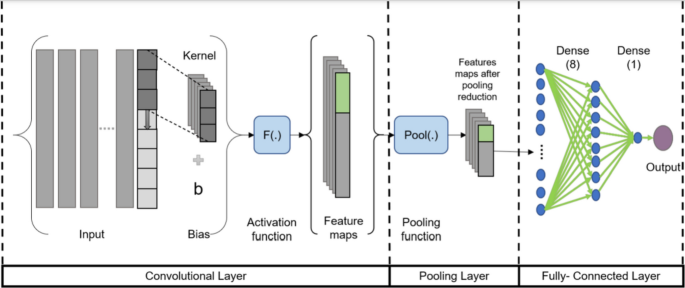
Actually, using a 1D-CNN for time series forecasting involves many steps that are very important to its work. Data from the time series are first preprocessed. For example, due to problems such as normalization and missing values have to be resolved; data sets have also been specially separated into training and testing sets. After that, the data are encoded in a format appropriate for feeding into the 1D-CNN model. Convolutional layers are applied, and filters are moved over the data to create feature maps and extract local patterns. Activation functions and pooling layers, both of which are utilized, are used, respectively, to introduce nonlinearity and reduce dimensionality. After the output of the convolutional layers has been flattened, it is then sent through the fully connected layers, which model high-level relationships and make predictions based on that modeling. The forecasted values are provided by the output layer that comes last [26]. Figure 1 illustrates the main working structure of the 1D-CNN.

Fig. 1

1D-CNN architecture [26]

The CNN layers perform processing on the raw 1D data and “learn to extract” features that are then used by the MLP layers for the classification task that they are responsible for performing. As a direct result, the feature extraction and classification processes are combined into a single procedure, which can then be optimized to achieve the highest possible classification performance. This is the primary benefit of one-dimensional convolutional neural networks 1D-CNNs, which can also result in a low computational burden because the only operation with significant overhead is a sequence of one-dimensional convolutions, which are merely linear weighted sums of two one-dimensional arrays. This results in a simplified computational environment. During the forward-propagation and back propagation operations, it is possible to effectively carry out the linear process in parallel [27].

Following is an expression for 1D forward propagation (1D-FP) that applies to each CNN layer:

$$x_{k}^{l} = b_{k}^{l} + \sum\limits_{i = 1}^{{N_{l - 1} }} {{\text{con}}v1D\left( {w_{ik}^{l - 1} ,s_{i}^{l - 1} } \right)}$$

(1)

$$y_{k}^{l} = f\left( {x_{k}^{l} } \right)\;{\text{and}}\;s_{k}^{l} = y_{k}^{l} \downarrow ss$$

(2)

where the input data can be defined by $x_{k}^{l}$, the bias of the kth neuron at layer $l$ can be defined by $b_{k}^{l}$, $s_{i}^{l - 1}$ represents the ith output of each neuron at $l - 1$ layer, the kernel from the ith neuron at layer $l - 1$ is represented by $w_{ik}^{l - 1}$ to the kth neuron at layer $l$.

The intermediate output, $y_{k}^{l}$, can be expressed by passing the input $x_{k}^{l}$ through the activation function as expressed in Eq. (2). Where $s_{k}^{l}$ represents the output of the kth neuron of the layer $l$, and “$\downarrow {\text{ss}}$” represents the down-sampling operation with a scalar factor, ss.

As an overview, the backpropagation algorithm is as in Eq. (3). Error back propagation begins at the output MLP layer. Assume that the input layer is 1 and the output layer is $l = L$. Then, for an input vector $p$, and its target and output vectors, $t^{p} { }\left[ {y_{1}^{L} , \cdots ,y_{{N_{L} }}^{L} } \right]$, respectively. Let $N_{L}$ be the number of classes in the database. Thus, the mean-squared error (MSE), $E_{p}$, for the input p in the output layer NL can be expressed as follows:

$$E_{p} = {\text{MSE}}\left( {{\varvec{t}}^{p} ,\left[ {y_{1}^{L} , \cdots ,y_{{N_{l} }}^{L} } \right]{\prime} } \right) = \mathop \sum \limits_{i = 1}^{{N_{l} }} \left( {y_{i}^{L} - t_{i}^{p} } \right)^{2}$$

(3)

3.2 Long short-term memory

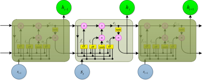
LSTM was developed because standard RNNs struggle to capture long-term relationships in sequential data due to the vanishing gradient problem. The vanishing gradient problem prevents RNNs from learning and modeling sequential data long-term dependencies. Backpropagation forgets data from previous time steps because gradients fall exponentially inside the network. This constraint hinders the RNN’s context learning and memory over time steps. LSTM solves this problem by incorporating a memory cell in the network to preserve and discard data from prior time steps. Memory cells have three gates: input, forget, and output. This gate controls memory cell data interchange, allowing the LSTM to maintain and selectively discard long-term dependence. Memory cell input gates govern data storage. Based on the input and prior hidden state, the network can utilize the sigmoid activation function to choose memory cell data. A sigmoid activation function determines which memory cell data to delete at the forget gate. It calculates the relevance of the prior hidden state and discards forecasting-unneeded data. The output gate controls memory cell data transmission to the hidden state and output using sigmoid activation and hyperbolic tangent functions. This regulates how much data are sent to later periods. LSTM learns and remembers sequential dependencies via these processes [28]. Figure 2 represents the LSTM architecture.

Fig. 2

LSTM architecture [25]

The mathematical representation of the LSTM can illustrated as follows:

$$f_{t} = \sigma \left( {W_{fh} h_{t - 1} + W_{fx} s_{t} + b_{f} } \right)$$

(4)

$$i_{t} = \sigma \left( {W_{ih} h_{t - 1} + W_{ix} s_{t} + b_{i} } \right)$$

(5)

$$\tilde{c}_{t} = \tanh \left( {W_{{\tilde{c}h}} h_{t - 1} + W_{{\tilde{c}x}} s_{t} + b_{{\tilde{c}}} } \right)$$

(6)

$$c_{t} = f_{t} \cdot c_{t - 1} + i_{t} \cdot \tilde{c}_{t}$$

(7)

$$o_{t} = \sigma \left( {W_{oh} h_{t - 1} + W_{ox} s_{t} + b_{o} } \right)$$

(8)

$$h_{t} = o_{t} \cdot \tanh \left( {c_{t} } \right)$$

(9)

where input, recurrent data, and output of each cell at time t can be presented by $x_{t}$, $h_{t}$, and $o_{t}$, respectively. The forget gate is represented by $f_{t}$, $c_{t}$ represents the status of the LSTM’s cell.$W_{f} W_{i}$, $W_{{\tilde{c}}}$, and $W_{o}$ represent the network weights, the operator ‘$\cdot$’ used for the multiplication of two pointwise vectors and $b_{f}$, $b_{i}$, $b_{{\tilde{c}}}$ are the system’s bias.

3.3 Transformer model

The transformer (TF) paradigm revolutionized sequence modeling and is currently employed in numerous domains, including time series analysis [29]. The TF model successfully captures complicated connections and patterns in sequences, making it helpful for sequence data problems. The TF model uses self-attention to focus on numerous sequence places despite vanishing gradients and other limitations. The self-attention mechanism is crucial to the TF design because it helps the model collect long-range relationships and contextual information. The model describes global connections because the full sequence is taken into account. It accomplishes this through relationship-based weighting of extra elements. The attention mechanism allows the TF model to simultaneously consider short-term and long-term dependencies, making its predictions more accurate and therefore reliable. The self-attention and position wise feedforward neural networks used by the TF model implement nonlinear transformations on each sequence position separately. This enables the model to capture complex sequential patterns and interactions, so that it can learn better and predict more accurately. This also assists that the model understands sequences. Because TF parallelizes training and inference, it is particularly suited to large-scale sequence modeling [29].

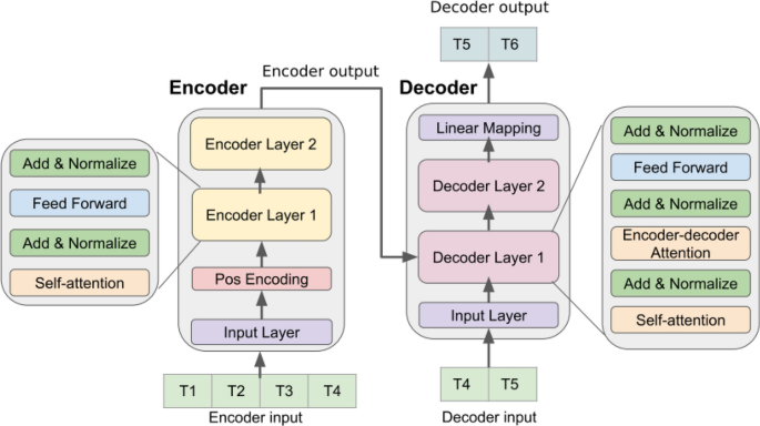
Self-attention and feedforward networks used in the encoding and decoding of TF models record connections, settings, sequences. That is why with the right characteristics, it can excel at many sequence-related tasks like interpreting input sequences and making meaningful output sequences. The TF model’s encoding method is to take a sequence as input and output the encoded representation of that same sequence. This procedure requires several feedforward neural networks and self-attention layers. Each layer begins with the input sequence and uses self-attention to find data interconnections. The self-attention mechanism allows each place in the sequence to pay attention to the others, assigning significance and taking in pertinent background data [29].

Encoding produces encoded representations for decoding. The TF model decodes encoded representations to create a sequence. This level has several self-attention and feedforward neural network layers. In addition to self-attention, encoder-decoder attention is used during decoding. The model can use its encoded representations from the encoding step during decoding. Focusing on the right encoded representations lets the decoder maximize context information from encoding [29]. The TF architecture model is illustrated in Fig. 3.

Fig. 3

Time series transformer forecasting based model architecture [30]

3.4 Hybrid models

Hybrid deep learning models improve time series solar power forecasts. These models use deep learning approaches to increase solar energy system forecast accuracy, interpretability, and robustness.

Hybrid models use deeper learning architectures like LSTM, CNN, and transformer models to capture varied patterns and correlations in solar power time series data. LSTM models long-term dependencies well, CNN extracts spatial information well, and transformers represent global dependencies via attention processes. Hybrid techniques use each architecture’s strengths synergistically to make more accurate predictions. To do this, hybrid techniques combine these models. Traditional forecasting approaches like autoregressive and regression models can also enhance hybrid models. Combining these old methodologies allows interpretability and domain-specific knowledge. This may capture solar power system characteristics that deep learning algorithms struggle with. Hybrid models may enhance forecasts and reveal solar power generating drivers. Combining deep learning’s effective feature extraction and nonlinear modeling with traditional modeling’s interpretability can achieve this. Hybrid models’ improved time series analysis is needed to accurately anticipate solar power and integrate it into the electrical grid. The accurate predictions help in managing resources, stabilizing the grid and planning economically. The hybrid models help in integrating renewable energy sources through addressing issues of solar power forecasting such as complicated connections between solar irradiance, weather and power generation. Hybrid solar power forecasting models make the switch to green power systems easier.

This study aims to improve the accuracy and performance of predictions by investigating various hybrid models that can be used for time series forecasting. The hybrid models that are being investigated include LSTM–TF, TF–LSTM, LSTM–CNN, CNN–LSTM, CNN–TF, TF–CNN, CNN–LSTM–TF, CNN–TF–LSTM, LSTM–CNN–TF, LSTM–TF–CNN, TF–CNN–LSTM, and TF–LSTM–CNN. Every model employs architectures for learning to recognize and leverage different aspects of the data. To illustrate the LSTM TF model amalgamates the strengths of LSTM and TF models. This fusion enables the model to capture both term and global dependencies present, in the data.

On the contrary TF–LSTM places an emphasis, on the TF component to capture connections and dependencies. Simultaneously it harnesses LSTM to capture patterns at a level. The hybrid model, LSTM–CNN combines the strength of LSTM in capturing long term dependencies with CNNs ability to extract spatial features. In this model LSTM is incorporated. However in CNN–LSTM the order is reversed, where CNN takes the lead by extracting features followed by LSTM which models temporal dynamics. This ordering enables outcomes. To consider both global dependencies the CNN–TF model seamlessly integrates CNNs feature extraction capabilities, with TFs self-attention mechanism. The TF–CNN model integrates the TF’s attention mechanism for detecting temporal relationships with the CNN’s capacity for processing spatial data. The CNN–LSTM–TF algorithm combines CNN with LSTM and TF. Using self-attention, this algorithm allows the model to focus on the most important temporal contexts while capturing both local and global dependencies. The CNN–TF–LSTM model puts emphasis on the transformer component and applies LSTM and CNN, respectively, to catch local and global patterns. The LSTM–CNN–TF model can use benefits offered by each of these models by combining them into one model which integrates the capabilities of both LTSM, CNN, TF models in order to consider local, temporal and global dependencies. In this way, this model has an opportunity to benefit from each component. It is a combination of characteristics from the LSTM model, the CNN model and the TF model therefore called TF–CNN–LSTM structure. This hybrid approach captures time-varying phenomena as well as local–global interactions in the data. Hybrid models such as these provide full ways of forecasting time series using their respective forecasting capabilities that leverage on strengths from every part of the model. Consequently, these models have witnessed great improvements in terms of accuracy as well as performance levels.

3.5 Evaluation metrics

Evaluation metrics are used to assess the effectiveness of a predictive model or algorithm. These quantitative measures allow one to evaluate how well a model or algorithm solves a problem. It is possible to develop metrics using both qualitative and quantitative approaches. Additionally, they enable comparison of multiple models or methods by giving objective criteria that can be used to assess the efficacy of a model. Also, evaluation metrics help in making informed judgments concerning the application of a model to a specific task as well as helping determine the overall effectiveness [31]. Consequently, they also aid in assessing whether a given solution’s precision, reliability and generalizability are satisfactory or not.

3.5.1 Mean absolute error (MAE)

The method of evaluation uses the average absolute deviation between observed and predicted values to make a determination. Every variation in the data is given the same importance in this method.

$${\text{MAE}} = \frac{1}{N}\mathop \sum \limits_{i = 1}^{N} \left| {\hat{y}_{i} - y_{i} } \right|$$

(10)

where $\hat{y}_{i}$ is the predicted value of epoch $i$, and $y_{i}$ is the actual value.

3.5.2 Mean square error (MSE)

The difference between the actual and expected values of the model is used in the calculation of this value, and it is then squared. The greater the discrepancies, the more this metric penalizes them.

$${\text{MSE}} = \frac{1}{N}\mathop \sum \limits_{i = 1}^{N} \left( {\hat{y}_{i} - y_{i} } \right)^{2}$$

(11)

3.5.3 Root mean square error (RMSE)

It is used to measure the accuracy of prediction models. In order to determine it, the square root of the mean squared deviations between observed and forecasted values has to be taken into consideration. For this reason, RMSE is widely recognized as a key element of performance evaluation measurement.

$${\text{RMSE}} = \sqrt {\frac{1}{N}\mathop \sum \limits_{i = 1}^{N} \left( {\hat{y}_{i} - y_{i} } \right)^{2} }$$

(12)

3.6 Working structure

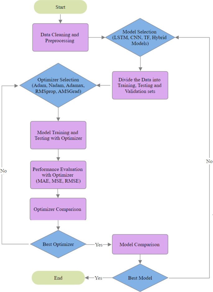
Using relevant time series data initiates the process by capturing changes in solar power generation over time. Preprocessing enhances the quality of data for use in time domain analysis. Model selection introduces a number of architectures, some of which are hybrid combinations designed for time series forecasting and others of which are standalone models like LSTM, CNN, and transformer. After that, the selected models are trained thoroughly with the time series power data, taking into account the temporal dependencies themselves. The use of validation data enhances the training process and guarantees strong model performance. During testing, a different time series dataset is used to assess the models’ capacity to predict solar power generation. In the context of time series forecasting, key performance indicators like MAE, MSE, and RMSE are used for complete evaluation. The optimization process begins with picking an optimizer, which takes time series properties into account. Used optimizers include Adam, Nadam, Adamax, RMSprop, and AMSGrad. The models are then trained and verified using the selected optimizer. After training, the models are tested extensively using the testing time series dataset to determine how well they perform. A decision point is reached after a key model comparison, which identifies the top-performing model for time-domain accurate solar power forecasting. Figure 4 shows the interrelated processes and decision-making procedures that comprise the solar power forecasting system, which is based on time series power data and follows a structured approach.

Fig. 4

Workflow and model selection flowchart

4 Results and discussion

4.1 Data description

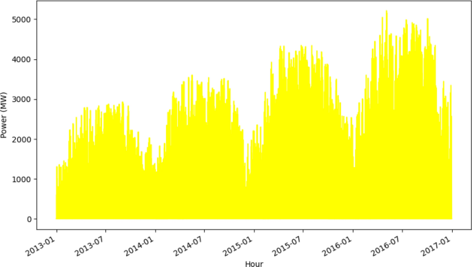
The given dataset has four years of previous solar data. Fundamental understanding of solar power generation in France. This data set includes a detailed analysis based on a comprehensive log of solar power generation, understanding of the solar power scene in the country. Trends, patterns, and thus, one can see variations in solar power generation over the years and seasonal. By analyzing this data, one can identify annual fluctuations, as shown in Fig. 5. They would make clearer patterns of solar power generation. The dataset includes information on solar irradiance levels. Historical solar data are an important factor in time series prediction of solar power generation. It is to formulate models and strategies for exact prediction of future solar events. Patterns and trends revealed in historical data on power production if looked at from this perspective, that information as input.

Fig. 5

Four years solar power records

This study mainly uses time series power data for the purpose of forecasting solar power. But such external factors as changes in weather patterns or improvements in new solar technology are not explicitly considered. To better understand the natural patterns in the timing of solar power generation, time series data were chosen as the primary focus. Furthermore, it is important to note that the forecasting equation takes into account important variables like temperature, solar irradiance, and humidity, among others, because it is based on the mathematical relations that exist between solar power and external factors. The modeling approach incorporates these external factors mathematically, despite the fact that the study does not directly address these external factors. The purpose of the study is to provide insights into the modeling and forecasting performance within the constraints of the time series power data being utilized.

4.2 Experimental setup

An input size consisting of hourly data spanning four years was utilized in the research project. The data were passively split into three groups: training (80%), validation (5%) and testing (15%). The model was tasked with making predictions for the next twenty-four hours. During training, the Mean Squared Error loss function was passively used as a guide to direct the optimization process. A total of 200 epochs were utilized with a learning rate of 0.001, and the training was conducted in a completely unsupervised manner.

A window approach was used, in which the input data were divided into overlapping segments of fixed size, to efficiently manage time series data in the forecasting task. In this instance, the models’ window sizes were set to 5. With this window in place, models can take in more context and relevant information in order to make more precise predictions about the future. To better capture both short-term fluctuations and long-term trends, the models use overlapping windows to take advantage of the sequential nature of the data and learn from previous observations. For time series forecasting, the window approach is indispensable because it helps models grasp the evolution of the data over time, leading to better accuracy in predictions.

This paper explores the 1D CNN, LSTM, and transformer models, as well as all possible hybrid models. These models for time series data have different architectural features and capabilities, the results given in Table 3 are average of 5 runs.

Table 3 Prediction models performance with respect to different optimizers

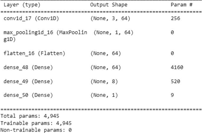
With the 1D CNN as shown in Fig. 6, there is one convolutional layer used in the 1D CNN model with filters of size 3, each one followed by max-pooling, which is excellent at capturing spatial patterns in sequential data. A dense layer containing a single unit for the predicted value serves as the final output layer. With 4,945 total trainable parameters, the 1D CNN model is not overly complex.

Fig. 6

Summary of the 1D CNN model

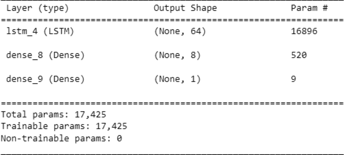
The LSTM model, which is shown in Fig. 7, aims to capture temporal dependencies as accurately as possible. It begins with a single LSTM layer that contains 64 units and then moves on to two dense layers for the purpose of producing an output prediction. The LSTM model is clearly more sophisticated than the 1D CNN in terms of total degree of complexity, as seen by its 17,425 trainable parameters.

Fig. 7

Summary of the LSTM model

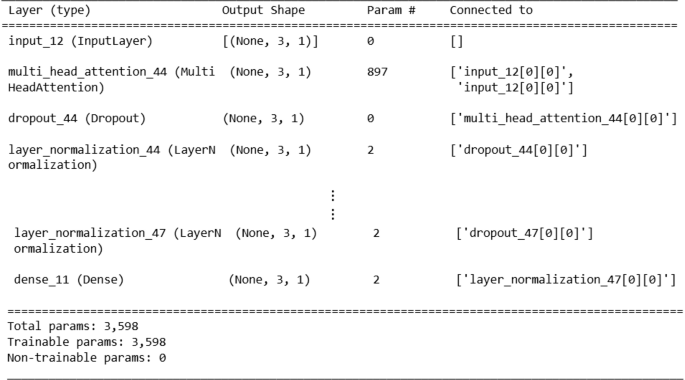
The transformer is depicted in Fig. 8 as an encoder with four multi-head attention layers, each followed by dropout and layer normalization. The attention layers process three-dimensional shape input (None, 3, 1), and a dense output layer with a single unit is utilized to produce predictions in the model. With 3598 trainable parameters, the transformer model is good enough architecture in capturing complicated temporal patterns and enhancing predicting accuracy in time series research.

Fig. 8

Summary of the transformer model

4.3 Numerical results and analysis

Table 3 compares the effectiveness of various prediction models for time series solar power forecasting with different optimizers, all given a score. Models include LSTM, CNN, and TF. In addition to the hybrid models of LSTM–TF, LSTM–CNN, TF–LSTM, CNN–LSTM, CNN–TF and so on. These models are evaluated on the basis of MAE, MSE and RMSE. And also, different optimizers like Adam, Nadam, Adamax and RMSprop were employed to test the prediction model for time series solar power forecasting.

According to the table, it is evident that the CNN–LSTM–TF model when using the Nadam optimizer is by far the best model. It achieves lowest error values of 0.551% MD AE (mean average error) and clearly demonstrates its superiority as a forecasting method for solar power time series data. It is important to note that using different optimizers can affect models in other ways also. In this instance, Nadam proved to be best for the CNN–LSTM–TF model used for solar power forecasting.

Adam may not be the best optimizer for the CNN–LSTM–TF model, but it’s results are still respectable enough to be mentioned. Although Adam did well for the CNN–LSTM–TF model, the Nadam optimizer did even better in terms of prediction accuracy. The differences between Adam and Nadam can be traced back to the optimization algorithms’ divergent abilities to converge on optimal solutions appropriate to the specified model architecture and dataset.

The table demonstrates that the Adam optimizer yielded an MAE value of 16.17% with a TF–LSTM model. This suggests that the differences between model predictions and observed values were larger on average than with any other model or optimizer in this study. This rather high MAE for the TF–LSTM model with Adam hints that the model cannot well rely on accurately capturing patterns and trends in solar power time series data.

Compared with other models for time series solar power forecasting (namely LSTM, CNN and TF), using different optimizers, the determination was that it was always LSTM. A comparison of the LSTM model’s MAE, MSE and RMSE to those for the CNN and the TF led to one clear conclusion-the LSTM beat both. It explains why LSTM is better at extracting the kinds of temporal relationships and even patterns that are inherent in solar power data, making forecasting models more effective. Unlike CNN and TF models, all optimizers showed rising error rates and lower performance levels. In terms of generating trustworthy predictions about future solar power generation, according to these studies, the LSTM model is by far the best alternative when compared with other prediction models such as the CNN and TF models. This is the case in a comparison of the LSTM model with compared to a CNN model and a TF model.

By applicable use of a trick version of this optimizer, we led down the MAE for solar power forecasting across time series to 0.5886%. And this illustrates that the model can accurately predict future solar power generation. This helps explain why the hybrid model performs better than others. Its creation involved combining TF, LSTM and CNN components. One of the more useful qualities of the model’s LSTM component is its ability to simulate temporal dynamics, while its capability of capturing short-term dependencies at one time lies in its transformer component. The second would be that by using it, our model has much larger global volume and range than RNN/LSTM models; it can also catch long-term patterns which are not from a local to spatial level, the CNN module enables pattern tracking in time series data. But as it combines the two methods, the TF–LSTM–CNN model will be able to effectively identify seasonality and time series feature dependence in solar power data. A better ability to forecast means training and optimizing the model are improved. By using RMSprop as an optimizer, this is accomplished. Thus, the TF–LSTM–CNN model optimized using RMSprop has emerged as a highly mature and stable method for forecasting solar power time series. In addition, the MAE value for using AMSGrad optimizer and training on the LSTM–TF–CNN model was 0.6087%. This shows the model’s ability to predetermine precisely how much electricity will be generated by solar power 20 h hence.

The results should show the importance of how the 15 models match up with different optimizers. It can be seen that four times they were the best optimizers for the model, so the operation of optimizing the model parameters was undoubtedly quite successful. Also known as Adam, the algorithm is widely praised for its learning rates which respect a user-specified minimum but vary with execution time; it also generates momentum to make convergence quicker and reduce overfitting. To boost the convergence rate even more, the Nesterov momentum is added to Nadam, a combination of Nesterov accelerated gradient and Adam. Both optimizers have demonstrated that they can produce decent results from more than one model.

RMSprop, on the other hand, was picked as the top optimizer three times. Because it changes the learning rate based on the root mean square of recent climbs, RMSprop is well-suited for managing sparse data and noisy gradients. Its constant performance demonstrates that it may be used to refine model parameters in jobs involving solar power forecasts over time.

AMSGrad and Adamax worked out best as optimizers, for two separate models. An Adam-type algorithm, namely, the infinity norm is used to obtain an adaptive learning rate. A smooth problem is a modification of the Adam procedure where there is always some bound on the accumulation of terms. The changing of this is to enhance the convergence properties. First, these optimizers not only outperformed all other models but indeed beat the target forecast by 3–4% points. Secondly and most importantly, their success in overcoming such difficulties as time series solar power forecasts attests how well they have solved these special problems.

4.4 A comparison between the best (CNN–LSTM–TF) and the worst model (TF–LSTM)

When comparing the 15 models, significant differences in performance were found, with the CNN–LSTM–TF model coming out on top and the TF–LSTM model coming in last. With an astoundingly small MAE of 0.551%, the CNN–LSTM–TF model showed off impressive accuracy in the case of Nadam. This means that the model was, on average, quite accurate in its predictions. The model also displayed an extremely small MSE of 0.01%, which is strong evidence that it successfully captured the underlying patterns in the data.

Meanwhile, the TF–LSTM model based on Adam had a MAE of 16.17% and an MSE of 3.642%, showing that it could not predict well enough to earn profits than feeding living fish to the fish market in exchange for cash. A large prediction error the root-mean-squared (RMS) error was 19.085%. These results demonstrate that the model was unable to get at the nuances of how and in what ways data were related.

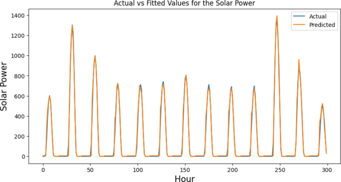
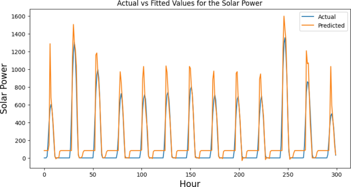
Figure 9, which illustrates the actual versus fitted values of the CNN–LSTM–TF model, shows a comparison between the actual values of the solar power data and the values that the CNN–LSTM–TF model predicted. Figure 10, on the other hand, shows the TF–LSTM model’s actual values versus its fitted values. It is similar to Table 3, and demonstrates how the actual outcomes of solar power data compare with predicted values. These inconsonant results serve to bring to light the importance of model selection and appraisal in time series forecasting. The Solar Power Forecasting Game It seems that the TF–LSTM model has limitations in accurately representing the solar power data. In contrast, the CNN–LSTM–TF model demonstrates a good fit to the data.

Fig. 9

Actual versus fitted values of the CNN–LSTM–TF model

Fig. 10

Actual versus fitted of the TF–LSTM model

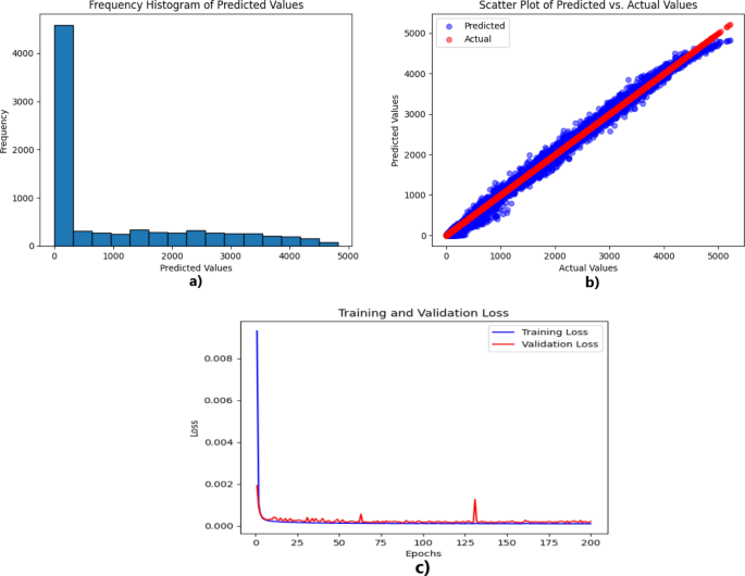
Figure 11 includes three subplots: (a) the CNN–LSTM–TF frequency histogram of predicted values; (b) the scatter plot of predicted versus actual values; and (c) the training and validation loss plot. This figure provides a comprehensive analysis of the CNN–LSTM–TF model, which is recognized as the model with the highest level of performance accuracy.

Fig. 11

CNN–LSTM–TF model performance, a frequency histogram of predicted values. b The scatter plot of predicted versus actual values. c The training and validation loss plot

In Fig. 11a, the frequency histogram of predicted values shows how the model’s predictions are distributed. A well-fitted model should have a histogram that closely matches the distribution of actual values. In this case, the histogram shows a strong match between predicted and actual values. This demonstrates that the CNN–LSTM–TF model properly captures the fundamental patterns and trends in solar power data. A scatter plot in Fig. 11b contrasts expected and actual values. If the model is well-fitted, the data points will be firmly grouped along the diagonal line. This shows that the predicted and actual values are closely related. In this plot, the data points are closely spaced along the diagonal, which suggests that the model’s predictions are accurate and consistent. Figure 11c is the training and validation loss plot. This graph shows how well the model performed during the training phase. The loss values show the difference between the predicted and actual values. A well-fitted model should show a downward trend in both the training and validation losses. In this case, the CNN–LSTM–TF model has consistently low loss values, which shows that it can effectively reduce the difference between the predicted and actual values.

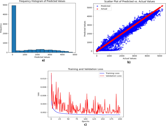
Figure 12 has three subplots: (a) TF–LSTM frequency histogram of predicted values, (b) scatter plot of predicted vs. actual values, and (c) training and validation loss plot. Even though the results show that the TF–LSTM model is the worst, the numbers show that it differs significantly from the actual values. The frequency histogram appears a bit like how the actual values are spread out, but the scatter plot shows that the data points are more spread out away from the diagonal line. This shows that the model’s predictions are not very accurate or precise. Also, the training and validation loss plots show higher values, suggesting that the predicted and actual values differ.

Fig. 12

TF–LSTM model performance, a frequency histogram of predicted values. b The scatter plot of predicted versus actual values. c The training and validation loss plot

5 Conclusion

Predicting solar output is crucial for the future of renewable energy and ecological progress. Solar power has the potential to significantly contribute to the world’s energy mix and lessen reliance on fossil fuels because it is both valuable and plentiful. However, solar energy’s intermittent and unpredictable nature prevents its effective incorporation into the power grid. Integration, planning, and operation of solar power systems are greatly aided by accurate solar power forecasting. It helps keep the grid stable, promotes effective energy management, streamlines market entry, and provides input for policymaking. Forecasting aids the worldwide movement toward a sustainable, low-carbon future by facilitating more efficient use of solar resources.

Many energy management and decision-making facets benefit greatly from accurate solar power forecasting. The effectiveness of hybrid models in capturing the complex patterns inherent in the data is highlighted by comparing deep learning models for time series forecasting of solar energy systems. The CNN–LSTM–TF model using the Nadam optimizer shows the greatest improvement over the other models, with an MAE of 0.551%. This unique model brings together the advantages of using 1D-CNN to extract spatial features, LSTM to understand temporal patterns, and the transformer to analyze global connections. The data also show how the performance of the model varies depending on which optimizer is used, with Nadam and Adam consistently producing the best results. However, when it comes to forecasting solar power, the TF–LSTM model implemented with the Adam optimizer faces more challenges in providing accurate predictions. By consistently outperforming CNN and TF models, the LSTM model demonstrates its superior ability to capture temporal relationships. The performance of the TF–LSTM–CNN model is enhanced by utilizing the RMSprop optimizer, leading to a decrease in the mean absolute error (MAE) to an impressively low value of 0.5886%. Similarly, when employing the AMSGrad optimizer, the LSTM–TF–CNN model also achieves an exceptionally low MAE of 0.6087%. These findings illuminate the significance of selecting an appropriate model and optimizer in the realm of solar power forecasting. Furthermore, they offer valuable insights for optimizing and strategizing renewable energy systems. Furthermore, the findings provide useful suggestions for researchers, industry experts, and policymakers to apply these models to improve the efficiency and integration of solar energy systems.

The use of hybrid deep learning models in this study improves the accuracy of solar power forecasts. However, it is critical to acknowledge and understand the limits of our method. Because of the time series power dataset used in the study, these models may not be relevant in other scenarios. To solve this constraint, future research should focus more on studying varied datasets to evaluate model dependability across multiple data circumstances. Although the inquiry is helpful, it does not do an analysis of all of the hyperparameters, which may cause it to ignore the configurations that give the best results. A detailed evaluation of hyperparameters is essential to acquire a full knowledge of the model’s performance in future research. Such factors aid in improving and widening our methods for future research aims. Moreover, it is possible that future research in the field of solar power forecasting will concentrate on integrating advanced machine learning techniques, investigating synergies between various models, and investigating temporal dynamics in order to produce more accurate results. Furthermore, the investigation of the impact of emerging technologies such as advanced weather modeling on solar forecasting holds the promise of further refinement and innovation in the methodologies used to predict solar power.

References

J Zheng 2020 Time series prediction for output of multi-region solar power plants Appl Energy 257 114001
H Sharadga S Hajimirza RS Balog 2020 Time series forecasting of solar power generation for large-scale photovoltaic plants Renew Energy 150 797 807
C Wan J Zhao Y Song Z Xu J Lin Z Hu 2016 Photovoltaic and solar power forecasting for smart grid energy management CSEE J Power Energy Syst 1 4 38 46
H Ye B Yang Y Han N Chen 2022 State-of-the-art solar energy forecasting approaches: critical potentials and challenges Front Energy Res 10 1 5
P Kumari D Toshniwal 2021 Deep learning models for solar irradiance forecasting: a comprehensive review J Clean Prod 318 128566
J Sharma 2022 A novel long term solar photovoltaic power forecasting approach using LSTM with Nadam optimizer: a case study of India Energy Sci Eng 10 8 2909 2929
Mulyadi A, Djamal EC (2019) Sunshine duration prediction using 1D convolutional neural networks. In: Proceedings of 2019 6th international conference on instrumentation, control, and automation (ICA), pp 77–81
EM Al-Ali 2023 Solar energy production forecasting based on a hybrid CNN–LSTM–transformer model Mathematics 11 3 1 19
NE Benti MD Chaka AG Semie 2023 Forecasting renewable energy generation with machine learning and deep learning: current advances and future prospects Sustainability 15 9 7087
RA Rajagukguk RAA Ramadhan HJ Lee 2020 A review on deep learning models for forecasting time series data of solar irradiance and photovoltaic power Energies 13 24 6623
M Husein IY Chung 2022 Day-ahead solar irradiance forecasting for microgrids using a long short-term memory recurrent neural network: a deep learning approach Energies 12 1856
M Elsaraiti A Merabet 2022 Solar power forecasting using deep learning techniques IEEE Access 10 31692 31698
EG Kim MS Akhtar OB Yang 2023 Designing solar power generation output forecasting methods using time series algorithms Electr Power Syst Res 216 109073
Sana Amreen T, Panigrahi R, Patne NR (2023) Solar power forecasting using hybrid model. In: 2023 5th International conference on energy, power and environment: towards flexible green energy technologies (ICEPE), pp. 1–6
K Wang 2019 Multiple convolutional neural networks for multivariate time series prediction Neurocomputing 360 107 119
Z Zhao 2021 Short-term load forecasting based on the transformer model Information 12 12 1 22
M Aslam, KH Seung, S Jae Lee, JM Lee, S Hong, EH Lee (2019) Long-term solar radiation forecasting using a deep learning approach-GRUs. In: 2019 IEEE 8th international conference on advanced power system automation and protection (APAP), pp. 917–920
Zhao, Y., Wang, G., Tang, C., Luo, C., Zeng, W., & Zha, Z. J. (2021). A battle of network structures: An empirical study of cnn, transformer, and mlp. arXiv preprint. https://doi.org/10.48550/arXiv.2108.13002
X Song 2020 Time-series well performance prediction based on long short-term memory (LSTM) neural network model J Pet Sci Eng 186 106682
ES Al-Abri 2018 Modelling atmospheric ozone concentration using machine learning algorithms PLoS ONE 13 3 e0194889
V Suresh P Janik J Rezmer Z Leonowicz 2020 Forecasting solar PV output using convolutional neural networks with a sliding window algorithm Energies 13 3 723
H Chen X Chang 2021 Photovoltaic power prediction of LSTM model based on Pearson feature selection Energy Rep 7 1047 1054
NW Kim HY Lee JG Lee BT Lee 2021 Transformer based prediction method for solar power generation data Int Conf ICT Converg 2021 7 9
G Li S Xie B Wang J Xin Y Li S Du 2020 Photovoltaic power forecasting with a hybrid deep learning approach IEEE Access 8 175871 175880
X Wang X Li K Yang Z Huang 2019 A blind spectrum sensing method based on deep learning Nature 29 7553 1 73
N Vakitbilir A Hilal C Direkoğlu 2022 Hybrid deep learning models for multivariate forecasting of global horizontal irradiation Neural Comput Appl 34 10 8005 8026
S Kiranyaz O Avci O Abdeljaber T Ince M Gabbouj DJ Inman 2021 1D convolutional neural networks and applications: a survey Mech Syst Signal Process 151 107398
R. C. Staudemeyer and E. Rothstein Morris, ‘‘Understanding LSTM - a tutorial into long short-term memory recurrent neural networks,’’ 2019, arXiv:1909.09586. https://doi.org/10.48550/arXiv.1909.09586
A Veltman DWJ Pulle RW Doncker De 2017 Attention is all you need Power Syst 30 47 82
Wu, N., Green, B., Ben, X., & O'Banion, S. (2020). Deep transformer models for time series forecasting: The influenza prevalence case. arXiv preprint. https://doi.org/10.48550/arXiv.2001.08317
H Dalianis 2018 Evaluation metrics and evaluation Clin Text Min 1967 45 53
Huang W (2019) Historical data in simulation (Data in France). Figshare, London
Funding
Open access funding provided by the Scientific and Technological Research Council of Türkiye (TÜBİTAK). This study was performed with the support of Cyprus International University.
Author information
Authors and Affiliations
Contributions
Conceptualization, DS, CD, MK and MF; methodology, DS and CD; software, DS and CD; validation, DS and CD; formal analysis, DS, CD, MK and MF; investigation, DS and MK; resources, DS, CD, MK and MF; data curation, DS and MK; writing—original draft preparation, DS; writing—review and editing, DS; visualization, DS, CD, MK and MF; supervision, CD, MK and MF; project administration, DS.
Corresponding author
Ethics declarations
Conflict of interest
The authors declare no conflicts of interest.
Ethical approval
Not Applicable.
Informed consent
Additional information
Publisher's Note
Springer Nature remains neutral with regard to jurisdictional claims in published maps and institutional affiliations.
Rights and permissions
Open Access This article is licensed under a Creative Commons Attribution 4.0 International License, which permits use, sharing, adaptation, distribution and reproduction in any medium or format, as long as you give appropriate credit to the original author(s) and the source, provide a link to the Creative Commons licence, and indicate if changes were made. The images or other third party material in this article are included in the article's Creative Commons licence, unless indicated otherwise in a credit line to the material. If material is not included in the article's Creative Commons licence and your intended use is not permitted by statutory regulation or exceeds the permitted use, you will need to obtain permission directly from the copyright holder. To view a copy of this licence, visit http://creativecommons.org/licenses/by/4.0/.
About this article
Cite this article
Salman, D., Direkoglu, C., Kusaf, M. et al. Hybrid deep learning models for time series forecasting of solar power. Neural Comput & Applic 36, 9095–9112 (2024). https://doi.org/10.1007/s00521-024-09558-5
Received:
Accepted:
Published:
Issue Date:
DOI: https://doi.org/10.1007/s00521-024-09558-5