An inexact regularized proximal Newton method for nonconvex and nonsmooth optimization

Abstract

This paper focuses on the minimization of a sum of a twice continuously differentiable function f and a nonsmooth convex function. An inexact regularized proximal Newton method is proposed by an approximation to the Hessian of f involving the $\varrho$th power of the KKT residual. For $\varrho =0$, we justify the global convergence of the iterate sequence for the KL objective function and its R-linear convergence rate for the KL objective function of exponent 1/2. For $\varrho \in (0,1)$, by assuming that cluster points satisfy a locally Hölderian error bound of order q on a second-order stationary point set and a local error bound of order $q>1\!+\!\varrho$ on the common stationary point set, respectively, we establish the global convergence of the iterate sequence and its superlinear convergence rate with order depending on q and $\varrho$. A dual semismooth Newton augmented Lagrangian method is also developed for seeking an inexact minimizer of subproblems. Numerical comparisons with two state-of-the-art methods on $\ell _1$-regularized Student’s t-regressions, group penalized Student’s t-regressions, and nonconvex image restoration confirm the efficiency of the proposed method.

1 Introduction

Given a data matrix $A\in {\mathbb {R}}^{m\times n}$ and a vector $b\in {\mathbb {R}}^{m}$, we are interested in the following nonconvex and nonsmooth composite optimization problem

$$\begin{aligned} \min _{x\in {\mathbb {R}}^n}F(x):=f(x)+g(x)\quad \textrm{with}\quad f(x):=\psi (Ax-b), \end{aligned}$$

(1)

where $\psi \!:{\mathbb {R}}^m\rightarrow \overline{{\mathbb {R}}}$ and $g\!:{\mathbb {R}}^n\rightarrow \overline{{\mathbb {R}}}$ with $\overline{{\mathbb {R}}}\!:=(-\infty ,\infty ]$ are proper lower semicontinuous (lsc) functions and satisfy the following basic assumption:

Assumption 1

• (i) $\psi$ is twice continuously differentiable on an open set containing $A({\mathcal {O}})-b$, where ${\mathcal {O}}\subset {\mathbb {R}}^n$ is an open set covering the domain ${\textrm{dom}}\,g$ of g;

• (ii) g is convex and continuous relative to ${\textrm{dom}}\,g$;

• (iii) F is coercive, i.e., for every $\{x^k\}\subset {\textrm{dom}}\,g$ with $\Vert x^k\Vert \rightarrow \infty$, $\lim _{k\rightarrow \infty }F(x^k)=\infty$.

Assumption 1 (ii) means that model (1) allows g to be an indicator function of a closed convex set in ${\mathbb {R}}^n$, and it also covers the case that g is a weakly convex function. Indeed, by recalling that g is $\alpha$-weakly convex if $g(\cdot )\!+\!(\alpha /2)\Vert \cdot \Vert ^2$ is convex for some $\alpha \ge 0$, F can be rewritten as $F={\overline{f}}\!+\!{\overline{g}}$ with ${\overline{f}}(\cdot )\!=f(\cdot )\!-\!(\alpha /2)\Vert \cdot \Vert ^2$ and ${\overline{g}}(\cdot )\!=g(\cdot )\!+\!(\alpha /2)\Vert \cdot \Vert ^2$. Note that ${\overline{f}}$ can be reformulated as ${\overline{\psi }}({\overline{A}}\cdot -{\overline{b}})$ for suitable ${\overline{A}}$ and ${\overline{b}}$ with ${\overline{\psi }}(\cdot )=\psi (\cdot )-(\alpha /2)\Vert \cdot \Vert ^2$. Hence, ${\overline{f}}$ and ${\overline{g}}$ conform to Assumption 1. As ${\textrm{dom}}\,F={\textrm{dom}}\,g$ is closed, Assumption 1 (iii) ensures that problem (1) has an optimal solution and then a stationary point.

Model (1) has a host of applications in statistics, signal and image processing, machine learning, financial engineering, and so on. For example, the popular lasso [1] and sparse inverse covariance estimation [2] in statistics are the special instances of (1) with a convex $\psi$. In some inverse problems, non-Gaussianity of noise or nonlinear relation between measurements and unknowns often leads to (1) with a nonconvex $\psi$ (see [3]). In addition, the higher moment portfolio selection problem (see [4, 5]) also takes the form of (1) with a nonconvex $\psi$.

1.1 Related works

For problem (1), many types of methods have been developed. Fukushima and Mine [6] introduced originally the proximal gradient (PG) method; Tseng and Yun [7] proposed a block coordinate decent method and obtained the subsequence convergence of the iterate sequence and its R-linear convergence rate under the Luo–Tseng error bound; Milzarek [8] developed a class of methods by virtue of a combination of semismooth Newton steps, a filter globalization, and thresholding steps for (1) with $g(x)=\mu \Vert x\Vert _1$, and achieved subsequence convergence and local q-superlinear convergence properties for $q\in (1,2]$; Bonettini et al. [9] extended their variable metric inexact line-search (VMILA) method [10] by incorporating a forward–backward step, and verified the global convergence of the iterate sequence and the linear convergence rate of the objective value sequence under the uniformly bounded positive definiteness of the scaled matrix and the KL property of exponent $\theta \in (0,1/2]$ of the forward–backward envelope (FBE) of F; and by using the FBE of F, initially introduced in [11], Stella et al. studied a combination of PG step and quasi-Newton step of FBE of F with a line search at the iterate, verified the global convergence for a KL function F and the superlinear convergence rate under the nonsingularity of the Hessian of the FBE in [12], and obtained the same properties as in [12] for (1) but with a nonconvex g by using an Armijo line search at the PG output of iterate in [13].

Next we mainly review inexact proximal Newton methods that are closely related to this work. This class of methods, also called an inexact successive quadratic approximation method, is finding in each iterate an approximate minimizer $y^k$ satisying a certain inexactness criterion for a subproblem of the following form

$$\begin{aligned} \mathop {\min }_{x\in {\mathbb {R}}^n} \Theta _k(x)\!:=\!f(x^k)+\langle \nabla \!f(x^k),x-\!x^k\rangle +\frac{1}{2}(x\!-x^k)^{\top }G_k(x\!-\!x^k)+g(x), \end{aligned}$$

(2)

where $x^k$ is the current iterate, and $G_k$ is a symmetric positive definite matrix that represents a suitable approximation of the Hessian $\nabla ^2\!f(x^k)$. The proximal Newton method can be viewed as a special variable metric one, and it will reduce to the PG method if $G_k\!=\!\gamma _k I$ with $\gamma _k>0$ related to the Lipschitz constant of $\nabla \!f$. Note that subproblem (2) is seeking a root of $0\in \nabla \!f(x^k)+G_k(x-x^k)+\partial g(x)$, the partially linearized version at $x^k$ of the stationary point equation $0\in \partial F(x)$, where $\partial F(x)$ denotes the basic (limiting or Mordukhovich) subdifferential of F at x. The proximal Newton method belongs to the quite general iterative framework proposed by Fischer [14] if the inexactness criterion there is used, but it is not implementable due to the involved unknown stationary point set. As pointed out in [15], the proximal Newton method depends more or less on three key ingredients: the approximation matrix $G_k$, the inner solver to subproblem (2), and the inexactness criterion on $y^k$ (i.e., the stopping criterion of the inner solver to control the inexactness of $y^k$). Since (2) takes into account the second-order information of f, the proximal Newton method has a remarkable superiority to the PG method, i.e., a faster convergence rate.

Early proximal Newton methods were tailored for special instances of convex $\psi$ and g in problem (1) such as GLMNET [16], newGLMNET [17], QUIC [18] and the Newton–Lasso method [19]. Lee et al. presented a generic version of the exact proximal Newton method in [20], achieved a global convergence result by requiring the uniform positive definiteness of $G_k$, and established a local linear or superlinear convergence rate depending on the forcing term on a stopping criterion for an inexact proximal Newton method with unit step-size. Li et al. [21] extended the exact proximal Newton method proposed in [22] for self-concordant functions f to the proximal Newton method with inexact steps, and achieved the local linear, superlinear or quadratic convergence rate resting with the parameter in the inexact criterion under the positive definiteness assumption of $\nabla ^2\!f$ on ${\textrm{dom}}\,f$. Yue et al. [15] proposed an inexact proximal Newton method with a regularized Hessian by an inexactness condition depending on the KKT residual of the original problem, and established the superlinear and quadratic convergence rates under the Luo–Tseng error bound. As far as we know, their work is the first to achieve the superlinear convergence without the strong convexity of F for an implementable proximal Newton method, though Fisher [14] ever got the superlinear convergence rate for the proposed iterative framework, covering the proximal Newton method with an impractical inexactness criterion, under the calmness of the mapping $(\partial F)^{-1}$. Mordukhovich et al. [23] also studied a similar inexact regularized proximal Newton method, and achieved the R-superlinear convergence rate under the metric q-subregularity of $\partial F$ for $q\in (\frac{1}{2},1)$, and the quadratic convergence rate under the metric subregularity of $\partial F$ that is equivalent to the calmness of $(\partial F)^{-1}$. Their metric q-subregularity condition is weaker than the Luo–Tseng error bound.

For problem (1) with $g(x)=\mu \Vert x\Vert _1$, Byrd et al. [24] studied an inexact proximal Newton method with an approximate solution criterion determined by the KKT residual of (1). They showed that the KKT residual sequence converges to zero under the uniformly bounded positive definiteness of $G_k$ and obtained local superlinear and quadratic convergence rates under the positive definiteness and the Lipschitz continuity of $\nabla ^2\!f$ at stationary points. For (1) with an optimal-set-strongly-convex F, Lee and Wright [25] investigated an inexact proximal Newton method with an approximate solution criterion relying on the difference between the objective function value of (2) at the iterate and its optimal value and established a global linear convergence rate of the objective value sequence under the uniformly bounded positive definiteness of $G_k$. Recently, Kanzow and Lechner [26] proposed a globalized inexact proximal Newton-type (GIPN) method by switching from a Newton step to a PG step when the proximal Newton direction does not satisfy a sufficient decrease condition, and established the global convergence and superlinear convergence rate under the uniformly bounded positive definiteness of $G_k$ and the local strong convexity of F.

From the above discussions, we see that for the nonconvex problem (1), the existing global convergence results of the proximal Newton methods require the uniform positive definiteness of $G_k$, while the local superlinear (or quadratic) convergence results assume that F is locally strongly convex in a neighborhood of cluster points of the iterate sequence. The local strong convexity of F in a neighborhood of a stationary point implies the isolatedness of this stationary point, and then the Luo–Tseng error bound and subsequently the metric subregularity of the mapping $\partial F$. Inspired by the works [15, 23], it is natural to ask whether an inexact proximal Newton method can be designed for problem (1) to possess a superlinear convergence rate without the local strong convexity of F. In addition, we observe that when the power $\varrho = 0$ in the regularized Hessian (3) below, the global convergence of the iterate sequence in [15] requires the Luo–Tseng’s error bound as does for its linear convergence rate, and in addition their linear convergence rate result depends upon that the parameter of the method is upper bounded by the unknown constant of the error bound. Then, it is natural to ask whether it is possible to achieve the global convergence and linear convergence rate of the iterate sequence for (1) under a weaker condition. This work aims to resolve these two questions for the nonconvex and nonsmooth problem (1).

1.2 Our contributions

Motivated by the structure of f and the work [27] for a smooth unconstrained problem, we adopt the following regularized version of the Hessian $\nabla ^2f(x^k)$:

$$\begin{aligned} G_k=\!\nabla ^2\!f(x^k)+a_1[-\lambda _{\textrm{min}}(\nabla ^2\psi (Ax^k\!-\!b))]_{+}A^{\top }\!A+a_2[r(x^k)]^{\varrho }I \end{aligned}$$

(3)

to construct a strongly convex approximation of F at iterate $x^k$, and propose an inexact regularized proximal Newton method (IRPNM) for (1), where $a_{+}\!:=\max (0,a)$ for $a\in {\mathbb {R}}$, $\lambda _{\textrm{min}}(H)$ denotes the smallest eigenvalue of H, $r(x^k)$ is the KKT residual of (1) at $x^k$ (see (4) for its definition), and $a_1\!\ge 1,a_2\!>0$ and $\varrho \in [0,1)$ are the constants. Different from the regularized Hessian in [27], we here use $a_1[-\lambda _{\textrm{min}}(\nabla ^2\psi (Ax^k\!-\!b))]_{+}A^{\top }\!A$ to replace $a_1[-\lambda _{\textrm{min}}(\nabla ^2\!f(x^k))]_{+}I$ in order to avoid the computation of the smallest eigenvalue when $\psi$ is separable, i.e., $\psi (y)\!:=\sum _{i=1}^m\psi _i(y_i)$ with each $\psi _i:{\mathbb {R}}\rightarrow \overline{{\mathbb {R}}}$ being twice continuously differentiable on a suitable set. The matrix $G_k$ in (3) is uniformly positive definite when $\varrho = 0$ but not when $\varrho \in (0,1)$ because $r(x^k)\rightarrow 0$ as $k\rightarrow \infty$ as will be shown later. Our inexactness criterion on $y^k$ depends on the nonincreasing of the objective value of (2), along with the KKT residual $r(x^k)$ when $\varrho \in (0,1)$ and the approximate optimality of $y^k$ when $\varrho =0$; see criteria (13a) and (13b) below. In addition, the Armijo line search is imposed on the direction $d^k\!:=y^k-x^k$ to achieve a sufficient decrease of F. Our contributions are summarized as follows.

For $\varrho =0$, we achieve a global convergence of the iterate sequence for the KL function F and its R-linear convergence rate for the KL function F of exponent 1/2, which is weaker than the Luo–Tseng error bound. In this case, our regularized proximal Newton method is similar to the VMILA in [3, 9] except that a different inexactness criterion and a scaled matrix involving the Hessian of f are used. Compared with the convergence results in [9], which removes the restriction condition (see [3, Eq. (23)]) on the iterate sequence in the convergence analysis of [3], our R-linear convergence rate is obtained for the iterate sequence instead of the objective value sequence, and the required KL property of exponent 1/2 is for F itself rather than its FBE. Though by [28, Remark 5.1(ii)] the KL property of F with exponent 1/2 at ${\overline{x}}\in {\textrm{dom}}\,\partial F$ implies that of its FBE $F_{\gamma }$ at ${\overline{x}}$, this requires imposing a restriction on the parameter $\gamma$, i.e., $\gamma$ is smaller than the inverse of the Lipschitz modulus of $\nabla \!f$ at ${\overline{x}}$.

For $\varrho \in (0,1)$, we establish the global convergence of the iterate sequence and its superlinear convergence rate with order $q(1\!+\!\varrho )$, under an assumption that cluster points satisfy a locally Hölderian error bound of order $q\in (\max \{\varrho ,(1\!+\!\varrho )^{-1}\},1]$ on a second-order stationary point set. This result not only extends the conclusion of [23, Theorem 5.1] to problem (1), but also discards the local strong convexity required in the convergence analysis of the (regularized) proximal Newton methods for this class of nonconvex and nonsmooth problems [24, 26]. When cluster points satisfy a local error bound of order $q>1\!+\!\varrho$ on the common stationary point set, we also achieve the global convergence of the iterate sequence and its superlinear convergence rate of order ${(q-\varrho )^2}/{q}$ for $q>[\varrho +\!1/2+\!\sqrt{\varrho +\!1/4}]$, which bridges the gap that the second-order stationary point set may be empty. Compared with the superlinear convergence results in [13] for the hybrid method of the PG steps and quasi-Newton steps of FBE of F, ours do not require twice epi-differentiability of g and the strong local optimality of the limit (which is actually an isolated local minimizer), though there is no direct implication between our local error bound condition and their Dennis–Moré condition.

In addition, inspired by the structure of $G_k$, we also develop a dual semismooth Newton augmented Lagrangian method (SNALM) to compute the approximate minimizer $y^k$ of (2) satisying the inexactness criterion (13a), and compare the performance of our IRPNM armed with SNALM with that of GIPN [26] and ZeroFPR [13] on $\ell _1$-regularized Student’s t-regressions, group penalized Student’s t-regressions and nonconvex image restoration. Numerical comparisons indicate that IRPNM is superior to GIPN in the objective value and the running time, and it is comparable with ZeroFPR in terms of the objective value, but requires much less running time than ZeroFPR if the obtained stationary point is a second-order one (such as for $\ell _1$-regularized and group penalized Student’s t-regressions), otherwise requires more running time than the latter (such as for nonconvex image restoration). Such a numerical performance is entirely consistent with the theoretical results.

1.3 Notations

Throughout this paper, ${\mathbb {S}}^n$ represents the set of all $n\times n$ real symmetric matrices, ${\mathbb {S}}_{+}^n$ denotes the cone consisting of all positive semidefinite matrices in ${\mathbb {S}}^n$, and I denotes an identity matrix whose dimension is known from the context. For a real symmetric matrix H, $\Vert H\Vert$ denotes the spectral norm of H, and $H\succeq 0$ means that $H\in {\mathbb {S}}_{+}^n$. For a closed set $C\subset {\mathbb {R}}^n$, $\Pi _{C}$ denotes the projection operator onto the set C, ${\textrm{dist}}(x,C)$ means the Euclidean distance of a vector $x\in {\mathbb {R}}^n$ to the set C, and $\delta _{C}$ denotes the indicator function of C. For a vector $x\in {\mathbb {R}}^n$, ${\mathbb {B}}(x,\delta )$ denotes the closed ball centered at x with radius $\delta >0$. For a multifunction ${\mathcal {F}}\!:{\mathbb {R}}^n\rightrightarrows {\mathbb {R}}^n$, its graph is defined as $\textrm{gph}\,{\mathcal {F}}:=\{(x,y) \ | \ y \in {\mathcal {F}}(x)\}$. A function $h\!:{\mathbb {R}}^n\rightarrow \overline{{\mathbb {R}}}$ is said to be proper if its domain ${\textrm{dom}}\,h:=\{x\in {\mathbb {R}}^n\ |\ h(x)<\infty \}$ is nonempty and $h(x)>-\infty$ for all $x\in {\mathbb {R}}^n$. For a proper $h\!:{\mathbb {R}}^n\rightarrow \overline{{\mathbb {R}}}$ and a point $x\in {\textrm{dom}}\,h$, $\partial h(x)$ denotes its basic (or limiting) subdifferential at x, and if in addition h is convex, $h'(x;d)\!:=\!\lim _{\tau \downarrow 0}(h(x+\tau d)-h(x))/\tau$ denotes its one-sided directional derivative at x along a direction $d\in {\mathbb {R}}^n$. For a function $h\!:{\mathbb {R}}^n\rightarrow \overline{{\mathbb {R}}}$ and any given $\alpha <\beta$, we write $[\alpha<h<\beta ]\!:=\{x\in {\mathbb {R}}^n\,|\,\alpha<h(x)<\beta \}$.

2 Preliminaries

For a closed proper function $h\!:{\mathbb {R}}^n\rightarrow \overline{{\mathbb {R}}}$, its proximal mapping ${\mathcal {P}}_{\!\gamma h}$ and Moreau envelope $e_{\gamma h}$ associated to a parameter $\gamma >0$ are respectively defined as

$$\begin{aligned} {\mathcal {P}}_{\!\gamma h}(x)\!:=\!\mathop {\arg \min }_{z\in {\mathbb {R}}^n} \Big \{\frac{1}{2\gamma }\Vert z-x\Vert ^2\!+h(z)\Big \}\quad \! {\textrm{and}}\!\quad e_{\gamma h}(x)\!:=\!\min _{z\in {\mathbb {R}}^n}\Big \{\frac{1}{2\gamma }\Vert z-x\Vert ^2\!+h(z)\Big \}. \end{aligned}$$

By [29, Theorem 12.12], when h is convex, the mapping ${\mathcal {P}}_{\!\gamma h}$ is nonexpansive, i.e., $\Vert {\mathcal {P}}_{\!\gamma h}(x)-{\mathcal {P}}_{\!\gamma h}(y)\Vert \le \Vert x-y\Vert$ for any $x,y\in {\mathbb {R}}^n$. We also need the strict continuity of a function at a point relative to a set containing this point. By [29, Definition 9.1], a function $h\!:{\mathbb {R}}^n\rightarrow \overline{{\mathbb {R}}}$ is strictly continuous at a point ${\overline{x}}$ relative to a set $D\subset {\textrm{dom}}\,h$ if ${\overline{x}}\in D$ and the Lipschitz modulus of h at ${\overline{x}}$, denoted by $\textrm{lip}_{D}h({\overline{x}})$, is finite. That is, to say that h is strictly continuous at ${\overline{x}}$ relative to D is to assert the existence of a neighborhood V of ${\overline{x}}$ such that h is Lipschitz continuous on $D\cap V$.

Next we recall the concept of stationary point and clarify its relation with L-stationary point, and also introduce a kind of second-order stationary point for (1).

2.1 Stationary points of problem (1)

Recall that a vector $x\in {\textrm{dom}}\,g$ is a stationary point of (1) if x is a critical point of F, i.e., $0\in \partial F(x)=\nabla \!f(x)+\partial g(x)$, and we denote by ${\mathcal {S}}^*$ the set of stationary points. Define the KKT residual mapping and residual function of (1) respectively by

$$\begin{aligned} R(x)\!:=x\!-\!{\mathcal {P}}_g(x\!-\!\nabla \!f(x))\quad {\textrm{and}}\quad r(x):=\Vert R(x)\Vert \quad {\textrm{for}}\quad x\in {\mathbb {R}}^n. \end{aligned}$$

(4)

By the convexity of g, it is easy to check that $0\in \partial F(x)$ if and only if $r(x)=0$. By [30, Definition 4.1], for a vector $x\in {\mathbb {R}}^n$, if there exists a constant $L>0$ such that $x={\mathcal {P}}_{\!L^{-1}g}(x\!-\!L^{-1}\nabla \!f(x))$, then it is called an L-stationary point of (1). By the convexity of g, one can check that x is a stationary point of (1) if and only if it is an L-stationary point of (1), and if x is an L-stationary point of (1) for some $L>0$, then it is also L-stationary for any $L>0$. We call $x^*\in {\mathcal {S}}^*$ a second-order stationary point if $\nabla ^2\psi (Ax^*\!-\!b)\succeq 0$, and we denote by ${\mathcal {X}}^*$ the set of second-order stationary points of (1). By the expression of f and Assumption 1 (i), ${\mathcal {X}}^*\subset \big \{x\in {\mathcal {S}}^*\,|\,\nabla ^2\!f(x)\succeq 0\big \}$, and the inclusion will become an equality if A has a full row rank. By Assumption 1 (i) and the outer semicontinuity of $\partial g$, both ${\mathcal {S}}^*$ and ${\mathcal {X}}^*$ are closed. Note that ${\mathcal {X}}^*$ may be empty even if ${\mathcal {S}}^*$ is nonempty. As will be shown by Proposition 3 (iv) later, ${\mathcal {S}}^*$ is nonempty under the boundedness of a level set of F. A local minimizer of F may not be a second-order stationary point, and the converse is not necessarily true either.

Let $\vartheta \!:{\mathcal {O}}\rightarrow {\mathbb {R}}$ be a continuously differentiable function. Consider the problem

$$\begin{aligned} \min _{x\in {\mathbb {R}}^n}\big \{\vartheta (x)+g(x)\big \} \end{aligned}$$

(5)

and its canonical perturbation problem induced by a parameter vector $u\in {\mathbb {R}}^n$:

$$\begin{aligned} \min _{x\in {\mathbb {R}}^n}\big \{\vartheta (x)+g(x)-\langle u,x\rangle \big \}. \end{aligned}$$

(6)

The following proposition states that with any ${\widehat{x}}\in {\textrm{dom}}\,g$ and the proximal mapping of g, one can construct a stationary point of the canonical perturbation (6).

Proposition 1

Let $R_{\vartheta }(x)\!:=x\!-\!{\mathcal {P}}_g(x\!-\!\nabla \vartheta (x))$ for $x\in {\mathbb {R}}^n$. Then, for any ${\widehat{x}}\in {\textrm{dom}}\,g$, the vector ${\overline{x}}_{u}\!:={\mathcal {P}}_g({\widehat{x}}\!-\!\nabla \vartheta ({\widehat{x}}))$ is a stationary point of problem (6) associated with $u:=R_{\vartheta }({\widehat{x}})+\!\nabla \vartheta ({\mathcal {P}}_g({\widehat{x}}\!-\!\nabla \vartheta ({\widehat{x}})))-\!\nabla \vartheta ({\widehat{x}})$, and ${\textrm{dist}}(0,\nabla \!\vartheta ({\overline{x}}_u)+\partial g({\overline{x}}_u))\le \Vert u\Vert$.

Proof

From the definition of ${\overline{x}}_{u}$ and the expression of $R_{\vartheta }({\widehat{x}})$, $R_{\vartheta }({\widehat{x}})-\nabla \vartheta ({\widehat{x}}) \in \partial g({\overline{x}}_{u})$. Along with the expression of u, we have $u\in \nabla \vartheta ({\overline{x}}_u)+\partial g({\overline{x}}_u)$, which means that ${\overline{x}}_u$ is a stationary point of (6) associated to u and ${\textrm{dist}}(0,\nabla \!\vartheta ({\overline{x}}_u)+\partial g({\overline{x}}_u))\le \Vert u\Vert$. $\square$

The Kurdyka-Łojasiewicz (KL) property plays a crucial role in the convergence analysis of algorithms for nonconvex and nonsmooth optimization problems [31, 32], while the metric q-subregularity of a multifunction has been used to analyze the local superlinear and quadratic convergence rates of the proximal Newton-type method for nonsmooth composite convex optimization [23]. Next we explore the relation between the KL property of F and the metric q-subregularity of the mapping $\partial F$. These two kinds of regularity are used in the convergence analysis of our algorithm in Sect. 4.

2.2 KL property and metric q-subregularity

The KL property of an extended real-valued function and the metric subregularity of a multifunction play a crucial role in the convergence (rate) analysis. In this section, we explore the relation between these two classes of regularity. To recall the KL property of an extended real-valued function, for each $\varpi \in (0,\infty ]$, we denote by $\Upsilon _{\!\varpi }$ denotes the family of continuous concave functions $\varphi \!:[0,\varpi )\rightarrow {\mathbb {R}}_{+}$ with $\varphi (0)=0$ that are continuously differentiable on $(0,\varpi )$ with $\varphi '(s)\!>0$ for $s\in (0,\varpi )$.

Definition 1

A proper function $h\!:{\mathbb {R}}^n\rightarrow \overline{{\mathbb {R}}}$ is said to have the KL property at a point ${\overline{x}}\in {\textrm{dom}}\,\partial h$ if there exist $\delta >0,\varpi \in (0,\infty ]$ and $\varphi \in \Upsilon _{\!\varpi }$ such that for all $x\in {\mathbb {B}}({\overline{x}},\delta )\cap \big [h({\overline{x}})<h<h({\overline{x}})+\varpi \big ]$, $\varphi '(h(x)\!-\!h({\overline{x}})){\textrm{dist}}(0,\partial h(x))\ge 1$. If $\varphi$ can be chosen to be the function $t\mapsto ct^{1-\theta }$ with $\theta \in [0,1)$ for some $c>0$, then h is said to have the KL property of exponent $\theta$ at ${\overline{x}}$. If h has the KL property (of exponent $\theta$) at each point of ${\textrm{dom}}\,\partial h$, it is called a KL function (of exponent $\theta$).

By [31, Lemma 2.1], a proper lsc function $h\!:{\mathbb {R}}^n\rightarrow \overline{{\mathbb {R}}}$ has the KL property of exponent 0 at every noncritical point (i.e., the point at which the limiting subdifferential of h does not contain 0). Thus, to show that a proper lsc function is a KL function of exponent $\theta \in [0,1)$, it suffices to check its KL property of exponent $\theta \in [0,1)$ at all critical points. On the calculation of the KL exponent, we refer the readers to [28, 33, 34]. As illustrated in [31, Section 4], KL functions are rather extensive and cover semialgebraic functions, global subanalytic functions, and functions definable in an o-minimal structure over the real field $({\mathbb {R}},+,\cdot )$.

Next we give the formal definition of the metric q-subregularity of a multifunction.

Definition 2

(see [35, Definition 3.1]) Let ${\mathcal {F}}\!:{\mathbb {R}}^n\rightrightarrows {\mathbb {R}}^n$ be a multifunction. Consider any point $({\overline{x}},{\overline{y}})\in \textrm{gph}\,{\mathcal {F}}$. For a given $q>0$, we say that ${\mathcal {F}}$ is (metrically) q-subregular at ${\overline{x}}$ for ${\overline{y}}$ if there exist $\kappa >0$ and $\delta >0$ such that for all $x\in {\mathbb {B}}({\overline{x}},\delta )$,

$$\begin{aligned} {\textrm{dist}}(x,{\mathcal {F}}^{-1}({\overline{y}}))\le \kappa [{\textrm{dist}}({\overline{y}},{\mathcal {F}}(x))]^{q}. \end{aligned}$$

(7)

When $q=1$, this property is called the (metric) subregularity of ${\mathcal {F}}$ at ${\overline{x}}$ for ${\overline{y}}$.

By Definition 2, if ${\overline{x}}\in {\textrm{dom}}\,{\mathcal {F}}$ is an isolated point, ${\mathcal {F}}$ is subregular at ${\overline{x}}$ for any ${\overline{y}}\in {\mathcal {F}}({\overline{x}})$; and if ${\mathcal {F}}({\overline{x}})$ is closed, the subregularity of ${\mathcal {F}}$ at ${\overline{x}}$ for ${\overline{y}}\in {\mathcal {F}}({\overline{x}})$ implies its q-subregularity at ${\overline{x}}$ for ${\overline{y}}$ for any $q\in (0,1)$ (now also known as the q-order Hölderian subregularity). For the mapping R defined in (4), its q-subregularity at a zero point precisely corresponds to a q-order Hölderian local error bound at this point, which is used in the convergence rate analysis of Sect. 4.2 for the convex case. The following lemma shows that the q-subregularity of R is equivalent to that of the mapping $\partial F$. Such an equivalence was ever obtained in [36] and [37, page 21] only for $q=1$.

Lemma 1

Consider any ${\overline{x}}\in {\mathcal {S}}^*$ and $q>0$. If the mapping $\partial F$ is q-subregular at ${\overline{x}}$ for 0, then the residual mapping R is $\min \{q,1\}$-subregular at ${\overline{x}}$ for 0. Conversely, if the mapping R is q-subregular at ${\overline{x}}$ for 0, so is the mapping $\partial F$ at ${\overline{x}}$ for 0.

Proof

Suppose that $\partial F$ is q-subregular at ${\overline{x}}$ for 0. There exist $\varepsilon>0,\kappa >0$ such that

$$\begin{aligned} {\textrm{dist}}(z,{\mathcal {S}}^*)\le \kappa [{\textrm{dist}}(0,\partial F(z))]^{q} \quad \hbox {for all}\quad z\in {\mathbb {B}}({\overline{x}},\varepsilon ). \end{aligned}$$

(8)

Since $\nabla \!f$ is strictly continuous on ${\mathcal {O}}$ by Assumption 1 (i), there exist ${\widetilde{\varepsilon }}\in (0,{1}/{2})$ and $L'>0$ such that for all $z,z'\in {\mathbb {B}}({\overline{x}},{\widetilde{\varepsilon }})$,

$$\begin{aligned} \Vert \nabla \!f(z')-\nabla \!f(z)\Vert \le L'\Vert z'-z\Vert . \end{aligned}$$

(9)

From $R({\overline{x}})=0$ and the continuity of R at ${\overline{x}}$, we have $\Vert R(z)\Vert \le 1$ for all $z\in {\mathbb {B}}({\overline{x}},{\widetilde{\varepsilon }})$ (if necessary by shrinking ${\widetilde{\varepsilon }}$). Pick any $x\in {\mathbb {B}}({\overline{x}},\delta )$ with $\delta =\min \{\varepsilon ,{\widetilde{\varepsilon }}\}/(1+\!L')$. Write $u\!:=R(x)=x-{\mathcal {P}}_g(x-\!\nabla f(x))$. Note that ${\overline{x}}={\mathcal {P}}_g({\overline{x}}-\!\nabla f({\overline{x}}))$. Then,

$$\begin{aligned} \Vert x-u-{\overline{x}}\Vert&=\Vert {\mathcal {P}}_g(x-\nabla \!f(x))-{\mathcal {P}}_g({\overline{x}}-\nabla \!f({\overline{x}}))\Vert \\&\le \Vert x-{\overline{x}}+\nabla \!f({\overline{x}})-\nabla \!f(x)\Vert \le (1+L')\delta =\min \{\varepsilon ,{\widetilde{\varepsilon }}\}, \end{aligned}$$

so that $x-u\in {\mathbb {B}}({\overline{x}},\min \{\varepsilon ,{\widetilde{\varepsilon }}\})$, where the first inequality is due to nonexpansiveness of ${\mathcal {P}}_g$, and the second one is using (9). In addition, from $u=x-{\mathcal {P}}_g(x-\nabla \!f(x))$, we deduce that $\nabla \!f(x-\!u)+u-\nabla \!f(x)\in \partial F(x-\!u)$. Now using (8) with $z=x-u$ and (9) with $z'=x-u$ and $z=x$ yields that

$$\begin{aligned} {\textrm{dist}}(x\!-\!u,{\mathcal {S}}^*)\le \kappa \Vert \nabla \!f(x\!-\!u)+u-\nabla \!f(x)\Vert ^q\le \kappa (1\!+\!L')^q\Vert u\Vert ^q. \end{aligned}$$

Then, ${\textrm{dist}}(x,{\mathcal {S}}^*)\le \Vert u\Vert +\kappa (1\!+L')^q\Vert u\Vert ^q \le [1\!+\kappa (1\!+\!L')^q]\Vert R(x)\Vert ^{\min \{q,1\}}$, where the second inequality is using $\Vert R(x)\Vert \le 1$. By the arbitrariness of x in ${\mathbb {B}}({\overline{x}},\delta )$, the mapping R is $\min \{q,1\}$-subregular at ${\overline{x}}$ for 0. Conversely, suppose that the mapping R is q-subregular at ${\overline{x}}$ for 0. Then, there exist $\delta >0$ and $\nu >0$ such that

$$\begin{aligned} {\textrm{dist}}(z,{\mathcal {S}}^*)\le \nu \Vert R(z)\Vert ^q\quad \hbox {for all}\quad z\in {\mathbb {B}}({\overline{x}},\delta ). \end{aligned}$$

(10)

Pick any $x\in {\mathbb {B}}({\overline{x}},\delta )\cap {\textrm{dom}}\,\partial F$. By the closedness of $\partial F$, there exists $\xi \in \partial F(x)$ such that $\Vert \xi \Vert ={\textrm{dist}}(0,\partial F(x))$. From $\xi \in \partial F(x)$ and ${\mathcal {P}}_g(z)=(I\!+\!\partial g)^{-1}(z)$ for any $z\in {\mathbb {R}}^n$, we derive $x={\mathcal {P}}_g(x+\xi \!-\!\nabla \!f(x))$ and $R(x)={\mathcal {P}}_g(x+\xi \!-\!\nabla \!f(x))\!-\!{\mathcal {P}}_g(x\!-\!\nabla \!f(x))$. The latter, by the nonexpansiveness of ${\mathcal {P}}_g$, implies that $\Vert R(x)\Vert \le \Vert \xi \Vert ={\textrm{dist}}(0,\partial F(x))$. Together with (10), we obtain ${\textrm{dist}}(x,{\mathcal {S}}^*)\le \nu [{\textrm{dist}}(0,\partial F(x))]^q$, which holds trivially if $x\in {\mathbb {B}}({\overline{x}},\delta )\backslash {\textrm{dom}}\,\partial F$. Thus, the mapping $\partial F$ is q-subregular at ${\overline{x}}$ for 0 $\square$

Next we discuss the connection between the q-subregularity of $\partial F$ and the KL property of F with exponent $\theta \in (0,1)$. This, along with Lemma 1, provides a criterion to identify whether a q-order Hölderian local error bound holds or not when F has the KL property of exponent $\theta \in (0,1)$. To this end, we introduce the following assumption.

Assumption 2

For any given ${\overline{x}}\!\in {\mathcal {S}}^*$, there exists $\epsilon >0$ such that $F(y)\le F({\overline{x}})$ for all $y\in {\mathcal {S}}^*\cap {\mathbb {B}}({\overline{x}},\epsilon )$.

Remark 1

• (a) Obviously, Assumption 2 is implied by [33, Assumption 4.1], which can be regarded as a local version of [38, Assumption B]. In addition, we can provide an example for which Assumption 2 holds, but [33, Assumption 4.1] does not hold. Let $F\equiv f$ with $f(x):=-e^{-\frac{1}{x^2}}(\sin \frac{1}{x})^2$ for $x \ne 0$ and $f(0):= 0$. It is easy to check that F is smooth and $F'(0)=0$. Fix any $\epsilon \in (0,1/2)$. Pick any $y\in {\mathbb {B}}(0,\epsilon )\cap {\mathcal {S}}^*$. Clearly, $F(y)=f(y)\le 0=F(0)$, i.e., Assumption 2 holds. Now let $y^1:=\frac{1}{(k+1)\pi }$ and $y^2:= \frac{1}{k\pi }$ with $k=\lceil \frac{1}{\epsilon \pi }\rceil +1$. Obviously, $y^1, y^2\in {\mathbb {B}}(0,\epsilon )$ with $f(y^1)=f(y^2)=0$. By Rolle’s theorem, there must exist $y_0\in (y_1, y_2)$ such that $f'(y_0) =0$. Note that $f(y)<0$ for any $y\in (y^1, y^2)$, so that $f(y_0)<0$, which shows that [33, Assumption 4.1] does not hold. Thus, we conclude that Assumption 2 is weaker than [33, Assumption 4.1].

• (b) When F has the KL property at ${\overline{x}}\in {\mathcal {S}}^*$, Assumption 2 necessarily holds at ${\overline{x}}$. Indeed, suppose on the contradiction that Assumption 2 does not hold at ${\overline{x}}$. Then, there exists a sequence $\{x^k\}\subset {\mathcal {S}}^*$ with $x^k\rightarrow {\overline{x}}$ such that $F(x^k)>F({\overline{x}})$ for each k. Since F has the KL property at ${\overline{x}}$, there exist $\delta >0,\varpi \in (0,+\infty ]$ and $\varphi \in \Upsilon _{\!\varpi }$ such that for all $z\in {\mathbb {B}}({\overline{x}},\delta )\cap [F({\overline{x}})<F<F({\overline{x}})+\varpi ]$, $\varphi '(F(z)-F({\overline{x}})){\textrm{dist}}(0,\partial F(z))\ge 1$. By Assumption 1(i)–(ii), F is continuous at ${\overline{x}}$ relative to ${\mathcal {S}}^*$, so there exists $\delta '\in (0,\delta )$ such that for all $z\in {\mathbb {B}}({\overline{x}},\delta ')\cap {\mathcal {S}}^*$, $F(z)<F({\overline{x}})+\varpi /2$. Clearly, for all sufficiently large k, $x^k\in {\mathbb {B}}({\overline{x}},\delta ')\cap [F({\overline{x}})<F<F({\overline{x}})+\varpi ]$. Then, for all k large enough,

  $$\begin{aligned} \varphi '(F(x^k)-F({\overline{x}})){\textrm{dist}}(0,\partial F(x^k))\ge 1, \end{aligned}$$

  which is impossible because ${\textrm{dist}}(0,\partial F(x^k))=0$ is implied by $x^k\in {\mathcal {S}}^*$.

The following proposition improves greatly the results of [39, Propositions 3.1 and 3.2], an unpublished paper. Since its proof is a little long, we put it in Appendix A.

Proposition 2

Consider any ${\overline{x}}\in {\mathcal {S}}^*$ and $q>0$. The following assertions hold.

• (i) Under Assumption 2, the q-subregularity of the mapping $\partial F$ at ${\overline{x}}$ for 0 implies that the function F has the KL property of exponent $\max \{\frac{1}{2q},\frac{1}{1+q}\}$ at ${\overline{x}}$.

• (ii) If F has the KL property of exponent $\frac{1}{2q}$ for $q\in (1/2,1]$ at ${\overline{x}}$ and ${\overline{x}}$ is a local minimizer of (1), then $\partial F$ is $(2q\!-\!1)$-subregular at ${\overline{x}}$ for 0.

Remark 2

• (a) The local optimality of ${\overline{x}}$ in Proposition 2(ii) is sufficient but not necessary. For example, consider problem (1) with $f(x)=\psi (x)=\frac{1}{2}x_1^2+\frac{1}{4}x_2^4-\frac{1}{2}x_2^2$ and $g\equiv 0$ (see [40, Section 1.2.3]). One can verify that ${\mathcal {S}}^*\!=\{x^{1,*},x^{2,*},x^{3,*}\}$ with $x^{1,*}=(0,0)^{\top },x^{2,*}=(0,-1)^{\top }$ and $x^{3,*}=(0,1)^{\top }$. Since the set ${\mathcal {S}}^*$ is finite, Assumption 2 holds at each $x^{i,*}$, and $\partial F=\nabla \!f$ is subregular at each $(x^{i,*},0)$. By Proposition 2, F has the KL property of exponent $\frac{1}{2}$ at $x^{1,*}$, but it is not a local minimizer of F.

• (b) Under the assumption of Proposition 2 (ii), F admits the growth at ${\overline{x}}$ as in (A5). By using the example in part (a), one can verify that such a growth does not necessarily hold if the local optimality assumption on ${\overline{x}}$ is replaced by Assumption 2. The growth of F in (A5) has the same order as the one obtained in [41] under the q-subregularity of $\partial F$ with modulus $\kappa$ at ${\overline{x}}$ for 0 and a lower calm-type assumption on F at ${\overline{x}}$.

• (c) When F is locally strong convex in a neighborhood of ${\overline{x}}\in {\mathcal {S}}^*$, there exist $\delta >0$ and ${\widehat{c}}>0$ such that for all $x\in {\mathbb {B}}({\overline{x}},\delta )$, $F(x)-F({\overline{x}})\ge \frac{{\widehat{c}}}{2}\Vert x-{\overline{x}}\Vert ^2$, which by [42, Theorem 5 (ii)] means that F has the KL property of exponent 1/2 at ${\overline{x}}$. In fact, in this case, ${\textrm{dist}}(0,\partial F(x))\ge \sqrt{{\widehat{c}}(F(x)\!-\!F({\overline{x}}))}$ holds for all $x\in {\mathbb {B}}({\overline{x}},\delta )$, which by Proposition 2 (ii) means that the mapping $\partial F$ is also subregular at ${\overline{x}}$ for 0.

Proposition 2, along with Lemma 1, clarifies the link between the KL property of F with exponent $\theta \in (0,1)$ and the q-order Hölderian local error bound. To close this section, we take a closer look at the relation between the KL property of F with exponent 1/2 and the local Lipschitz error bound on the second-order stationary point set ${\mathcal {X}}^*$. Among others, the latter will be used in the convergence analysis of Sect. 4.2.

Lemma 2

Fix any ${\overline{x}}\in {\mathcal {X}}^*$. If F has the KL property of exponent 1/2 at ${\overline{x}}$, and there are $\delta>0,\alpha >0$ such that for all $x\in {\mathbb {B}}({\overline{x}},\delta )$, $F(x)\ge F({\overline{x}})+(\alpha /2)[{\textrm{dist}}(x,{\mathcal {X}}^*)]^2$, then there exist $\delta '>0$ and $\kappa '>0$ such that ${\textrm{dist}}(x,{\mathcal {X}}^*)\le \kappa ' r(x)$ for all $x\in {\mathbb {B}}({\overline{x}},\delta ')\cap {\textrm{dom}}\,g$.

Proof

Since F has the KL property of exponent 1/2 at ${\overline{x}}$, there exist $\varepsilon '>0,\varpi >0$ and $c>0$ such that for all $z\in {\mathbb {B}}({\overline{x}},\varepsilon ')\cap [F({\overline{x}})<F<F({\overline{x}})+\varpi ]$,

$$\begin{aligned} {\textrm{dist}}(0,\partial F(z))\ge 2/c\big (F(z)-F({\overline{x}})\big )^{1/2}. \end{aligned}$$

(11)

Since F is continuous relative to ${\textrm{dom}}\,g$, for all $x\in {\mathbb {B}}({\overline{x}},\delta )\cap {\textrm{dom}}\,g$ (if necessary by shrinking $\delta$), $F(x)\le F({\overline{x}})+\varpi /2$. Let $\varepsilon =\min \{\varepsilon ',\delta \}$. Then, we claim that

$$\begin{aligned} {\textrm{dist}}(0,\partial F(x))\ge (\sqrt{2\alpha }/c){\textrm{dist}}(x,{\mathcal {X}}^*) \quad \hbox {for all}\quad x\in {\mathbb {B}}({\overline{x}},\varepsilon )\cap {\textrm{dom}}\,g. \end{aligned}$$

(12)

Pick any $x\in {\mathbb {B}}({\overline{x}},\varepsilon )\cap {\textrm{dom}}\,g$. If $F(x)=F({\overline{x}})$, from the given quadratic growth condition, we deduce that $x\in {\mathcal {X}}^*$, and the claimed inequality holds for any $\kappa '>0$, so it suffices to consider that $F(x)\ne F({\overline{x}})$. This along with the quadratic growth condition means that $F(x)>F({\overline{x}})$. Together with $F(x)\le F({\overline{x}})+\varpi /2$, we have $x\in [F({\overline{x}})<F<F({\overline{x}})+\varpi ]\cap {\mathbb {B}}({\overline{x}},\varepsilon ')$. Then, from (11), ${\textrm{dist}}(0,\partial F(x))\ge (\sqrt{2\alpha }/c){\textrm{dist}}(x,{\mathcal {X}}^*)$. Thus, the claimed fact in (12) holds. Let $\delta '=\min \{\varepsilon ,{\widetilde{\varepsilon }}\}/(1\!+\!L')$ where ${\widetilde{\varepsilon }}$ and $L'$ are the same as in the proof of Lemma 1. Now fix any $x\in {\mathbb {B}}({\overline{x}},\delta ')\cap {\textrm{dom}}\,g$ and write $u:=R(x)=x-{\mathcal {P}}_g(x-\nabla \!f(x))$. Then, by noting that $x-u\in {\textrm{dom}}\,g$ and following the same arguments as those for the first part of Lemma 1 with $q=1$, we obtain that ${\textrm{dist}}(x,{\mathcal {X}}^*)\le \kappa 'r(x)$ with $\kappa '=[1+(\sqrt{2\alpha }/c)(1+L')]$. The proof is completed. $\square$

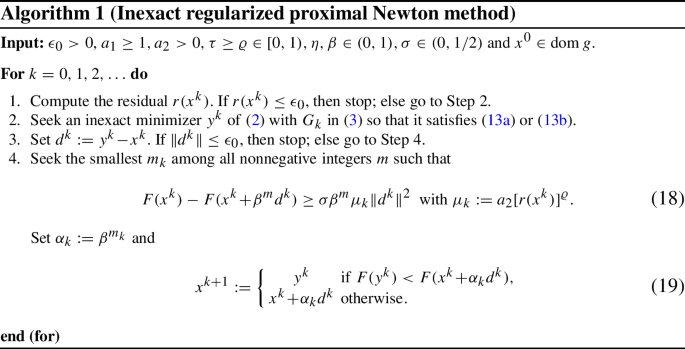
3 Inexact regularized proximal Newton method

Now we describe our inexact regularized proximal Newton method (IRPNM) for solving (1). Let $x^k$ be the current iterate. As mentioned previously, we adopt $G_k$ defined in (3) to construct the quadratic approximation model (2) at $x^k$. When $\psi$ is convex, this quadratic model reduces to the one used in [15, 23]. Since $G_k$ is positive definite, the objective function of (2) is strongly convex, so it has a unique minimizer, denoted by ${\overline{x}}^k$. For model (2), one may use the coordinate gradient descent method [7] as in [15] or the line search PG method as in [26] to seek an approximate minimizer $y^k$. Inspired by the structure of $G_k$, we develop in Sect. 5 a dual semismooth Newton augmented Lagrangian (SNALM) method to seek an approximate minimizer $y^k$.

To ensure that our IRPNM has a desirable convergence, we require $y^k$ to satisfy

where $\eta \in \!(0,1)$ and $\tau \!\ge \!\varrho$ are constants, and $r_k$ is the KKT residual of (2) given by

$$\begin{aligned} \begin{aligned} r_k(y)\!:=\!\Vert R_k(y)\Vert \ \ \text {with}\ R_k(y)\!:=y\!-\!{\mathcal {P}}_g(y\!- \!\nabla \!f(x^k)\!-\!G_k(y\!-\!x^k)) \quad {\text {for}}\ \ y\in {\mathbb {R}}^n. \end{aligned} \end{aligned}$$

(14)

Though the following inequality holds for $r_k(\cdot )$ and ${\textrm{dist}}(0,\partial \Theta _k(\cdot ))$ by [33, Lemma 4.1]

$$\begin{aligned} r_k(y)\le {\textrm{dist}}(0,\partial \Theta _k(y))\quad \hbox {for any}\quad y\in {\textrm{dom}}\,g, \end{aligned}$$

(15)

there is no direct relation between the first inequality of (13a) and that of (13b). Criterion (13a) is the same as the one used in [23], but is weaker than the one used in [15]. Indeed, let $\ell _k$ be the partial first-order approximation function of F at $x^k$:

$$\begin{aligned} \ell _k(x):=f(x^k)+\langle \nabla \!f(x^k),x\!-\!x^k\rangle +g(x)\quad \forall x\in {\mathbb {R}}^n. \end{aligned}$$

(16)

One can verify that $\Theta _k(y^k)-\Theta _k(x^k)\le 0$ if $\Theta _k(y^k)-\Theta _k(x^k)\le \zeta (\ell _k(y^k)-\ell _k(x^k))$ for some $\zeta \in (0,1)$ by using the positive definiteness of $G_k$ and the following relation

$$\begin{aligned} \Theta _k(x)-\Theta _k(x^k)=\ell _k(x)-\ell _k(x^k)+\frac{1}{2}(x-x^k)^{\top }G_k(x-x^k)\quad \ \forall x\in {\mathbb {R}}^n. \end{aligned}$$

(17)

As will be shown in Lemma 3 below, the vector $y^k$ satisfying (13b) is actually an exact minimizer of the canonical perturbation of (2). It seems that the distance involved in (13b) is difficult to compute in practice, but when choosing SNALM as the inner solver, one can easily achieve an element $\omega ^k\in \partial \Theta _k(y^k)$ (see Sect. 5.1.1) and then an upper bound $\Vert \omega ^k\Vert$ for ${\textrm{dist}}(0,\partial \Theta _k(y^k))$. Thus, the first inequality of criterion (13b) is guaranteed to hold by requiring $\Vert \omega ^k\Vert \le \eta r(x^k)$. It is worth pointing out that one can replace the first inequality in (13b) with $r_k(y^k)\le \eta r(x^k)$, but such $y^k$ become more inaccurate by (15), which will lead to more iterations and running time.

With an inexact minimizer $y^k$ of subproblem (2), we perform the Armijo line search along the direction $d^k:=y^k-x^k$ to capture a step-size $\alpha _k>0$ so that the objective value of problem (1) can gain a sufficient decrease. The algorithm steps into the next iterate with $x^{k+1}\!:=x^k\!+\!\alpha _kd^k$ if $F(x^k\!+\!\alpha _kd^k)<F(y^k)$, otherwise with $x^{k+1}\!:=y^k$. Now we are ready to summarize the iterate steps of our IRPNM.

Remark 3

• (a) Differently from the proximal Newton methods in [15, 23], the next iterate $x^{k+1}$ of Algorithm 1 may take $x^{k}+\alpha _kd^k$ or $y^k$, determined by their objective values. Note that a standard abstract convergence scheme adopted in the KL framework [32] usually requires a relative error condition at the iterates, while such a selection allows us to employ the relative error condition at $y^k$ (which might not be the next iterate) in the proof of convergence, which is crucial to achieve the global convergence of the iterate sequence $\{x^k\}_{k\in {\mathbb {N}}}$ for $\varrho =0$ under the KL property of F (see Theorem 4). To the best of our knowledge, such a technique first appears in [3, Algorithm 1].

• (b) The line search criterion in [15, Eq (7)] implies the one in Eq. (18). Indeed, equality (17) and $\Theta _k(y^k)\le \Theta _k(x^k)$ in criterion (13a) or (13b) implies that

  $$\begin{aligned} \ell _k(x^k)-\ell _k(y^k)\ge \frac{1}{2}\langle y^k-x^k,G_k(y^k\!-\!x^k)\rangle \ge \frac{1}{2}\mu _k\Vert y^k\!-\!x^k\Vert ^2. \end{aligned}$$

  (20)

  Since g is convex and $d^k=y^k\!-\!x^k$, for any $\tau \in [0,1]$ we have $x^k\!+\!\tau d^k\in {\textrm{dom}}\,g$ and $\ell _k(x^k)-\ell _k(x^k\!+\!\tau d^k)\ge \tau [\ell _k(x^k)-\ell _k(x^k\!+\!d^k)] =\tau [\ell _k(x^k)-\ell _k(y^k)]$, which by (20) implies that $\ell _k(x^k)-\ell _k(x^k\!+\!\tau d^k)\ge \frac{1}{2}\tau \mu _k\Vert y^k\!-\!x^k\Vert ^2$. Thus (18) holds. This implication suggests that (18) may need less computation time than the one in [15].

• (c) From (13a) or (13b) along with (15), for each $k\in {\mathbb {N}}$, $r_k(y^k)\le \eta r(x^k)$, and then

  $$\begin{aligned} (1\!-\!\eta )r(x^k)\le r(x^k)\!-\!r_k(y^k)\le 2\Vert d^k\Vert \!+\!\Vert G_k\Vert \Vert d^k\Vert , \end{aligned}$$

  (21)

  where the last inequality is using the expressions of $r(x^k)$ and $r_k(y^k)$. By the boundedness of $\{x^k\}_{k\in {\mathbb {N}}}$ (see Proposition 3 below) and the expression of $G_k$ in (3), we have $r(x^k)\le c_0\Vert d^k\Vert$ for some $c_0>0$. Thus, $d^k=0$ implies that $x^k$ is a stationary point of (1). This interprets why Algorithm 1 also adopts $\Vert d^k\Vert \le \epsilon _0$ as a termination condition.

• (d) When $H_k$ and $\eta _k$ in (S.1) of [26, Algorithm 3.1] take $G_k$ and $\eta \min \big \{1,[r(x^k)]^{\tau }\big \}$, respectively, under the unit step-size and the existence of ${\widehat{\kappa }}>0$ and ${\widetilde{k}}_0\in {\mathbb {N}}$ such that

  $$\begin{aligned} \begin{aligned} \Vert d^k\Vert \le {\widehat{\kappa }}[r(x^k)]^{{\widehat{q}}}\ \ ({\widehat{q}}>0)\quad \text {for\ all}\quad k\ge {\widetilde{k}}_0, \end{aligned} \end{aligned}$$

  (22)

  the sequence $\{x^k\}_{k\ge {\widetilde{k}}_0}$ generated by [26, Algorithm 3.1] is the same as the one yielded by Algorithm 1 with $\varrho \in (0,1)$. Indeed, using the same arguments as those for Lemma 3 below, one can show that the inexactness criterion in [26, Eq (13)] is well defined. In addition, by using Eq. (17), $G_k\succeq a_2[r(x^k)]^{\varrho }I$ and condition (22), it follows that

  $$\begin{aligned} 0&\ge \Theta _k(y^k)-\Theta _k(x^k) \ge \ell _k(y^k)-\ell _k(x^k) +(a_2/2)[r(x^k)]^{\varrho }\Vert d^k\Vert ^2\\&\ge \ell _k(y^k)-\ell _k(x^k)+(a_2/2){\widehat{\kappa }}^{-\frac{\varrho }{{\widehat{q}}}}\Vert d^k\Vert ^{2+\frac{\varrho }{{\widehat{q}}}}\quad \mathrm{for\ all}\quad k\ge {\widetilde{k}}_0. \end{aligned}$$

  This implies that [26, condition (14)] is satisfied with $\rho =\frac{1}{2}a_2{\widehat{\kappa }}^{-\frac{\varrho }{{\widehat{q}}}}$ and $p=2+{\varrho }/{{\widehat{q}}}$ when $k\ge {\widetilde{k}}_0$, so the iterates generated by [26, Algorithm 3.1] for $k\ge {\widetilde{k}}_0$ are the same as those yielded by Algorithm 1 with $\varrho \in (0,1)$. This fact, along with the convergence analysis in Sect. 4.2, shows that the global convergence and superlinear rate results of [26, Algorithm 3.1] there can be achieved under weaker conditions (see Remark 6).

• (e) A stepsize $t>0$ is generally introduced into the definition of KKT residual of (1) as $R_{t}(x)\!:=t^{-1}[x\!-\!{\mathcal {P}}_{tg}(x\!-\!t\nabla \!f(x))]$, and similarly a stepsize $t_k>0$ is done for the KKT residual of (2) as $R_{t_k}(x)\!:=t_k^{-1}[x\!-\!{\mathcal {P}}_{t_kg}(x\!-t_k(\nabla \!f(x^k)+G_k(x-\!x^k)))]$. In practice, one can search for $t_k$ via backtracking by the descent lemma (see Lemma 9). Concretely, with an initial lower estimate $L\!>0$ for the Lipschitz modulus of $\nabla \!f$ at $x^k$ and a ratio $\alpha >1$, the following if-end sentence can be added in step 1 before calculating $r(x^k)$:

If $f(z)\!>\!f(x^k)+\langle \nabla \!f(x^k),z-\!x^k\rangle \!+\!\frac{L}{2}\Vert z\!-\!x^k\Vert ^2$ for $z\!={\mathcal {P}}_{L^{-1}g}(x^k\!-\!L^{-1}\nabla \!f(x^k))$, then

   $L\leftarrow \alpha L$,

end if

and set $t_k:=1/L$. After testing Algorithm 1 with such KKT residuals, we found that it cannot improve the performance of Algorithm 1, and even requires more running time for some test examples. This phenomenon is reasonable by noting that our approximation matrix $G_k$ actually also plays the role of variable metric. Taking into account this, we simply take the unit stepsize for the functions r and $r_k$ throughout this paper.

Before analyzing the convergence of Algorithm 1, we need to verify that it is well defined, i.e., arguing that the inexactness conditions in (13a) and (13b) are feasible and the line search in (18) will terminate in a finite number of steps.

Lemma 3

For each iterate of Algorithm 1 with $\epsilon _0=0$, the criterion (13a) is satisfied by any $y\in {\textrm{dom}}\,g$ sufficiently close to the exact solution ${\overline{x}}^k$ of (2), the criterion (13b) is satisfied by $y_u:={\mathcal {P}}_g(y\!-\!\nabla f(x^k)-G_k(y\!-\!x^k))$ for any $y\in {\textrm{dom}}\,g$ sufficiently close to ${\overline{x}}^k$, and there is an integer $m_k\ge 0$ such that the descent condition (18) is satisfied.

Proof

Consider the iterate $x^k$. Assume that $x^k$ is not a stationary point of (1), i.e., $r_k(x^k)>0$. From the continuity of $r_k$ and $r_k({\overline{x}}^k)=0$, for any y sufficiently close to ${\overline{x}}^k$, $r_k(y)\le \eta \min \{r(x^k),[r(x^k)]^{1+\tau }\}$. In addition, since ${\overline{x}}^k$ is the unique optimal solution of (2), $G_k(x^k\!-\!{\overline{x}}^k)\in \partial \ell _k({\overline{x}}^k)$. This implies that $x^k\ne {\overline{x}}^k$ (if not, $0\in \partial \ell _k(x^k)$ and $x^k$ is a stationary point of (1)). By the convexity of $\ell _k$, $\ell _k(x^k)\ge \ell _k({\overline{x}}^k) +\langle G_k(x^k\!-\!{\overline{x}}^k),x^k\!-\!{\overline{x}}^k\rangle$, which along with (17) implies that

$$\begin{aligned} \Theta _k({\overline{x}}^k)-\Theta _k(x^k)&=\ell _k({\overline{x}}^k)-\ell _k(x^k) +(1/2)\langle x^k\!-\!{\overline{x}}^k,G_k(x^k\!-\!{\overline{x}}^k)\rangle \\&\le -(1/2)\langle x^k\!-\!{\overline{x}}^k,G_k(x^k\!-\!{\overline{x}}^k)\rangle \le -(1/2)\mu _k\Vert x^k\!-\!{\overline{x}}^k\Vert ^2<0. \end{aligned}$$

Since $\Theta _k$ is continuous relative to ${\textrm{dom}}\,g$ by Assumption 1 (ii), the last inequality means that for any $y\in {\textrm{dom}}\,g$ sufficiently close to ${\overline{x}}^k$, $\Theta _k(y)\le \Theta _k(x^k)$. The two sides show that criterion (13a) is satisfied by any $y\in {\textrm{dom}}\,g$ sufficiently close to ${\overline{x}}^k$.

For the first condition in (13b), consider problems (5) and (6) with $\vartheta$ given by

$$\begin{aligned} \vartheta (x)\!:=f(x^k)+\langle \nabla \!f(x^k),x-x^k\rangle +\frac{1}{2}(x-x^k)^{\top }G_k(x-x^k)\quad {\textrm{for}}\quad x\in {\mathbb {R}}^n. \end{aligned}$$

Let $R_{\vartheta }(x)\!=x-\!{\mathcal {P}}_g(x-\!\nabla \vartheta (x))$ be as in Proposition 1. Since ${\overline{x}}^k\!={\mathcal {P}}_g({\overline{x}}^k\!-\!\nabla \vartheta ({\overline{x}}^k))$, by the continuity of $\nabla \vartheta$, for any $y\in {\textrm{dom}}\,g$ sufficiently close to ${\overline{x}}^k$,

$$\begin{aligned} \Vert R_{\vartheta }(y)+\!\nabla \vartheta ({\mathcal {P}}_g(y-\!\nabla \vartheta (y))) -\!\nabla \vartheta (y)\Vert \le \eta \min \big \{r(x^k),[r(x^k)]^{1+\tau }\big \}. \end{aligned}$$

With such y, by Proposition 1 for ${\widehat{x}}=y$ and $u=R_{\vartheta }(y)+\!\nabla \vartheta ({\mathcal {P}}_g(y-\!\nabla \vartheta (y)))-\!\nabla \vartheta (y)$, it follows that ${\textrm{dist}}(0,\partial \Theta _k(y_{u}))\!\le \!\Vert u\Vert \! \le \!\eta \min \{r(x^k),[r(x^k)]^{1+\tau }\}$. In addition, from the above discussions, the second condition in (13b) hold for any $z\in {\textrm{dom}}\,g$ sufficiently close to ${\overline{x}}^k$. Note that $y_{u}\in {\textrm{dom}}\,g$ and $y_u$ is close to ${\overline{x}}^k$ as y is sufficiently close to ${\overline{x}}^k$. These two sides demonstrate that $y_u$ satisfies the criterion (13b) for any $y\in {\textrm{dom}}\,g$ sufficiently close to ${\overline{x}}^k$.

For the last part, we only need to consider that $d^k\ne 0$. From the convexity of g and the definition of directional derivative, it follows that

$$\begin{aligned} F'(x^k;d^k)&=\langle \nabla \!f(x^k),d^k\rangle +g'(x^k;d^k) \le \!\langle \nabla \!f(x^k),d^k\rangle +\!g(y^k)\!-\!g(x^k)\\&=\ell _k(y^k)-\ell _k(x^k)\le -({\mu _k}/{2})\Vert y^k\!-\!x^k\Vert ^2 =-({\mu _k}/{2})\Vert d^k\Vert ^2<0, \end{aligned}$$

where the first inequality is using [43, Theorem 23.1] and $d^k=y^k-x^k$, and the second inequality is using (20). Together with the definition of directional derivative,

$$\begin{aligned} F(x^k\!+\!t d^k)-F(x^k)\le -t\big [({\mu _k}/{2})\Vert d^k\Vert ^2-o(t)\big ]. \end{aligned}$$

This implies that the line search step in (18) is well defined. $\square$

To close this section, we summarize some properties of the sequence $\{x^k\}_{k\in {\mathbb {N}}}$.

Proposition 3

Let $\{x^k\}_{k\in {\mathbb {N}}}$ be a sequence generated by Algorithm 1 with $\epsilon _0=0$, and denote by $\omega (x^0)$ its cluster point set. Then, the following statements are true.

• (i) The sequence $\{F(x^k)\}_{k\in {\mathbb {N}}}$ is nonincreasing and convergent;

• (ii) The sequence $\{x^k\}_{k\in {\mathbb {N}}}$ is bounded;

• (iii) $\lim _{k\rightarrow \infty }r(x^k)=0$ and $\lim _{k\rightarrow \infty }\Vert d^k\Vert =0$;

• (iv) $\omega (x^0)\subset {\mathcal {S}}^*$ is a nonempty compact set and $F\equiv {\overline{F}}\!:={\displaystyle \lim _{k\rightarrow \infty }}F(x^k)$ on $\omega (x^0)$.

Proof

(i)–(ii) For each $k\in {\mathbb {N}}$, from (18) and (19), we have $F(x^{k+1})<F(x^k)$ and then $\{x^k\}_{k\in {\mathbb {N}}}\subset {\mathcal {L}}_{F}(x^0)\!:=\!\{x\in {\textrm{dom}}\,g\ |\ F(x)\le F(x^0)\}$. Since Assumption 1 (iii) implies that F is lower bounded and ${\mathcal {L}}_{F}(x^0)$ is bounded, we get parts (i) and (ii).

(iii) For each $k\in {\mathbb {N}}$, let $u^k\!=x^k\!-{\mathcal {P}}_g(x^k\!-\nabla \!f(x^k))$. Then $u^k\!-\!\nabla \!f(x^k)\in \partial g(x^k\!-\!u^k)$. By the expression of $R_k$, $R_k(y^k)\!-\!\nabla \!f(x^k)\!-\!G_k(y^k\!-\!x^k)\in \partial g(y^k\!-\!R_k(y^k))$. Using the monotonicity of $\partial g$, we have $\langle R_k(y^k)-G_kd^k-u^k,d^k-R_k(y^k)+u^k\rangle \ge 0$ or

$$\begin{aligned} \langle d^k,G_kd^k\rangle \le \langle R_k(y^k)\!-\!u^k,d^k\!-\!R_k(y^k)+u^k\!+\!G_kd^k\rangle \le \langle (I+G_k)d^k,R_k(y^k)\!-\!u^k\rangle . \end{aligned}$$

From the expression of $G_k$ in (3) and $\mu _k=a_2[r(x^k)]^{\varrho }$, $G_k\succeq \mu _kI$, which together with the last inequality and the expression of $R_k(y^k)$ implies that

$$\begin{aligned} a_2r(x^k)^{\varrho }\Vert d^k\Vert ^2\le (r_k(y^k)+r(x^k))(1\!+\!\Vert G_k\Vert )\Vert d^k\Vert \le (1\!+\!\eta )(1\!+\!\Vert G_k\Vert )r(x^k)\Vert d^k\Vert , \end{aligned}$$

where the last inequality is using $r_k(y^k)\le \eta r(x^k)$ obtained in Remark 3 (c). Then,

$$\begin{aligned} \Vert d^k\Vert \le a_2^{-1}(1+\eta )(1+\Vert G_k\Vert )r(x^k)^{1-\varrho } \quad \hbox {for each}\quad k\in {\mathbb {N}}. \end{aligned}$$

(23)

By part (ii) and the continuity of r, there exists a constant ${\widehat{\tau }}>0$ such that $\Vert d^k\Vert \le {\widehat{\tau }}$ for all $k\in {\mathbb {N}}$. Let ${\mathbb {B}}$ denote the unit ball of ${\mathbb {R}}^n$ centered at the origin. Assumption 1 (i) implies that $\nabla \!f$ is Lipschitz continuous on the compact set ${\mathcal {L}}_F(x^0)+{\widehat{\tau }}{\mathbb {B}}$, so there exists $L_{\nabla \!f}>0$ such that for any $x',x\in {\mathcal {L}}_F(x^0)+{\widehat{\tau }}{\mathbb {B}}$,

$$\begin{aligned} \Vert \nabla \!f(x)-\nabla \!f(x')\Vert \le L_{\nabla \!f}\Vert x-x'\Vert . \end{aligned}$$

(24)

Let ${\mathcal {K}}\!:=\{k\in {\mathbb {N}}\ |\ \alpha _k<1\}$. Fix any $k\in {\mathcal {K}}$. Since (18) is violated for the stepsize $t_k:=\alpha _k/\beta$, from the convexity of g and the definition of $\ell _k$, it follows that

$$\begin{aligned} \sigma \mu _k t_k\Vert d^k\Vert ^2&>f(x^k)-f(x^k+t_kd^k)+g(x^k)-g(x^k+t_kd^k) \nonumber \\&\ge f(x^k)-f(x^k+t_kd^k)+t_k(g(x^k)-g(y^k)) \nonumber \\&= f(x^k)-f(x^k+t_kd^k)+t_k(\langle \nabla \!f(x^k), d^k\rangle +\ell _k(x^k)-\ell _k(y^k))\nonumber \\&= t_k\langle \nabla \!f(x^k)-\nabla \!f(\xi ^k),d^k\rangle + t_k(\ell _k(x^k)-\ell _k(y^k)) \nonumber \\&\ge t_k\langle \nabla \!f(x^k)-\nabla \!f(\xi ^k),d^k\rangle + (t_k\mu _k/2)\Vert d^k\Vert ^2 \end{aligned}$$

(25)

for some $\xi ^k\in (x^k,x^k+t_kd^k)$, where the last equality is due to the mean-value theorem, and the last inequality comes from (20). Combining (25) and (24) leads to

$$\begin{aligned} (1/2\!-\!\sigma )t_k\mu _k\Vert d^k\Vert ^2\le t_k\Vert \nabla f(\xi ^k)\!-\!\nabla f(x^k)\Vert \Vert d^k\Vert \le L_{\nabla \!f}t_k^2\Vert d^k\Vert ^2, \end{aligned}$$

which implies that $t_k\ge \frac{1-2\sigma }{2L_{\nabla \!f}}\mu _k$. By the arbitrariness of $k\in {\mathcal {K}}$, $\alpha _k\ge \min \{1,\frac{1-2\sigma }{2L_{\nabla \!f}}\beta \mu _k\}$ for all $k\in {\mathbb {N}}$. While from (18) and part (i), $\lim _{k\rightarrow \infty }\alpha _k\mu _k\Vert d^k\Vert ^2=0$. Thus, $\lim _{k\rightarrow \infty }\min \big \{\mu _k,(1\!-\!2\sigma )\beta (2L_{\nabla \!f})^{-1}\mu _k^2\big \}\Vert d^k\Vert ^2=0$. Recall that $\Vert d^k\Vert \ge \frac{1-\eta }{2+\Vert G_k\Vert }r(x^k)$ by (21) and $\mu _k=a_2[r(x^k)]^{\varrho }$. The boundedness of $\{\Vert G_k\Vert \}$ then implies that $\lim _{k\rightarrow \infty }r(x^k)=0$. Together with (23), it follows that $\lim _{k\rightarrow \infty }\Vert d^k\Vert =0$.

(iv) By part (ii), the set $\omega (x^0)$ is nonempty and compact. Pick any ${\overline{x}}\in \omega (x^0)$. There is an index set ${\mathcal {K}}\subset {\mathbb {N}}$ such that $\lim _{{\mathcal {K}}\ni k\rightarrow \infty }x^{k}={\overline{x}}$. From part (iii) and the continuity of r, we have ${\overline{x}}\in {\mathcal {S}}^*$, and then $\omega (x^0)\subset {\mathcal {S}}^*$. Note that $\{x^k\}_{k\in {\mathcal {K}}}\subset {\textrm{dom}}\,g$ and F is continuous relative to ${\textrm{dom}}\,g$ by Assumption 1 (i)–(ii). Then, $F({\overline{x}})={\overline{F}}$, which shows that F is constant on the set $\omega (x^0)$. $\square$

4 Convergence analysis of Algorithm 1

This section focuses on the asymptotic convergence behaviour of Algorithm 1. To this end, we assume that the sequence $\{x^k\}_{k\in {\mathbb {N}}}$ is generated by Algorithm 1 with $\epsilon _0=0$.

4.1 Convergence analysis for $\varrho =0$

First, by using the first condition in (13b), we bound ${\textrm{dist}}(0,\partial F(y^k))$ in terms of $\Vert d^k\Vert$.

Lemma 4

For each $k\in {\mathbb {N}}$, there exists $w^k\in \partial F(y^k)$ with $\Vert w^k\Vert \le \gamma _0\Vert d^k\Vert$ for $\gamma _0\!=L_{\nabla \!f}\!+{\widetilde{\gamma }}+{\eta (2\!+\!{\widetilde{\gamma }})}/{(1\!-\!\eta )}$, where ${\widetilde{\gamma }}=L_{\nabla \!f}+a_1c_{\psi }\Vert A\Vert ^2+a_2$ with $c_{\psi }\!:=\max _{x\in {\mathcal {L}}_{F}(x^0)}[-\lambda _{\textrm{min}}(\nabla ^2\psi (Ax\!-\!b))]_{+}$, and $L_{\nabla \!f}$ is the constant appearing in (24).

Proof

Fix any $k\in {\mathbb {N}}$. Since ${\textrm{dist}}(0,\partial \Theta _k(y^k))\le \eta r(x^k)$ by (13b), there exists $\xi ^k\in \partial \Theta _k(y^k)$ with $\Vert \xi ^k\Vert \le \eta r(x^k)$. Let $w^k\!:=\xi ^k\!+\!\nabla \!f(y^k)\!-\!\nabla \!f(x^k)-G_k(y^k\!-\!x^k)$. From $\xi ^k\in \partial \Theta _k(y^k)$, we have $w^k\in \partial F(y^k)$. By the expression of $w^k$ and (24), it holds that

$$\begin{aligned} \Vert w^k\Vert&\le \Vert G_k(x^k\!-\!y^k)\Vert +\Vert \xi ^k+\nabla \!f(y^k)\!-\!\nabla \!f(x^k)\Vert \nonumber \\&\le \big [\Vert G_k\Vert +L_{\nabla \!f}\big ]\Vert d^k\Vert +\eta r(x^k). \end{aligned}$$

(26)

From the expression of $G_k$ for $\varrho =0$ and (24), it follows that $\Vert G_k\Vert \le {\widetilde{\gamma }}$. Together with (21), $r(x^k)\le (1-\eta )^{-1}(2+{\widetilde{\gamma }})\Vert d^k\Vert$. The desired result then follows by (26). $\square$

With Lemma 4, the following theorem establishes the convergence of the sequence $\{x^k\}_{k\in {\mathbb {N}}}$ under the KL assumption on F. Due to the selection scheme in (19), the analysis technique is a little different from the common one adopted in [31, 32].

Theorem 4

If F is a KL function, then $\sum _{k=0}^{\infty }\Vert x^{k+1}\!-\!x^k\Vert <\infty$ and hence the sequence $\{x^k\}_{k\in {\mathbb {N}}}$ is convergent with limit being a stationary point of (1).

Proof

If there exists ${\overline{k}}_1\in {\mathbb {N}}$ such that $F(x^{{\overline{k}}_1})=F(x^{{{\overline{k}}_1}+1})$, we have $d^{{\overline{k}}_1}=0$ by step 4, and Algorithm 1 stops within a finite number of steps. In this case, $r(x^{{\overline{k}}_1})=0$ follows from (21), i.e., $x^{{\overline{k}}_1}$ is a stationary point of (1). Hence, it suffices to consider that $F(x^k)>F(x^{k+1})$ for all $k\in {\mathbb {N}}$. By invoking Eq. (19), for each $k\in {\mathbb {N}}$,

$$\begin{aligned} F(y^k)-{\overline{F}}\ge F(x^{k+1})-{\overline{F}}>0, \end{aligned}$$

(27)

where ${\overline{F}}$ is the same as in Proposition 3 (iv). By Proposition 3 (iv), the set $\omega (x^0)$ is nonempty and compact, and $F\equiv {\overline{F}}$ on the set $\omega (x^0)$. Since F is assumed to be a KL function, by invoking [44, Lemma 6], there exist $\varepsilon>0,\varpi >0$ and $\varphi \in \Upsilon _{\!\varpi }$ such that for all $y\in [{\overline{F}}\!<F<{\overline{F}}+\varpi ]\cap {\mathfrak {B}}(\omega (x^0),\varepsilon )$ with ${\mathfrak {B}}(\omega (x^0),\varepsilon ) \!:=\!\{y\in {\mathbb {R}}^n\ |\ {\textrm{dist}}(y,\omega (x^0))\le \varepsilon \}$,

$$\begin{aligned} \varphi '(F(y)-{\overline{F}}){\textrm{dist}}(0,\partial F(y)) \ge 1. \end{aligned}$$

By Proposition 3 (iii) and $d^k=y^k-x^k$, $\lim _{k\rightarrow \infty }\Vert y^k-x^k\Vert =0$. Together with $\lim _{k\rightarrow \infty }{\textrm{dist}}(x^k,\omega (x^0))=0$, we have $\lim _{k\rightarrow \infty } {\textrm{dist}}(y^k,\omega (x^0))=0$. Obviously, $\{y^k\}_{k\in {\mathbb {N}}}$ is bounded, which along with $\{y^k\}_{k\in {\mathbb {N}}}\subset {\textrm{dom}}\,g$ and Assumption 1(i)–(ii) implies that $\{F(y^k)\}_{k\in {\mathbb {N}}}$ is bounded. We claim that $\lim _{k\rightarrow \infty }F(y^k)={\overline{F}}$. If not, by (27) there must exist an index set ${\mathcal {K}}\subset {\mathbb {N}}$ such that $\lim _{{\mathcal {K}}\ni k\rightarrow \infty }F(y^k)>{\overline{F}}$. Since $\{y^k\}_{k\in {\mathcal {K}}}$ is bounded, there exists an index set ${\mathcal {K}}_1\subset {\mathcal {K}}$ such that $\lim _{{\mathcal {K}}_1\ni k\rightarrow \infty }y^k=y^*$, which along with $\lim _{k\rightarrow \infty }\Vert d^k\Vert =0$ yields that $y^*\in \omega (x^0)$. Thus, from the continuity of F relative to ${\textrm{dom}}\,g$, $\lim _{{\mathcal {K}}\ni k\rightarrow \infty }F(y^k)=\lim _{{\mathcal {K}}_1\ni k\rightarrow \infty }F(y^k)=F(y^*)={\overline{F}}$, a contradiction to $\lim _{{\mathcal {K}}\ni k\rightarrow \infty }F(y^k)>{\overline{F}}$. Thus, the claimed limit $\lim _{k\rightarrow \infty }F(y^k)={\overline{F}}$ holds. Then, there exists ${\overline{k}}\in {\mathbb {N}}$ such that for all $k\ge {\overline{k}}$, $y^k\in {\mathfrak {B}}(\omega (x^0),\varepsilon )\cap [{\overline{F}}<F<{\overline{F}}+\varpi ]$, and hence $\varphi '\big (F(y^k)\!-\!{\overline{F}}\big ){\textrm{dist}}(0,\partial F(y^k))\ge 1$. By Lemma 4, for each $k\in {\mathbb {N}}$, there exists $w^k\in \partial F(y^{k})$ with $\Vert w^k\Vert \le \gamma _0\Vert d^k\Vert$. Consequently, for each $k\ge {\widehat{k}}:={\overline{k}}+1$,

$$\begin{aligned} \varphi '\big (F(y^{k-1})-{\overline{F}}\big )\Vert w^{k-1}\Vert \ge 1. \end{aligned}$$

(28)

In addition, from the proof of Proposition 3 (iii), $\alpha _k\mu _k\ge a_2\min (1,\frac{(1-2\sigma )\beta a_2}{2L_{\nabla \!f}})\!:={\underline{\alpha }}$ for each $k\in {\mathbb {N}}$, which along with (18)–(19) implies that for each $k\in {\mathbb {N}}$,

$$\begin{aligned} F(x^k)-F(x^{k+1})\ge \sigma {\underline{\alpha }}\Vert d^k\Vert ^2 =\sigma {\underline{\alpha }}\Vert y^k-x^k\Vert ^2. \end{aligned}$$

(29)

Fix any $k\ge {\widehat{k}}$. Since $\varphi '$ is nonincreasing on $(0,\varpi )$ by the concavity of $\varphi$, combining (27) with (28) and using $\Vert w^{k-1}\Vert \le \gamma _0\Vert d^{k-1}\Vert$ yields that

$$\begin{aligned} \varphi '(F(x^k)\!-\!{\overline{F}})\ge \varphi '(F(y^{k-1})\!-\!{\overline{F}}) \ge \frac{1}{\Vert w^{k-1}\Vert }\ge \frac{1}{\gamma _0\Vert y^{k-1}\!-\!x^{k-1}\Vert }. \end{aligned}$$

(30)

Together with the concavity of $\varphi$ and inequality (29), it follows that

$$\begin{aligned} \Delta _{k,k+1}&:=\varphi (F(x^k)\!-\!{\overline{F}})-\varphi (F(x^{k+1})\!-\!{\overline{F}}) \ge \varphi '(F(x^k)-{\overline{F}})(F(x^{k})\!-\!F(x^{k+1}))\\&\ge \frac{F(x^{k})\!-\!F(x^{k+1})}{\gamma _0\Vert y^{k-1}-x^{k-1}\Vert } \ge \frac{\sigma {\underline{\alpha }}\Vert y^k-x^k\Vert ^2}{\gamma _0\Vert y^{k-1}-x^{k-1}\Vert }. \end{aligned}$$

Then, $\Vert y^k\!-\!x^k\Vert \le \sqrt{\frac{\gamma _0}{\sigma {\underline{\alpha }}}\Delta _{k,k+1}\Vert y^{k-1}\!-\!x^{k-1}\Vert }$. From $2\sqrt{ts}\le t+s$ for $t\ge 0,s\ge 0$,

$$\begin{aligned} 2\Vert y^k\!-\!x^k\Vert \le \gamma _0(\sigma {\underline{\alpha }})^{-1}\Delta _{k,k+1}+\Vert y^{k-1}\!-\!x^{k-1}\Vert . \end{aligned}$$

By summing this inequality from k to $l>k$, it is immediate to obtain that

$$\begin{aligned} 2{\textstyle \sum _{i=k}^l}\Vert y^i-x^i\Vert&\le {\textstyle \sum _{i=k}^l}\Vert y^{i-1}-x^{i-1}\Vert +\gamma _0(\sigma {\underline{\alpha }})^{-1}{\textstyle \sum _{i=k}^l}\Delta _{i,i+1}\\&\le {\textstyle \sum _{i=k}^l}\Vert y^i-x^i\Vert +\Vert y^{k-1}-x^{k-1}\Vert +\gamma _0(\sigma {\underline{\alpha }})^{-1}\varphi \big (F(x^{k})-{\overline{F}}\big ), \end{aligned}$$

where the second inequality is using the nonnegativity of $\varphi (F(x^{l+1})-{\overline{F}})$. Thus,

$$\begin{aligned} {\textstyle \sum _{i=k}^l}\Vert y^i-x^i\Vert \le \Vert y^{k-1}-x^{k-1}\Vert +\gamma _0(\sigma {\underline{\alpha }})^{-1}\varphi (F(x^{k})-{\overline{F}}). \end{aligned}$$

(31)

Passing the limit $l\rightarrow \infty$ to this inequality yields that $\sum _{i=k}^{\infty }\Vert y^i-x^i\Vert <\infty$. Note that $\Vert x^{i+1}-x^i\Vert \le \Vert y^i-x^i\Vert$ for each $i\in {\mathbb {N}}$. Then, $\sum _{i=0}^{\infty }\Vert x^{i+1}-x^i\Vert <\infty$. $\square$

Next we deduce the linear and sublinear convergence rates of the sequence $\{x^k\}_{k\in {\mathbb {N}}}$ under the KL property of the function F with exponent 1/(2q) for $q\in (1/2,1]$.

Theorem 5

If F is a KL function of exponent 1/(2q) with $q\in ({1}/{2},1]$, then the sequence $\{x^k\}_{k\in {\mathbb {N}}}$ converges to a point ${\overline{x}}\in {\mathcal {S}}^*$ and there exist constants $\gamma \in (0,1)$ and $c_1>0$ such that for all sufficiently large k,

$$\begin{aligned} \Vert x^k-{\overline{x}}\Vert \le \left\{ \begin{array}{ll} c_1\gamma ^{k} &{}\quad {\textrm{for}}\quad q=1,\\ c_1 k^{\frac{2q-1}{2(q-1)}}&{}\quad {\textrm{for}}\quad q\in ({1}/{2},1). \end{array}\right. \end{aligned}$$

Proof

For each $k\in {\mathbb {N}}$, write $\Delta _k\!:=\sum _{i=k}^{\infty }\Vert y^i-x^i\Vert$. Fix any $k\ge {\widehat{k}}$ where ${\widehat{k}}$ is the same as in the proof of Theorem 4. From inequality (31), it follows that

$$\begin{aligned} \Delta _k\le \Vert y^{k-1}\!-\!x^{k-1}\Vert +\gamma _0(\sigma {\underline{\alpha }})^{-1}\varphi (F(x^{k})-{\overline{F}}) \end{aligned}$$

where $\varphi (t)=ct^{\frac{2q-1}{2q}}\ (t>0)$ for some $c>0$. From the expression of $\varphi$ and (30), $(F(x^{k})\!-\!{\overline{F}})^{\frac{1}{2q}}\le c(1\!-\!0.5/q)\gamma _0\Vert y^{k-1}\!-\!x^{k-1}\Vert$. Together with the last inequality,

$$\begin{aligned} \Delta _k&\le \Vert y^{k-1}\!-\!x^{k-1}\Vert +\frac{c\gamma _0}{\sigma {\underline{\alpha }}} \Big [\frac{c(2q\!-\!1)\gamma _0}{2q}\Big ]^{2q-1}\Vert y^{k-1}\!-\!x^{k-1}\Vert ^{2q-1}\\&\le \Vert y^{k-1}\!-\!x^{k-1}\Vert ^{2q-1}+\frac{(c\gamma _0)^{2q}}{\sigma {\underline{\alpha }}} \Big [\frac{(2q\!-\!1)}{2q}\Big ]^{2q-1}\Vert y^{k-1}\!-\!x^{k-1}\Vert ^{2q-1}\\&=\gamma _1(\Delta _{k-1}\!-\!\Delta _k)^{2q-1}\ \ \textrm{with}\ \ \gamma _1=\Big [1+\frac{(c\gamma _0)^{2q}}{\sigma {\underline{\alpha }}} \Big (\frac{(2q\!-\!1)}{2q}\Big )^{2q-1}\Big ], \end{aligned}$$

where the second inequality is due to $\lim _{k\rightarrow \infty }\Vert d^k\Vert =0$. When $q=1$, $\Delta _k\le \frac{\gamma _1}{1+\gamma _1}\Delta _{k-1}$. From this recursion formula, it follows that $\Delta _k\le (\frac{\gamma _1}{1+\gamma _1})^{k-{\widehat{k}}}\Delta _{{\widehat{k}}}$. Note that $\Vert x^k-{\overline{x}}\Vert \le \sum _{i=k}^{\infty }\Vert x^{i+1}-x^i\Vert \le \sum _{i=k}^{\infty }\Vert y^i-x^i\Vert =\Delta _k$. The conclusion holds with $\gamma ={\gamma _1}/{(1+\!\gamma _1)}$ and $c_1=\Delta _{{\widehat{k}}}(\frac{\gamma _1}{1+\gamma _1})^{-{\widehat{k}}}$. When $q\in (1/2,1)$, from the last inequality, we have $\Delta _k^{\frac{1}{2q-1}}\le (\gamma _1)^{\frac{1}{2q-1}}(\Delta _{k-1}\!-\!\Delta _k)$ for all $k\ge {\widehat{k}}$. By using this inequality and following the same analysis technique as those in [45, Page 14], we obtain $\Delta _{k}\le c_1k^{\frac{2q-1}{2(q-1)}}$ for some $c_1>0$. Consequently, $\Vert x^k-{\overline{x}}\Vert \le c_1k^{\frac{2q-1}{2(q-1)}}$ for all $k\ge {\widehat{k}}$. $\square$

Remark 4

The linear and sublinear convergence rates of the objective value sequence $\{F(x^k)\}_{k\in {\mathbb {N}}}$ can also be obtained under the assumption of Theorem 5. Indeed, let $\Delta _k=F(x^k)-{\overline{F}}$ for each $k\in {\mathbb {N}}$. Fix any $k\ge {\widehat{k}}$ where ${\widehat{k}}$ is the same as in the proof of Theorem 4. From inequality (30) with $\varphi (t)=ct^{(2q-1)/(2q)}$ and (29), it follows that

$$\begin{aligned} \Delta _k^{\frac{1}{q}}\le \frac{[c\gamma _0(2q-1)]^2}{4q^2}\Vert d^{k-1}\Vert ^2\le \gamma _1(\Delta _{k-1}-\Delta _k)\quad \textrm{with}\quad \gamma _1=\frac{[c\gamma _0(2q-1)]^2}{4q^2{\underline{\alpha }}\sigma }. \end{aligned}$$

When $q=1$, $\Delta _k\le \frac{\gamma _1}{1+\gamma _1}\Delta _{k-1}$ for all $k\ge {\widehat{k}}$. This implies that $\{F(x^k)\}_{k\in {\mathbb {N}}}$ converges to ${\overline{F}}$ with Q-linear rate. When $q\in (1/2,1)$, we have $\Delta _k^{1/q}\le \gamma _1(\Delta _{k-1}-\Delta _k)$ for all $k\ge {\widehat{k}}$. By using this inequality and following the same analysis technique as those in [45, Page 14], there exists $c_1>0$ such that $F(x^k)-{\overline{F}}\le c_1k^{-q/(1-q)}$ for all $k\ge {\widehat{k}}$.

4.2 Convergence analysis for $0<\varrho <1$

To analyze the global convergence of the sequence $\{x^k\}_{k\in {\mathbb {N}}}$ and its superlinear rate in this scenario, we need several technical lemmas. First, by noting that $G_k(x^k\!-\!{\overline{x}}^k)\!-\!\nabla \!f(x^k)\in \partial g({\overline{x}}^k)$ and $R_k(y^k)\!-\!\nabla \!f(x^k)-G_k(y^k\!-\!x^k)\in \partial g(y^k\!-\!R_k(y^k))$ for each $k\in {\mathbb {N}}$, using the monotonicity of $\partial g$ and $G_k\succeq \mu _kI$ can bound the error between $y^k$ and ${\overline{x}}^k$.

Lemma 5

For each $k\in \!{\mathbb {N}}$, it holds that $\Vert y^k\!-{\overline{x}}^k\Vert \!\le a_2^{-1}\eta (1+\Vert G_k\Vert )[r(x^k)]^{1+\tau -\varrho }.$

The following lemma bounds the distance from $x^k$ to the exact minimizer ${\overline{x}}^k$ of (2) by ${\textrm{dist}}(x^k,{\mathcal {S}}^*)$, which extends the result of [15, Lemma 4] to the nonconvex setting.

Lemma 6

Consider any ${\overline{x}}\in \omega (x^0)$. Suppose that $\nabla ^2\psi$ is strictly continuous at $A{\overline{x}}-b$ relative to $A({\textrm{dom}}\,g)-b$. Then, there exist $\varepsilon _0>0$ and $L_{\psi }>0$ such that for all $x^k\in {\mathbb {B}}({\overline{x}},{\varepsilon _0}/{2})$, $\Vert x^k\!-\!{\overline{x}}^k\Vert \le \big ((0.5L_{\psi }/\mu _k)\Vert A\Vert ^3{\textrm{dist}}(x^k,{\mathcal {S}}^*)+(\Lambda _k/\mu _k)\Vert A\Vert ^2+2\big ){\textrm{dist}}(x^k,{\mathcal {S}}^*)$, where $\Lambda _k\!:=a_1[-\lambda _{\textrm{min}}(\nabla ^2\psi (Ax^k\!-\!b))]_{+}$.

Proof

Since $\nabla ^2\psi$ is strictly continuous at $A{\overline{x}}-b$ relative to $A({\textrm{dom}}\,g)-b$, there exist $\delta _0>0$ and $L_{\psi }>0$ such that for any $z,z'\in {\mathbb {B}}(A{\overline{x}}-b,\delta _0)\cap [A({\textrm{dom}}\,g)-b]$,

$$\begin{aligned} \Vert \nabla ^2\psi (z)\!-\!\nabla ^2\psi (z')\Vert \le L_{\psi }\Vert z-z'\Vert . \end{aligned}$$

(32)

Take $\varepsilon _0={\delta _0}/{\Vert A\Vert }$. For any $x,x'\in {\mathbb {B}}({\overline{x}},\varepsilon _0)\cap {\textrm{dom}}\,g$, we have $Ax\!-\!b,Ax'\!-\!b\in {\mathbb {B}}(A{\overline{x}}\!-\!b,\delta _0)\cap [A({\textrm{dom}}\,g)\!-\!b]$, which together with $\nabla ^2\!f(\cdot )=A^{\top }\nabla ^2\psi (A\cdot \!-b)A$ implies that

$$\begin{aligned} \Vert \nabla ^2\!f(x)\!-\!\nabla ^2\!f(x')\Vert \le L_{\psi }\Vert A\Vert ^3\Vert x-x'\Vert . \end{aligned}$$

(33)

Fix any $x^k\in {\mathbb {B}}({\overline{x}},{\varepsilon _0}/{2})$. Pick any $x^{k,*}\!\in \Pi _{{\mathcal {S}}^*}(x^k)$. Since ${\overline{x}}\in {\mathcal {S}}^*$ by Proposition 3 (iv), we have $\Vert x^{k,*}-{\overline{x}}\Vert \le 2\Vert x^k-{\overline{x}}\Vert \le \varepsilon _0$, so $\Vert (1\!-\!t)x^k+\!t x^{k,*}\!-{\overline{x}}\Vert \le \varepsilon _0$ for all $t\in [0,1]$. Clearly, $(1-\!t)x^k\!+\!t x^{k,*}\in {\textrm{dom}}\,g$ for all $t\in [0,1]$ by the convexity of ${\textrm{dom}}\,g$. Thus, $(1-\!t)x^k\!+\!t x^{k,*}\in {\mathbb {B}}({\overline{x}},\varepsilon _0)\cap {\textrm{dom}}\,g$ for all $t\in [0,1]$. Note that $0\in \nabla \!f(x^{k,*})+\partial g(x^{k,*})$ and $0\in \nabla \!f(x^k)+G_k({\overline{x}}^k\!-\!x^k)+\partial g({\overline{x}}^k)$. From the monotonicity of $\partial g$, it follows that

$$\begin{aligned} 0\le \langle -\nabla \!f(x^{k,*})+\nabla \!f(x^k)+G_k(x^{k,*}\!-\!x^k), x^{k,*}\!-\!{\overline{x}}^k\rangle +\langle G_k({\overline{x}}^k\!-\!x^{k,*}),x^{k,*}\!-\!{\overline{x}}^k\rangle . \end{aligned}$$

Together with $G_k\succeq \mu _kI$ and the triangle inequality, we obtain that

$$\begin{aligned} \Vert {\overline{x}}^k-x^{k,*}\Vert&\le \mu _k^{-1}\Vert \nabla \!f(x^k)-\nabla \!f(x^{k,*})+G_k(x^{k,*}\!-\!x^k)\Vert \\&=\frac{1}{\mu _k}\Big \Vert \int _{0}^1\big [G_k\!-\!\nabla ^2\!f(x^{k}\!+\!t(x^{k,*}\!-\!x^k))\big ](x^{k,*}\!-\!x^k)dt\Big \Vert \\&\le \mu _k^{-1}\big [(L_{\psi }\Vert A\Vert ^3/2)\Vert x^{k,*}\!-\!x^k\Vert ^2 +\Lambda _k\Vert A\Vert ^2\Vert x^{k,*}\!-\!x^k\Vert \big ]\\&\quad +\Vert x^{k,*}\!-\!x^k\Vert , \end{aligned}$$

where the last inequality is using (33) with $x=x^k$ and $x'=x^{k}\!+\!t(x^{k,*}\!-\!x^k)$. The conclusion then follows by using $\Vert {\overline{x}}^k\!-\!x^k\Vert \le \Vert {\overline{x}}^k\!-\!x^{k,*}\Vert +\Vert x^{k,*}\!-\!x^k\Vert$. $\square$

The following lemma bounds $\Lambda _k$ defined in Lemma 6 in terms of ${\textrm{dist}}(x^k,{\mathcal {X}}^*)$. This result appeared early in [27, Lemma 5.2], and we here provide a concise proof.

Lemma 7

Consider any ${\overline{x}}\in {\mathcal {X}}^*$. Suppose that $\nabla ^2\psi$ is strictly continuous at $A{\overline{x}}-b$ relative to $A({\textrm{dom}}\,g)-b$. Then,

$$\begin{aligned} \Lambda _k\!\le \!a_1L_{\psi }\Vert A\Vert {\textrm{dist}}(x^k,{\mathcal {X}}^*)\quad \mathrm{for\ all}\ x^k\!\in {\mathbb {B}}({\overline{x}},{\varepsilon _0}/{2}) \end{aligned}$$

where $\varepsilon _0,\,L_{\psi }$ and $\Lambda _k$ are the same as those appearing in Lemma 6.

Proof

Fix any $x^k\in {\mathbb {B}}({\overline{x}},{\varepsilon _0}/{2})$. By the expression of $\Lambda _k$, it suffices to consider that $\lambda _{\textrm{min}}(\nabla ^2\psi (Ax^k\!-\!b))<0$. Pick any $x^{k,*}\in \Pi _{{\mathcal {X}}^*}(x^k)$. From ${\overline{x}}\in {\mathcal {X}}^*$, we have $\Vert x^{k,*}-{\overline{x}}\Vert \le 2\Vert x^k-{\overline{x}}\Vert \le \varepsilon _0$, and consequently $x^{k,*}\in {\mathbb {B}}({\overline{x}},\varepsilon _0)\cap {\textrm{dom}}\,g$. From $x^{k,*}\in {\mathcal {X}}^*$, we have $\nabla ^2\psi (Ax^{k,*}\!-\!b)\succeq 0$. When $\lambda _{\textrm{min}}(\nabla ^2\psi (Ax^{k,*}\!-\!b))=0$, it holds that

$$\begin{aligned} \Lambda _k&=-a_1\lambda _{\textrm{min}}(\nabla ^2\psi (Ax^k\!-\!b)) =a_1[\lambda _{\textrm{min}}(\nabla ^2\psi (Ax^{k,*}\!-\!b))-\lambda _{\textrm{min}}(\nabla ^2\psi (Ax^k\!-\!b))]\\&\le a_1\Vert \nabla ^2\psi (Ax^{k,*}\!-\!b)\!-\!\nabla ^2\psi (Ax^k\!-\!b)\Vert \le a_1L_{\psi }\Vert A\Vert \Vert x^k\!-\!x^{k,*}\Vert , \end{aligned}$$

where the first inequality is using the Lipschitz continuity of the function ${\mathbb {S}}^n\ni Z\mapsto \lambda _{\textrm{min}}(Z)$ with modulus 1, and the second one is using (32) with $Ax^{k,*}-b,Ax^k-b\in {\mathbb {B}}(A{\overline{x}}-b,\delta _0)\cap [A({\textrm{dom}}\,g)-b]$. So we only need to consider that $\lambda _{\textrm{min}}(\nabla ^2\psi (Ax^{k,*}\!-\!b))>0$. For this purpose, let $\phi _{k}(t):=\lambda _{\textrm{min}}[\nabla ^2\psi (Ax^k\!-\!b+\!tA(x^{k,*}\!-\!x^k))]$ for $t\ge 0$. Clearly, $\phi _{k}$ is continuous on any open interval containing [0, 1]. Note that $\phi _k(0)<0$ and $\phi _k(1)>0$. There exists ${\overline{t}}_k\in (0,1)$ such that $\phi _k({\overline{t}}_k)=0$. Consequently,

$$\begin{aligned} \Lambda _k&=a_1\big [\lambda _{\textrm{min}}(\nabla ^2\psi (Ax^k\!-\!b+{\overline{t}}_kA(x^{k,*}\!-\!x^k))) -\lambda _{\textrm{min}}(\nabla ^2\psi (Ax^k\!-\!b))\big ]\\&\le a_1\Vert \nabla ^2\psi (Ax^k\!-\!b+\!{\overline{t}}_kA(x^{k,*}\!-\!x^k))\!-\!\nabla ^2\psi (Ax^k\!-\!b)\Vert \le a_1L_{\psi }\Vert A\Vert \Vert x^{k,*}\!-\!x^k\Vert . \end{aligned}$$

This shows that the desired result holds. The proof is completed. $\square$

Remark 5

• (a) When ${\mathcal {X}}^*$ in Lemma 7 is replaced by ${\mathcal {S}}^*$, the conclusion may not hold. For example, consider problem (1) with $g\equiv 0$ and f given by Remark 2(a), and ${\overline{x}}=(0,0)^{\top }\!\in {\mathcal {S}}^*$. For each $k>1$, let $x^k=(0,\frac{1}{k})^{\top }$. We have $\Lambda _k=a_1(1\!-\!\frac{3}{k^2})$ but ${\textrm{dist}}(x^k,{\mathcal {S}}^*)\!=\frac{1}{k}$. Clearly, for all k large enough, $\Lambda _k\le a_1L{\textrm{dist}}(x^k,{\mathcal {S}}^*)$ does not hold.

• (b) The result of Lemma 7 may not hold if ${\textrm{dist}}(x^k,{\mathcal {X}}^*)$ is replaced by ${\textrm{dist}}(x^k,{\mathcal {S}}^*)$. Indeed, consider $f(x)=-(x-2)^{4}$ and $g(x)=\left\{ \begin{array}{cl} \infty &{} \textrm{if}\ x<0,\\ \!(x-2)^{4} &{} \textrm{if}\ x\ge 0 \end{array}\right.$ for $x\in {\mathbb {R}}$. We have ${\mathcal {S}}^*\!=\!{\mathbb {R}}_{+}$ and then ${\mathcal {X}}^*\!=\!\{2\}$. Let ${\overline{x}}=2$ and $x^k\!=2\!-\frac{1}{k}$. Then, $\Lambda _k\!=\frac{12a_1}{k^2}$, but ${\textrm{dist}}(x^k,{\mathcal {S}}^*)\!=0$. Clearly, $\Lambda _k\le a_1L{\textrm{dist}}(x^k,{\mathcal {S}}^*)$ does not hold for each $k\in {\mathbb {N}}$.

Next we show that the unit step-size must occur when the iterates are close enough to a cluster point and the following locally Hölderian error bound on ${\mathcal {X}}^*$ holds.

Assumption 3

The locally Hölderian error bound of order $q>0$ at any ${\overline{x}}\in \omega (x^0)$ on ${\mathcal {X}}^*$ holds, i.e., for any ${\overline{x}}\in \omega (x^0)$, there exist $\varepsilon >0$ and $\kappa >0$ such that for all $x\in {\mathbb {B}}({\overline{x}},\varepsilon )\cap {\textrm{dom}}\,g$, ${\textrm{dist}}(x,{\mathcal {X}}^*)\le \kappa [r(x)]^q$.

Lemma 8

Fix any ${\overline{x}}\in \omega (x^0)$. Suppose that $\nabla ^2\psi$ is strictly continuous at $A{\overline{x}}\!-\!b$ relative to $A({\textrm{dom}}\,g)\!-\!b$, and that Assumption 3 holds with $q>\varrho$. Then, there exists ${\overline{k}}\in {\mathbb {N}}$ such that $\alpha _k=1$ for all $x^k\in {\mathbb {B}}({\overline{x}},\varepsilon _1)$ with $k\ge {\overline{k}}$ and $\varepsilon _1=\min (\varepsilon ,{\varepsilon _0}/{2})$, where $\varepsilon$ and $\varepsilon _0$ are the same as in Assumption 3 and Lemma 6.

Proof

Since ${\overline{x}}\in \omega (x^0)$, there is ${\mathcal {K}}\subset {\mathbb {N}}$ such that $\lim _{{\mathcal {K}}\ni k\rightarrow \infty }x^k={\overline{x}}$, which by Assumption 3 and $\{x^k\}_{k\in {\mathbb {N}}}\!\subset {\textrm{dom}}\,g$ means that ${\textrm{dist}}(x^k,{\mathcal {X}}^*)\le \kappa [r(x^k)]^q$ for all $k\in {\mathcal {K}}$ large enough, so ${\overline{x}}\in {\mathcal {X}}^*$ follows by passing ${\mathcal {K}}\ni k\rightarrow \infty$ and using Proposition 3 (iii). Recall that $d^k=y^k-x^k$ for each $k\in {\mathbb {N}}$. By invoking Lemmas 5–7, for all $x^k\in {\mathbb {B}}({\overline{x}},\varepsilon _1)$,

$$\begin{aligned} \Vert d^k\Vert&\le \Vert y^k-{\overline{x}}^k\Vert +\Vert x^k-{\overline{x}}^k\Vert \le \frac{\eta (1\!+\!\Vert G_k\Vert )}{a_2}[r(x^k)]^{1+\tau -\varrho } \\&\quad \!+\!\big [0.5L_{\psi }\Vert A\Vert ^3\mu _k^{-1}{\textrm{dist}}(x^k,{\mathcal {S}}^*) \!\\&\quad +\!a_1L_{\psi }\Vert A\Vert ^2\mu _k^{-1}{\textrm{dist}}(x^k,{\mathcal {X}}^*)\!+\!2\big ]{\textrm{dist}}(x^k,{\mathcal {S}}^*). \end{aligned}$$

By Proposition 3(iv), for each $k\in {\mathbb {N}}$, ${\textrm{dist}}(x^k,{\mathcal {S}}^*)\le {\textrm{dist}}(x^k,\omega (x^0))$, which along with $\lim _{k\rightarrow \infty }{\textrm{dist}}(x^k,\omega (x^0))=0$ implies that for each $k\in {\mathbb {N}}$, $\Pi _{{\mathcal {S}}^*}(x^k)\subset {\mathcal {L}}_F(x^0)+{\widehat{\tau }}{\mathbb {B}}$ (if necessary by increasing ${\widehat{\tau }}$.) Thus, for each $k\in {\mathbb {N}}$, with any $x^{k,*}\in \Pi _{{\mathcal {S}}^*}(x^k)$, we have

$$\begin{aligned} r(x^k)= & {} \Vert x^k\!-\!{\mathcal {P}}_g(x^k\!-\!\nabla \!f(x^k))\!-\!x^{k,*} +{\mathcal {P}}_g(x^{k,*}\!-\!\nabla \!f(x^{k,*}))\Vert \nonumber \\{} & {} \le (2+L_{\nabla \!f}){\textrm{dist}}(x^k,{\mathcal {S}}^*). \end{aligned}$$

(34)

From ${\mathcal {X}}^*\subset {\mathcal {S}}^*$ and Assumption 3, for all $x^k\in {\mathbb {B}}({\overline{x}},\varepsilon _1)$, it holds that

$$\begin{aligned} \frac{1}{\mu _k}=\frac{1}{a_2}r(x^k)^{-\varrho }\le \frac{\kappa ^{\frac{\varrho }{q}}}{a_2}{\textrm{dist}}(x^k,{\mathcal {X}}^*)^{-\frac{\varrho }{q}}\le \frac{\kappa ^{\frac{\varrho }{q}}}{a_2}{\textrm{dist}}(x^k,{\mathcal {S}}^*)^{-\frac{\varrho }{q}}. \end{aligned}$$

(35)

In addition, from (34) and Assumption 3, it follows that for all $x^k\in {\mathbb {B}}({\overline{x}},\varepsilon _1)$,

$$\begin{aligned} \frac{{\textrm{dist}}(x^k,{\mathcal {X}}^*)}{\mu _k} \le \frac{\kappa }{a_2}r(x^k)^{q-\varrho } \le \frac{\kappa (2\!+L_{\nabla \!f})^{q-\varrho }}{a_2}{\textrm{dist}}(x^k,{\mathcal {S}}^*)^{q-\varrho }. \end{aligned}$$

From the last four inequalities, we deduce that for all $x^k\in {\mathbb {B}}({\overline{x}},\varepsilon _1)$,

$$\begin{aligned} \Vert d^k\Vert&\le \bigg [\frac{\eta (1\!+\!\Vert G_k\Vert )(2\!+\!L_{\nabla \!f})^{1+\tau -\varrho }}{a_2} [{\textrm{dist}}(x^k,{\mathcal {S}}^*)]^{\tau -\varrho }\nonumber \\&\quad +\frac{L_{\psi }\Vert A\Vert ^3\kappa ^{\frac{\varrho }{q}}}{2a_2}[{\textrm{dist}}(x^k,{\mathcal {S}}^*)]^{1-\frac{\varrho }{q}} \nonumber \\&\quad +\frac{\kappa a_1L_{\psi }\Vert A\Vert ^2(2\!+\!L_{\nabla \!f})^{q-\varrho }}{a_2} [{\textrm{dist}}(x^k,{\mathcal {S}}^*)]^{q-\varrho }+2\bigg ]{\textrm{dist}}(x^k,{\mathcal {S}}^*). \end{aligned}$$

(36)

From (35)–(36), the boundedness of $\{G_k\}$, and $\lim _{k\rightarrow \infty }{\textrm{dist}}(x^k,{\mathcal {S}}^*)=0$ by Proposition 3 (iv), we conclude that $[(1-2\sigma )\mu _k]^{-1}\Vert d^k\Vert \le O({\textrm{dist}}(x^k,S^*)^{1-\frac{\varrho }{q}})$. Along with $q>\varrho$, there exists ${\overline{k}}\in {\mathbb {N}}$ such that for all $k\ge {\overline{k}}$, when $x^k\in {\mathbb {B}}({\overline{x}},\varepsilon _1)$, $\frac{\Vert d^k\Vert }{(1-2\sigma )\mu _k}\le \frac{3}{L_{\psi }\Vert A\Vert ^3}$ and $x^k+t d^k\in {\mathbb {B}}({\overline{x}},\varepsilon _0)$ for all $t\in [0,1]$. Fix any integer $m\ge 0$. By using (33),

$$\begin{aligned}&f(x^k\!+\!\beta ^md^k)\!-\!f(x^k)\\&\quad =\int _{0}^{1}\beta ^m\langle [\nabla \!f(x^k\!+\!t\beta ^md^k)-\nabla \!f(x^k)],d^k\rangle dt +\beta ^m\langle \nabla \!f(x^k),d^k\rangle \\&\quad =\int _{0}^{1}\int _{0}^{1}t\beta ^{2m}\langle d^k,[\nabla ^2\!f(x^k\!+\!st\beta ^md^k) \!-\!\nabla ^2\!f(x^k)]d^k\rangle dsdt\\&\qquad +\int _{0}^{1}t\beta ^{2m}\langle d^k,\nabla ^2\!f(x^k)d^k\rangle dt +\beta ^m\langle \nabla \!f(x^k),d^k\rangle \\&\quad \le \frac{L_{\psi }\Vert A\Vert ^3}{6}\beta ^{3m}\Vert d^k\Vert ^3 +\frac{1}{2}\beta ^{2m}\langle d^k,\nabla ^2\!f(x^k)d^k\rangle +\beta ^m\langle \nabla \!f(x^k),d^k\rangle \\&\quad \le \frac{L_{\psi }\Vert A\Vert ^3}{6}\beta ^{3m}\Vert d^k\Vert ^3 +\frac{1}{2}\beta ^{m}\langle d^k,[\nabla ^2\!f(x^k)\!+\!\Lambda _kA^{\top }A]d^k\rangle +\beta ^m\langle \nabla \!f(x^k),d^k\rangle \end{aligned}$$

where the last inequality is due to $\Lambda _k\ge 0$ and $\nabla ^2\!f(x^k)\!+\!\Lambda _kA^{\top }A\succeq 0$. In addition, from the convexity of the function g and $\beta ^m\in (0,1]$, it follows that

$$\begin{aligned} g(x^k\!+\!\beta ^m d^k)-g(x^k)&\le \beta ^m[g(y^k)-g(x^k)]\\&=\beta ^m[\ell _k(y^k)-\ell _k(x^k)-\langle \nabla \!f(x^k),d^k\rangle ]\\&\le -\beta ^m[\langle \nabla \!f(x^k),d^k\rangle +\frac{1}{2}\langle d^k,G_kd^k\rangle ], \end{aligned}$$

where the last inequality is by (20). Adding the last two inequalities together leads to

$$\begin{aligned}&F(x^k\!+\!\beta ^md^k)-F(x^k)+\sigma \mu _k\beta ^{m}\Vert d^k\Vert ^2\nonumber \\&\quad \le \frac{L_{\psi }\Vert A\Vert ^3}{6}\beta ^{3m}\Vert d^k\Vert ^3-(1/2-\sigma )\mu _k\beta ^m\Vert d^k\Vert ^2\nonumber \\&\quad \le -\frac{1}{2}\beta ^{m}\Vert d^k\Vert ^3\Big (\frac{(1\!-\!2\sigma )\mu _k}{\Vert d^k\Vert }-\frac{L_{\psi }\Vert A\Vert ^3}{3}\Big ). \end{aligned}$$

(37)

Recall that for all $k\ge {\overline{k}}$, if $x^k\in {\mathbb {B}}({\overline{x}},\varepsilon _1)$, $\frac{(1-2\sigma )\mu _k}{\Vert d^k\Vert }\ge \frac{L_{\psi }\Vert A\Vert ^3}{3}$. This means that (37) holds with $m=0$ if $k\ge {\overline{k}}$ and $x^k\in {\mathbb {B}}({\overline{x}},\varepsilon _1)$. The desired result then follows. $\square$

From the proof of Lemma 8, Assumption 3 implies that ${\overline{x}}\in {\mathcal {X}}^*$. It is worth pointing out that the result of Lemma 8 also holds without the error bound condition if the parameter $\varrho$ of Algorithm 1 is restricted in (0, 1/2); see the arxiv version of this paper.

Now we are ready to establish the global convergence of $\{x^k\}_{k\in {\mathbb {N}}}$ and its superlinear rate in the following theorem, whose proof is inspired by that of [23, Theorem 5.1].

Theorem 6

Consider any ${\overline{x}}\in \omega (x^0)$. Suppose that $\nabla ^2\psi$ is strictly continuous at $A{\overline{x}}\!-\!b$ relative to $A({\textrm{dom}}\,g)\!-\!b$, and that Assumption 3 holds with $q\in (\max \{\varrho , 1/(1\!+\!\varrho )\},1]$. Then, the sequence $\{x^k\}_{k\in {\mathbb {N}}}$ converges to ${\overline{x}}\in {\mathcal {X}}^*$ with the Q-superlinear rate of order $q(1\!+\!\varrho )$.

Proof

Let ${\overline{k}}\in {\mathbb {N}},\varepsilon _0$ and $\varepsilon _1$ be the same as in Lemma 8. Since $\lim _{k\rightarrow \infty }r(x^k)=0$ by Proposition 3 (iii), $r(x^k)\le 1$ for all $k\ge {\overline{k}}$ (if necessary by increasing ${\overline{k}}$). Since $\lim _{k\rightarrow \infty }{\textrm{dist}}(x^k,{\mathcal {S}}^*)=0$ by Proposition 3 (iv), from (36) and $\tau \!\ge \varrho$, there exists $c_1\!>0$ such that for all $k\ge {\overline{k}}$ (if necessary by increasing ${\overline{k}}$),

$$\begin{aligned} \Vert d^k\Vert \le c_1{\textrm{dist}}(x^k,{\mathcal {S}}^*). \end{aligned}$$

(38)

Also, from Lemma 8, $\alpha _k=1$ for all $x^k\in {\mathbb {B}}({\overline{x}},\varepsilon _1)$ with $k\ge {\overline{k}}$. We next argue that for all $k\ge {\overline{k}}$, whenever $x^k\in \!{\mathbb {B}}({\overline{x}},\varepsilon _1)$ and $x^{k+1}\!=x^k+d^k=y^k\in {\mathbb {B}}({\overline{x}},\varepsilon _1)$,

$$\begin{aligned} {\textrm{dist}}(x^{k+1},{\mathcal {S}}^*)=o({\textrm{dist}}(x^{k},{\mathcal {S}}^*)). \end{aligned}$$

(39)

Indeed, from ${\textrm{dist}}(x^{k+1},{\mathcal {X}}^*)\!\le \!\kappa [r(x^{k+1})]^q$ and $r_k(y^k)\!\le \!\eta [r(x^k)]^{1+\tau }$ by (13a) and $r(x^k)\le 1$, it follows that

$$\begin{aligned} {\textrm{dist}}(x^{k+1},{\mathcal {S}}^*)&\le {\textrm{dist}}(x^{k+1},{\mathcal {X}}^*) \le \kappa \big [r(x^{k+1})-r_k(x^{k+1})+r_k(y^{k})\big ]^q\nonumber \\&\le \kappa \big [r(x^{k+1})-r_k(x^{k+1})+\eta [r(x^{k})]^{1+\tau }\big ]^q\nonumber \\&\le \kappa \big [|r(x^{k+1})-r_k(x^{k+1})| +\eta (2\!+\!L_{\nabla \!f})^{1+\tau }[{\textrm{dist}}(x^k,{\mathcal {S}}^*)]^{1+\tau }\big ]^q \end{aligned}$$

(40)

where the last inequality is using (34). Note that $(1-t)x^k+tx^{k+1}\in {\mathbb {B}}({\overline{x}},\varepsilon _1)$ for all $t\in [0,1]$. Using the expressions of r and $r_k$ and inequality (38) yields that

$$\begin{aligned}&|r(x^{k+1})-r_k(x^{k+1})|\le \Vert \nabla \!f(x^{k+1})-\nabla \!f(x^k)-G_k(x^{k+1}-x^k)\Vert \\&\quad \le \Big \Vert \int _{0}^{1}\!\big [\nabla ^2\!f(x^k\!+\!t(x^{k+1}\!-\!x^k))\!-\!\nabla ^2\!f(x^k)\big ] (x^{k+1}\!-\!x^k)dt\Big \Vert \\&\quad \quad +(\Lambda _k\Vert A\Vert ^2\!+\!\mu _k)\Vert x^{k+1}\!-\!x^k\Vert \\&\quad \le 0.5L_{\psi }\Vert A\Vert ^3\Vert x^{k+1}-x^k\Vert ^2+(\Lambda _k\Vert A\Vert ^2\!+\!\mu _k)\Vert x^{k+1}-x^k\Vert \\&\quad =0.5L_{\psi }\Vert A\Vert ^3\Vert d^k\Vert ^2+(\Lambda _k\Vert A\Vert ^2\!+\!\mu _k)\Vert d^k\Vert \\&\quad \le \big [0.5L_{\psi }\Vert A\Vert ^3c_1^2{\textrm{dist}}(x^k,{\mathcal {S}}^*)+c_1(\Lambda _k\Vert A\Vert ^2\!+\!\mu _k)\big ]{\textrm{dist}}(x^k,{\mathcal {S}}^*). \end{aligned}$$

By combining this inequality with (40) and using Lemma 7, Assumption 3 and (34),

$$\begin{aligned}&{\textrm{dist}}(x^{k+1},{\mathcal {S}}^*)\nonumber \\&\quad \le \kappa \Big [0.5L_{\psi }\Vert A\Vert ^3c_1^2({\textrm{dist}}(x^k,{\mathcal {S}}^*))^2 +c_1a_1L\kappa (2\!+\!L_{\nabla \!f})^q[{\textrm{dist}}(x^k,{\mathcal {S}}^*)]^{1+q}\nonumber \\&\quad \quad +c_1a_2(2\!+\!L_{\nabla \!f})^{\varrho }[{\textrm{dist}}(x^k,{\mathcal {S}}^*)]^{1+\varrho } +\eta (2\!+\!L_{\nabla \!f})^{1+\tau }[{\textrm{dist}}(x^k,{\mathcal {S}}^*)]^{1+\tau }\Big ]^{q}. \end{aligned}$$

(41)

Since $q+q\varrho >1$ and $\lim _{k\rightarrow \infty }{\textrm{dist}}(x^k,{\mathcal {S}}^*)=0$, using this inequality yields the stated relation in (39) (if necessary by increasing ${\overline{k}}$). Then, for any ${\widetilde{\sigma }}\in (0,1)$, there exists $0<\varepsilon _2<\varepsilon _1$ such that for all $k\ge {\overline{k}}$, if $x^k\!\in {\mathbb {B}}({\overline{x}},\varepsilon _{2})$ and $x^{k+1}\!=x^k+d^k=y^k\in {\mathbb {B}}({\overline{x}},\varepsilon _{2})$,

$$\begin{aligned} {\textrm{dist}}(y^k,{\mathcal {S}}^*)\le {\widetilde{\sigma }}{\textrm{dist}}(x^k,{\mathcal {S}}^*). \end{aligned}$$

(42)

Let ${\overline{\varepsilon }}\!:=\!\min \big \{\frac{\varepsilon _2}{2},\frac{\varepsilon _2}{2c_1}, \frac{(1-{\widetilde{\sigma }})\varepsilon _2}{2c_1}\big \}$. We argue by induction that if some iterate $x^{k_0}\in {\mathbb {B}}({\overline{x}},{\overline{\varepsilon }})$ with $k_0\ge {\overline{k}}$, then $\alpha _k=1$ and $x^{k+1}=y^k\in {\mathbb {B}}({\overline{x}},\varepsilon _2)$ for all $k\ge k_0$. Indeed, as ${\overline{x}}\in \omega (x^0)$, we can find $k_0>{\overline{k}}$ such that $x^{k_0}\in {\mathbb {B}}({\overline{x}},{\overline{\varepsilon }})$. Using (38) yields that

$$\begin{aligned} \Vert y^{k_0}\!-\!{\overline{x}}\Vert\le & {} \Vert x^{k_0}\!-\!{\overline{x}}\Vert +\Vert y^{k_0}\!-\!x^{k_0}\Vert =\Vert x^{k_0}\!-\!{\overline{x}}\Vert +\Vert d^{k_0}\Vert \\\le & {} \Vert x^{k_0}\!-\!{\overline{x}}\Vert +c_1\Vert x^{k_0}\!-\!{\overline{x}}\Vert \le \varepsilon _2. \end{aligned}$$

Since ${\overline{\varepsilon }}<\varepsilon _1$, we have $\alpha _{k_0}=1$, and $x^{{k_0}+1}=y^{k_0}\in {\mathbb {B}}({\overline{x}},\varepsilon _2)$. Fix any $k>k_0$. Assume that for all $k_0\le l\le k\!-\!1, \alpha _l=1$ and $x^{l+1}=y^{l}\in {\mathbb {B}}({\overline{x}},\varepsilon _2)$. By (38) and (42),

$$\begin{aligned} \Vert y^{k}\!-\!x^{k_0}\Vert \!&\le \!\sum _{l=k_0}^{k}\Vert d^l\Vert \!\le c_1\!\sum _{l=k_0}^{k}{\textrm{dist}}(x^l,{\mathcal {S}}^*) \!\le c_1\!\sum _{l=k_0}^{k}{\widetilde{\sigma }}^{l-k_0}{\textrm{dist}}(x^{k_0},{\mathcal {S}}^*)\\&\le \!\frac{c_1}{1\!-\!{\widetilde{\sigma }}}\Vert x^{k_0}\!-\!{\overline{x}}\Vert . \end{aligned}$$

Then $\Vert y^k-{\overline{x}}\Vert \le \Vert y^k-x^{k_0}\Vert +\Vert x^{k_0}-{\overline{x}}\Vert \le \varepsilon _2$. Note that $\alpha _k=1$ since $x^{k}\in {\mathbb {B}}({\overline{x}},\varepsilon _2)$. Hence, $x^{k+1}\!=x^k+d^k=y^k\!\in {\mathbb {B}}({\overline{x}},\varepsilon _2)$. By induction the stated result holds.

Since $\lim _{k\rightarrow \infty }{\textrm{dist}}(x^k,{\mathcal {S}}^*)=0$, for any $\epsilon >0$ there exists ${\mathbb {N}}\ni {\overline{k}}_0\ge k_0$ such that for all $k\ge {\overline{k}}_0$, ${\textrm{dist}}(x^{k},{\mathcal {S}}^*)\le \epsilon$. Fix any $k_1\ge k_2\ge {\overline{k}}_0$. By invoking (38) and (42),

$$\begin{aligned} \Vert x^{k_1}\!-\!x^{k_2}\Vert&\le \sum _{j=k_2}^{k_1-1}\Vert x^{j+1}-x^j\Vert = \sum _{j=k_2}^{k_1-1}\Vert d^j\Vert \le c_1\sum _{j=k_2}^{k_1-1}{\textrm{dist}}(x^j,{\mathcal {S}}^*)\nonumber \\&\le c_1\sum _{j=k_2}^{k_1-1}{\widetilde{\sigma }}^{j-k_2}{\textrm{dist}}(x^{k_2},{\mathcal {S}}^*) =\frac{c_1}{1-{\widetilde{\sigma }}}{\textrm{dist}}(x^{k_2},{\mathcal {S}}^*) \le \frac{c_1\epsilon }{1-{\widetilde{\sigma }}}, \end{aligned}$$

(43)

where the first equality is using $\alpha _k=1$ for all $k\ge k_0$. This shows that $\{x^k\}_{k\in {\mathbb {N}}}$ is a Cauchy sequence and thus converges to ${\overline{x}}\in {\mathcal {X}}^*$. By passing the limit $k_1\rightarrow \infty$ to (43) and using (41), we conclude that for any $k>{\overline{k}}_0$,

$$\begin{aligned} \Vert x^{k+1}-{\overline{x}}\Vert\le & {} \frac{c_1}{1-{\widetilde{\sigma }}}{\textrm{dist}}(x^{k+1},{\mathcal {S}}^*) \le O([{\textrm{dist}}(x^{k},{\mathcal {S}}^*)]^{q(1+\varrho )}) \\\le & {} O(\Vert x^k-{\overline{x}}\Vert ^{q(1+\varrho )}). \end{aligned}$$

That is, $\{x^k\}_{k\in {\mathbb {N}}}$ converges to ${\overline{x}}$ with the Q-superlinear rate of order $q(1\!+\!\varrho )$. $\square$

The local error bound at ${\overline{x}}\in \omega (x^0)$ on ${\mathcal {X}}^*$ in Assumption 3 is stronger than the q-subregularity of $\partial F$ at ${\overline{x}}$ for 0 by Lemma 1, but it does not require the isolatedness of ${\overline{x}}$. When ${\overline{x}}\in {\mathcal {X}}^*$, by Lemma 2, it is implied by the KL property of F at ${\overline{x}}$ with exponent 1/2 along with the quadratic growth of F at ${\overline{x}}$ on ${\mathcal {X}}^*$, which is further implied by the local strong convexity of F in a neighborhood of ${\overline{x}}$ by Remark 2 (c).

The locally Hölderian error bound at any ${\overline{x}}\in \omega (x^0)$ on ${\mathcal {X}}^*$ in Assumption 3 implicitly requires that ${\mathcal {X}}^*\!\ne \emptyset$. When ${\mathcal {X}}^*=\emptyset$, we can achieve the global convergence of $\{x^k\}$ and its superlinear rate under a local error bound on ${\mathcal {S}}^*$ as follows. Since the proof is similar to that of Theorem 6, we do not include it here.

Theorem 7

Fix any ${\overline{x}}\in \omega (x^0)$ and any $q\!>1\!+\!\varrho$. Suppose that $\nabla ^2\psi$ is strictly continuous at $A{\overline{x}}\!-\!b$ relative to $A({\textrm{dom}}\,g)\!-\!b$, and that there exist $\varepsilon >0$ and $\kappa >0$ such that ${\textrm{dist}}(x,{\mathcal {S}}^*)\le \kappa [r(x)]^q$ for all $x\in {\mathbb {B}}({\overline{x}},\varepsilon )$. Then, the sequence $\{x^k\}_{k\in {\mathbb {N}}}$ converges to ${\overline{x}}$ with the Q-superlinear rate of order ${(q\!-\!\varrho )^2}/{q}$ for $q>{(2\varrho \!+1+\!\sqrt{4\varrho \!+1})}/{2}$.

Remark 6

When $H_k$ and $\eta _k$ in step (S.1) of [26, Algorithm 3.1] respectively take $G_k$ and $\eta \min \big \{1,[r(x^k)]^{\tau }\big \}$, under the local error bound assumption of Theorem 6 or 7, the unit step-size always occurs and inequality (22) holds with ${\widehat{\kappa }}=c_1\kappa$ and ${\widehat{q}}=q$. By Remark 3 (d), we can achieve the global convergence of the iterate sequence generated by GIPN and its superlinear rate under the same assumption as that of Theorem 6 or 7, which greatly improve the convergence results in [26] where the uniformly bounded positive definiteness of $G_k$ and the local strong convexity of F are required.

To close this section, we emphasize that the convergence results obtained in this section are also applicable to Algorithm 1 with $G_k$ constructed by

$$\begin{aligned} G_k=\nabla ^2f(x^k)+a_1A^{\top }\textrm{Diag}(\max \{-\lambda ^k,0\})A+\mu _kI, \end{aligned}$$

(44)

where $\lambda ^k\in {\mathbb {R}}^m$ is the eigenvalue vector of $\nabla ^2\psi (Ax^k\!-\!b)$, and $\textrm{Diag}(\max \{-\lambda ^k,0\})$ is the diagonal matrix with the components of $\max \{0,-\lambda ^k\}$ as the diagonal entries. Indeed, one can check that $G_k\succeq \mu _kI$ and $\textrm{Diag}(\max \{-\lambda ^k,0\})\preceq [-\lambda _{\textrm{min}}(\nabla ^2\psi (Ax^k\!-\!b))]_{+}I$. For $\varrho =0$, the uniformly bounded positive definiteness of $G_k$ guarantees that the sufficient descent property of objective values and the relative error condition in Lemma 4 continue to hold. Thus, the global convergence follows from Theorem 4. For $\varrho \in (0,1)$, the order relation $\textrm{Diag}(\max \{-\lambda ^k,0\})\preceq [-\lambda _{\textrm{min}}(\nabla ^2\psi (Ax^k\!-\!b))]_{+}I$ along with Lemma 7 implies that $\Vert \textrm{Diag}(\max \{-\lambda ^k,0\})\Vert$ can be bounded by ${\textrm{dist}}(x^k,{\mathcal {X}}^*)$. Thus, the global convergence and superlinear convergence rate results in Theorems 6–7 continue to hold.

5 Numerical experiments

Before testing the performance of Algorithm 1, we first focus on its implementation (see https://github.com/SCUT-OptGroup/IRPNM for the corresponding code).

5.1 Implementation of Algorithm 1

The core in the implementation of Algorithm 1 is to find an approximate minimizer $y^k$ of subproblem (2) satisfying (13a) or (13b). By the expression of $G_k$ in (3), we have $G_k=\!A_k^{\top }A_k+\mu _kI$ with $A_k\!=\big (D_k+a_1(-\lambda _{\textrm{min}}(D_k))_{+}I\big )^{1/2}A$ for $D_k=\nabla ^2\psi (Ax^k\!-\!b)$. When the function $\psi$ is separable, it is very cheap to achieve such a reformulation of $G_k$ as $D_k$ is a diagonal matrix. Let $b_k\!:=G_kx^k\!-\!\nabla \!f(x^k)$ and $g_k (\cdot ):=g(\cdot )+({\mu _k}/{2})\Vert \cdot \Vert ^2$. Then, subproblem (2) can be equivalently written as

$$\begin{aligned} \min _{y\in {\mathbb {R}}^n,z\in {\mathbb {R}}^m} \Big \{\frac{1}{2}\Vert z\Vert ^2-b_k^{\top }y+g_{k}(y) \ \ \mathrm{s.t.}\ \ A_ky-z=0\Big \}, \end{aligned}$$

(45)

which is a Lasso problem when g takes the $\ell _1$-norm function. Inspired by the encouraging results reported in [46], we develop an efficient SNALM for solving subproblem (45). Note that a SNALM was also developed in [47, Section 4.2] to solve the subproblems of an inexact SQA method for composite DC problems.

5.1.1 SNALM for solving subproblems

Let $g_k^*$ be the conjugate function of $g_k$. The dual problem of (45) takes the form of

$$\begin{aligned} \min _{\xi \in {\mathbb {R}}^m,\zeta \in {\mathbb {R}}^n}\Big \{\frac{1}{2}\Vert \xi \Vert ^2+g_k^*(\zeta ) \ \ {\mathrm{s.t.}}\ A_k^{\top }\xi +\zeta -b_k=0\Big \}. \end{aligned}$$

(46)

The basic iterate steps of the augmented Lagrangian method for (46) are as follows:

where $L_{\sigma }(\cdot ,\cdot ;x)$ is the augmented Lagrangian function of (46) associated to the penalty factor $\sigma >0$ and the Lagrange multiplier x. For the ALM, the primary computation cost is to solve (47a). After calculating, $\zeta ^{j+1} ={\mathcal {P}}_{\!\sigma _{\!j}^{-1}g_k^*}(b_k\!-\!A_k^{\top }\xi ^{j+1}-\sigma _{\!j}^{-1}x^j)$ with

$$\begin{aligned} \xi ^{j+1}=\mathop {\arg \min }_{\xi \in {\mathbb {R}}^m} \Phi _j(\xi ):=(1/2)\Vert \xi \Vert ^2+e_{\sigma _{\!j}^{-1}g_k^*}\big (b_k-A_k^{\top }\xi -\sigma _{\!j}^{-1}x^j\big ). \end{aligned}$$

(48)

By the strong convexity of $\Phi _j$, $\xi ^{j+1}$ is a solution of (48) if and only if it is the unique root of system $0=\nabla \Phi _j(\xi )$. From ${\mathcal {P}}_{\sigma _j^{-1}g_k^*}\!=(I+\sigma _j^{-1}\partial g_k^*)^{-1}$ and [48], when g is definable in an o-minimal structure over the real field, the mapping ${\mathcal {P}}_{\sigma _j^{-1}g_k^*}$ is definable in this o-minimal structure. Thus, by the expression of $\nabla \Phi _j$ and [49, Theorem 1], we conclude that $\nabla \Phi _j$ is semismooth if g is definable in an o-minimal structure over the real field. Moreover, when g is a piecewise linear-quadratic convex function, by [29, Theorem 11.14 and Proposition 12.30] the mapping ${\mathcal {P}}_{\sigma _j^{-1}g_k^*}$ is piecewise linear, which by [50, Proposition 7.4.7 and 7.4.4] implies that $\nabla \Phi _j$ is strongly semismooth. The Clarke Jacobian [51] of $\nabla \Phi _j$ is always nonsingular due to its strong monotonicity, and one can achieve the exact characterization of its Clarke Jacobian for some specific g. Hence, we apply the semismooth Newton method to seeking a root of system $\nabla \Phi _j(\xi )=0$. For more details on semismooth Newton methods, see [52] or [50, Chapter 7].

By combining the optimality conditions of (47a) with Eq. (47b), we deduce that $\zeta ^{j+1}\in \partial g_{k}(-x^{j+1})$, which implies that $\omega ^{j+1}\!:=G_ky^k\!-\!b_k+\zeta ^{j+1}\in \partial \Theta _k(y^k)$ if taking $y^k=-x^{j+1}$. Inspired by this and criterion (13a) or (13b), we terminate the ALM at iterate $(\xi ^{j+1},\zeta ^{j+1},x^{j+1})$ when $\Theta _k(-x^{j+1})\le \Theta _k(x^k)$ and $r_k(-x^{j+1})\le \epsilon _{\textrm{ALM}}\!:=\!\eta \min \{r(x^k),[r(x^k)]^{1+\tau }\}$ for $\varrho \in (0,1)$, or when $\Theta _k(-x^{j+1})\le \Theta _k(x^k)$ and $\Vert \omega ^{j+1}\Vert \le \epsilon _{\textrm{ALM}}:=\eta r(x^k)$ for $\varrho =0$. In the implementation of the SNALM, we adjust the penalty factor $\sigma _j$ in terms of the primal and dual infeasibility.

5.1.2 Choice of parameters for Algorithm 1

For the subsequent tests, we choose $a_1=1$, which means that our $G_k$ may not be uniformly positive definite if $\varrho >0$. The other parameters of Algorithm 1 are chosen as $a_2\!=\min \{\sigma ,\frac{10^{-2}}{\max \{1,r(x^0)\}}\}$ with $\sigma =10^{-4}$, $\beta =0.1,\eta =0.9,\tau =\varrho$. From Fig. 1a below, a larger $\varrho$ corresponds to a better convergence rate, but preliminiary tests indicate that Algorithm 1 with a larger $\varrho$ does not necessarily require less running time and Algorithm 1 with $\varrho \in [0.4,0.5]$ usually works well in terms of running time. Inspired by this, we choose Algorithm 1 with $\varrho =0.45$ for the subsequent testing.

Figure 1 below plots the convergence rate curves of the iterate sequences yielded by Algorithm 1 with different $\varrho$ for the example in Sect. 5.2 with $d=80$ dB in Fig. 1a and the example in Sect. 5.4 with $\lambda =10^{-2}$ in Fig. 1b. We see that every curve in Fig. 1a shows a superlinear convergence rate, but no curve in Fig. 1b does this. After checking, we find that the sequences $\{x^k\}$ in Fig. 1a all converge to a second-order stationary point, while those in Fig. 1b converge to a non-strong one. This coincides with the theoretical results obtained in Sect. 4.

Fig. 1

Influence of $\varrho$ on the convergence behavior of the iterate sequences of Algorithm 1

In the rest of this section, we compare the performance of Algorithm 1 armed with the SNALM (called IRPNM) with that of GIPN and ZeroFPR on $\ell _1$-regularized Student’s t-regressions, group penalized Student’s t-regressions, and nonconvex image restoration. Among others, GIPN was proposed in [26] by solving subproblem (2) with FISTA [53] (named GIPN-F) or the KKT system $R_k(x)=0$ with the semismooth Newton method [8] (named GIPN-S), and ZeroFPR was proposed in [13] by seeking the root of the KKT system for minimizing the FBE of F along a quasi-Newton direction. For GIPN, we choose $a_1=1.001$ to ensure that the approximate matrix $G_k$ is uniformly bounded positive definite as required by its convergence results. For GIPN and ZeroFPR, we adopt the default setting except that their maximum number of iterations are set as 2000 and 20,000, respectively. For IRPNM, the maximum numbers of iterations of Algorithm 1 and SNALM are set as 1000 and 100, respectively. For fairness, three solvers use the same starting point $x^{\textrm{init}}$ and the same stopping condition $r(x^{k})\le \epsilon _0$. All tests are performed on a desktop running 64-bit Windows System with an Intel(R) Core(TM) i9-10850K CPU 3.60 GHz and 32.0 GB RAM on Matlab 2020b.

5.2 $\ell _{1}$-regularized Student’s t-regression

This class of problems takes the form of (1) with $\psi (u)\!:=\sum _{i=1}^m\log (1+{u_i^2}/{\nu })\ (\nu >0)$ for $u\in {\mathbb {R}}^m$ and $g(x)\!:=\lambda \Vert x\Vert _1$ for $x\in {\mathbb {R}}^n$, where $\lambda >0$ is the regularized parameter. Such a function was introduced in [54] to deal with the data contaminated by heavy-tailed Student-t errors. The test examples are randomly generated in the same way as in [8, 55]. Specifically, we generate a true sparse signal $x^{\textrm{true}}$ of length $n=512^2$ with $s=\lfloor \frac{n}{40}\rfloor$ nonzero entries, whose indices are chosen randomly; and then compute each nonzero component via $x^{\textrm{true}}_i=\eta _1(i)10^{d\eta _2(i)/20}$, where $\eta _1(i)\in \{\pm 1\}$ is a random sign and $\eta _2(i)$ is uniformly distributed in [0, 1]. The signal has dynamic range of d dB with $d\in \{20,40,60,80\}$. The matrix $A\in {\mathbb {R}}^{m\times n}$ takes $m={n}/{8}$ random cosine measurements, i.e., $Ax = (\texttt {dct}(x))_J$, where dct is the discrete cosine transform and $J\subset \{1,\ldots ,n\}$ with $|J|=m$ is an index set chosen randomly. The vector b is obtained by adding Student’s t-noise with degree of freedom 4 and rescaled by 0.1 to $Ax^{\textrm{true}}$.

For each $\lambda =c_{\lambda }\Vert \nabla \!f(0)\Vert _{\infty }$ with $c_{\lambda }=0.1$ and 0.01, we run the three solvers with $\nu =0.25,x^{\textrm{init}}\!=A^{\top }b$ and $\epsilon _0=10^{-5}$ for 10 independent trials, i.e., ten groups of data (A, b) generated randomly. Table 1 lists the average objective values, KKT residuals and running times over 10 independent trials. We see that IRPNM yields the same objective values as ZeroFPR does, but requires much less running time, while GIPN-S can not achieve the desired accuracy within 2000 iterations for most of test instances. The three solvers all require less running time for $c_{\lambda }=0.1$ than $c_{\lambda }=0.01$ due to more sparsity of stationary points. After checking, we find that IRPNM yields a second-order stationary point for all test instances except those for $c_{\lambda }=0.1,d=20$, and the smallest eigenvalue of Hessian at these second-order stationary points is numerically close to 0, so it is highly possible for the stationary point to be nonisolated.

Table 1 Numerical comparisons on $\ell _1$-regularized Student’s t-regressions

5.3 Group penalized Student’s t-regression

This class of problems takes the form of (1) with $\psi$ being the same as in Sect. 5.2 and $g(x)\!:=\lambda \sum _{i=1}^l\Vert x_{J_i}\Vert$ for $x\in {\mathbb {R}}^n$, where the index sets $J_1,\ldots ,J_{l}$ satisfy $J_i\cap J_j=\emptyset$ for any $i\ne j$ and $\bigcup _{i=1}^lJ_i=\{1,\ldots ,n\}$. We generate a true group sparse signal $x^{\textrm{true}}\in {\mathbb {R}}^n$ of length $n=512^2$ with s nonzero groups, whose indices are chosen randomly, and compute each nonzero entry of $x^{\textrm{true}}$ by the same formula as in Sect. 5.2. The matrix $A\in {\mathbb {R}}^{m\times n}$ is generated in the same way as in Sect. 5.2, and $b\in {\mathbb {R}}^m$ is obtained by adding Student’s t-noise with degree of freedom 5 and rescaled by 0.1 to $Ax^{\textrm{true}}$.

We run the three solvers with $\lambda \!=\!0.1\Vert \nabla \!f(0)\Vert ,\nu \!=0.2,x^{\textrm{init}}\!=A^{\top }b$ and $\epsilon _0=10^{-5}$ for 10 independent trials, i.e., ten groups of data (A, b) generated randomly. Table 2 lists the average objective values, KKT residuals and running times over 10 independent trials for corresponding $d=60, 80$ dB and nonzero group $s=16, 64, 128$. We see that IRPNM yields the same objective values as ZeroFPR does, but requires much less running time than the latter does; while GIPN-F can not achieve the desired accuracy within 2000 iterations for all test instances. Also, after checking, IRPNM yields a second-order stationary point for each test instance.

Table 2 Numerical comparisons on group penalized Student’s t-regressions

5.4 Restoration of blurred images

This class of problems has the form of (1) with $\psi$ described as in Sect. 5.2 and $g(x)\!=\lambda \Vert Bx\Vert _1$ for $x\in {\mathbb {R}}^n$, where $A\in {\mathbb {R}}^{n\times n}$ is a matrix to represent a Gaussian blur operator with standard deviation 4 and a filter size of 9, the vector $b\in {\mathbb {R}}^n$ represents a blurred image, and $B\in {\mathbb {R}}^{n\times n}$ is an orthogonal matrix to represent a two-dimensional discrete Haar wavelet transform of level 4. A $256\times 256$ image cameraman.tif is chosen as the test image $x^{\textrm{true}}\in {\mathbb {R}}^n$ with $n=256^2$, and the blurred noisy image b is obtained by adding Student’s t-noise with degree of freedom 1 and rescaled by $10^{-3}$ to $Ax^{\textrm{true}}$.

For each $\lambda \in \{10^{-2},10^{-3},10^{-4}\}$, we run the three solvers with $\nu =1,x^{\textrm{init}}\!=b$ and $\epsilon _0=10^{-4}$ for 10 independent trials, i.e., ten groups of data b generated randomly. As shown in Fig. 2, the three solvers all demonstrate good restorations. Table 3 reports the average objective values, KKT residuals and running times over 10 independent trials. We see that IRPNM and ZeroFPR outperform GIPN-F in achieving the desired accuray within less running time, and IRPNM yields the objective values (or the KKT residuals) comparable with those yielded by ZeroFPR though it needs more time than ZeroFPR does. For this class of problems, IRPNM yields a common stationary point for each test instance, and displays a slower convergence rate than ZeroFPR does, which accounts for why it requires more running time than the latter does.

Fig. 2

Nonconvex image restoration. Recovered images with the three solvers for $\epsilon _0=10^{-3}$ and $\lambda =10^{-2}$. a Noisy blurred image, b original image, c IRPNM, d ZeroFPR, e GIPN-F

Table 3 Numerical comparisons on nonconvex image restoration

6 Conclusions

We proposed an inexact regularized proximal Newton method for the nonconvex and nonsmooth problem (1) by using the approximate matrix $G_k$ in (3) for the Hessian of f at $x^k$. For $\varrho =0$, we verified the global convergence of the iterate sequence and its R-linear convergence rate under suitable KL assumptions on F; and for $\varrho \in (0,1)$, established the global convergence of the iterate sequence and its superlinear convergence rate under suitable locally error bound on the (second-order) stationary point set. Numerical experiments confirmed our theoretical findings, and numerical comparisons with the state-of-the-art solvers GIPN and ZeroFPR demonstrated the efficiency of IRNPM armed with SNALM, especially for those problems with second-order stationary points.

Appendix A: Proof of Proposition 2

This part includes the proof of Proposition 2, which requires the following two lemmas.

Lemma 9

(See [56, Proposition A.24]) Consider a function $h\!:{\mathbb {R}}^n\rightarrow \overline{{\mathbb {R}}}$ and a closed convex set $S\subset {\textrm{dom}}\,h$. Suppose that h is continuously differentiable on an open set containing S and $\nabla h$ is Lipschitz continuous on S with modulus $L_{\nabla h}$. Then,

$$\begin{aligned} h(y)\le h(x)+\langle \nabla h(x),y-x\rangle +(L_{\nabla h}/2)\Vert y-x\Vert ^2 \quad \ \forall x,y\in S. \end{aligned}$$

Lemma 10

(See [57, Corollary 2(ii)]) Let $h\!:{\mathbb {R}}^n\rightarrow \overline{{\mathbb {R}}}$ be an lsc function and ${\overline{x}}\in S_h\!:=\{x\in {\mathbb {R}}^n\ |\ h(x)\le 0\}$. If there exist $a,\gamma ,\varepsilon >0$ such that $\gamma \Vert x^*\Vert [h(x)]^{\gamma -1}\ge a$ for all $x\in {\mathbb {B}}({\overline{x}},\varepsilon )\backslash S_f$ and $x^*\in {\widehat{\partial }}h(x)$, then ${\textrm{dist}}(x,S_h)\le (1/a)\max (h(x),0)^{\gamma }$ for all $x\in {\mathbb {B}}({\overline{x}},\varepsilon /2)$, where ${\widehat{\partial }}h(x)$ denotes the regular subdifferential of h at x.

Proof

• (i) From the expression of F and the descent lemma, for any $x,y\in {\mathbb {B}}({\overline{x}},{\widetilde{\varepsilon }})\cap {\textrm{dom}}\,g$ and any $v\in \partial F(x)$, where ${\widetilde{\varepsilon }}$ is the same as the one in (9),

  $$\begin{aligned} \begin{aligned}&F(y)-F(x)-\langle v,y-x\rangle =f(y)-f(x)+g(y)-g(x)-\langle v,y-x\rangle \\&\quad \ge g(y)\!-\!g(x)-\langle v\!-\!\nabla \!f(x),y\!-\!x\rangle -\frac{1}{2}L'\Vert y-x\Vert ^2\\&\quad \ge -\frac{1}{2}L'\Vert y-x\Vert ^2, \end{aligned} \end{aligned}$$

  (A1)

  where the first inequality is due to Lemma 9 with $S={\mathbb {B}}({\overline{x}},{\widetilde{\varepsilon }})$ by (9) and $L'$ is the same as the one in (9), and the last one is using $v\!-\!\nabla \!f(x)\in \partial g(x)$ and the convexity of g. Since $\partial F$ is q-subregular at ${\overline{x}}$ for 0, there exist $\varepsilon>0,\kappa >0$ such that (8) holds for all $z\in {\mathbb {B}}({\overline{x}},\varepsilon )$. Fix any $z\in {\mathbb {B}}({\overline{x}},\delta )\cap [F({\overline{x}})<F<F({\overline{x}})+\delta ]$ with $\delta =\min \{\epsilon ,\varepsilon ,{\widetilde{\varepsilon }}\}/2$, where $\epsilon$ is the constant from Assumption 2. Pick any $u\in \Pi _{{\mathcal {S}}^*}(z)$. Then, $\Vert u-{\overline{x}}\Vert \le \Vert u-z\Vert +\Vert z-{\overline{x}}\Vert \le 2\Vert z-{\overline{x}}\Vert \le {\widetilde{\varepsilon }}$. By invoking (A1) with $y=u$ and $x=z$, for all $v\in \partial F(z)$, $F(u)\ge F(z)+\langle v,u-z\rangle -\frac{1}{2}L'\Vert u\!-\!z\Vert ^2$. Since $\Vert u-{\overline{x}}\Vert \le 2\Vert z-{\overline{x}}\Vert \le \epsilon$, by Assumption 2 we have $F(u)\le F({\overline{x}})$. Consequently,

  $$\begin{aligned} F(z)-F({\overline{x}})&\le F(z)-F(u) \le \inf _{ v\in \partial F(z)}\langle v,z-u\rangle +({L'}/{2})\Vert z-u\Vert ^{2}\\&\le {\textrm{dist}}(0,\partial F(z)){\textrm{dist}}(z,{\mathcal {S}}^*) +({L'}/{2})[{\textrm{dist}}(z,{\mathcal {S}}^*)]^{2},\\&\le (\kappa +{\kappa ^2L'}/{2}) \max \big \{[{\textrm{dist}}(0,\partial F(z))]^{1+q},[{\textrm{dist}}(0,\partial F(z))]^{2q}\big \}, \end{aligned}$$

  where the last inequality is using (8). Note that $0<F(z)-F({\overline{x}})\le \delta <1$. We have ${\textrm{dist}}(0,\partial F(z))\ge c\,(F(z)-F({\overline{x}}))^{\max \{\frac{1}{2q},\frac{1}{1+q}\}}$ for a constant $c>0$ (depending on $\kappa$ and $L'$), so the function F has the KL property of exponent $\max \{\frac{1}{2q},\frac{1}{1+q}\}$ at ${\overline{x}}$.

• (ii) Since F has the KL property of exponent $\frac{1}{2q}$ for $q\in (1/2,1]$ at ${\overline{x}}$, there exist $\varepsilon>0,\varpi >0$ and $c>0$ such that for all $z\in {\mathbb {B}}({\overline{x}},\varepsilon )\cap [F({\overline{x}})<F<F({\overline{x}})+\varpi ]$,

  $$\begin{aligned} {\textrm{dist}}(0,\partial F(z)) \ge 2q[c(2q\!-\!1)]^{-1}\big (F(z)\!-\!F({\overline{x}})\big )^{\frac{1}{2q}}. \end{aligned}$$

  (A2)

From Assumption 1(i)–(ii), the function F is continuous at ${\overline{x}}$ relative to ${\textrm{dom}}\,g$. Together with the local optimality of ${\overline{x}}$, there exists ${\widetilde{\varepsilon }}>0$ such that

$$\begin{aligned} F({\overline{x}})\le F(z)\le F({\overline{x}})+\varpi /2 \quad \ \forall z\in {\mathbb {B}}({\overline{x}},{\widetilde{\varepsilon }})\cap {\textrm{dom}}\,g. \end{aligned}$$

(A3)

Define $S_{{\widetilde{F}}}:=\big \{z\in {\mathbb {R}}^n\,|\,{\widetilde{F}}(z)\le 0\big \}$ with ${\widetilde{F}}(z):=F(z)+\delta _{{\mathbb {B}}({\overline{x}},{\widetilde{\varepsilon }})}(z)-F({\overline{x}})$ for $z\in {\mathbb {R}}^n$. Take $\delta =\min (\varepsilon ,{\widetilde{\varepsilon }})/2$. We next argue that for any $x\in {\mathbb {B}}({\overline{x}},\delta )\backslash S_{{\widetilde{F}}}$,

$$\begin{aligned} {\textrm{dist}}(0,{\widehat{\partial }}{\widetilde{F}}(x)) \ge 2q[c(2q\!-\!1)]^{-1}\big (F(x)\!-\!F({\overline{x}})\big )^{\frac{1}{2q}} =2q[c(2q\!-\!1)]^{-1}\big [{\widetilde{F}}(x)\big ]^{\frac{1}{2q}}. \end{aligned}$$

(A4)

Pick any $x\in {\mathbb {B}}({\overline{x}},\delta )\backslash S_{{\widetilde{F}}}$. If $x\notin {\textrm{dom}}\,g$, inequality (A4) automatically holds, so it suffices to consider that $x\in [{\mathbb {B}}({\overline{x}},\delta )\cap {\textrm{dom}}\,g]\backslash S_{{\widetilde{F}}}$. Clearly, $F(x)-F({\overline{x}})={\widetilde{F}}(x)>0$. Along with (A3), $x\in {\mathbb {B}}({\overline{x}},\varepsilon )\cap [F({\overline{x}})<F<F({\overline{x}})+\varpi ]$. From (A2), it follows that

$$\begin{aligned} {\textrm{dist}}(0,\partial F(x))\ge 2q[c(2q\!-\!1)]^{-1}\big (F(x)\!-\!F({\overline{x}})\big )^{\frac{1}{2q}}. \end{aligned}$$

By using the expression of ${\widetilde{F}}$ and noting that $x\in {\textrm{int}}\,{\mathbb {B}}({\overline{x}},{\widetilde{\varepsilon }})\cap {\textrm{dom}}\,g$, it is immediate to have ${\widehat{\partial }}{\widetilde{F}}(x)=\partial {\widetilde{F}}(x)\subset \partial F(x)$. Combining with the last inequality, we obtain (A4), and then the condition of Lemma 10 is satisfied with $\gamma =\frac{2q-1}{2q}$ and $a=1/c$. From Lemma 10, for any $z\in {\mathbb {B}}({\overline{x}},\delta /2)$, $\max ({\widetilde{F}}(z),0)\ge [c^{-1}{\textrm{dist}}(z,S_{{\widetilde{F}}})]^{\frac{2q}{2q-1}}$ which, by the expressions of ${\widetilde{F}}$ and $S_{{\widetilde{F}}}$, is equivalent to saying that

$$\begin{aligned} F(z)-F({\overline{x}})\ge [c^{-1}{\textrm{dist}}(z,S_{{\widetilde{F}}})]^{\frac{2q}{2q-1}} \quad \ \mathrm{for\ all}\quad z\in {\mathbb {B}}({\overline{x}},\delta /2). \end{aligned}$$

Note that every point of $S_{{\widetilde{F}}}$ is a local minimizer of F. Clearly, $S_{{\widetilde{F}}}\subset (\partial F)^{-1}(0)$. Then

$$\begin{aligned} F(z)\ge F({\overline{x}})+[c^{-1}{\textrm{dist}}(z,(\partial F)^{-1}(0))]^{\frac{2q}{2q-1}} \quad \ \forall z\in {\mathbb {B}}({\overline{x}},\delta /2). \end{aligned}$$

(A5)

Now we argue that $\partial F$ is $(2q\!-\!1)$-subregular at ${\overline{x}}$ for 0. Pick any $x\in \!{\mathbb {B}}({\overline{x}},{\delta }/{2})$. It suffices to consider $\partial F(x)\ne \emptyset$. If $x\in [F({\overline{x}})<\!F<\!F({\overline{x}})+\!\varpi ]$, by (A2) and (A5),

$$\begin{aligned} {\textrm{dist}}(0,\partial F(x))\ge 2q[(2q\!-\!1)]^{-1}c^{\frac{2q}{1-2q}}\big [{\textrm{dist}}(x,(\partial F)^{-1}(0))\big ]^{\frac{1}{2q-1}}. \end{aligned}$$

(A6)

If $x\!\notin \![F({\overline{x}})<\!F<\!F({\overline{x}})+\!\varpi ]$, inequality (A3) means that $F(x)=F({\overline{x}})$. Along with (A5) and ${\textrm{dist}}(x,(\partial F)^{-1}(0))=0$, inequality (A6) holds. Thus, inequality (A6) holds for all $x\in {\mathbb {B}}({\overline{x}},\frac{\delta }{2})$, and $\partial F$ is $(2q\!-\!1)$-subregular at ${\overline{x}}$ for 0. $\square$

References

Tibshirani, R.: Regression shrinkage and selection via the lasso. J. R. Stat. Soc. Ser. B Stat. Methodol. 58(1), 267–288 (1996). https://doi.org/10.1111/j.2517-6161.1996.tb02080.x
Yuan, M., Lin, Y.: Model selection and estimation in regression with grouped variables. J. R. Stat. Soc. Ser. B Stat. Methodol. 68(1), 49–67 (2006). https://doi.org/10.1111/j.1467-9868.2005.00532.x
Bonettini, S., Loris, I., Porta, F., Prato, M., Rebegoldi, S.: On the convergence of a linesearch based proximal-gradient method for nonconvex optimization. Inverse Problems 33(5), 055005 (2017). https://doi.org/10.1088/1361-6420/aa5bfd
Pham Dinh, T., Niu, Y.-S.: An efficient DC programming approach for portfolio decision with higher moments. Comput. Optim. Appl. 50(3), 525–554 (2011). https://doi.org/10.1007/s10589-010-9383-x
Zhou, R., Palomar, D.P.: Solving high-order portfolios via successive convex approximation algorithms. IEEE Trans. Signal Process. 69, 892–904 (2021). https://doi.org/10.1109/TSP.2021.3051369
Fukushima, M., Mine, H.: A generalized proximal point algorithm for certain non-convex minimization problems. Int. J. Syst. Sci. 12(8), 989–1000 (1981). https://doi.org/10.1080/00207728108963798
Tseng, P., Yun, S.: A coordinate gradient descent method for non-smooth separable minimization. Math. Program. 117(1), 387–423 (2009). https://doi.org/10.1007/s10107-007-0170-0
Milzarek, A., Ulbrich, M.: A semismooth Newton method with multidimensional filter globalization for \(l_1\)-optimization. SIAM J. Optim. 24(1), 298–333 (2014). https://doi.org/10.1137/120892167
Bonettini, S., Prato, M., Rebegoldi, S.: Convergence of inexact forward–backward algorithms using the forward–backward envelope. SIAM J. Optim. 30(4), 3069–3097 (2020). https://doi.org/10.1137/19M1254155
Bonettini, S., Loris, I., Porta, F., Prato, M.: Variable metric inexact line-search-based methods for nonsmooth optimization. SIAM J. Optim. 26(2), 891–921 (2016). https://doi.org/10.1137/15M1019325
Patrinos, P., Bemporad, A.: Proximal Newton methods for convex composite optimization. In: 52nd IEEE Conference on Decision and Control, pp. 2358–2363. IEEE (2013). https://doi.org/10.1109/CDC.2013.6760233
Stella, L., Themelis, A., Patrinos, P.: Forward–backward quasi-Newton methods for nonsmooth optimization problems. Comput. Optim. Appl. 67(3), 443–487 (2017). https://doi.org/10.1007/s10589-017-9912-y
Themelis, A., Stella, L., Patrinos, P.: Forward–backward envelope for the sum of two nonconvex functions: further properties and nonmonotone linesearch algorithms. SIAM J. Optim. 28(3), 2274–2303 (2018). https://doi.org/10.1137/16M1080240
Fischer, A.: Local behavior of an iterative framework for generalized equations with nonisolated solutions. Math. Program. 94(1, Ser. A), 91–124 (2002). https://doi.org/10.1007/s10107-002-0364-4
Yue, M.-C., Zhou, Z., So, A.M.-C.: A family of inexact SQA methods for non-smooth convex minimization with provable convergence guarantees based on the Luo–Tseng error bound property. Math. Program. 174(1), 327–358 (2019). https://doi.org/10.1007/s10107-018-1280-6
Friedman, J., Hastie, T., Höfling, H., Tibshirani, R.: Pathwise coordinate optimization. Ann. Appl. Stat. 1(2), 302–332 (2007). https://doi.org/10.1214/07-AOAS131
Yuan, G.-X., Ho, C.-H., Lin, C.-J.: An improved GLMNET for \(\ell _1\)-regularized logistic regression. J. Mach. Learn. Res. 13(64), 1999–2030 (2012)
Hsieh, C.-J., Sustik, M.A., Dhillon, I.S., Ravikumar, P.: Sparse inverse covariance matrix estimation using quadratic approximation. In: Proceedings of the 24th International Conference on Neural Information Processing Systems, pp. 2330–2338. Curran Associates Inc., Red Hook (2011)
Oztoprak, F., Nocedal, J., Rennie, S., Olsen, P.A.: Newton-like methods for sparse inverse covariance estimation. In: Advances in Neural Information Processing Systems, vol. 25. Curran Associates Inc., Red Hook (2012)
Lee, J.D., Sun, Y., Saunders, M.A.: Proximal Newton-type methods for minimizing composite functions. SIAM J. Optim. 24(3), 1420–1443 (2014). https://doi.org/10.1137/130921428
Li, J., Andersen, M.S., Vandenberghe, L.: Inexact proximal Newton methods for self-concordant functions. Math. Methods Oper. Res. 85(1), 19–41 (2017). https://doi.org/10.1007/s00186-016-0566-9
Tran-Dinh, Q., Kyrillidis, A., Cevher, V.: Composite self-concordant minimization. J. Mach. Learn. Res. 16(12), 371–416 (2015)
Mordukhovich, B.S., Yuan, X., Zeng, S., Zhang, J.: A globally convergent proximal Newton-type method in nonsmooth convex optimization. Math. Program. 198(1), 899–936 (2023). https://doi.org/10.1007/s10107-022-01797-5
Byrd, R.H., Nocedal, J., Oztoprak, F.: An inexact successive quadratic approximation method for \(\ell _1\) regularized optimization. Math. Program. 157(2, Ser. B), 375–396 (2016). https://doi.org/10.1007/s10107-015-0941-y
Lee, C., Wright, S.J.: Inexact successive quadratic approximation for regularized optimization. Comput. Optim. Appl. 72(3), 641–674 (2019). https://doi.org/10.1007/s10589-019-00059-z
Kanzow, C., Lechner, T.: Globalized inexact proximal Newton-type methods for nonconvex composite functions. Comput. Optim. Appl. 78(2), 377–410 (2021). https://doi.org/10.1007/s10589-020-00243-6
Ueda, K., Yamashita, N.: Convergence properties of the regularized Newton method for the unconstrained nonconvex optimization. Appl. Math. Optim. 62(1), 27–46 (2010). https://doi.org/10.1007/s00245-009-9094-9
Yu, P., Li, G., Pong, T.K.: Kurdyka–Łojasiewicz exponent via inf-projection. Found. Comput. Math. 1–47 (2021). https://doi.org/10.1007/s10208-021-09528-6
Rockafellar, R.T., Wets, R.J.-B.: Variational Analysis. Springer, Heidelberg (1998)
Beck, A., Hallak, N.: Optimization problems involving group sparsity terms. Math. Program. 178(1–2, Ser. A), 39–67 (2019). https://doi.org/10.1007/s10107-018-1277-1
Attouch, H., Bolte, J., Redont, P., Soubeyran, A.: Proximal alternating minimization and projection methods for nonconvex problems: an approach based on the Kurdyka-Łojasiewicz inequality. Math. Oper. Res. 35(2), 438–457 (2010). https://doi.org/10.1287/moor.1100.0449
Attouch, H., Bolte, J., Svaiter, B.F.: Convergence of descent methods for semi-algebraic and tame problems: proximal algorithms, forward-backward splitting, and regularized Gauss-Seidel methods. Math. Program. 137(1–2, Ser. A), 91–129 (2013). https://doi.org/10.1007/s10107-011-0484-9
Li, G., Pong, T.K.: Calculus of the exponent of Kurdyka–Łojasiewicz inequality and its applications to linear convergence of first-order methods. Found. Comput. Math. 18(5), 1199–1232 (2018). https://doi.org/10.1007/s10208-017-9366-8
Wu, Y., Pan, S., Bi, S.: Kurdyka–Łojasiewicz property of zero-norm composite functions. J. Optim. Theory Appl. 188(1), 94–112 (2021). https://doi.org/10.1007/s10957-020-01779-7
Li, G., Mordukhovich, B.S.: Hölder metric subregularity with applications to proximal point method. SIAM J. Optim. 22(4), 1655–1684 (2012). https://doi.org/10.1137/120864660
Dong, Y.: An extension of Luque’s growth condition. Appl. Math. Lett. 22(9), 1390–1393 (2009). https://doi.org/10.1016/j.aml.2007.07.037
Drusvyatskiy, D., Lewis, A.S.: Error bounds, quadratic growth, and linear convergence of proximal methods. Math. Oper. Res. 43(3), 919–948 (2018). https://doi.org/10.1287/moor.2017.0889
Luo, Z.-Q., Tseng, P.: Error bounds and convergence analysis of feasible descent methods: a general approach. Ann. Oper. Res. 46(1–4), 157–178 (1993). https://doi.org/10.1007/BF02096261
Pan, S., Liu, Y.: Subregularity of subdifferential mappings relative to the critical set and KL property of exponent 1/2 (2019). arXiv:1812.00558
Nesterov, Y.: Introductory Lectures on Convex Optimization: A Basic Course. Applied Optimization, vol. 87. Kluwer Academic Publishers, Boston (2004)
Mordukhovich, B.S., Ouyang, W.: Higher-order metric subregularity and its applications. J. Glob. Optim. 63(4), 777–795 (2015). https://doi.org/10.1007/s10898-015-0271-x
Bolte, J., Nguyen, T.P., Peypouquet, J., Suter, B.W.: From error bounds to the complexity of first-order descent methods for convex functions. Math. Program. 165(2), 471–507 (2017). https://doi.org/10.1007/s10107-016-1091-6
Rockafellar, R.T.: Convex analysis. In: Princeton Mathematical Series, No. 28. Princeton University Press, Princeton (1970)
Bolte, J., Sabach, S., Teboulle, M.: Proximal alternating linearized minimization for nonconvex and nonsmooth problems. Math. Program. 146(1–2, Ser. A), 459–494 (2014). https://doi.org/10.1007/s10107-013-0701-9
Attouch, H., Bolte, J.: On the convergence of the proximal algorithm for nonsmooth functions involving analytic features. Math. Program. 116(1–2, Ser. B), 5–16 (2009). https://doi.org/10.1007/s10107-007-0133-5
Li, X., Sun, D., Toh, K.-C.: A highly efficient semismooth Newton augmented Lagrangian method for solving lasso problems. SIAM J. Optim. 28(1), 433–458 (2018). https://doi.org/10.1137/16M1097572
Liu, T., Takeda, A.: An inexact successive quadratic approximation method for a class of difference-of-convex optimization problems. Comput. Optim. Appl. 82(1), 141–173 (2022). https://doi.org/10.1007/s10589-022-00357-z
Ioffe, A.D.: An invitation to tame optimization. SIAM J. Optim. 19(4), 1894–1917 (2008). https://doi.org/10.1137/080722059
Bolte, J., Daniilidis, A., Lewis, A.: Tame functions are semismooth. Math. Program. 117(1–2), 5–19 (2009). https://doi.org/10.1007/s10107-007-0166-9
Facchinei, F., Pang, J.-S.: Finite-dimensional variational inequalities and complementarity problems, vol. II. In: Springer Series in Operations Research. Springer, New York (2003)
Clarke, F.H.: Optimization and nonsmooth analysis. In: Classics in Applied Mathematics, vol. 5, 2nd edn. Society for Industrial and Applied Mathematics (SIAM), Philadelphia (1990)
Qi, L.Q., Sun, J.: A nonsmooth version of Newton’s method. Math. Program. 58(3, Ser. A), 353–367 (1993). https://doi.org/10.1007/BF01581275
Beck, A., Teboulle, M.: A fast iterative shrinkage-thresholding algorithm for linear inverse problems. SIAM J. Imaging Sci. 2(1), 183–202 (2009). https://doi.org/10.1137/080716542
Aravkin, A., Friedlander, M.P., Herrmann, F.J., Leeuwen, T.: Robust inversion, dimensionality reduction, and randomized sampling. Math. Program. 134(1, Ser. B), 101–125 (2012). https://doi.org/10.1007/s10107-012-0571-6
Becker, S., Bobin, J., Candès, E.J.: NESTA: a fast and accurate first-order method for sparse recovery. SIAM J. Imaging Sci. 4(1), 1–39 (2011). https://doi.org/10.1137/090756855
Bertsekas, D.P.: Nonlinear Programming, 2nd edn. Athena Scientific, Belmont (1999)
Ngai, H., Théra, M.: Error bounds for systems of lower semicontinuous functions in Asplund spaces. Math. Program. 116(1–2, Ser. B), 397–427 (2009). https://doi.org/10.1007/s10107-007-0121-9
Acknowledgements
The authors would like to thank Professor Kanzow and Dr. Lechner from University of Würzburg for their codes sharing. The authors would also like to thank the anonymous referees for their detailed and helpful comments.
Funding
Open access funding provided by The Hong Kong Polytechnic University. The author’s work is supported by the National Natural Science Foundation of China under projects No. 12371299. The fourth author’s work is partially supported by Research Grants Council of Hong Kong (PolyU 152182/19E).
Author information
Authors and Affiliations
Corresponding author
Ethics declarations
Conflict of interest
The authors declare that they have no conflict of interest to this work.
Additional information
Publisher's Note
Springer Nature remains neutral with regard to jurisdictional claims in published maps and institutional affiliations.