Stable and actionable explanations of black-box models through factual and counterfactual rules

Abstract

Recent years have witnessed the rise of accurate but obscure classification models that hide the logic of their internal decision processes. Explaining the decision taken by a black-box classifier on a specific input instance is therefore of striking interest. We propose a local rule-based model-agnostic explanation method providing stable and actionable explanations. An explanation consists of a factual logic rule, stating the reasons for the black-box decision, and a set of actionable counterfactual logic rules, proactively suggesting the changes in the instance that lead to a different outcome. Explanations are computed from a decision tree that mimics the behavior of the black-box locally to the instance to explain. The decision tree is obtained through a bagging-like approach that favors stability and fidelity: first, an ensemble of decision trees is learned from neighborhoods of the instance under investigation; then, the ensemble is merged into a single decision tree. Neighbor instances are synthetically generated through a genetic algorithm whose fitness function is driven by the black-box behavior. Experiments show that the proposed method advances the state-of-the-art towards a comprehensive approach that successfully covers stability and actionability of factual and counterfactual explanations.

1 Introduction

Explaining the decisions of black-box classifiers is one of the the principal obstacles to the acceptance and trust of applications based on Artificial Intelligence (AI) (Li et al. 2022; Miller 2019). Magazines and newspapers are full of commentaries about AI systems taking critical decisions that heavily impact on our life and society, from loan concession in bank systems to pedestrian detection in self-driving cars. The worry is not only due to the increasing automation of AI decision making, but mostly to the fact that the underlying algorithms are opaque and their logic unexplained (Pasquale 2015). The leading cause for this lack of transparency is that the process of inferring a classification model from examples cannot be fully controlled because the size of the training data and the complexity of such a process are too big for humans (Freitas 2013). It is a paradoxical situation in which, on one side, the legislator defines new regulations requiring that automated decisions should be explained¹ while, on the other side, more and more sophisticated and obscure algorithms for decision making are designed (Malgieri and Comandé 2017; Pedreschi et al. 2019). The lack of transparency in machine learning models grants to them the power to perpetuate or reinforce forms of injustice by learning bad habits from the data. In fact, if the training data contains biased decision records, it is likely that the resulting model inherits the biases and recommends discriminatory or simply wrong decisions (Ntoutsi et al. 2020; Berk et al. 2018). For these reasons, there has recently been a flourishing of proposals for explaining classification models (Li et al. 2022; Guidotti et al. 2019d). The spectrum of approaches ranges from explaining the whole decision logic of a model (global approaches), to explaining its decision on a specific input instance (local approaches), and from assuming no information on the model (model-agnostic approaches) to assuming the model is of a specific type (model-specific approaches). A radically different direction aims at developing new models and new inference algorithms that are interpretable by-design (Rudin 2019). This last line of research is very promising and aims at redefining the entire panorama of machine learning methods making them natively transparent; however, it is still in its infancy, while opaque AI systems are already in usage. For this reason, we firmly believe that it is urgent to have stable post-hoc “explanators” covering current machine learning technology.

The objective of this paper is to explain the decisions taken by an obscure black-box classifier on specific input instances by providing meaningful and stable explanations of the logic involved. We aim at a model-agnostic method, disregarding the black-box internals and learning process, that works analyzing the input-output behavior of the black-box locally, i.e., in the neighborhood of the instance to explain. We perform our research under some specific assumptions. First, we assume that the vehicle for offering explanations should be as close as possible to a language of formal reasoning, such as propositional logic. Thus, we are also assuming that the user can understand the semantics of elementary logic rules, as taught in secondary schools or undergraduate courses. Second, we assume that an explanation is interesting if it answers: (i) the factual question of why a specific decision concerning to a user has been made; (ii) as well as the counterfactual question of what conditions would change the black-box decision. Third, we assume that the black-box system can be queried as many times as necessary, to probe its decision behavior to the scope of reconstructing its logic.²

Resorting to logic rules is a step towards comprehensibility of the explanations, but it is not enough for achieving meaningful explanations. First, the reconstruction logic of the black-box in the neighborhood of the instance to explain should be consistent with the black-box decisions, a property known as fidelity (Freitas 2013). In particular, the factual rules should have high precision in characterizing conditions for a specific black-box decision. Second, the counterfactual answer should consists of a minimal number of changes to the feature values of the instance to explain (minimality), and such changes should allow for actionable recourse, a property known as actionability (Venkatasubramanian and Alfano 2020; Karimi et al. 2020). Third, the generation of explanations should guarantee stability of its output against possible local perturbations of the input (Alvarez-Melis and Jaakkola 2018). This is crucial for local approaches, which rely on some randomness in neighborhood generation. Fourth, the approach should be general enough to encompass not only tabular data but also images, texts and multi-label data (generality).

We aim at advancing state-of-the-art approaches, including our previous work lore (Guidotti et al. 2019b), to a comprehensive proposal that is able to extend the coverage of comprehensibility, fidelity, minimality and generality, by also dealing with stability and actionability. We propose lore $_{sa}$, a stable and actionable local rule-based explanation method extending lore. Given a black-box predictor b and a specific instance x labeled with outcome y by b, lore $_{sa}$ builds a simple, interpretable local decision tree predictor by first generating an ensemble of balanced sets of neighbor instances of x through an ad-hoc genetic algorithm, then extracting from each set a decision tree classifier, and finally merging the ensemble of decision trees in a single decision tree classifier. A (counter)factual explanation is then extracted from the obtained decision tree which locally approximates the behavior of the black-box around x. The (counter)factual explanation is a pair composed by (i) a—factual—logic rule, corresponding to the path in the tree that explains why x has been labelled as y by b, and (ii) a set of counterfactual rules, explaining which changes in x would invert the class y assigned by b. For example, for an instance from the compas dataset (Berk et al. 2018) we may have as explanation the rule $\{\textit{age} {\le } 39, \textit{race} = \textit{African-American}, \textit{is}\_\textit{recid}\} {\rightarrow } \textit{High}\text {-}{} \textit{Risk}$, and the counterfactual rules $\{\textit{age} > 40\} {\rightarrow } \textit{Low}\text {-}{} \textit{Risk}$ and $\{\textit{race} = \textit{Caucasian}\} {\rightarrow } \textit{Low}\text {-}{} \textit{Risk}$. The factual explanation is that the high risk of recidivism is predicted for a black younger than 40 with prior recidivism; the counterfactuals explain that a lower risk would be predicted if the person were older than 40 or white.

lore $_{sa}$ largely improves on stability compared to lore by adopting a bagging-like approach. Guided by the statistical principle that “averages vary less", we first build an ensemble of decision trees from several local neighborhoods. Differently from pure bagging methods, where aggregation of the ensemble is obtained at prediction time, we (have to) aggregate the decision trees by merging them into a single decision tree (Strecht et al. 2014), from which explanations are then extracted.

lore $_{sa}$ deals with actionability of counterfactuals by assuming a set U of constraints on features that the rule must satisfy. A constraint is an equality or an inequality over features involving the values of the instance under analysis. For example, race = African-American constraints the value of the feature race. Thanks to the choice of formal logic as the language of the explanations, checking for actionability boils down to test for constraint satisfaction, namely that the premise of a counterfactual rule implies the constraints in U. Indeed, the meaningfulness and usefulness of the explanation depends on the stakeholder (Bhatt et al. 2020), for which we assume the set of constraints U to be given. For instance, the counterfactual $\{$race = Caucasian$\} {\rightarrow }$ Low-Risk may make sense to a judge that wants to double-check the suggestion of the decision support system. However, the same counterfactual is not useful to the prisoner that cannot change the reality of being black.

We present an extensive experimentation comparing lore $_{sa}$ with state-of-the-art explanation methods. The experimental setting covers datasets of different type (tabular data, images, texts, and multi-labelled data) and four black-box models. Evaluation methods include a qualitative analysis, a ground-truth validation, and quantitative metrics of the expected properties of the compared methods (fidelity, comprehensibility, stability, minimality).

The rest of the paper is organized as follows. Related work is reviewed in Sect. 2. (Counter)factual explanations as logic rules are introduced in Sect. 3. lore $_{sa}$ is presented in Sect. 4 and experimented with in Sect. 5. Conclusions summarize contributions and open directions. Appendices report further experiments supporting the design choices of lore $_{sa}$.

2 Related work

The research of methods for explaining black-box decision systems has recently caught much attention (Li et al. 2022; Miller 2019; Minh et al. 2020; Adadi and Berrada 2018; Molnar 2019). The aim is to couple effective machine learning classifiers with explainers of their logic. Explanation methods can be categorized with respect to two aspects (Guidotti et al. 2019d). One contrasts model-specific vs model-agnostic approaches, depending on whether the explanation method exploits knowledge about the internals of the black-box or not. The other contrasts local vs global approaches, depending on whether the explanation is provided for any specific instance or for the logic of the black-box as a whole. The proposed explanation method lore $_{sa}$ fits the line of research of local, model-agnostic methods originated with (Ribeiro et al. 2016) and extended in several directions in the last few years.

In Ribeiro et al. (2016) the authors introduce lime, a local model-agnostic explainer. lime randomly generates instances “around” the instance to explain creating a local neighborhood. Then, it learns a linear model on the neighborhood instances labeled with the black-box decision, and it returns as explanation the feature importance of the most relevant features in the linear model. The number of such features has to be specified by the user. This can be a limitation since users may have no clue about the correct number of features. Besides being model-agnostic, lime is also not tied to a specific type of data. However, it employs conceptually different neighborhood generation strategies (Guidotti et al. 2019a) for tabular data, images, and texts.³ A further limitation of lime is that the random neighborhood generation does not take into account the density of black-box outcomes. These drawbacks of lime are addressed in the literature (Guidotti et al. 2019a; Jia et al. 2019; Zhang et al. 2019; Laugel et al. 2018). A stream of research is based on evolutionary approaches (Sharma et al. 2019; Virgolin et al. 2020; Evans et al. 2019). Our proposal fits that line by adopting a genetic algorithm for the generation of the neighborhood to overcome the deficiencies above.

Explanations in forms of feature importance are also produced by shap and maple. shap (Lundberg and Lee 2017) connects game theory with local explanations and overcomes the lime limitation related to the user-provided number of features. shap exploits the Shapely values of a conditional expectation function of the black-box by providing the unique additive feature importance. maple (Plumb et al. 2018) provides explanations as features importance of a linear model by exploiting random forests for the supervised selection of the features.

The aforementioned approaches base their explanation on features importance. We advocate instead for the use of formal logic languages, and in particular for explanations as logic rules⁴ (Yang et al. 2017; Lakkaraju et al. 2016; Angelino et al. 2017). anchor (Ribeiro et al. 2018) adopts decision rules (called anchors) as explanations. anchor needs to discretize continuous features, while lore $_{sa}$ does not require this preprocessing step that can affect the quality of explanations. The brl approach in Ming et al. (2019) provides a rule-based representation describing the local behavior of the black-box though a Bayesian rule list (Yang et al. 2017).

A further expected property of explanation methods regards their stability. For local approaches, the generation of the neighborhood introduces randomness in the process, leading to different explanations for a same instance in different runs of the method (Zafar and Khan 2019), or disproportionately different explanations for two close instances (Alvarez-Melis and Jaakkola 2018). Instability of interpretable shadow models in global approaches has been also pointed out (Guidotti and Ruggieri 2019), and some model-specific approaches have been proposed (Bénard et al. 2019).

The concept of counterfactuals, i.e., instances similar to those to explain but with different labels assigned by the black-box, is a key element in causal approaches to interpretability (Chou et al. 2022; Moraffah et al. 2020; Verma et al. 2020), and it is supported by human thinking (Byrne 2016). In Wachter (2017) a counterfactual is computed by solving an optimization problem. Other notions of counterfactuals can be also obtained with different objective functions (Lucic et al. 2020; Sharma et al. 2019; Mothilal et al. 2020). lore $_{sa}$ provides a more abstract notion of counterfactual, consisting of logic rules rather than flips of feature values. Thus, the user is given not only a specific example of how to obtain actionable recourse (Venkatasubramanian and Alfano 2020; Karimi et al. 2020), but also an abstract characterization of its neighborhood instances with reversed black-box outcome.

Finally, lore $_{sa}$ largely improves over our previous work lore (Guidotti et al. 2019b) with regard to the following aspects: (i) lore $_{sa}$ accounts for counterfactual explanations that are actionable by satisfying user-provided constraints on unmodifiable attributes; (ii) lore $_{sa}$ accounts for stability by generating multiple local decision trees and merging them to average their instabilities; (iii) lore $_{sa}$ is able to explain multi-class and multi-label black-boxes, while lore works only with binary black-boxes; (iv) lore $_{sa}$ can be applied also to images and texts, while lore works only with tabular data.

3 Problem formulation and explanation definition

We first set the basic notation for classification models. Afterwards, we define the black-box outcome explanation problem, and the notion of explanation that our method will be able to provide.

A predictor or classifier, is a function $b:\mathcal {X}^{(m)} \rightarrow \mathcal {Y}$ which maps data instances (tuples) x from a feature space $\mathcal {X}^{(m)}$ with m input features to a decision y in a target space $\mathcal {Y}$ of size $L = |\mathcal {Y}|$, i.e., y can assume one of the L different labels ($L=2$ is binary classification, $L>2$ is multi-class classification). We write $b(x) = y$ to denote the decision y taken by b, and $b(X) = Y$ as a shorthand for $\{b(x) \ |\ x \in X\} = Y$. If b is a probabilistic classifier, we denote with $b_p(x)$ the vector of probabilities for the different labels. Hence, we have that $b(x) = y$ is the label with the largest probability among the L values in $b_p(x)$. An instance x consists of a set of m attribute-value pairs $(a_i, v_i)$, where $a_i$ is a feature (or attribute) and $v_i$ is a value from the domain of $a_i$. The domain of a feature can be continuous or categorical. We assume that a predictor is available as a function that can be queried at will. In the following, b will be a black-box predictor, whose internals are either unknown to the observer or they are known but uninterpretable by humans. Examples include neural networks, SVMs, ensemble classifiers (Freitas 2013; Guidotti et al. 2019d). Instead, we denote with c an interpretable (comprehensible) predictor, whose internal processing leading to a decision $c(x) = y$ can be given a symbolic interpretation which is understandable by a human. Examples of such predictors include rule-based classifiers, decision trees, decision sets, and rational functions (Freitas 2013; Guidotti et al. 2019d).

Given a black-box b and an instance x, the black-box outcome explanation problem consists of providing an explanation e for the decision $b(x)=y$. We approach the problem by learning an interpretable predictor c that reproduces and accurately mimes the local behavior of the black-box. An explanation of the decision is then derived from c. By local, we mean focusing on the behavior of the black-box in the neighborhood of the specific instance x, without aiming at providing a description of the logic of the black-box for all possible instances. The neighborhood of x is not given, but rather it has to be generated as part of the explanation process. However, we assume that some knowledge is available about the characteristics of the feature space $\mathcal {X}^{(m)}$, in particular the ranges of admissible values for the domains of features and, possibly, the (empirical) distribution of features. Nothing is instead assumed about the training data/process of the black-box.

Definition 1

(Black-Box Outcome Explanation) Let b be a black-box, and x an instance whose decision $y = b(x)$ has to be explained. The black-box outcome explanation problem consists of finding an explanation $e \in E$ belonging to a human-interpretable domain E.

Interpretable predictors are specific of the black-box and of the instance to explain and they must agree with the black-box decision.

Definition 2

(Explanation through Interpretable Model) Let $c = \zeta (b, x)$ be an interpretable predictor derived from the black-box b and the instance x using some procedure $\zeta$, and s.t. $c(x) = b(x)$. An explanation $e \in E$ is obtained through c, if $e = \varepsilon (c, x)$ for some explanation logic $\varepsilon$ over c and x.

These definitions are parametric in the domain E of explanations, which has to be instantiated. We define it by adopting a combination of factual and counterfactual rules. Formally, we define an explanation e as:

$$\begin{aligned} e = \langle r = p \rightarrow y, \varPhi \rangle \end{aligned}$$

The first component $r = p \rightarrow y$ is a factual decision rule describing the reason for the decision value $y = b(x) = c(x)$. The second component $\varPhi$ is a set of counterfactual rules, namely rules describing a (minimal) number of changes in the feature values of x that would change the decision of the predictor to $y' \ne y$. As an example, the following is an explanation for the decision to reject the loan application of instance $x_0 = \{ age =22, sex = male , income = 800 , car = no \}$:

$$\begin{aligned} \small e \text {=} \langle&r \text {=} \{ age {\le }25, sex \text {=} male , income {\le } 900 \} {\rightarrow } deny ,\\&\varPhi \text {=} \{\{ income {>}900\} {\rightarrow } grant , \{ sex \text {=}female\}{\rightarrow } grant \} \rangle \end{aligned}$$

In this example, the decision $deny$ is due to the age lower or equal than 25, the sex that is male, and an income lower or equal than 900 (see component r). In order to obtain a different decision, the applicant should have a greater income, or be a female (see component $\varPhi$).

In a factual rule r of the form $p \rightarrow y$, the decision y is the consequence of the rule, while the premise p is a boolean condition on feature values. We assume that p is a conjunction of split conditions of the form $a_i {\in } [v_i^{(l)}, v_i^{(u)}]$, where $a_i$ is a feature and $v_i^{(l)}, v_i^{(u)}$ are lower and upper bound values in the domain of $a_i$ extended with⁵$\pm \infty$. An instance x satisfies r, or r covers x, if the boolean condition p evaluates to true for x, i.e., if $sc (x)$ is true for every $sc \in p$. The rule r in the example above is satisfied by $x_0$, and not satisfied by $x_1 = \{ age = 22, sex = male , income = 1000 , car = no \}$. We say that r is consistent with the interpretable predictor c, if $c(x) = y$ for every instance x that satisfies r. Consistency means that the rule provides a sufficient condition for which the predictor outputs y. If the instance x to explain satisfies p, the rule $p \rightarrow y$ represents then a candidate explanation of the decision $c(x) = y$. Moreover, if the interpretable predictor mimics the behavior of the black-box in the neighborhood of x, we further conclude that the rule is a candidate local explanation of $b(x) = c(x) = y$.

Consider now a set $\delta$ of split conditions. We denote the update of p by $\delta$ as $p[\delta ] = \delta \cup \{ (a \in [v_i^{(l)}, v_i^{(u)}]) \in p \ |\ \not \exists w_i^{(l)}, w_i^{(u)}. (a \in [w_i^{(l)}, w_i^{(u)}]) \in \delta \}$. Intuitively, $p[\delta ]$ is the logical condition p with ranges for attributes overwritten as stated in $\delta$, e.g., $\{ age {\le } 25, sex = male \} [ age {>} 25]$ is $\{ age {>} 25, sex = male \}$. A counterfactual rule for p is a rule of the form $p[\delta ] \rightarrow y'$, for $y' \ne y$. We call $\delta$ a counterfactual. Consistency w.r.t. c is meaningful also for counterfactual rules, denoting now a sufficient condition for a reverse decision $y'$ of the predictor c. A counterfactual $\delta$ describes which features to change and how to change them to get an outcome different from y. Continuing the loan example, changing the income to any value $> 900$ will change the predicted outcome of b from $deny$ to $grant$. A desirable property of a consistent counterfactual rule $p[\delta ] \rightarrow y'$ is that it should be minimal (Lucic et al. 2019; Wachter 2017) with respect to x. Minimality can be measured (see Guidotti et al. (2019b)) with respect to the number of split conditions in $p[\delta ]$ not satisfied by x. Formally, we define $nf (p[\delta ], x) = |\{ sc \in p[\delta ] \ |\ \lnot sc (x)\}|$ (where $nf (\cdot ,\cdot )$ stands for the number of falsified split conditions⁶). In the loan example, $\{ age {>}25, income {>}1500\}\rightarrow grant$ is a counterfactual with two conditions falsified. It is not minimal as the counterfactual $r = \{ age {\le }25, sex {=} male , income {>} 900 \} \rightarrow grant$ has only one falsified condition. In summary, a counterfactual rule $p[\delta ] \rightarrow y'$ is a (minimal) motivation for reversing the decision outcome of the predictor b.

In this work, we add to the properties of consistency and minimality of counterfactual rules, the one of actionability (also called feasibility), which is intended to prevent generating invalid or unrealistic rules. E.g., a counterfactual split condition $age \le 25$ is not actionable for a loan applicant of age 30 because she cannot change her age. Formally, we assume a set U of constraints on features of the form: $a=x[a]$, meaning that the attribute a cannot be changed (e.g., $age =30$ or $sex =male$); or, $a \le x[a]$ (resp., $a \ge x[a]$), meaning that the attribute a cannot be increased (resp., decreased). Actionability requires that the premise $p[\delta ]$ of a counterfactual rule must satisfy the conditions specified in U, i.e., $p[\delta ] \rightarrow U|_{p[\delta ]}$ is a true formula, where $U|_{p[\delta ]}$ are the constraints in U involving attributes occurring in $p[\delta ]$. Going back to our example if $U = \{ { age =22} \}$, then the counterfactual $\{ age {>}25, income {>}1500\}\rightarrow grant$ is not actionable.

We can now formally introduce our notion of explanation.

Definition 3

(Explanation) Let $c = \zeta (b, x)$ be an interpretable predictor such that $c(x) = b(x)$, and U a set of constraints. A local (counter)factual explanation $e = \langle r, \varPhi \rangle$ is a pair of: a rule $r = (p \rightarrow y)$ consistent with c and satisfied by x; and, a set $\varPhi = \{p[\delta _1] \rightarrow y', \dots , p[\delta _v] \rightarrow y'\}$ of counterfactual rules for p consistent with c such that $p[\delta _i]$ satisfies U, for $i=1, \dots , v$.

Unless otherwise stated, in the rest of the paper we will simply write “an explanation" instead of “a local (counter)factual explanation". According to Definition 2, we will design a solution to the outcome explanation problem by defining: (i) the function $\zeta$ that computes an interpretable predictor c for a given black-box b and an instance x, and (ii) the explanation logic $\varepsilon$ that derives a (counter)factual explanation e from c and x as in Definition 3.

4 Local rule-based explanation

We propose lore $_{sa}$, a stable and actionable local rule-based explanation method, described in Algorithm 1 as extension of lore (Guidotti et al. 2019b). lore $_{sa}$ takes in input a black-box b, an instance x to explain, a set of constraints U, and a knowledge base K which contains information about feature distributions (domain of admissible values, mean, variance, probability distribution, etc.). lore $_{sa}$ first generates N sets of neighbor instances $Z=\{Z^{(1)}, \ldots , Z^{(N)}\}$ of x through a genetic algorithm. The knowledge base K is exploited in genetic mutation to be consistent with the distributions of the features. Next, lore $_{sa}$ labels the generated instances with the black-box decision. For each labelled neighborhood $Z^{(i)}$ a decision tree $d^{(i)}$ is built, and all such trees are merged into a single interpretable predictor c still in the form of a decision tree. Rules and counterfactual rules are extracted from c, satisfying the constraints in U.

lore $_{sa}$ fits the definitions of the previous section as follows: lines 1–9 in Algorithm 1 implement the $\zeta$ function for extracting the interpretable decision tree c, which approximates locally the behavior of the black-box b; and lines 10–11 implement the function $\varepsilon$ to extract the (counter)factual explanation e from the logic of the decision tree.

Stability of the explanation process follows from the “bagging-like" approach of building and aggregating several decision trees. In fact, it is well-known that decision trees are unstable to small data perturbations (Breiman 2001). Bagging is a widespread method to stabilize decision trees (Breiman 1996). Experiments will confirm this by contrasting stability metrics of lore $_{sa}$ with its “single-tree" version lore. Resorting to bagging, however, produces a collection of interpretable explainers. We need then to aggregate them at symbolic level—which is different from standard bagging, where aggregation is at prediction time. For this, we have a merging procedure in line 9 of Algorithm 1.

The actionability of the counterfactuals follows from taking into account the constraint set U on admissible feature changes (Algorithm 1, line 11). The search for counterfactuals will also consider the minimality requirement.

In the following, we discuss the details of lore $_{sa}$ by motivating the design choices by the expected properties of the explanation process: locality, fidelity and stability, comprehensibility, actionability, and generality.

4.1 Locality: neighborhood generation

The goal of this phase is to identify sets of instances $Z^{(i)}$, whose feature are close to the ones of x, in order to be able to reproduce the behavior of the black-box b locally to x. Since the aim is to learn a predictor from $Z^{(i)}$, such a neighborhood should be flexible enough to include instances with decision values equal and different from b(x). In Algorithm 1, first we extract balanced subsets $Z^{(i)}_=$ and $Z^{(i)}_{\ne }$ (lines 2–3), where instances $z \in Z^{(i)}_=$ are such that $b(z)=b(x)$, and instances $z \in Z^{(i)}_{\ne }$ are such that $b(z) \ne b(x)$, and then we define $Z^{(i)}$ $=$ $Z^{(i)}_= \cup Z^{(i)}_{\ne }$ (line 4). We depart from instance selection approaches (Olvera-López et al. 2010), and in particular the ones based on genetic algorithms (Tsai et al. 2013), in that their objective is to select a subset of instances from an given training set. In our case, instead we cannot assume that the training set used to learn b is available, or not even that b is a supervised machine learning predictor for which a training set exists. Instead, our task is similar to instance generation in active learning (Fu et al. 2013), which also includes evolutionary approaches (Derrac et al. 2010).

We adopt an approach based on a genetic algorithm which generates $Z^{(i)}_=$ and $Z^{(i)}_{\ne }$ by minimizing the following fitness functions:

$$\begin{aligned} \begin{array}{l} fitness ^x_{=}(z) = I_{x \ne z} + d(x,z) + l(b_p(x),b_p(z))\\ fitness ^x_{\ne }(z) = I_{x \ne z} + d(x,z) + (1-l(b_p(x),b_p(z)))\\ \end{array} \end{aligned}$$

where $d: \mathcal {X}^{(m)} \rightarrow [0, 1]$ is a distance function in the feature space (hence d(x, z) is close to zero when two instances are similar with respect to their features), $l: \mathcal {R} \rightarrow [0, 1]$ is a distance function in the label space with respect to the prediction probability $b_p$ (hence $l(b_p(x),b_p(z))$ is close to zero when two instances are similar with respect to their label probabilities), and the function $I_{x\ne z}$ returns zero if z is not equal to x, and $\infty$ otherwise. The genetic neighborhood process tries to minimize these fitness functions. Therefore, $fitness ^x_{=}(z)$ looks for instances z similar to x (term d(x, z)), but not equal to x (term $I_{x \ne z}$), for which the black-box b has a similar behavior (term $l(b_p(x),b_p(z))$). On the other hand, $fitness ^x_{\ne }(z)$ leads to the generation of instances z similar to x, but not equal to it, for which b returns a different decision. We underline that $fitness ^x_{=}(x) {=} fitness ^x_{\ne }(x) {=} \infty$. Hence, the minimization occurs for $z \ne x$.

A key element for the fitness functions are the distances d(x, z) and $l(b_p(x),$ $b_p(z))$. Concerning d(x, z), we account for mixed types of features by a weighted sum of Simple Matching distance (SM) for categorical features, and of the normalized Euclidean distance (NE)⁷ for continuous features. Assuming h categorical features and $m-h$ continuous ones, we use:

$$d(x, z) = \frac{h}{m} \cdot SM (x, z) + \frac{m-h}{m} \cdot NE (x, z).$$

Our approach is parametric⁸ to d, and it can readily be applied to improved heterogeneous distance functions (McCane and Albert 2008). With regard to $l(b_p(x),$ $b_p(z))$, we account for sparse numeric vectors by adopting the cosine distance. If b is not a probabilistic classifier, then $l(b_p(x), b_p(z))$ is replaced by identity checking, namely $l(b(x), b(z))=0$ if $b(x)=b(z)$, and 1 otherwise.

Genetic algorithms (Holland 1992) are inspired by the biological metaphor of evolution and are based on three distinct aspects. (i) The potential solutions of the problem are encoded into representations that support the variation and selection operations. In our case, these representations, generally called chromosomes, correspond to instances in the feature space $\mathcal {X}^m$. (ii) A fitness function evaluates which chromosomes are the “best life forms”, that is, most appropriate for the result. These are then favored in survival and reproduction, thus shaping the next generation according to the fitness function. In our case, these instances correspond to those similar to x, according to $d(\cdot , \cdot )$, and those similar/different to the outcome returned by the black-box $b_p(x)$, according to $l(\cdot , \cdot )$, for the fitness function $fitness ^x_=$ and $fitness ^x_{\ne }$ respectively. (iii) Mating (called crossover) and mutation produce a new generation of chromosomes by recombining features of their parents. The final generation of chromosomes, according to a stopping criterion, is the one that best fits the solution.

Fig. 1

Crossover

Fig. 2

Mutation

Algorithm 2 generates the neighborhoods $Z^{(i)}_=$ and $Z^{(i)}_{\ne }$ of x by instantiating the evolutionary approach described in Bäck et al. (2000). Using the terminology of the survey (Derrac et al. 2010), it is an instance of generational genetic algorithms for evolutionary prototype generation. However, prototypes are a condensed subset of a training set that enable some optimization in training predictors. We aim instead at generating new instances that separate well the decision boundary of the black-box b. The usage of classifiers within fitness functions of genetic algorithms can be found in Wu and Olafsson (2006). However, the classifier they use is always the one for which the population must be selected or generated from and not another one (the black-box) like in our case. Algorithm 2 first initializes the population $P_0$ with n copies of the instance x to explain. Then it enters the evolution loop that begins with the crossover operator applied to a proportion $p_c$ of $P_i$: the resulting and the untouched instances are inserted in $P'$. We use a two-point crossover which selects two parents and two crossover features and swap the crossover feature values of the parents (see Fig. 1). Next, a proportion of $P'$, determined by the $p_m$ probability, is mutated (see Fig. 2) by exploiting the feature distributions given by the knowledge⁹ base K. Mutated and unmutated instances are added in $P''$. Instances in $P''$ are evaluated according to the fitness function, and the top n of them w.r.t. the fitness score are selected to become $P_{i+1}$—the next generation. The evolution loop continues until g generations are completed.¹⁰ The best individuals are returned. lore $_{sa}$ runs Algorithm. 2 twice, once using the fitness function $fitness ^x_{=}$ to derive neighbor instances $Z^{(i)}_{=}$, and once using the function $fitness ^x_{\ne }$ to derive $Z^{(i)}_{\ne }$. Finally, setting $Z^{(i)} {=} Z^{(i)}_= {\cup } Z^{(i)}_{\ne }$ guarantees that $Z^{(i)}$ is balanced.

Fig. 3

Black-box boundary: purple versus green. Starred instance x. Uniformly random (1st) and genetic (2nd) neighborhoods. In the (3rd) and (4th) plot is reported the density with levels in the bar (best view in color)

Figure 3 shows an example of neighborhood generation for a black-box consisting of a random forest model on a bi-dimensional feature space. The figure contrasts uniform random generation (1st, 3rd plots) around a specific instance x (starred) to our genetic approach (2nd, 4th plots). The latter yields a neighborhood that is denser in the boundary region of the predictor. The density of the generated instances is a key factor in extracting correct and faithful local interpretable predictors and explanations. For instance, a purely random procedure like the one adopted in lime (Ribeiro et al. 2016) does not account for sources of variability, like the randomness of the sampling procedure in the neighborhood of the instance to explain (Zhang et al. 2019). On the contrary, the genetic approach of lore $_{sa}$ is driven by minimization of the fitness functions, hence less variable neighborhoods are generated. As a further issue, simply centering the neighborhood generation on the instance to explain may not be the best strategy to approximate the black-box decision boundary. Jia et al. (2019) and Laugel et al. (2018) propose neighborhood generation approaches that enhance locally important features with respect to globally important ones by moving the center of the generation towards the decision boundary. The two fitness functions in the genetic generation procedure of lore $_{sa}$ enforce the same effect. An experimental comparison of various neighborhood generation techniques is reported in Appendix A.

4.2 Fidelity and stability: bagging of interpretable predictors

We tackle the issue of instability of the local predictor trained on a random neighborhood of x by adopting an approach which exploits the multiple generation of random neighborhoods $Z = \{ Z^{(1)}, Z^{(2)}, \ldots , Z^{(N)}\}$ that then, can be used for learning a single decision tree c, i.e., the local interpretable predictor, by following a bagging-like approach. Bagging, boosting, and random forests achieve high predictive performances, which, in our context means high fidelity (accuracy w.r.t. black-box decisions). Moreover, they achieve stability of predictions by averaging the decisions of several trees (Sagi and Rokach 2018). For each neighborhood $Z^{(i)}$ of x, lore $_{sa}$ builds a decision tree classifier $d^{(i)}$ trained on the instances in $Z^{(i)}$ labeled with the black-box decisions $Y^{(i)} = b(Z^{(i)})$. We adopt CART (Breiman et al. 1984) for the tree building function $buildDecisionTree$ of Algorithm 1. The N decision trees¹¹ are then merged into a single decision tree c, the local interpretable predictor. Such a classifier is intended to mimic the behavior of b in the neighborhoods of x. The requirement that $c(x) = b(x)$ from Definition 3, is tested on the merged decision tree, and, if it is not met, the algorithm is restarted.¹² The choice of decision trees as interpretable predictors allows for symbolic reasoning: (i) factual decision rules can readily be derived from the root-to-leaf path in a tree; and, (ii) counterfactual rules can be extracted by symbolic reasoning over a decision tree (Breiman et al. 1984; Sokol and Flach 2019). However, the decision logic of ensembles cannot be directly turned into rules.

For this, we first merge the N decision trees into a single decision tree c. A stream of research focuses on this problem (Assche and Blockeel 2007; Vidal and Schiffer 2020; Sagi and Rokach 2020). In this paper we propose to adopt the method introduced by Fan et al. (2020) which implements the schema of merging multiple decision trees described in Strecht et al. (2014). The procedure for merging a set of trees $d^{(1)}, d^{(2)}, \dots , d^{(N)}$, trained on various subsets of a given dataset, into a unique decision tree c is composed of two main phases. In the first phase, the decision regions of the different tree models are merged using a recursive approach which allows for their simultaneously. It uses the notion of condition tree. Given a decision tree d and a condition Cd, let $S_j$ denote the condition set of node j in d, which is composed of conditions from root to node j, then a condition tree $d^{(Cd)}$ is composed of those nodes in d such that all the conditions in $S_j$ satisfies Cd. Hence, if an inner node in d is not included in $d^{(Cd)}$, then all its branches are not included in $d^{(Cd)}$. Once computing the condition tree for each decision tree $d^{(i)}$ to be merged, they are recursively merged to obtain one branch of the root with condition Cd. After merging all the models, the second phase, called “pruning”, tries to reduce the number of decision regions involved. In particular, the merged decision tree c is pruned by removing inner nodes having as leaves the same class. This procedure returns a final decision tree with multi-way splits even though the input decision trees are trees with binary splits. One of the most important advantages of this approach is that the merging method is lossless as it maintains for every instance the class label assigned by the tree ensembles. Also, Fan et al. (2020) show that their approach is more efficient with respect to the state of art approaches because requires less memory than others.

The idea behind this procedure is that we want to exploit: (i) the multiple neighborhood generation for increasing the probability of covering the whole local domain around the instance to be explained, and (ii) the ability of learning from the decisions made by different decision trees tailored on their training data; and (iii) the ability of the merging procedure to derive a single model that generalizes the knowledge contained in the multiple original decision trees. These three characteristics help the local interpretable predictor to be more stable because they mitigate the possible effect of the randomness introduced in the neighborhood generation, which could lead to have for the same instance a slightly different explanation. Moreover, the generalized representation of the knowledge contained in the multiple decision trees helps in reducing the probability that small changes in the data may result in very different explanations.

4.3 Comprehensibility: extracting (counter-)factual rules

We achieve high-level comprehensibility of explanations by extracting them in the form of factual rules and sets of counterfactual rules. Given the decision tree c, we derive an explanation $e = \langle r, \varPhi \rangle$ as follows. The factual rule $r = p \rightarrow y$ is formed by including in p the split conditions on the path¹³ from the root to the leaf satisfied by x, and setting $y = c(x) = b(x)$. By construction, r is consistent with c and satisfied by x. Consider now the counterfactual rules in $\varPhi$. Algorithm 3 looks for all paths in the decision tree c leading to a decision $y' \ne y$ (line 1). For one of such paths, let q be the conjunction of split conditions in it. By construction, $q \rightarrow y'$ is a counterfactual rule consistent with c. Notice that the counterfactual $\delta$ for which $q = p[\delta ]$ has not to be explicitly computed.¹⁴ All such q’s can be ranked by the number of split conditions not satisfied by x, a.k.a. the number of features to be changed in x. The $q \rightarrow y'$’s with minimal number of changes are returned as counterfactuals (lines 6-8).

4.4 Actionability: constraint satisfaction testing

The counterfactuals provided by lore $_{sa}$ support actionable recourse. This is implemented in Algorithm 3 by filtering from the candidate counterfactuals $q \rightarrow y'$ those not satisfying the constraints U on features (lines 4-5). Since both the premise q and the constraints U are logic formulae, the test amounts at checking validity of the implication $q \rightarrow U|_q$. For the basic form of constraints that we have considered (conjunction of equality/comparison conditions) the test is straightforward. In principle, however, more complex premises (e.g., multivariate) can be dealt with by resorting to automatic theorem proving.

Fig. 4

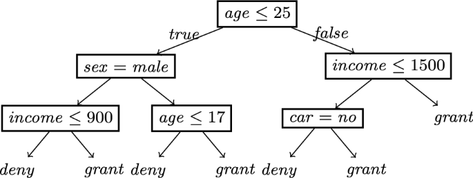
Example of decision tree locally mimicking the black-box behavior

Let assume that the decision tree in Fig. 4 is the merged decision tree c. Let $x \text {=} \{ age \text {=}22$, $sex \text {=} male ,$ $income \text {=}800$, $car \text {=} no \}$ be the instance for which the decision $deny$ (e.g., of a loan) has to be explained. The path followed by x is the leftmost in the tree. The decision rule extracted from the path is $\{ age {\le } 25, sex \text {=} male , income {\le } 900 \} {\rightarrow } deny$. There are four paths leading to $grant$: $q_1\text {=}\{ age {\le } 25, sex \text {=} male , income {>} 900 \}$, $q_2\text {=}\{ 17 {<} age {\le } 25, sex {}\text {=} female \}$, $q_3 \text {=} \{ age {>} 25, income {\le } 1500, car \text {=} yes \}$, and $q_4$ $\text {=}\{ age {>} 25, income {>} 1500\}$. The number of changes for the $q_i$’s are as follow: $nf (q_1, x)\text {=}1$, $nf (q_2, x)\text {=}1$, $nf (q_3, x)$ $\text {=}2$, $nf (q_4, x)\text {=}2$. Therefore, the set of minimal counterfactuals is $\varPhi \text {=} \{ q_1 {\rightarrow } grant ,$ $q_2 {\rightarrow } grant \}$. Assuming that $U \text {=} \{ sex \text {=} male \}$, then $q_2 {\rightarrow } grant$ is not actionable, hence the set of actionable counterfactuals is $\varPhi \text {=} \{ q_1 {\rightarrow } grant \}$.

Finally, we point out that an actionable counterfactual rule $q \rightarrow y'$ can be used to generate an actionable counterfactual instance. Among all possible instances that satisfy $q \rightarrow y'$, we choose the one that differ minimally from x. This is done by looking at the split conditions falsified by x: $\{ sc \in q \ |\ \lnot sc (x) \}$, and selecting for features appearing in an $sc$ the lower/upper bound that is closer to the value of the feature in x. For instance, the $q_1 {\rightarrow } grant$ counterfactual instance of x is $x' = \{ age {=}22, sex {=} male , income {=}900 {+} \epsilon )\}$. We also check that $x'$ constructed in this way is a valid counterfactual, i.e., $b(x') {=} grant$. If this does not occur, $x'$ is not returned as a counterfactual instance.

4.5 Generality: explanations for images, texts and multi-label data

Following the approach of lime (Ribeiro et al. 2016), lore $_{sa}$ can be adapted to work on images and texts. Moreover, inspired by Panigutti et al. (2020), we show how it deals with multi-label data.

Image and Text Data In the pre-processing strategy of lime, an instance in the form of an image or a text is mapped to a vector of binary values. For images, each element in the vector indicates the presence/absence of a contiguous patch of similar pixels (called super-pixels). For words, it indicates the presence/absence of a specific word in the text. This reduces the problem to the analysis of tabular data, and we can reuse lore $_{sa}$ as introduced so far. Due to the binary nature of data involved, the genetic neighborhood approach boils down to generate instances by suppressing super-pixels or words from the instance to explain. This is close to the way that lime works, but with a fitness optimizing approach instead of a purely random suppression. As for lime, the generated instances may not be realistic images or texts.

Multi-labelled Data The formulation of lore $_{sa}$ admits so far binary and multi-class black-boxes. Multi-labelled classifiers return, for an input instance x, one or more class labels. This case is common, for instance, in health data, where more than one disease may be associated with a same list of symptoms. In particular, probabilistic multi-labelled classifiers return a vector of probabilities $b_p(x)$ whose sum is not necessarily 1, as in the multi-class case. Rather, the ith element in $b_p(x)$ is the probability that the ith label is included in the output (with a typical cut-off at 0.5). lore $_{sa}$ can be extended to (probabilistic) multi-labelled black-boxes by adopting multi-class decision trees in the function $buildDecisionTree ()$ of Algorithm 1. Factual rules will be of the form $p \rightarrow y_1, \ldots , y_k$, with $k \ge 1$. Counterfactual rules will be of the form $p[\delta ] \rightarrow y'_1, \ldots , y'_{k'}$, with $k \ge 1$ and such that $\{y_1, \ldots , y_k\} \ne \{y'_1, \ldots , y'_{k'}\}$ (but possibly with proper inclusion).

5 Experiments

After presenting the experimental setting and the evaluation metrics, we compare lore $_{sa}$ against the competitors through: (i) a qualitative comparison of explanations provided, (ii) a quantitative validation of the explanations based on synthetically generated ground truth, and (iii) a quantitative assessment of the proposed method and comparison with state-of-the-art approaches in terms of several metrics.¹⁵ Moreover, the Appendices report further experiments: (iv) comparing different neighborhood generation methods, (v) showing the impact of different distance functions in genetic neighbor generation, (vii) illustrating the effect of the parameters on the genetic neighbor generation, (vii) providing statistical evidence of the differences among lore $_{sa}$ and its competitors, and (viii) reporting on running times.

Table 1 Top: datasets summaries

Table 2 Average accuracy and stddev of the black-box classifiers

5.1 Experimental setup

We experimented with ten tabular datasets, one image dataset, one text dataset, and one multi-labelled dataset. Table 1 reports the dataset details. Almost all tabular datasets have both categorical¹⁶ and continuous features. For most of the datasets, instances regard attributes of an individual person, and the decisions taken by a black-box target socially sensitive tasks.

A random subset of each dataset, denoted by $X_{bb}$, was used to train the black-box classifiers while the remaining part, denoted by X, was used as instances to explain—in brief, the explanation set. For tabular data, the split was 70%-30% and stratified w.r.t. the class attribute. For mnist, 20news, and medical we followed the split custom in the relevant literature.¹⁷ We denote with $\hat{Y} = b(X)$ the decisions of b on X, and with $Y = c(X)$ the decisions of c on X. We assume that the dataset used to train the black-box is unknown at the time of explanation. Hence, we can only rely on the set X of instances to explain. Indeed, the knowledge base K is derived from the explanation set as stated in Footnote 9. Similarly, information about features’ domains required by the competitor methods is computed from X.

We trained and explained the following black-box models: Random Forest (RF), Support Vector Machine (SVM) and Neural Network (NN) as implemented by scikit-learn, and Deep Neural Networks (DNN) implemented by keras.¹⁸ For each black-box, for each dataset, we performed a random search for the best parameter setting.¹⁹ Average classification accuracies are shown in Table 1 (bottom) and in Table 2. We compare lore $_{sa}$ against lime (Ribeiro et al. 2016), maple (Plumb et al. 2018), shap (Lundberg and Lee 2017), anchor (Ribeiro et al. 2018) and brl (Ming et al. 2019). We also compare the counterfactuals of lore $_{sa}$ with the stochastic optimized counterfactuals soc (Russell 2019) as implemented by the alibi library,²⁰ and against the brute force coutnerfactual explainer (bf) as implemented by the fat-forensics library.²¹ Unless stated otherwise, default parameters are used for lore $_{sa}$ and all the other methods.²²

5.2 Evaluation metrics

We evaluate the performances of explanation methods under various perspectives. The measures reported in the following are stated for a single instance to be explained. The metrics obtained as the mean value of the measures over all the instances in the explanation set X, can then be used to evaluate the performances of the explanation methods. Let $x \in X$ be an instance to explain.

Correctness We will evaluate the correctness of explanations under controlled situations where ground truth is available. Let e and $\widetilde{e}$ be the binary vectors indicating the presence/absence (1/0) of a feature in the explanation for x of a given method, and in the ground truth respectively. For rule-based explanations, presence means that the feature appears in the premise of the rule. For feature importance vectors, presence means that the feature has non-zero magnitude. We measure the correctness of an explanation w.r.t. the ground-truth using the f1-score:

$$\begin{aligned} \textit{f1-score}(e,\widetilde{e}) = 2 \cdot \frac{ recall (e,\widetilde{e})\cdot precision (e,\widetilde{e})}{ recall (e,\widetilde{e}) + precision (e,\widetilde{e})} \end{aligned}$$

where the precision is the percentage of features present in e that are also in $\widetilde{e}$, and the recall is the percentage of features in $\widetilde{e}$ that are also in e.

When ground truth is not available, we will consider the following measures to evaluate specific properties of an explanation process.

Silhouette We measure the quality the neighborhood²³ in a local approach by measuring how similar is x to instances in $Z_=$ compared to instances in $Z_{\ne }$. Let d(x, S) denote the mean Euclidean distance between x and instances in S. Inspired by clustering validation (Tan et al. 2005), we define:

$$\begin{aligned} silhouette (x) = \frac{d(x, Z_{\ne })-d(x, Z_{=})}{ max \{d(x, Z_{\ne }), d(x, Z_{=})\}} \end{aligned}$$

High silhouette results from accurate neighborhood generation (Sect. 4.1).

Fidelity It answers the question: how good is the interpretable predictor c at mimicking the black-box b? Fidelity can be measured in terms of accuracy (Doshi-Velez and Kim 2017) of the predictions $Y = c(Z)$ of the interpretable predictor c w.r.t. the predictions $\hat{Y} = b(Z)$ of the black-box b, where Z is the neighborhood of x generated by the local method. High fidelity of c results from both accurate neighborhood generation (Sect. 4.1) and predictive performance of the learning algorithm (Sect. 4.2).

Complexity It is a proxy of the comprehensibility of an explanation, with larger values of complexity denoting harder to understand explanations (Freitas 2013). For rule-based explanations, as complexity we adopt the size of the rule premise (for lore $_{sa}$ we consider only the factual rule). Low complexity results from general (non-overfitting, stable) local interpretable surrogate predictors (Sect. 4.2) and a direct method to extract the rule (Sect. 4.3). For feature importance vectors, as complexity we adopt the number of non-zero features. For instance in lime are those of the local surrogate linear regressor.

Stability It measures the ability to provide similar explanations to similar instances. Also named robustness or coherence, it is a crucial requirement for gaining trust by the users (Guidotti and Ruggieri 2019). We measure it through the local Lipschitz condition (Alvarez-Melis and Jaakkola 2018):

$$\begin{aligned} instability (x) = max _{x_i \in \mathcal {N}_k(x)} \frac{\Vert e_i - e \Vert _2 }{\Vert x_i - x \Vert _2} \end{aligned}$$

(1)

where $\mathcal {N}_k(x)$ is the set of the $k=5$ instances in $X\setminus \{x\}$ closest to x w.r.t. Euclidean distance, e is the binary vector of the explanation of x, and $e_i$ is the binary vector of the explanation of $x_i \in \mathcal {N}_k(x)$. Intuitively, the larger is the ratio the more different are the explanations for instances close to x. Low instability (or, high stability) results from general (non-overfitting, stable) local interpretable surrogate predictors (Sect. 4.2). While low instability could be the result of under-fitting, this is not the case of local explanation methods which, being local and being based on random components, are not prone to exhibit the same explanation for different instances. In addition, we consider also sensitivity of a local explanation method to randomness introduced in the neighborhood generation. This is measured by the distance of explanations generated for a same instance over multiple calls to the explanation method:

$$\begin{aligned} instability _{si}(x) = max _{e_i, e_j \in \mathcal {E}_k(x)} \Vert e_i - e_j \Vert _2 \end{aligned}$$

(2)

where $\mathcal {E}_k(x)$ is the set of the explanations obtained by calling the method $k=5$ times on the same input instance x. A low same-instance instability is obtained when similar explanations are returned over multiple runs. Instances and explanations are normalized before calculating the instability measure.

Coverage and Precision These measures apply to rule-based explanations $p \rightarrow y$ only (for lore $_{sa}$ we consider only the factual rule). Let Z be the neighborhood of x generated by the local method. The coverage of the explanation is the proportion of instances in Z that satisfy p. The precision is the proportion of instances $z \in Z$ satisfying p such that $b(z)=y$. Coverage and precision are competing metrics which respectively estimate the generality of the rule and the probability it correctly models the black-box behavior locally to the instance to explain. They depend both on the characteristics of the neighborhood generation (Sect. 4.1) and on the predictive performance of the learning algorithm (Sect. 4.2).

Changes An indicator of the quality of a counterfactual is the number of changes w.r.t. the instance x. For a set of counterfactual instances, such as those provided by soc, we count the mean number of features whose value is different from x. For a set of counterfactual rules $p[\delta ] \rightarrow y$, provided by lore $_{sa}$, we count the mean number of falsified split conditions $nf (p[\delta ], x)$. For lore $_{sa}$, we expect a small number of changes thanks to the selection of counterfactual paths in the surrogate predictor with minimum number of changes (Sect. 4.3). However, actionability of counterfactuals maybe achieved at the cost of a larger number of changes (Sect. 4.4).

Dissimilarity We measures the proximity between x and the counterfactual $x'$ generated as the distance between x and the counterfactual instance $x'$ that we obtain by applying to x the changes described by $p[\delta ]$. We calculate the distance using the same function described in Sect. 4.1. The lower the better.

Plausibility We evaluate the plausibility of the explanations in terms of the goodness of the counterfactuals returned by using the following metrics based on distance and outlierness Guidotti and Monreale (2020).

Minimum Distance Metric As a straightforward but effective evaluation measure, we adopt proximity. Given the counterfactual $x'$ returned for instance x, $x'$ is plausible if it is not too much different from the most similar instance in a given reference dataset X. Hence, for a given explained instance x, we calculate the plausibility in terms of Minimum Distance $MDM = \min _{\bar{x} \in X / \{x\}}d(x', \bar{x})$ where the lower the MDM, the more plausible is $x'$ the more reliable is the explanation, because $x'$ resembles a real instance in X.

Outlier Detection Metrics We also evaluate the plausibility of the counterfactuals by judging how much they appears as outliers. The lower the scores the more plausible they are. In particular, we estimate the degree of outlierness of a counterfactual $x'$ returned for an instance x by employing the outlier detection technique Isolation Forest (IsoFor) Liu et al. (2008).

5.3 Qualitative evaluation

We qualitatively compare lore $_{sa}$ explanations with those returned by competitors on an instance x of the compas-m dataset, assuming a NN as the black-box. The instance and the explanations are shown in Fig. 5.

The factual rule r of lore $_{sa}$ clarifies that x is considered at high risk of recidivism because of his young age and of the number of previous detections. The counterfactuals $\varPhi$ show that the risk would have been lowered to Low for an older individual, or Medium for various reasons some of which are not actionable, e.g., different age, sex or race. The counterfactuals $\varPhi ^*$ are obtained by considering the set of constraints $U {=} \{$ age=20, age_cat=Less than 25, race=Afr.-Am., sex=Male$\}$. In this case, the decision b(x) would have been different only with a lower number of prior arrests or with a larger number of days between the screening and the arrest.

Fig. 5

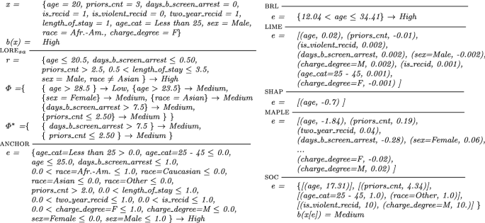
Explanations for an instance x of the compas-m dataset classified as High risk of recidivism by a NN black-box

The competitor rule-based explainers suffer from a few weaknesses. anchor returns various conditions, involving many features, in order to guarantee high precision. Thus, its explanation result hard to read and unnecessarily complex. brl bases its explanation on a rule with a single feature, which on the example instance is age. Even though it is (partly) correct, the user can hardly trust such a simple and minimal justification. We will show next that brl is indeed not particularly good in mimicking black-boxes’ behaviors. The feature importance-based explainers lime, shap and maple provide a list of features with a score of their relevance in the decision. The most important features for lime, i.e., age and priors_cnt, are in line with the factual rule of lore $_{sa}$. shap attributes the decision of the black-box only to age. maple provides a (unnecessarily long) list of features (shortened for space reasons) with scores in agreement with the other explainers. Regarding counterfactuals, soc suggests a set of changes to x’s feature values turning the risk prediction to Medium. Compared to $\varPhi ^*$, the changes are either non-actionable (e.g., age${=}17.31$) or less informative or impossible (e.g., priors_cnt${=}4.34$).

Explanations on Images, Texts & Multi-label Data We compare lore $_{sa}$ explanations for images and texts with lime explanations.

Fig. 6

Explanations of lore $_{sa}$ and lime for two instances x (one per row) of the mnist dataset classified as 9 and 4 by a RF black-box. Meaning of columns is 1st: instance x, 2nd: superpixel segmentation, 3rd: lore $_{sa}$ factual rule, 4–5th: lore $_{sa}$ counterfactuals, $6^{th}$: lime explanation, 7th: lime counterfactuals (towars unspecified class)

Fig. 7

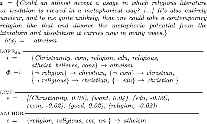
Explanations of lore $_{sa}$ and lime for an instance x of the 20news dataset classified as atheism by a NN black-box

Fig. 8

lore $_{sa}$ explanations for an instance x of the medical dataset classified as Class 12 and Class 38 by a RF black-box

Figure 6 shows such comparison on two images of Fig. mnist. Both methods adopt the same segmentation shown in the second column of the figure. The factual explanations of lore $_{sa}$, shown visually in the 3rd column of Fig. 6, clearly attribute the classifications for 9 and 4 to the presence of super-pixels $s_8$, $s_6$, $s_4$ and $s_7$, $s_0$, $s_4$, respectively. The absence of some of such super-pixels (4th column), would have changed the black-box decision as shown in $\varPhi _1$ and $\varPhi _2$. For instance, the image of 9 would have been classified as 4 if the area of the super-pixel $s_6$ would have been white. The explanation returned by lime are less intuitive both when considering only the super-pixels pushing the classification towards a class (5th column), or pushing the classification towards another (unspecified) class (6th column).

Figure 7 reports the explanations of lore $_{sa}$, lime and anchor for a text from the 20news dataset. All methods adopt the same document vectorization. lore $_{sa}$ shows that the text is classified as atheism because of the simultaneous presence of some words in the factual rule. The absence of specific words in the counterfactual rules would change the classification to christian. lime explanation is in agreement with the one of lore $_{sa}$ as the words edu, com and religion have negative weight on the classification towards atheism. The explanation of anchor highlights the presence of religion and religious, but it also includes less meaningful words.

Figure 8 reports an example of explanation derived for multi-labelled classification using the medical dataset. The instance x is labelled with the diseases corresponding to Class 12 and Class 38. The explanation is the conjunction of symptoms in the factual rule r. A single label would have been returned by the black-box if cough were absent and, either pneumonia were absent or hypertrophy were present. We cannot compare with soc, because it is not able to deal with multi-labelled classification.

In conclusion, we believe that the reported examples of factual, counterfactual, and actionable explanations of lore $_{sa}$ offer to the user a clearer and more trustable understanding than what is offered by the other explainers.

Fig. 9

Correctness metric by varying the total number of features $m+u$. Left: synthetic rule-based classifiers. Right: synthetic linear regressors

5.4 Ground truth validation

By synthetically generating transparent classifiers and using them as black-boxes, we can compare the explanations provided by an explainer with the ground-truth decision logic of the black-box (Guidotti 2021). In particular, the $\textit{f1-score}()$ metric accounts for the correctness of the explanations.

In order to have a comparison as fair as possible among methods returning different types of explanations, we build two types of black-boxes: rule-based classifiers and linear regressor-based. The former are closer to rule-based explainers, the latter to feature importance explainers. In both cases, we start from datasets of m binary informative features and u Gaussian-noise uninformative features. The total number of features $m+u$ varies over $\{2,4,8,16,32,64,128\}$ and, for a fixed $m+u$, we generate 100+100 such datasets where $m<\min \{32, m+u\}$.²⁴ The informative features are generated following the approach of Guyon (2003) implemented in scikit-learn.²⁵ Thus, we have 700 synthetic datasets for training rule-based classifiers and 700 for training linear regressors. Each dataset contains 10,000 instances, 1000 of which are used as explanation set.

Rule-based black-boxes are obtained by training a decision tree from a synthetic dataset, and then extracting rules from such a decision tree. The ground-truth explanation for an instance x is the rule satisfied by x in the black-box. Linear regressors black-boxes are obtained by an adaption of the approach of Klimke (2003). The ground-truth explanation for an instance x is the gradient of the instance in the decision boundary closest to x. Additional details²⁶ can be found in Guidotti (2021).

Figure 9 reports the $\textit{f1-score}$ metric at the variation of the total number of features $m+u$ in synthetic datasets. Each point shows the mean $\textit{f1-score}$ over the explanation sets of such datasets. lore $_{sa}$ outperforms the other explainers when $m + u \le 16$. For larger values of $m + u$, lore $_{sa}$ performance is comparable to those of lime and shap for rule-based classifiers, and slightly lower than their performance for linear regressors.

Table 3 Aggregated evaluation metrics over experimental datasets and black-boxes

5.5 Quantitative evaluation

We quantitatively assess the quality of lore $_{sa}$ and of the competitor explainers through the other evaluation metrics of Sect. 5.2.

In order to evaluate the importance of the trees merging strategy employed by lore $_{sa}$ for deriving the single local decision tree, we implemented a variant that avoids the merging operation. We call it lore $_{sa}^d$ and works as follows. After learning the decision trees $d^{(1)}, d^{(2)}, \ldots , d^{(N)}$ on their corresponding local neighborhood $Z^{(1)}, Z^{(2)}, \ldots , Z^{(N)}$ labeled by the back-box b, we use each tree $d^{(i)}$ for labeling its training neighborhoods, $Z^{(i)}$, i.e., $Y^{(i)}_d = d^{(i)}(Z^{(i)})$. Then, we compute the union of the new labeled neighbors, i.e., $D^Z = \bigcup _{\forall i \in [1,N]}{(Z^{(i)}, Y^{(i)}_d) }$ and we use $D^Z$ to learn the final decision tree c.

For sake of compactness, to quantitatively compare all the explanation methods we report only aggregate results, i.e., mean and standard deviation of the metrics over all datasets and black-boxes. Table 3 (top) reports the silhouette, fidelity, complexity, instability, and instability$_{si}$ metrics. lore $_{sa}$ overcomes all the other explainers on 3 metrics, and it is runner-up on the other 2 metrics. As expected, lore $_{sa}$ considerably improves the complexity and the two instability metrics with respect to its predecessor lore while maintaining the same level of fidelity. In terms of complexity, lore $_{sa}$ is the second best performer after the brl approach which, on the other hand, has lower performance on the other metrics and is one of the most stable. The only competitors with lower instability are shap and maple which provide more complex explanations. Moreover, our experimental results show that lore $_{sa}$ has also lower complexity and instability with respect to lore $_{sa}^d$ highlighting the importance of the merging procedure for the stability. The better performance of lore $_{sa}$ is paid with a slightly higher runtime required to get an explanation due to the merging procedure that is on average 315.59 ± 185.74 seconds among all datasets and black-box models 315.59, while it is on average 285.23 ± 179.83 seconds for lore $_{sa}^d$. We underline that having an efficient implementation is out form the purpose of this paper and that, how specified in the “Appendix”, several possibilities are available to speed up the calculus through parallelization of the explanation process. Figure 10 shows how instability behaves varying the number N of local neighborhoods/decision trees generated by lore $_{sa}$. Similar results are obtained for lore $_{sa}^d$. There is a (local) minimum at $N=5$, which is the value set by default in lore $_{sa}$. Finally, with respect to the instability$_{si}$ metric,²⁷ we point out that brl and maple are deterministic methods, hence the metric does not apply to them. shap, which has the best performances, bases its explanation process on permutations of x with respect to a set of base values. Using a single background value as the medoid of the training set, as suggested in SHAP tutorials’ can markedly limit the variability of the permutations of x. This explains the low instability$_{si}$ value. On the other hand, different background values could lead to different explanations (Gosiewska and Biecek 2020; Sundararajan and Najmi 2020).

Fig. 10

Instability metric by varying the number N of decision trees in lore $_{sa}$

In Table 3 (bottom) we report the coverage and precision metrics for the rule-based explainers under analysis. Furthermore, to capture both measures with a single value, we also report the harmonic mean (h-mean) of coverage and precision. We notice that, lore $_{sa}$, lore $_{sa}^d$ and lore overcome anchor and brl for both indicators. lore $_{sa}$ considerably improves the rule coverage paying something in precision; however, looking at the h-mean lore $_{sa}$ is the best performer. This is another beneficial effect of the bagging-like approach, which improves on generality (less overfitting) of the interpretable predictor. A Friedman test (Demsar 2006) on each of the metrics rejects the null hypothesis of zero difference among the methods (p value $< 10^{-5}$). Further evidence is reported in “Appendix D”.

Table 4 Aggregated evaluation metrics estimating the proximity of the counterfactual explanations in terms of dissimilarity and the plausibility as MDM and IF scores

Table 4 compares lore $_{sa}$ with the merging variant and with two competitors with respect to the counterfactual part of the explanation. We highlight that lore $_{sa}$ is not an explainer directly returning counterfactual instances on its own. However, counterfactual instances can be created by modifying the instance under analysis x according to the counterfactual rules in $\varPhi$. We notice that the brute force approach bf has the lowest dissimilarity but lore $_{sa}$ and lore $_{sa}^d$ achieve closer results. soc is the worst performer with respect to this metric, meaning that the counterfactual instances returned by soc are not highlighting minimal changes with respect to x to change decision. Furthermore, lore $_{sa}$ alternatives return the most plausible counterfactuals with respect to the the MDM and IsoFor metrics. There is not a clear winner but overall the plausibility scores of lore $_{sa}$ are better being always the best performer or the runner up, i.e., lower, than those of bf and soc, enabling it to be used also as a possible counterfactual explainer.

Table 5 Aggregated evaluation metrics for counterfactuals over experimental datasets and black-boxes

In Table 5, we compare lore $_{sa}$ with the counterfactual explainer soc that is typically used as a baseline (Guidotti 2022). Mean and standard deviations are reported for the number of counterfactual instances (soc) or counterfactual rules (lore $_{sa}$) produced, and the changes metrics (number of changes to instance x to revert the black-box outcome). For all the reported datasets and black-boxes, lore $_{sa}$ produce less changes than soc. On the other hand, soc returns more counterfactuals. The number of counterfactuals returned by lore $_{sa}$ could be increased trading off with changes, simply by relaxing the requirement of minimality in Algorithm 3. Let us now denote with lore $_{s\underline{a}}$ with underlined a the execution of lore $_{sa}$ with in input dataset-specific constraints U stating features that cannot be changed: $age$, $race$, $sex$, $native\text {-}country$, $marital\text {-}status$ for adult; $age$ for bank; $state$, $state\text {-}area$, $state$ for churn; $age ,$ $age\text {-}cat$, $race$, $sex$ for compas-m (shown as cps-m in the table). As expected, it turns out that lore $_{s\underline{a}}$ produces less counterfactuals its counterpart ignoring the actionability. This is due to the filtering of the counterfactual rules that do not satisfy the feature constraints. On average, such counterfactual require more changes to the instance x to explain, but still less than soc.

6 Conclusion

We have proposed lore $_{sa}$, a black-box agnostic method for local explanations providing informative factual decision rules and actionable counterfactual rules. An ample experimental evaluation with state-of-the-art methods has shown that lore $_{sa}$ largely improves as per stability of explanations, while ranking top or runner-up in several other quantitative metrics. Stability of the provided explanations is achieved by adopting a novel bagging-like approach in generating and aggregating several local decision trees.

A few directions can be mentioned as future work to expand the applicability of lore $_{sa}$. First, synthetically generated instances may not respect correlations among attributes (e.g., age and education level). Hence, it is worth extending the approach by integrating domain knowledge (dependencies or causal relationships) among attributes in the neighborhood generation and/or in the inference of the interpretable predictor. Second, in multi-class problems, alternative definitions of $fitness _{\ne }$ could be implemented to drive the selection of counterfactual rules towards some specific class value. E.g., in a credit risk rating context, to provide counterfactuals toward a lower risk label. Third, the adaptation of lore $_{sa}$ to images and texts with a simple binary encoding, modeling presence/absence of a super-pixel/word, suffers from the same problems as lime, namely the generation of unrealistic synthetic instances. More complex encoding using autoencoders can be used to overcome these limitations and to produce neighborhoods of realistic images and texts (Guidotti et al. 2019c). Finally, lore $_{sa}$ assumes that the black-box can be queried as many times as necessary. When this is not the case, the neighborhood generation phase must take into account constraints on the number of admissible queries, e.g., by adopting an active learning variant of the genetic approach.

Appendices

Neighborhood generation

Table 6 Aggregated evaluation metrics over datasets (top) and black-boxes (bottom)

In Sect. 5, we contrasted lore $_{sa}$ with lore, which adopts a simplified fitness function where the distance between class probability vectors (namely, $l(b_p(x),b_p(z))$ in $fitness ^x_{=}(z)$) is replaced by identity of the predictions (namely, $I_{b(x)=b(z)}$), and which consider a single neighborhood/decision tree. Here, we conduct an ablation study by contrasting lore $_{sa}$ with a version of it including a purely random neighborhood generation, called rnd$_{sa}$. Table 6 reports the evaluation metrics described in Sect. 5.2 for the experimental datasets and black-box classifiers. The best results are highlighted in bold. lore $_{sa}$ has nearly always the best silhouette, fidelity, precision, and instability. The best performing silhouette of lore $_{sa}$ confirms that the genetic neighborhood generation strategy leads to dense neighborhoods with instances that separate the local decision boundary and they are still similar to the one to explain. Hence, it is not just a marginal improvement over random generation but a key feature to achieve compactness and separation of the neighborhoods $Z_{=}$ and $Z_{\ne }$. Other basic techniques of neighborhood generation, such as oversampling and instance selection, are also overcome by the genetic approach, as shown in Guidotti et al. (2019b). For black-box aggregations, rnd$_{sa}$ shows the best coverage and complexity. This can be attributed to a weaker, hence simpler, decision boundary characterization of the purely random strategy.

Impact of distance functions

Table 7 Aggregated evaluation metrics over datasets (top) and black-boxes (bottom) w.r.t. distance functions in the neighborhood generation of lore $_{sa}$

A key element of the neighborhood generation is the distance function used by the genetic algorithm. In this section we show how the explanations of lore $_{sa}$ are affected by different distance functions. For example, Wachter (2017) shows that considerable differences of the counterfactual instances occur at the variation of the distance function adopted by their stochastic optimization approach. As alternative distances to the normalized euclidean distance (neucliden) adopted by lore $_{sa}$, we report results using the cosine distance and the normalized mean deviation (nmeandev) distance. Experiments over the compas, fico and german datasets, and over DNN, NN, and SVM black-boxes are reported in Table 7. There is no major difference in terms of fidelity and precision, whilst neucliden has the best performance or is a close runner up for all other metrics.

Genetic algorithm parameters

Fig. 11

Mean values of fitness functions at the last generation of Algorithm 2 on the compas dataset and DNN black-box by varying parameters

Fig. 12

Aggregated evaluation metrics on the compas dataset and DNN black-box by varying the parameters of Algorithm 2. Scale on the right y axis is for complexity

We investigate on the impact of the parameters of the genetic Algorithm 2: (i) the neighborhood size n, (ii) the crossover probability $p_c$, (iii) the mutation probability $p_m$, and (iv) the number of generations g. We vary one parameter at a time while keeping the others fixed at their default value, i.e., $n=500$, $p_c = 0.7$, $p_m = 0.5$, $g=20$, $N=5$ (recall that $n=500$ implies that the neighborhood $Z^{(i)} = Z^{(i)}_= \cup Z^{(i)}_{\ne }$ consists of $2n = 1000$ instances). Experiments are performed on the compas dataset and using the RF as black-box. Figure 11 shows the average values of the two fitness functions at the last generation for the two components of the neighborhood: $Z_=$ and $Z_{\ne }$. Regarding n, values greater than 1000 do not lead to a net increase of the fitness functions. A similar behavior is observed for $g \approx 20$–50. On the other hand, varying crossover and mutation probabilities does not make appreciable impact on the fitness functions. To better understand their impact, we analyze in Fig. 12 some evaluation metrics while varying the parameters as before²⁸. With respect to the neighborhood size n, for $n>1000$, complexity grows remarkably, whist all other metrics become stable. Similarly,the crossover probability $p_c$ does not affect any metric but the complexity. The mutation probability $p_m$ appears negatively correlated to coverage, silhouette, and complexity. Finally, a very low number of generations g lead to bad results, while for $g > 10$, all the metrics become stable. In summary, the default values for the parameters $n = 1000$, $g = 20$, and $p_m = 0.5$ were chosen experimentally based on the previous discussion. Regarding the cross-over parameter $p_c = 0.7$, we departed from a 50–50 choice in favor of the diversity of generated instances.

Table 8 Mean rank of explainers by dataset over all combinations of black-boxes and metrics (silhouette, fidelity, complexity, instability)

Table 9 Mean rank over all combinations of datasets and evaluation metrics

Fig. 13

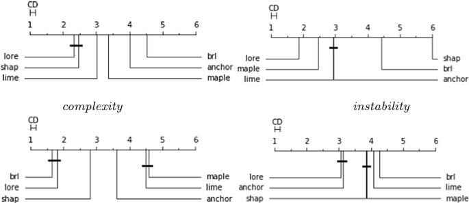
Critical difference diagrams using the Nemenyi test at $\alpha =0.05$. The name lore in the plots indicate the lore $_{sa}$ method

Table 10 Running time (mean ± stdev) in secs for SVM

Statistical tests

Tables 8 and 9 report the mean rank values (ranging from 1 to 6) among the different explainers for a given dataset (resp., black-box) over all combinations of black-boxes (resp., datasets), and of the evaluation metrics of silhouette, fidelity, complexity, and instability. The first column of Table 8 reports the overall mean rank. It is readily checked that lore $_{sa}$ ranks the best in general (p value $< 0.001$ using a Wilcoxon signed rank test), for each dataset, and for each black-box. For the compas-m, bank and fico datasets and for the RF and SVM black-boxes, lore $_{sa}$ ranks markedly higher than the competitors. Figure 13 shows four Critical Difference (CD) diagrams (Demsar 2006). They display the statistical significance of the observed paired differences in performances between pairs of the explanation methods. Two methods are tied if the null hypothesis that their performances are the same cannot be rejected using the Nemenyi test at $\alpha {=}0.05$. lore $_{sa}$ performs better than the compared methods with regards to fidelity, and the differences are statistically significant. For each of the other metrics, the method tied to lore $_{sa}$ is always a different one. Hence, lore $_{sa}$ wins over any other method in at least 3 out of the 4 metrics.

Running time

Table 10 reports the running time (in secs) of producing an explanation for three experimental datasets and for the SVM black-box. lore $_{sa}$ performances are in line with anchor and soc, and better than maple and brl. They are instead worse than lime and shap. The vast majority of running time ($>90$%) of lore $_{sa}$ is used by the genetic neighborhood generation. The implementation, however, can be readily sped up by parallelising the generation of $Z_{=}^{(1)}, Z_{\ne }^{(1)}, \ldots , Z_{=}^{(N)}, Z_{\ne }^{(N)}$ ($2\cdot N$ independent calls to Algorithm 2).

References

Adadi A, Berrada M (2018) Peeking inside the black-box: a survey on explainable artificial intelligence (XAI). IEEE Access 6:52138–52160
Alvarez-Melis D, Jaakkola TS (2018) Towards robust interpretability with self-explaining neural networks. In: NeurIPS, pp 7786–7795
Angelino E, Larus-Stone N, Alabi D, Seltzer MI, Rudin C (2017) Learning certifiably optimal rule lists for categorical data. J Mach Learn Res 18:234:1-234:78
Assche AV, Blockeel H (2007) Seeing the forest through the trees: learning a comprehensible model from an ensemble. In: ECML. Lecture notes in computer science, vol 4701. Springer, pp 418–429
Bäck T, Fogel DB, Michalewicz Z (2000) Evolutionary computation 1: basic algorithms and operators, vol 1. CRC Press, Boca Raton
Bénard C, Biau G, Veiga SD, Scornet E (2019) SIRUS: making random forests interpretable. CoRR arXiv:1908.06852
Berk R, Heidari H, Jabbari S, Kearns M, Roth A (2018) Fairness in criminal justice risk assessments: the state of the art. Sociol Methods Res 50(1):3–44
Bhatt U, Xiang A, Sharma S, Weller A, Taly A, Jia Y, Ghosh J, Puri R, Moura JMF, Eckersley P (2020) Explainable machine learning in deployment. In: FAT*, ACM, pp 648–657
Breiman L (1996) Bagging predictors. Mach Learn 24(2):123–140
Breiman L (2001) Statistical modeling: the two cultures (with comments and a rejoinder by the author). Stat Sci 16:199–231
Breiman L, Friedman JH, Olshen RA, Stone CJ (1984) Classification and regression trees. Wadsworth, Belmont
Byrne RM (2016) Counterfactual thought. Annu Rev Psychol 67(1):135–157
Byrne RMJ, Johnson-Laird P (2009) “If’’ and the problems of conditional reasoning. Trends Cogn Sci 13(9):282–287
Calegari R, Ciatto G, Denti E, Omicini A (2020) Logic-based technologies for intelligent systems: state of the art and perspectives. Information 11(3):167
Chou Y, Moreira C, Bruza P, Ouyang C, Jorge JA (2022) Counterfactuals and causability in explainable artificial intelligence: theory, algorithms, and applications. Inf Fusion 81:59–83
Darwiche A, Hirth A (2020) On the reasons behind decisions. In: ECAI, IOS Press, frontiers in artificial intelligence and applications, vol 325, pp 712–720
Demsar J (2006) Statistical comparisons of classifiers over multiple data sets. J Mach Learn Res 7:1–30
Derrac J, García S, Herrera F (2010) A survey on evolutionary instance selection and generation. Int J Appl Metaheuristic Comput 1(1):60–92
Doshi-Velez F, Kim B (2017) A roadmap for a rigorous science of interpretability. CoRR arXiv:1702.08608
Evans BP, Xue B, Zhang M (2019) What’s inside the black-box? A genetic programming method for interpreting complex machine learning models. In: GECCO, ACM, pp 1012–1020
Fan C et al (2020) Classification acceleration via merging decision trees. In: FODS, ACM, pp 13–22
Fortin F, Rainville FD, Gardner M, Parizeau M, Gagné C (2012) DEAP: evolutionary algorithms made easy. J Mach Learn Res 13:2171–2175
Freitas AA (2013) Comprehensible classification models: a position paper. SIGKDD Explor 15(1):1–10
Fu Y, Zhu X, Li B (2013) A survey on instance selection for active learning. Knowl Inf Syst 35(2):249–283
Gosiewska A, Biecek P (2020) Do not trust additive explanations. CoRR arXiv:1903.11420
Guidotti R (2021) Evaluating local explanation methods on ground truth. Artif Intell 291:103428
Guidotti R (2022) Counterfactual explanations and how to find them: literature review and benchmarking. Data Min Knowl Discov. https://doi.org/10.1007/s10618-022-00831-6
Guidotti R, Monreale A (2020) Data-agnostic local neighborhood generation. In: ICDM, IEEE, pp 1040–1045
Guidotti R, Ruggieri S (2019) On the stability of interpretable models. In: IJCNN, IEEE, pp 1–8
Guidotti R, Monreale A, Cariaggi L (2019a) Investigating neighborhood generation methods for explanations of obscure image classifiers. In: PAKDD (1). Lecture notes in computer science, vol 11439. Springer, pp 55–68
Guidotti R, Monreale A, Giannotti F, Pedreschi D, Ruggieri S, Turini F (2019b) Factual and counterfactual explanations for black box decision making. IEEE Intell Syst 34(6):14–23
Guidotti R, Monreale A, Matwin S, Pedreschi D (2019c) Black box explanation by learning image exemplars in the latent feature space. In: ECML/PKDD (1). Lecture notes in computer science, vol 11906. Springer, pp 189–205
Guidotti R, Monreale A, Ruggieri S, Turini F, Giannotti F, Pedreschi D (2019d) A survey of methods for explaining black box models. ACM Comput Surv 51(5):93:1-93:42
Guyon I (2003) Design of experiments of the NIPS 2003 variable selection benchmark. In: NIPS workshops
Holland JH (1992) Adaptation in natural and artificial systems: an introductory analysis with applications to biology, control, and artificial intelligence. MIT Press, Cambridge
Jia Y, Bailey J, Ramamohanarao K, Leckie C, Houle ME (2019) Improving the quality of explanations with local embedding perturbations. In: KDD, ACM, pp 875–884
Karimi A, Barthe G, Schölkopf B, Valera I (2020) A survey of algorithmic recourse: definitions, formulations, solutions, and prospects. CoRR arXiv:2010.04050
Klimke A (2003) RANDEXPR: a random symbolic expression generator. Technical report 4, Universitat Stuttgart
Lakkaraju H, Bach SH, Leskovec J (2016) Interpretable decision sets: a joint framework for description and prediction. In: KDD, ACM, pp 1675–1684
Laugel T, Renard X, Lesot M, Marsala C, Detyniecki M (2018) Defining locality for surrogates in post-hoc interpretablity. CoRR arXiv:1806.07498
Li X, Cao CC, Shi Y, Bai W, Gao H, Qiu L, Wang C, Gao Y, Zhang S, Xue X, Chen L (2022) A survey of data-driven and knowledge-aware explainable AI. IEEE Trans Knowl Data Eng 34(1):29–49
Liu FT, Ting KM, Zhou ZH (2008) Isolation forest. In: 2008 eighth IEEE international conference on data mining, IEEE, pp 413–422
Lucic A, Oosterhuis H, Haned H, de Rijke M (2019) Actionable interpretability through optimizable counterfactual explanations for tree ensembles. CoRR arXiv:1911.12199
Lucic A, Haned H, de Rijke M (2020) Why does my model fail? Contrastive local explanations for retail forecasting. In: FAT*, ACM, pp 90–98
Lundberg SM, Lee S (2017) A unified approach to interpreting model predictions. In: NIPS, pp 4765–4774
Malgieri G, Comandé G (2017) Why a right to legibility of automated decision-making exists in the GDPR. Int Data Privacy Law 7(4):243–265
McCane B, Albert M (2008) Distance functions for categorical and mixed variables. Pattern Recognit Lett 29(7):986–993
Miller T (2019) Explanation in artificial intelligence: insights from the social sciences. Artif Intell 267:1–38
Ming Y, Qu H, Bertini E (2019) Rulematrix: visualizing and understanding classifiers with rules. IEEE Trans Vis Comput Graph 25(1):342–352
Minh D, Wang HX, Li YF, Nguyen TN (2022) Explainable artificial intelligence: a comprehensive review. Artif Intell. Review To appear
Molnar C (2019) Interpretable machine learning. Lulu Press, Morrisville
Moraffah R, Karami M, Guo R, Raglin A, Liu H (2020) Causal interpretability for machine learning: problems, methods and evaluation. SIGKDD Explor 22(1):18–33
Mothilal RK, Sharma A, Tan C (2020) Explaining machine learning classifiers through diverse counterfactual explanations. In: FAT*, ACM, pp 607–617
Murthy SK, Kasif S, Salzberg S (1994) A system for induction of oblique decision trees. J Artif Intell Res 2:1–32
Ntoutsi E et al (2020) Bias in data-driven artificial intelligence systems: an introductory survey. WIREs Data Min Knowl Discov 10(3):e1356
Olvera-López JA, Carrasco-Ochoa JA, Trinidad JFM, Kittler J (2010) A review of instance selection methods. Artif Intell Rev 34(2):133–143
Panigutti C, Guidotti R, Monreale A, Pedreschi D (2020) Explaining multi-label black-box classifiers for health applications. In: Precision health and medicine, studies in computational intelligence, vol 843. Springer, pp 97–110
Pasquale F (2015) The black box society: the secret algorithms that control money and information. Harvard University Press, Cambridge
Pedreschi D, Giannotti F, Guidotti R, Monreale A, Ruggieri S, Turini F (2019) Meaningful explanations of black box AI decision systems. In: AAAI, AAAI Press, pp 9780–9784
Plumb G, Molitor D, Talwalkar AS (2018) Model agnostic supervised local explanations. In: NeurIPS, pp 2520–2529
Ribeiro MT, Singh S, Guestrin C (2016) "Why should I trust you?": explaining the predictions of any classifier. In: KDD, ACM, pp 1135–1144
Ribeiro MT, Singh S, Guestrin C (2018) Anchors: high-precision model-agnostic explanations. In: AAAI, AAAI Press, pp 1527–1535
Rudin C (2019) Stop explaining black box machine learning models for high stakes decisions and use interpretable models instead. NMI 1:206
Russell C (2019) Efficient search for diverse coherent explanations. In: FAT, ACM, pp 20–28
Sagi O, Rokach L (2018) Ensemble learning: a survey. WIREs Data Min Knowl Discov 8(4):e1249
Sagi O, Rokach L (2020) Explainable decision forest: transforming a decision forest into an interpretable tree. Inf Fusion 61:124–138
Sharma S, Henderson J, Ghosh J (2019) CERTIFAI: counterfactual explanations for robustness, transparency, interpretability, and fairness of artificial intelligence models. CoRR arXiv:1905.07857
Shih A, Choi A, Darwiche A (2018) A symbolic approach to explaining Bayesian network classifiers. In: IJCAI, ijcai.org, pp 5103–5111
Sokol K, Flach PA (2019) Desiderata for interpretability: explaining decision tree predictions with counterfactuals. In: AAAI, AAAI Press, pp 10035–10036
Strecht P, Mendes-Moreira J, Soares C (2014) Merging decision trees: a case study in predicting student performance. In: ADMA. Lecture notes in computer science, vol 8933. Springer, 535–548
Sundararajan M, Najmi A (2020) The many Shapley values for model explanation. In: ICML, PMLR, proceedings of machine learning research, vol 119, pp 9269–9278
Tan P, Steinbach MS, Kumar V (2005) Introduction to data mining. Addison-Wesley, Reading
Tsai C, Eberle W, Chu C (2013) Genetic algorithms in feature and instance selection. Knowl Based Syst 39:240–247
Venkatasubramanian S, Alfano M (2020) The philosophical basis of algorithmic recourse. In: FAT*, ACM, pp 284–293
Verma S, Dickerson JP, Hines K (2020) Counterfactual explanations for machine learning: a review. CoRR arXiv:2010.10596
Vidal T, Schiffer M (2020) Born-again tree ensembles. In: ICML, PMLR, proceedings of machine learning research, vol 119, pp 9743–9753
Virgolin M, Alderliesten T, Bosman PAN (2020) On explaining machine learning models by evolving crucial and compact features. Swarm Evol Comput 53:100640
Wachter S et al (2017) Counterfactual explanations without opening the black box. Harv JL Technol 31:841
Wu S, Olafsson S (2006) Optimal instance selection for improved decision tree induction. In: IIE, IISE, p 1
Yang H, Rudin C, Seltzer MI (2017) Scalable Bayesian rule lists. In: ICML, PMLR, proceedings of machine learning research, vol 70, pp 3921–3930
Zafar MR, Khan NM (2019) DLIME: a deterministic local interpretable model-agnostic explanations approach for computer-aided diagnosis systems. CoRR arXiv:1906.10263
Zhang Y, Song K, Sun Y, Tan S, Udell M (2019) Why should you trust my explanation? Understanding uncertainty in LIME. arXiv:1904:12991
Funding
Open access funding provided by Università di Pisa within the CRUI-CARE Agreement. This work has been partially supported by the European Community Horizon 2020 programme under the funding schemes: G.A. 871042 SoBigData++ (sobigdata), G.A. 952026 HumanE AI Net (humane-ai), G.A. 834756 XAI (xai), G.A. 871042 NoBIAS (nobias), G.A. 952215 TAILOR (tailor), and CHIST-ERA grant CHIST-ERA-19-XAI-010, by MUR (N. not yet available), FWF (N. I 5205), EPSRC (N. EP/V055712/1), NCN (N. 2020/02/Y/ST6/00064), ETAg (N. SLTAT21096), BNSF (N. KP-06-AOO2/5) SAI (sai).
Author information
Authors and Affiliations
Contributions
RG: Conceptualization, Methodology, Software, Validation, Formal analysis, Investigation, Resources, Data Curation, Writing—Original Draft, Writing—Review and Editing, Visualization. AM: Conceptualization, Methodology, Resources, Writing—Original Draft, Writing—Review and Editing. SR: Conceptualization, Methodology, Resources, Writing—Original Draft, Writing—Review and Editing. FN: Software, Validation, Experiments. FT: Conceptualization, Supervision, Resources, Writing—Review and Editing. DP: Conceptualization, Supervision, Project administration, Funding acquisition. FG: Conceptualization, Supervision, Project administration, Funding acquisition.
Corresponding author
Ethics declarations
Conflict of interest
The authors declare that they have no conflict of interest.
Ethical approval
Not applicable.
Consent to participate
Consent for publication
The authors declare that they all provide consent for publication.
Additional information
Responsible editor: Martin Atzmüller.
Publisher's Note
Springer Nature remains neutral with regard to jurisdictional claims in published maps and institutional affiliations.