Unsupervised anomaly detection in multivariate time series with online evolving spiking neural networks

Abstract

With the increasing demand for digital products, processes and services the research area of automatic detection of signal outliers in streaming data has gained a lot of attention. The range of possible applications for this kind of algorithms is versatile and ranges from the monitoring of digital machinery and predictive maintenance up to applications in analyzing big data healthcare sensor data. In this paper we present a method for detecting anomalies in streaming multivariate times series by using an adapted evolving Spiking Neural Network. As the main components of this work we contribute (1) an alternative rank-order-based learning algorithm which uses the precise times of the incoming spikes for adjusting the synaptic weights, (2) an adapted, realtime-capable and efficient encoding technique for multivariate data based on multi-dimensional Gaussian Receptive Fields and (3) a continuous outlier scoring function for an improved interpretability of the classifications. Spiking neural networks are extremely efficient when it comes to process time dependent information. We demonstrate the effectiveness of our model on a synthetic dataset based on the Numenta Anomaly Benchmark with various anomaly types. We compare our algorithm to other streaming anomaly detecting algorithms and can prove that our algorithm performs better in detecting anomalies while demanding less computational resources for processing high dimensional data.

1 Introduction

Detecting outliers in time series data, especially streaming data, has gained significant relevance due to the recent exponential growth in the amount of data captured in big-data and IoT applications (Ahmad et al. 2017; Munir et al. 2019; Macia̧g et al. 2021). Particularly the detection of anomalies in streaming time series data places high demands on the development of effective and efficient algorithms (Ahmad et al. 2017). Real-time capable algorithms are required for many applications in order to process these generated or recorded data. In many cases it is not easy to collect sufficient training data with marked anomalies for the supervised training of an anomaly detector to identify anomalies in data streams (Macia̧g et al. 2021). It is therefore particularly important to design anomaly detectors that can correctly classify anomalies from data where none of the input values need to be classified. Ideally, the designed anomaly detector should learn in an online mode in which the current input values adjust the parameters of the detector for better anomaly detection of future input data. Since conventional machine learning algorithms are in many cases unable to cope with these requirements or can only handle them with a large expenditure of resources, there is a great interest in new efficient solutions. Spiking neural networks have the capability for processing information in a fast way, both in terms of energy and data, due to their functional similarity to the brain (Bing et al. 2018a; Gerstner and Kistler 2002; Lobo et al. 2018) thus they are particularly well suited for online detection of anomalies. Although they are one of the major exponents of the third generation of artificial neural networks, it took a while till they were applied to an online learning approach (Lobo et al. 2018, 2020).

In this paper, we extend an existing algorithm for anomaly detection by Maciąg et al. (2021) from the field of evolving Spiking Neural Networks, in which learning processes, neural communication and classification of data instances are based exclusively on spike exchange between neurons. The approach by Maciąg et al. (2021) is however solely designed for univariate time series. Since multivariate data streams are in practice quiet common we contribute in this work several appropriate measures to make the algorithm work for multivariate data. Here, we focused both on the runtime and real-time capability of the algorithm as well as the general performance for the detection of different types of anomalies which are presented in appendix A.1. Our results can be summarized in the following way:

• We present an online capable encoding technique for multivariate times series data. Our method is based on the work of Panuku and Sekhar (2008). It provides a significant performance boost to a parallel execution of several univariate versions of the algorithm of Maciąg et al. (2021).

• We use a new continuous outlier score, which is adapted from Ahmad et al. (2017). This outlier score can be executed in an online manner and provides significantly better results as the currently used technique in Maciąg et al. (2021).

• We apply the SpikeTemp learning approach by Wang et al. (2017) as an improvement for the existing technique and therefore getting better and faster results for anomaly detection even in the univariate case.

Compared to deep learning models the main advantage of our model is, that it needs no time for training and less memory space, while its performance is in a similar range (see Geiger et al. 2020 and Sect. 5). In the following we use outlier for anomalous data points as well as anomaly. The difference between an outlier and an anomaly is small (see Aggarwal 2013) and some authors use both expressions as well, i.e. Shukla and Sengupta (2020).

2 Related work

Due to the extensive demand for efficient and versatile algorithms for outlier detection a wide variety of approaches has been studied in the existing literature. Depending on the application domain, different kinds of algorithms and techniques have been used. In the following section we present a general review of currently available related literature sources regarding to either univariate or multivariate unsupervised and semi-supervised outlier detection in time series given the applicability of these techniques in a streaming scenario.

One of the most commonly used technique for detecting outliers in a wide variety of different application domains is the Local Outlier Factor (LOF) as proposed by Breunig et al. (2000). This technique uses a density measure which describes how isolated a given instance is with regards to its neighborhood. Pokrajac et al. (2007) proposed an incremental version of this algorithm that makes it suitable for an efficient detection of outliers in data streams. Both the static as well as the incremental LOF algorithm are not designed for high dimensional data as well as for temporal relationships in the input data (Gühring et al. 2019; Pokrajac et al. 2007), thus making it unapplicable for those specific applications.

Statistical autoregressive (AR) models such as ARIMA, VAR, VARIMA have also been extensively studied in the past for detecting outliers in both univariate and multivariate time series (Hau and Tong 1989; Moayedi and Masnadi-Shirazi 2008; Li et al. 2019b). These kinds of models particularly excel by their simplicity and the lack of an initially required training phase and are therefore also suitable for streaming data processing. However, since ARIMA models can barely handle nonlinear relationships, their approach to complex real-world problems is not always satisfactory (Zhang 2003).

Recent advances in deep learning like natural language processing (NLP) or speech recognition have caused an increasing utilization of various network architectures in outlier detection research (Chalapathy and Chawla 2019). These range from Convolutional Neural Networks (CNN), Long Short Term Memory (LSTM) Networks, Autoencoders up to Generative Adversarial Networks. Both discriminative and generative models are used in this context. However, due to the pronounced class imbalance and the associated lack of appropriate data labels, discriminative models are used far less often. Fu et al. (2019) proposed a CNN based denoising autoencoder architecture for detecting outliers in time series data. The autoencoder structure is used for unsupervised feature learning of variable groups and is complemented by a classification layer that distinguishes normal from abnormal samples. Another time series anomaly detection method based on deep learning was proposed by Mahotra et al. (2016). With their EncDec-AD LSTM architecture they propose an encoder decoder scheme for reconstructing the given input signal using the compressed vector representation of the decoder. In order to compute the likelihood of an anomaly they model a normal distribution over the determined error vectors. Generative Adversarial Networks are also extensively present in current research. Geiger et al. (2020) and Li et al. (2019a) both use an adversarial minimax training approach on an LSTM architecture in order to detect outliers in time series. Both use the discriminative and the reconstructive components of the architecture in order to distinguish fake from real data using a multi component outlier scoring system. Deep learning based architectures, however, require for training and inference a vast amount of computing power, making an application of these approaches in a streaming context especially on low power devices infeasible.

To exploit the advances from both, the traditional approaches for outlier detection and deep neural networks there is currently an increased use of hybrid models that are either used in order to improve the quality, the speed or the scalability of the algorithm. Munir et al. (2019) uses a combination of an ARIMA model and a two layered Convolutional Neural Network in a residual learning scheme for the prediction of a given time series where both models complement each other for optimal results. This information is then further utilized for detecting existing outliers in the signal using the Euclidean distance between the real and predicted time step. Another hybrid model is proposed by Shukla and Sengupta (2020). They use a combination of hierarchical clustering and a Long Short Term Memory Network (LSTM) where the hierarchical clustering condenses similar correlating input data which are then fed into a LSTM network enabling the architecture to scale well for high dimensional data. Papadimitriou et al. (2005) proposed a neural network type architecture (SPRIT) for detecting outliers in data streams by reconstructing a given time series using a dynamic repository of incrementally estimated principal components which are approximated by the weights of a hidden neuron. The number of required eigencomponents is determined by a heuristic, which compares the energy of the input data and the estimated eigencomponents. Since each additional added principal component can summarize further aspects of the signal which cannot be explained by the previous principal components, an increase of the repository indicates the existence of an outlier in the current time step.

Advances in neuroscientific disciplines produced a large number of novel approaches of biological plausible learning algorithms for the detection of anomalies in signals. A heavily biologically inspired learning approach used in current anomaly detection research are Spiking Neural Networks (SNN). Xing et al. (2019) proposed a hybrid learning approach using a combination of an evolving Spiking Neural Network architecture as well as a restricted Boltzmann machine for detecting outliers in time series. The concept of an evolving Spiking Neural Network architecture for the efficient processing of data streams is used in several other publications. Demertzis et al. (2017, 2019) use in multiple papers an evolving Spiking Neural Network approach based on a simplified Leaky Integrate and Fire model (LIF) and a Rank Order Coding scheme in a semi-supervised learning scenario. Maciąg et al. (2021) use a similar architecture for an Online evolving Spiking Neural network to detect signal outliers in time series data in an online mode using the error between the reconstructed and the given time series. The evolving architecture used by the previously mentioned approaches enable a continuous adaption to changing statistics of input data, making them well suited for online learning (Wysoski et al. 2006).

3 Pattern discovery in multivariate time series

In this paper we present an online capable algorithm, which is able to detect anomalies in multivariate time series. The detection of anomalies in multivariate times series is not the same as detecting anomalies in a single valued time series, since also correlations between the different dimensions have to be taken into account. Since this is also one of the main differences between our paper and the work of Macia̧g et al. (2021), we here present as a benchmark algorithm the SPIRIT algorithm, another algorithm focusing on outlier detection of streaming multivariate time series. Streaming Pattern dIscoveRy in multIple Time-series (SPRIT) by Papadimitriou et al. (2005) is a fast online capable multivariate time series algorithm. It is according to Aggarwal (2013) one of the most well known unsupervised algorithms which is designed to work not only on single data streams but takes into account a global direction of correlation between different simultaneous data streams. In order to evaluate multivariate time series for anomaly detection most of the time a method for dimensionality reduction is used. The SPIRIT algorithm uses an online principal component analysis for this task. We explain it here in more detail.

The goal of the SPIRIT algorithm is to approximate a representation of the input signal with the smallest possible number of principal components. The algorithm does not require an initial training phase as the principal components are continuously updated with incoming data points $\mathbf {x}_{t} = \left[ x_{t,1},\ldots ,x_{t,n}\right] ^T$ of the n-dimensional data stream.

The principal components matrix of the form $W \in {\mathbb {R}}^{n \times k}$ where n is the number of dimensions of the incoming signal and k is the number of the current principal components are initially represented by the conical unit vector $\mathbf {u} = \left[ u_{1} \dots u_{k}\right]$. For each time step the eigencomponents making up the matrix W are updated. Therefore the current data point $\mathbf {x}_{t}$ is used to initialize the temporary variable $\acute{\mathbf {x}}_{1}$ which is used to calculate the projection $\mathbf {y}$ of $\acute{\mathbf {x}}_{i}$ on the eigencomponents of $W_{i}$ according to $y_{i} = W_{i}^{T} \acute{\mathbf {x}}_{i}$. On the basis of this projection, the energy $d_{i} \leftarrow \lambda d_{i} + y_{i}^{2}$ is updated and the reconstruction error $\mathbf {e}_{i} = \acute{\mathbf {x}}_{i} - y_{i} W_{i}$ of the ith projection is calculated. Papadimitriou et al. (2005) introduce in this context the exponential forgetting factor $\lambda$ as a hyperparameter for the model. This makes it possible to control the influence of time-dependent trends. Values between 0.96 and 0.98 are suggested in Papadimitriou et al. (2005). Based on the reconstruction error $\mathbf {e}_{i}$, the eigencomponents are optimized using gradient descent with a learning rate of $\gamma = \frac{1}{d_{i}}$. The previously mentioned steps are iteratively repeated for $i \le k$ for the next eigencomponents with a new $\acute{\mathbf {x}}_{i+1} = \acute{\mathbf {x}}_i - y_{i} W_{i}$ to reduce the remaining reconstruction error.

To estimate the required number of principal components, two additional metrics are used:

• The continuous average energy $E_{t}$ on the input data at time t.

• The average total energy of the eigencomponents ${\tilde{E}}_{(k)}$, which is calculated from the sum of the individual energies of the eigencomponents ${\tilde{E}}_{i,t}$ at time t, obtained from Eq. (2).

$$\begin{aligned} E_{t}= & {} \frac{\lambda \left( t-1\right) E_{t-1} + \Vert \mathbf {x}_{t}\Vert ^{2}}{t} \end{aligned}$$

(1)

$$\begin{aligned} {\tilde{E}}_{i,t}= & {} \frac{\lambda \left( t-1\right) {\tilde{E}}_{i,t-1} + y_{i,t}^{2}}{t} \end{aligned}$$

(2)

$$\begin{aligned} {\tilde{E}}_{(k)}= & {} \sum _{i=1}^{k} {\tilde{E}}_{i,t} \end{aligned}$$

(3)

Two further hyperparameters, an upper energy limit $F_{E}$ and a lower energy limit $f_{E}$ are used to determine whether the existing number of principal components k is sufficient or surplus. If ${\tilde{E}}_{(k)} < f_{E} E_{t}$, a further principal component is required to sufficiently represent the data i.e. $k \leftarrow k + 1$. However, if ${\tilde{E}}_{(k)} > F_{E} E_{t}$ applies, $k-1$ principal components are sufficient to represent the data with appropriate quality, i.e. $k \leftarrow k - 1$. Based on the previous result, either the k-th eigencomponent is removed from the matrix W or, if the increased number of eigencomponents k is smaller than the dimension of the data, a new eigencomponent in the form of the canonical unit vector $u_{k+1}$ is added to the matrix W.

According to Papadimitriou et al. (2005), the number of eigencomponents k or the reconstruction error e can be used as a metric to determine the affiliation of the data point to the class of outliers. In this paper we use the SPIRIT algorithm as a comparison model to benchmark the performance of our model. In order to provide comparable values we extend the outlier detection from Papadimitriou et al. (2005) by the same continuous outlier score that we use for our anomaly detection model (see Sect. 4.5).

4 Spiking Neural Networks for outlier detection

4.1 Spiking neural networks

The notion of Spiking Neural Networks is used to describe a group of artificial neural networks that have their origins in the field of neuroscience. These neuron models, also known as the third generation of neural networks (Maas 1997), provide a plausible model of the neuroscientific processes of information processing in biological neurons via the coding of sensory information in spikes. They encode information from preceding neuron layers by generating time-varying pulses caused by the counteraction of excitatory and inhibitory potentials of preceding layers (Gerstner and Kistler 2002). The timing of a spike is formally determined by the positive crossing of a threshold value $\vartheta$ of the potential u, caused by an excitatory signal of a preceding neuron (Gerstner and Kistler 2002).

$$\begin{aligned} t^{(f)}: u(t^{(f)})=\vartheta \quad \text { and } \quad \frac{du(t)}{dt}\bigg |_{t=t^{(f)}} > 0 \end{aligned}$$

(4)

For the mathematical approximation of these complex process, different models exist. But usually only the Integrate and Fire model of Louis Lapicque (1907) and its variations (Gerstner and Kistler 2002) in conjunction with the Rank Order Coding (ROC) model according to Thorpe et al. (1998) are of high relevance in technical applications, especially with regard to the low complexity and the potential to process large amounts of data.

This new type of artificial, biologically inspired networks is characterized, especially with respect to their structural differences, by their high performance compared to conventional neural networks (Maas 1997). Due to the high potential of Spiking Neural Networks, they can be found in research projects of different disciplines such as signal processing (Amirshahi and Hashemi 2019), speech recognition (Wu et al. 2020) or control engineering (Bing et al. 2018b).

4.2 Online evolving Spiking Neural Networks

Evolving Spiking Neural Networks (eSNN) (Wysoski et al. 2008) and their variation of Online evolving Spiking Neural Networks (OeSNN) represent a subcategory of Spiking Neural Networks. The neural activities are commonly modeled by a simplified Leaky Integrate and Fire (LIF) neuron model (Schliebs and Kasabov 2013; Wysoski et al. 2008). Whereas the topology of the adaptive evolving layer changes continuously with new incoming data from the previous input layer (Watts 2009). In this paper we use a OeSNN model for anomaly detection developed by Maciąg et al. (2021) as baseline architecture, which consists exclusively of an input and an output layer without any hidden layers. The output layer is a dynamically growing repository of neurons with a limitation of the maximum number of neurons in the repository. The number of input neurons is fixed and is determined by the user-defined parameter $NI_{size}$, while the maximum number of output neurons is specified by $NO_{size}$. The continuously incoming input data of a univariate input data stream is buffered in a sliding window W of size $W_{size}$ for internal processing. The values inside the window are encoded to spike times for the input neurons using a fixed number of evenly distributed overlapping Gaussian Receptive Fields (GRF) which are further described in Sect. 4.3. For the output layer a simplified neural LIF model (Schliebs and Kasabov 2013; Wysoski et al. 2008) is applied. In this model, the postsynaptic potential (PSP) is accumulated at the output neuron based on the input signals from the preceding neural layer until it reaches its post-synaptic potential threshold $\vartheta$ as in Eq. (4). Reaching the PSP threshold causes the output neuron to fire and its PSP value is reset to 0 (Macia̧g et al. 2021).

Based on the error of the output layer, either a new neuron is added to the existing output layer or the parameters of an existing neuron are updated (Kasabov 2006). At first a new output neuron is created for each value $x_{t}$ of the univariate input data stream. The corresponding weights for the newly created neuron are initialized according to the spike order of the input neurons as described in Wysoski et al. (2006). Each newly created output neuron is then either added as a new instance to the output neuron repository or merged with an existing output neuron in the output repository. This behavior is controlled by a user-defined parameter sim, which is located in the (0, 1] range. For this purpose, the similarity between the newly created output neuron k and each of the other output neurons in the repository is calculated. The similarity is defined as the reciprocal of the Euclidean distance between the weights of the newly added output neuron and the other output neurons. If the similarity to one of the existing neurons exceeds the predefined threshold value sim, then the newly added neuron will be merged with the most similar neuron as in Maciąg et al. (2021). If no existing output neuron is similar enough for the defined threshold sim, the new output neuron is added to the output repository. If the repository has reached its maximum size, the oldest neuron in the output layer is replaced by the newly created neuron (Macia̧g et al. 2021).

For anomaly detection a vector of error values is calculated between predicted and observed values of the window W. Therefore for every predicted scalar value $y_{t}$ and observed scalar value $x_{t}$ of the window W the absolute difference $e_{t} = | x_{t} - y_{t} |$ is calculated, which results in an error vector $\mathbf {e}$ of the dimension $W_{size}$. Based on this vector, the mean value ${\bar{x}}_{e}$ and the standard deviation $s_{e}^2$ of the error values of $\mathbf {e}$ are used to classify $x_{t}$ either as normal or anomalous. If the difference between $e_{t}$ and ${\bar{x}}_{e}$ is greater than $\epsilon \cdot s_{e}^2$, where $\epsilon$ is a user-defined threshold, then $x_{t}$ is classified as an anomaly (Macia̧g et al. 2021).

In summary, each scalar time series value $x_{t}$ goes through the following steps to generate a prediction and gets classified as normal or anomalous:

• 1. The input window W is updated with the value $x_{t}$ and the GRF of the input neurons are initialized.

• 2. The value $x_{t}$ is encoded by the GRF into spike times (see Sect. 4.3).

• 3. The coded spike times are then used to determine the spike order of the input neuron.

• 4. Based on the spike order of the input neuron, the PSP of the output neuron is accumulated in the same order.

• 5. The output neuron that reaches its PSP threshold first generates the prediction $y_{t}$.

• 6. The new prediction $y_{t}$ is compared to the actual value $x_{t}$ and classified as normal or anomaly.

• 7. If no anomaly is detected, the output neuron that generated the prediction $y_{t}$ is corrected according to the deviation from the input value $x_{t}$.

• 8. In parallel to steps 6 and 7, a new output neuron is generated independently of the anomaly classification. This neuron is then merged or added to the repository depending on the similarity threshold sim as described before.

Originally, the model by Maciąg et al. (2021) with the name OeSNN-UAD according to Online evolving Spiking Neural Networks for Unsupervised Anomaly Detection was designed for univariate data processing only. For anomaly detection in multivariate time series, one instance of the model can be executed per dimension, but then no correlation between the dimensions is considered as shown in Sect. 5. We therefore develop an appropriate measure to improve the processing of multivariate data as described in Sect. 4.3. Our focus is primarily on the runtime and real-time capability as well as the general performance of the detection of different types of anomalies. When talking about detection it is important to look at the the correctly classified outliers, the unrecognized outliers and the data instances which are incorrectly classified as outliers. We deal with this in Sect. 5.4, where we define the F1 score as an appropriate metric to compare our results to other result in the literature. Additionally, we improve the anomaly detection by extending the model with an anomaly probability score (see Sect. 4.5) and reduce the computing costs through an improved learning approach which is described in Sect. 4.4.

4.3 Efficient encoding of multivariate data with Gaussian Receptive Fields

The biological inspired structure of receptive fields and especially the Gaussian Receptive Fields plays an elementary role in the efficient processing of data in SNN. In the biological context, a receptive field is defined as a spatially limited area of interconnected sensory receptors that convert incoming visual, auditory or similar stimuli into electrical stimulus potentials (Lindeberg 2013). The incoming visual stimuli are encoded by receptive fields into electrical signals that are further processed by subsequent neuron layers. Due to the sparse interaction of receptive fields with subsequent neurons, this coding can be used to efficiently process the information in the subsequent neuron layers (Lindeberg 2013). This biological concept is applied in different types of artificial neural networks, such as the Convolutional Neural Networks (Goodfellow et al. 2016) or the Spiking Neural Networks (Macia̧g et al. 2021; Panuku and Sekhar 2008; Hopkins et al. 2018).

The encoding of the input data is performed in Maciąg et al. (2021) using a one dimensional Gaussian Receptive Field, where multiple Gaussian distributions are placed equally over the input window W. This approach however limits the algorithm to one dimensional input data. The parallel execution of several OeSNN instances for processing multivariate data in each dimension entails several limitations which affect the performance of the model in terms of runtime and the identification of complex outliers. In order to eliminate these limitations or to minimize them in their manifestation, we examine in the following an efficient modeling technique for multidimensional Gaussian Receptive Fields. It is summarized at the end of this subsection with points 1. to 4.

We use multidimensional Gaussian distribution functions on multidimensional clusters $C_i$, which we obtain from the input data via a k-Means clustering. For the two-dimensional case the clustering algorithm is illustrated in the upper left-hand side of Fig. 4. We do the clustering based on the work of Panuku and Sekhar (2008) in which they model a defined number of multivariate Gaussian distributions over the incoming data. The placement of the receptive fields differs here from the one-dimensional variant of the OeSNN-UAD architecture. In contrast to the OeSNN-UAD architecture, the placement of the receptive fields is not evenly distributed over the incoming data, instead it is placed specifically in those regions where clusters appear (cf. Fig. 1). This approach can significantly reduce the required number of receptive fields on the input data, which in turn yields a positive effect on the runtime of the algorithm.

Fig. 1

Visualization of the estimated clusters (k = 2) using the online version of the GRF algorithm for a two-dimensional time series of the Numenta dataset with anomaly

The excitation factor of the following input neurons is calculated for each input neuron in the same manner as in the one-dimensional approach via the normal distribution function of the respective cluster $C_i$, as it is illustrated in Fig. 4 in the upper right-hand side. It is defined, as shown in Eq. (5), by the center $\mathbf {\mu }_{i} \in {\mathbb {R}}^{n}$ and the covariance $\Sigma _{i} \in {\mathbb {R}}^{n \times n}$ of the cluster $C_{i}$.

$$\begin{aligned} f_{C_i}(x) = \exp \left[ -\frac{1}{2}\left( \mathbf {x}-\mathbf {\mu }_{i}\right) ^{T}\Sigma _{i}^{-1}\left( \mathbf {x}-\mathbf {\mu }_{i}\right) \right] \end{aligned}$$

(5)

From the excitation factor $f_{C_i}(x)$ the spike time $t_i$ is calculated by

$$\begin{aligned} t_i=1-f_{C_i}(x) \end{aligned}$$

(6)

as it is shown in Fig. 4 by moving from the upper right-hand side to the lower left-hand side. However, the variant as proposed by Panuku and Sekhar (2008) is primarily intended for an offline setting, in which the receptive fields are initialized in an initial training phase. In order to preserve the online character of the anomaly detection component, both the k-Means clustering and the calculation of the covariance of the clusters for each incoming data point are calculated recursively.

For the clustering of the incoming data, an online-capable version of the Lloyd k-Means algorithm (King 2012) is used, which can perform the adjustment of the clusters in a streaming based application with constant runtime. Here, all $C_{i}$ clusters are initiated by the incoming data and all further data points are assigned to the existing cluster with the smallest Euclidean distance.The associated cluster center $\mathbf {\mu }_{i}$ as well as the covariance $\Sigma _{i}$ is recursively estimated for each data point $\mathbf {x}_{t}$ belonging to the cluster using Eqs. (7) and (8).

$$\begin{aligned} \mathbf {\mu }_{i}= & {} \mathbf {\mu }_{i,l} = \mathbf {\mu }_{i,l-1}+\frac{1}{l}\left( \mathbf {x}_{t}-\mathbf {\mu }_{i,l-1}\right) \end{aligned}$$

(7)

$$\begin{aligned} \Sigma _{i}= & {} \Sigma _{i,l} = \left( 1-\frac{1}{l}\right) \left( \Sigma _{i,l-1}+\frac{1}{l}\left( \mathbf {x}_{t}-\mathbf {\mu }_{i,l-1}\right) \left( \mathbf {x}_{t}-\mathbf {\mu }_{i,l-1}\right) ^{T}\right) \end{aligned}$$

(8)

In summary the calculation of the encoding of multivariate data streams is done via the following iterative algorithm. It differs from Maciąg et al. (2021) not only in the usage of multivariate Gaussian distributions but even more by the clustering of the data points, which makes it possible to reduce the number of Gaussian distributions and obtain better results:

• 1. Calculate a predefined number of multivariate clusters $C_i$ with center $\mu _i$ and covariance matrix $\Sigma _i$ via k-Means clustering with the data already obtained.

• 2. Place a multidimensional Gaussian distribution with mean $\mu _i$ and covariance matrix $\Sigma _i$ over each of the clusters $C_i$.

• 3. For each incoming data point $x_t$ calculate the excitation factors $f_{C_i}(x_t)$ for each of the cluster $C_i$ according to Eq. (5).

• 4. Assign each incoming data point $x_t$ to the nearest cluster $C_i$ and update the mean $\mu _i$ and covariance matrix $\Sigma _i$ of this cluster as in Eqs. (7) and (8) and start again with 1.

In order to verify the effectiveness of the changes made for the online-capable operation in comparison to the standard algorithms, we execute both versions of the algorithms for a signal with 10,000 data points and compare the results.

Fig. 2

Comparison of the convergence properties of cluster centers (a) and cluster covariances (b) of the online-capable adaptation and the offline reference algorithm according to Panuku and Sekhar (2008)

In a subsequent step, as shown in Fig. 2, we determine the absolute distances (Manhattan distance) of the vector or matrix components between the cluster center $\mathbf {\mu }_{i}$ and the estimated covariance matrices $\Sigma _{i}$ for the time series shown in Fig. 1.

We observe that both the cluster center and the covariance matrices asymptotically converge to the results of the offline algorithm. The estimated cluster center converge significantly faster than the covariance matrices. Nevertheless, in the evaluation of the algorithm, we could not detect any negative influence due to the slightly inaccurate covariance estimation.

4.4 Learning capabilities with dynamic weight adaption

The architecture by Maciąg et al. (2021) uses a learning method adopted from Wysoski et al. (2006) in order to calculate the networks weights. This online learning method uses the ranking of the occurring spikes to update the weights. The weight change is calculated with

$$\begin{aligned} \varDelta w_{ji} = mod^{ order(j) } \end{aligned}$$

(9)

where $\varDelta w_{ji}$ is the change in weight $w_{ji}$ between neuron j in the input layer and neuron i in the output layer. The constant mod represents the modulation factor, which is in the range of (0, 1). The order(j) parameter corresponds to the index for the neuron j in a list sorted by spike time. The exact time information is discarded and not included in the calculation of the weights. Wang et al. (2017) published an improved Rank-Order-Based learning procedure for SNN, which is called SpikeTemp. In SpikeTemp the spike time is used directly to update the weights. Equation (10) describes the change in the weights $w_{ji}$ of the synapse that connects a neuron j to an output neuron i, where $t_{j}$ represents the spike time of the neuron j and $\tau$ is a constant scaling factor used as a hyperparameter (see Sect. 5.3) (Wang et al. 2017).

$$\begin{aligned} \varDelta w_{ji} = exp \left( -\frac{t_j}{\tau } \right) \end{aligned}$$

(10)

In this learning procedure, the available time information is used directly and not only the order of the spike times as in Eq. (9), so that the time interval influences the weight change. When using the Rank-Order-Based approach of Wysoski et al. (2006) the learning algorithm only provides a constant weight update. Therefore, the postsynaptic potential (PSP) for this output neuron is always identical for an input pattern that may have different spike times but produces the same fire order. With the SpikeTemp approach, different spike times always lead to different weight changes and a different PSP as determine in Eq. (11). Consequently, the weight changes and the PSP correlate better with the input pattern, which contributes to improved learning performance. Since the SpikeTemp approach also eliminates the need to order all spikes in a window, it also reduces the computational effort (Wang et al. 2017).

$$\begin{aligned} PSP(i,t) = \sum \limits _{j \in [1..N]} w_{ji} \cdot exp \left( -\frac{t_j}{\tau } \right) \end{aligned}$$

(11)

The following steps describe the customized learning procedure with SpikeTemp for our online evolving SNN model. It is also illustrated in the lower right hand side of the overview picture Fig. 4 explaining our model.

• 1. For each input value an output neuron is generated as described in Maciąg et al. (2021). However, the weights to the input neurons are now initialized to a constant value. Wang et al. (2017) determined the experimental value of 0.1 for a SNN classification model. We change this constant initialization factor for the online evolving SNN to a hyperparameter in the model, using 0.1 as a reference value (see Sect. 5.3). The weight change from Eq. (10) is then added to the initial base weight.

• 2. The PSP for an additional neuron in the output layer is now calculated using Eq. (11). The calculation of the neuron fire threshold remains unchanged and is adapted from the architecture of Maciąg et al. (2021).

• 3. The addition of the new output neuron to the output neuron repository remains unchanged to Maciąg et al. (2021). If the similarity to one of the existing output neurons is greater than a predefined threshold, the newly added output neuron is merged with the most similar output neuron, otherwise the output neuron is added to the repository.

4.5 Anomaly detection using a continuous outlier score

The architecture of Maciąg et al. (2021) uses the difference between the prediction and the actual value and compares the deviation to the previously determined deviations. As soon as this exceeds a user defined threshold value, the data point is classified as an outlier. However is not unusual to have occasional jumps in a time series, which lead to prediction errors, because of a slight time shift between prediction and input data (see Fig. 3). To handle these scenarios we replace the outlier detection function by the Numenta scoring function of Ahmad et al. (2017). This makes it possible to determine for each data point by use of the reconstruction error a probability with which a data point belongs to the outlier category. For this purpose, the squared reconstruction error (see Fig. 3 middle) for each step t is assumed to be a representation of a continuous normal distribution function. To calculate the distribution the continuous mean $\mu _{t}$ and variance $\sigma _{t}$ are calculated based on the squared reconstruction error. The exact procedure is shown in Fig. 3. The green area marks the initialization phase of the algorithm.

Fig. 3

Calculation of the outlier score: Input and the prediction by the OeSNN model (left); The resulting quadratic reconstruction error (middle); The Outlier score given by the complement of the Q-function on the squared reconstruction error (right)

The left picture shows the time series and the prediction of our new algorithm. Here the anomaly consists of a missing amplitude starting at the index 1200. From this the squared reconstruction error is calculated, which is shown in the center. The outlier probability is given by the complement of the Q-function on the squared reconstruction error as shown in Eq. (12):

$$\begin{aligned} L_{t} = 1 - Q \left( \frac{\tilde{\mu _{t}} - \mu _{t}}{\sigma _{t}} \right) . \end{aligned}$$

(12)

The variable $\tilde{\mu _{t}}$ represents the mean value of the squared reconstruction error of a defined time window W. The mean $\mu _{t}$ and the variance $\sigma _{t}$ are calculated using the Welford online algorithm (Welford 1962). The outlier score in Eq. (12) is calculated for each dimension separately on the corresponding reconstruction error and is then combined into one score by just taking the highest value of the outlier score over all dimensions at time step t. Replacing the outlier detection with the Numenta scoring function allows our newly adapted model to output a continuous outlier probability, whereas the architecture of Maciąg et al. (2021) only outputs a binary classification of outliers. However, when comparing our algorithm with other anomaly detection algorithms in Sect. 5 we clearly need to identify whether a single multivariate data point belongs to an anomaly or not, so that a binary classification is needed. We therefore classify every data point with an outlier score above the threshold of 0.8 as an outlier and every data point with an outlier score below 0.8 not as an outlier as it is also indicated in Fig. 3 (right).

Papadimitriou et al. (2005) use the number of eigencomponents k as an anomaly indicator in the SPIRIT algorithm to determine the outlier class. To achieve a better comparability between the reference algorithm and the modified OeSNN, the outlier score in Eq. (12) is also used in the SPIRIT data processing pipeline. For this purpose, the reconstruction error per dimension is used as an input. The outlier scores of the individual dimensions are then merged into one outlier score using the respective maximum value, which makes both models easily comparable.

5 Experimental evaluation

5.1 Overview of models

For the following evaluation of the performance of algorithms, we combined the adjustments in Sects. 4.3, 4.4 and 4.5 of the initial algorithm according to Maciąg et al. (2021) incrementally as shown in Table 1. Therefore we address all models based on the initial OeSNN-UAD algorithm with prefix OeSNN. In addition, we add letters A-D consecutively according to the integrated extensions. Here the model OeSNN-A represents the version in the paper of Maciąg et al. (2021), which is extended with each following letter by the adaptations shown in Table 1. For a general overview of our final model OeSNN-D we also refer to Fig. 4.

Fig. 4

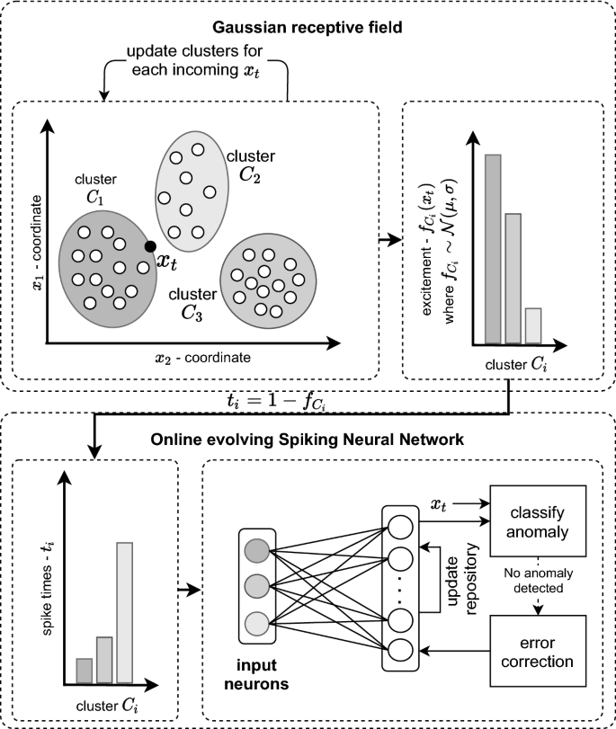
Illustration of multivariate online evolving SNN model (OeSNN-D)

The models were implemented with Cython (Behnel et al. 2011). Wrapping the external C++ library as a Python extension allows an accelerated execution compared to a Python native implementation, which is especially beneficial for online and real-time data processing.

Table 1 Model overview

5.2 Evaluation benchmark

We use the Numenta Anomaly Benchmark (NAB) (Ahmad et al. 2017) to analyze the presented modifications of the OeSNN and to identify strengths and weaknesses of the adjustments. NAB consists of over 50 labeled real and artificial time series. All data including a comprehensive documentation are available as open source.¹ Much of the data consists of real time series data and comes from a variety of sources such as AWS server metrics, Twitter volumes, web click metrics, traffic data and more. These time series are mainly univariate records, which means that they are not suitable for our multivariate comparison and evaluation. Furthermore, the synthetic dataset contains only a few anomaly types. In order to allow a differentiated comparison of the performance of the different OeSNN modifications on the largest possible number of different outlier species, we added additional outlier types to the synthetically generated part of the Numenta dataset. Our extended benchmark data set, which is also shown in appendix A.1, contains outliers of the following categories: signal dropouts, signal drift, lower amplitude, higher amplitude, cycle dropout, single peaks, change of frequency, increase in noise and increase in amplitude. For the evaluation of multivariate time series the synthetic datasets are combined so that one outlier is present in one dimension, while the other dimensions use the anomaly-free synthetic signal.

5.3 Hyperparameter optimization

In the literature a wide range of different algorithms for the optimization of hyperparameters is presented (Yu and Zhu 2020; Bergstra et al. 2011). Many of these algorithms, such as grid search, use a relatively naive approach for the selection of hyperparameter optimization, which means that the effort for the optimization of the given parameters for high dimensional optimization problems can only be realized with massive computational resources. Furthermore, since the number of outliers in both the given artificially generated and real data belong to the minority class, it is not possible to fall back on a large data pool for hyperparameter optimization here. Therefore, it cannot be guaranteed that there is no overfitting of the parameters to a certain type of outlier, which could influence the generalization ability of the algorithms. In addition, in many real-world applications, outliers of the signal are not present for optimization, which presents further difficulties.

Due to the high number of hyperparameters of the OeSNN (see Appendix A.2) as well as the low number of test and validation data, we present in the following sections a technique to effectively select the hyperparameter candidates as well as an approach to optimize the hyperparameters without prior knowledge of the signal-specific outlier types.

5.3.1 Generation of validation data

In order to avoid overfitting of the model due to the small size of the data instances of the NAB dataset and to enable a method for optimizing the algorithm without prior knowledge of the signal-specific outlier types we investigate a method of optimization using only an artificially generated anomaly. For this purpose, we replace in one dimension of the anomaly-free signal a window slightly larger than one cycle with an artificially generated noise as illustrated in Fig. 5.

Fig. 5

Signal of the Numenta Anomaly Benchmark without anomaly (left) and the corresponding generated data (right) with inserted artificial noise, which is used for hyperparameter optimization

For the optimization of the model, we use the reconstruction error of the predicted signal on the artificially generated anomaly signal and the anomaly-free signal as a quality measure. In comparison to an optimization with only one real outlier type, this method provides consistently comparable or better generalization results (see A.5).

5.3.2 Efficient hyperparameter selection

In order to reduce the required number of hyperparameters to be tested and to minimize the required time for hyperparameter optimization we used the tree-structured parzen estimator (TPE) approach (Bergstra et al. 2011, 2013). We implement the optimization with the Python framework Optuna (Akiba et al. 2019). Here we optimize the hyperparameters in 1500 trials as shown in Table 2, of which 20% are initialized with random parameters. For the selection of the next parameters, 50 possible parameter configurations are randomly chosen per iteration, which is represented by the EI-candidates value in Table 2. On the basis of these configurations the expected improvement of the model is calculated. We run all iterations of the optimization algorithm sequentially on one thread to obtain reproducible results. We also initialize a random generator, which is used for the selection of the parameter candidates, with a constant seed. We consider the selection of the optimal hyperparameters ($\theta ^{*}$) as an optimization problem with constraint (cf. Eqs. (13) and (14)). The aim is to minimize the mean squared error between the reconstruction output ($\hat{\mathbf {y}}_{i}$) of the OeSNN algorithm with the artificially generated outlier ($\tilde{\mathbf {x}}_{i}$) as input and the original signal without outlier ($\mathbf {x}_{i}$) under the constraint that for less than $1\%$ of the data instances k none of the output neurons fires. Constraint Eq. (14) is necessary, since otherwise the best hyperparameters are found by simply reproducing the original data, which leads to an overfitting. Instead of $1\%$ any small value can be used to prevent overfitting.

Table 2 Parameters of the TPE algorithm for hyperparameter search

$$\begin{aligned}&\begin{array}{l@{{}={}}l} \theta ^{*} & \arg \min _{\theta } \frac{1}{k} \sum _{i=1}^{k}\left( \hat{\mathbf {y}}_{i} - \mathbf {x}_{i}\right) ^{2} \\ & \arg \min _{\theta } \frac{1}{k} \sum _{i=1}^{k}\left( \text {OeSNN}\left( \theta , \tilde{\mathbf {x}}_{i}\right) - \mathbf {x}_{i}\right) ^{2} \end{array} \end{aligned}$$

(13)

$$\begin{aligned}&\text {subject to } t_{\text {not fired}} < 0.01 \cdot k \end{aligned}$$

(14)

We perform this optimization task for each of the described OeSNN for the two-dimensional case. The respective search space for the hyperparameters can be looked up in the appendix A.2. The optimization results are then transferred to all other dimensions. Since the defined optimization criterion does not allow direct optimization of the window size parameter of the outlier score, we adjusted this parameter manually after the optimization. Here we selected a value as a trade off between a high sensitivity to changes in the signal and an overall low variance of the score.

5.4 Model evaluation

To evaluate the algorithms for detecting anomalies in a streaming context we perform four quantitative benchmarks for the created variations of the OeSNN algorithm. They consist of a runtime analysis of the models, which will be examined in the following with regard to an increasing number of data points as well as an increasing number of dimensions. In addition, we investigated the anomaly detection with regards to the suitability for detecting anomalies in high-dimensional data as well as the detection of various types of anomalies. The exact configuration of the benchmarks is shown in Table 3.

Table 3 Configuration of benchmarks to evaluate the algorithms

To estimate the performance of the OeSNN in the context of online anomaly detection algorithms we used the SPIRIT algorithm according to Papadimitriou et al. (2005) as reference algorithm. In order to compare the OeSNN-D algorithm with deep learning methods as in Munir et al. (2019), we also evaluated the OeSNN-D algorithm on a different dataset, the Yahoo Webscope dataset and compare it to the results obtained in Munir et al. (2019). For all experiments the hyperparameters, as determined in the previous section, are provided in the appendix A.3.

Selecting a suitable metric for the evaluation of the anomaly recognition rate of the algorithms is an important component. The goal is to select a suitable metric that is invariant with respect to an imbalance between normal data points and outliers and provides a suitable basis for comparing the model with other algorithms. For the quantitative determination of the performance of the algorithms we use the F1 score [Eq. (15)] on the benchmark datasets. Although it is used much less frequently in the scientific literature than the accuracy score (Hossin and Sulaiman 2015), it is especially suitable for classifications with unequally weighted classes (Jeni et al. 2013). In addition, the F1 score can be found in a number of other publications in the field of anomaly detection (Macia̧g et al. 2021; Däubener et al. 2019; Munir et al. 2019), which facilitates a comparison of the algorithms:

$$\begin{aligned} F_{1} = 2 \cdot \frac{P \cdot R}{P+R} \end{aligned}$$

(15)

The F1 score is calculated on the basis of the fraction of correctly predicted positive instances from all positive predictions P (Precision) and the fraction of correctly predicted positive instances from all positive instances R (Recall) (Hossin and Sulaiman 2015):

$$\begin{aligned} \text {Precision} (P)= & {} \frac{t_{p}}{t_{p} + f_{p}} \end{aligned}$$

(16)

$$\begin{aligned} \text {Recall} (R)= & {} \frac{t_{p}}{t_{p}+f_{n}} \end{aligned}$$

(17)

where $t_{p}$ are the correctly classified outliers, $f_{n}$ unrecognized outliers and $f_{p}$ data instances which were incorrectly classified as outliers.

5.5 Experimental determination of runtimes

To analyze runtime, we make use of an experimental evaluation instead of a theoretical analysis of the runtime of the algorithm via O-notation. To ensure the comparability of the results, we executed the tests sequentially one after the other on a defined system (i9-9900k, 32 GB DDR4 RAM, Ubuntu 20.04.1 LTS) without any additional load that could have a negative impact on the results. In order to obtain the most precise results possible, the selection of the timer module also has an important role. Special attention should be paid to a high temporal resolution. For this purpose, we use the process_time_ns function from standard Python library (Stinner 2017) which has the highest temporal resolution with 1 nano second. To compensate the inaccuracies due to the parallel occurring load or further inaccuracies in the determination of the runtime, all experiments for the analysis of the running time are performed with a sample size of $m=20$.

5.5.1 Influence of number of data points

Based on the tests performed regarding the change in runtime with increasing number of data points, it can be determined that the OeSNN-D version of the algorithm scales best with new incoming data points when only 2 clusters are required for the distribution of the multivariate Gaussian recipe fields as shown in Fig. 6. The runtime of the algorithm for $10^{6}$ data points is only 40% of that of OeSNN-A. Also compared to the SPIRIT reference algorithm as well as the other variants of the OeSNN, the runtime of the algorithm is in a very good range. Especially noticeable is the improvement of the OeSNN from variant C to variant D. The Spiking Neural Network with preceding multivariate GRF requires a multiple of the runtime of the final model. This reduction of the runtime is described by Wang et al. (2017) and is also reinforced by the reduced number of input neurons.

Fig. 6

Runtime of the investigated algorithms with increasing number of data points

Moreover, we observe that the adapted scoring system, which enables a real-value classification of outliers, can achieve a significant improvement in runtime (cf. OeSNN-A and OeSNN-B).

5.5.2 Influence of dimensionality of the input data

As the dimensionality of the data increases, the number of processing points also increases, which makes preserving real-time capability almost impossible. Among the algorithms as well as their variations we could prove that the variants (OeSNN-A; OeSNN-B) that allow processing of multivariate data only by executing several instances with increasing dimensionality do not benefit from the correlation of the data dimensions (see Fig. 7). With the OeSNN-B variant of the algorithm, which uses an adapted online-capable variant of the Numenta outlier score. However, we could observe a significant improvement compared to variant OeSNN-A.

Fig. 7

Runtime of the investigated algorithms with increasing number of dimensions

All other variants of the algorithm (OeSNN-C, OeSNN-D), which are based on coding multivariate data using the multidimensional GRF, scale significantly better with increasing dimensionality as can be seen from Fig. 7. The runtime of the OeSNN-D from the one-dimensional to the twenty-dimensional input signal increases by a factor of about 3.5, whereas the runtime of the initial OeSNN-A increases by a factor of 21.

5.6 Anomaly detection of different algorithms

In addition to the runtime, a high detection rate of anomalies in time series is a fundamental requirement. In the following, this will be analyzed and discussed with regard to the general detection rate for several dimensions and the average detection rate of different types of anomaly in the NAB dataset. For the evaluation, we used the F1 score described in Sect. 5.4. The complete results of the evaluation are provided in Appendix A.5. Furthermore in order to evaluate the new OeSNN-D algorithm on a different dataset we investigate in Sect. 5.6.3 its performance on the Yahoo webscope dataset, which consists of four groups of benchmark datasets A1, A2, A3, A4. These datasets are also investigated in Munir et al. (2019) with a deep learning algorithm.

5.6.1 Anomaly detection and increasing dimensionality of the data

Our analysis show that the average F1 score of the OeSNN-D model for the tested NAB dataset with dimensions (2–4) gives better results than all compared models (see Table 4). Remarkable is the increase of the average F1 score compared to the initial model (OeSNN-A) by 0.36, due to the different outlier score calculation. Furthermore, we show that by coding the multidimensional data for the models OeSNN-C and OeSNN-D, the recognition rate of the algorithms can be further improved.

Table 4 Average F1 score of the models for detecting anomalies across all anomaly types of the NAB dataset

Comparing the models OeSNN-B, OeSNN-C and OeSNN-D as in Table 4, we notice that the F1 score increases with each version. The results in Table 4 are in some cases also astonishing since with the implementation of the GRF the higher dimensional cases do have a better F1 score than the one dimensional case. The reason is that several outlier types as for example cycle dropouts and change of frequency perform really bad when calculating the F1 score in the one dimensional case for OeSNN-C and OeSNN-D (see Sect. A.4). But they perform really good in the higher dimensional case, when the anomaly occurs only in one and not in all dimensions. In this case the multidimensional data points of the anomalies lie in another region than the normal data points, which makes it easier for the GRF to detect them. This of course shows that our OeSNN-D model has its real strength in the multivariate case.

5.6.2 Detection of different outlier types in the NAB dataset

As shown in Table 5, the OeSNN-D model achieves the highest F1 score for most anomaly types in the NAB dataset. This includes all categories except for the outlier types cycle dropouts, increase in noise and increase in amplitude (see Appendix A.5). However, for the categories cycle dropouts and increase in amplitude, the model is with a deviation of 0.01 and 0.05, respectively, very close to the highest achieved F1 score. We identify a deficit of the OeSNN-D model compared to the reference algorithm (SPIRIT) in the outlier category increase in noise.

Table 5 Average F1 score of the models for detection of the anomaly types of the NAB dataset averaged over the dimensions 2-4

As previously with the analysis of the recognition rate in Sect. 5.6.1, we also see a step-by-step improvement with increasing dimensionality of the data for the models OeSNN-C and OeSNN-B, whereby we could also prove the positive influence of the individual modifications on the performance of the final model (OeSNN-D). For the case of increase in noise the principal component in the SPIRIT algorithm is not able to converge, therefore the algorithm detects an anomaly. Whereas in the OeSNN algorithms the increasing noise oscillates around the mean value of a Gaussian receptive field which leads to similar spike values such that no anomaly is detected.This also illustrates the different nature of both algorithms. Whereas SPIRIT detects outliers, whenever the principal component of a multivariate data stream changes, our OeSNN-D algorithm detects outliers if the clusters of multidimensional datasets change in length or form.

5.6.3 Anomaly detection in the Yahoo Webscope dataset

The main focus of the newly developed anomaly detection algorithm OeSNN-D is to detect online anomalies in multivariate time series of periodic or seasonal processes i.e. in production processes. The results in Sect. 5.6.2 show that the performance of the OeSNN-D algorithm is very good if structural anomalies are considered. In this section we evaluate the Yahoo Webscope dataset, a publicly available data set released by Yahoo Labs. It consists of 367 real and synthetic time series with point anomaly labels. Each time series contains 1420 to 1680 instances. It is divided into four sub-benchmarks namely A1 Benchmark, A2 Benchmark, A3 Benchmark and A4 Benchmark. Most of the anomalies in the Yahoo Webscope datasets are point anomalies, which means there is only one anomalous time series index in a certain neighbourhood. The Yahoo Webscope dataset was also considered in Munir et al. (2019), where deep learning methods were applied to detect anomalies. We evaluated the anomalies of the Yahoo Webscope dataset as it was done in Munir et al. (2019) by determining the hyperparameter for every sub benchmark A1, A2, A3, A4 seprately (see Appendix A.3) the results can be seen in Table 6.

Table 6 Average F1 score for the Yahoo Webscope dataset in comparison with the results in Munir et al. (2019)

Although the F1 score of the OeSSN-D algorithm can not compete with the deep learning models of DeeptAnT, it is obtains most of the time better results than other none deep learning algorithms. Since the main focus of our algorithm lies in the online detection of anomalies without a training phase, the results are very promising also for this data set.

However, since most of the anomalies in the Yahoo Webscope dataset are point anomalies, a separate algorithm for point anomalies can be developed and, in the best case, put into parallel operation with the OeSNN-D algorithm. Most point anomalies can be detected by an algorithm which calculates the differences of successive times series values $\varDelta x_t= x_t-x_{t-1}$ in a certain sliding window $w_{1}$ with length $|w_1|$ and compare them to the directly following differences of a very small sliding window $w_{2}$ of length $|w_2|$. Thus,

$$\begin{aligned} w_{1}= & {} \{\varDelta x_{t-|w_1|-|w_2|}, \varDelta x_{t-|w_1|-|w_2|+1},...,x_{t-|w_2|}\} \text{ and }\\ w_{2}= & {} \{\varDelta x_{t-|w_2|}, \varDelta x_{t-|w_2|+1},...,x_{t}\}. \end{aligned}$$

A point anomaly is detected whenever

$$\begin{aligned} |\varDelta x_t-{\overline{w}}_1|\ge \sigma _{w_1}\cdot \epsilon \text{ and } |\sum _{v\in w_2}v|<|\sigma _{w_1}\cdot (\epsilon -0.5)|, \end{aligned}$$

where $\sigma _{w_1}$ denotes the standard deviation and ${\overline{w}}_1$ the mean of $w_1$. The parameters $\epsilon , |w_1|$ and $|w_2|$ are hyperparameters, which are set to $\epsilon =4.5$, $|w_1|=32$ and $|w_2|=4$. Evaluating the Yahoo Webscope with this algorithm detects most of the point anomalies. The reuslts are shown in Table 7.

Table 7 Average F1 score for the point anomaly detector on the Yahoo Webscope dataset in comparison with the results in Munir et al. (2019)

6 Conclusion

In this paper we introduce an online capable algorithm to efficiently detect anomalies in multivariate time series. We therefore use an online Spiking Neural Network architecture with a data efficient technique for coding higher-dimensional data using Multidimensional Gaussian Receptive Fields (GRF) as well as advanced learning methods for improved multidimensional anomaly detection.

In the evaluation of several versions of multidimensional online Spiking Neural Networks (OeSNN-A; OeSNN-B; OeSNN-C; OeSNN-D) using the Numenta Anomaly Benchmark (NAB) and the Yahoo Webscope dataset we prove that several modifications of the initial OeSNN algorithm according to Maciąg et al. (2021) significantly improve the general suitability for outlier detection in higher dimensional ($n \ge 2$) data and the detection of specific outlier types while requiring consistently less runtime than the initial algorithm. In addition, we determine a better detection result for almost all outlier types compared to the reference SPIRIT algorithm. Our new algorithm shows deficits only in the outlier types increase in noise and individual peaks. Individual peaks or point anomalies are hard to detect with our algorithm, but they can be detected with a different algorithm as we showed in Sect. 5.6.3.

To assess the suitability of the adapted OeSNN further, we will investigate more complex signal types from different application domains. Thus, we also check whether our algorithm meets the requirements of Wu and Keogh (2021). The authors there question the usage of deep learning models for anomaly detection in time series. That is why we believe that spiking neural networks and specifically our OeSNN-D model might be one of the best ways to detect anomalies, which are not trivial and can be weed out with two lines of code, in multivariate streaming times series. As pointed out in this paper and in Wu and Keogh (2021) as well, a lot of the point anomalies of the Yahoo Webscope dataset can be detected with a really simple algorithm. The focus in this paper is however to detect structural changes in multivariate times series and also to categorize the different type of anomalies whether they are detectable by our algorithm or not. In order to further strengthen the online capability of our algorithm the number of required hyperparameters must be reduced in further work or some new insights for transferring existing hyperparameters between different application domains must be established.

A Appendix

1.1 A.1 Signal categories of the extended Numenta Anomaly Benchmark

For adding additional anomalies which are not contained in the original NAB dataset, we used the time series of the NAB dataset and modified it in an adequate way. The time series signal dropouts, higher amplitude, lower amplitude and cycle dropout are from the original NAB dataset. For signal drift we added a linear function to the original time series from a certain time step onwards, for single peaks we added a few peaks to the time series, for change of frequency we divided the frequency of the original NAB time series by two from a certain time step onwards, for increase in noise we added an additional gaussian noise to the original NAB dataset and for increase in amplitude we added a rectangle function with increasing amplitude from a certain time point onwards (Fig. 8).

Fig. 8

Signal categories of the extended Numenta Anomaly Benchmark

1.2 A.2 Hyperparameter search space

See Table 8.

Table 8 Hyperparameter search space with p as number of data points for a signal period

1.3 A.3 Determined hyperparameters for the evaluation of the datasets

See Tables 9, 10, 11, 12, 13 and 14.

Table 9 Hyperparameters on the modified NAB dataset for the OeSNN-A model

Table 10 Hyperparameters on the modified NAB dataset for the OeSNN-B model

Table 11 Hyperparameters on the modified NAB dataset for the OeSNN-C model

Table 12 Hyperparameter on the modified NAB dataset for the OeSNN-D model

Table 13 Hyperparameter on the Yahoo Webscope dataset for the OeSNN-D model

Table 14 Hyperparameters on the modified NAB dataset for the SPIRIT model

1.4 A.4 Anomaly detection results

See Tables 15, 16 and 17.

Table 15 Average F1 score to detect the anomaly types of the NAB dataset for one dimension

Table 16 Average F1 score to detect the anomaly types of the NAB dataset for two dimensions

Table 17 Average F1 score to detect the anomaly types of the NAB dataset for four dimensions

1.5 A.5 Visualization of the outlier scores for different algorithms

See Figs. 9 and 10.

Fig. 9

Visualization of the outlier score of the OeSNN models and the SPIRIT reference algorithm on the adapted NAB dataset with four dimensions

Fig. 10

Visualization of the outlier score of the OeSNN models and the SPIRIT reference algorithm on the adapted NAB dataset with four dimensions

References

Aggarwal, C. (2013). Outlier analysis. New York, NY: Springer-Verlag.
Ahmad, S., Lavin, A., Purdy, S., & Agha, Z. (2017). Unsupervised real-time anomaly detection for streaming data. Neurocomputing. https://doi.org/10.1016/j.neucom.2017.04.070
Akiba, T., Sano, S., Yanase, T., Ohta, T., & Koyama, M. (2019). Optuna: A next-generation hyperparameter optimization framework. In: Proceedings of the 25th ACM SIGKDD International Conference on Knowledge Discovery and Data Mining, Association for Computing Machinery, New York, NY, USA, KDD ’19, pp. 2623–2631, https://doi.org/10.1145/3292500.3330701.
Amirshahi, A., & Hashemi, M. (2019). Ecg classification algorithm based on stdp and r-stdp neural networks for real-time monitoring on ultra low-power personal wearable devices. IEEE Transactions on Biomedical Circuits and Systems, 13(6), 1483–1493. https://doi.org/10.1109/tbcas.2019.2948920.
Bear, M., Seidler, L., Engel, A., Held, A., Connors, B., Hornung, C., et al. (2016). Neurowissenschaften: Ein grundlegendes Lehrbuch für Biologie. Springer, Berlin Heidelberg: Medizin und Psychologie.
Behnel, S., Bradshaw, R., Citro, C., Dalcin, L., Seljebotn, D. S., & Smith, K. (2011). Cython: The best of both worlds. Computing in Science & Engineering, 13(2), 31–39.
Bergstra, J., Bardenet, R., Bengio, Y., & Kégl, B. (2011). Algorithms for hyper-parameter optimization. In Proceedings of the 24th international conference on neural information processing systems, Curran Associates Inc., Red Hook, NY, USA, NIPS’11, pp. 2546–2554.
Bergstra, J., Yamins, D., & Cox, DD. (2013). Making a science of model search: Hyperparameter optimization in hundreds of dimensions for vision architectures. In Proceedings of the 30th international conference on international conference on machine learning, Volume 28, JMLR.org, ICML’13, pp. I-115–I-123.
Bianco, A., Garcia Ben, M., Martínez, E., & Yohai, V. (2001). Outlier detection in regression models with arima errors using robust estimates. Journal of Forecasting,20. https://doi.org/10.1002/for.768.
Bing, Z., Meschede, C., Huang, K., Chen, G., Rohrbein, F., Akl, M., & Knoll, A. (2018a). End to End Learning of Spiking Neural Network Based on R-STDP for a Lane Keeping Vehicle. Proceedings—IEEE international conference on robotics and automation pp. 4725–4732. https://doi.org/10.1109/ICRA.2018.8460482.
Bing, Z., Meschede, C., Röhrbein, F., Huang, K., & Knoll, A. C. (2018). A survey of robotics control based on learning-inspired spiking neural networks. Frontiers in Neurorobotics, 12, 35. https://doi.org/10.3389/fnbot.2018.00035.
Breunig, MM., Kriegel, HP., Ng, RT., & Sander, J. (2000). Lof: Identifying density-based local outliers. In Proceedings of the 2000 ACM SIGMOD international conference on management of data, association for computing machinery, New York, NY, USA, SIGMOD ’00, pp. 93–104. https://doi.org/10.1145/342009.335388, https://doi.org/10.1145/342009.335388.
Chalapathy, R., & Chawla, S. (2019). Deep learning for anomaly detection: A survey. arXiv:1901.03407.
Däubener, S., Schmitt, S., Wang, H., Bäck, T., peter, krause. (2019). Large anomaly detection in univariate time series: An empirical comparison of machine learning algorithms. In 19th Industrial conference on data mining ICDM 2019, Unknown.
Demertzis, K., Iliadis, L., & Spartalis, S. (2017). A spiking one-class anomaly detection framework for cyber-security on industrial control systems. In G. Boracchi, L. Iliadis, C. Jayne, & A. Likas (Eds.), Engineering applications of neural networks (pp. 122–134). Cham: Springer International Publishing.
Demertzis, K., Iliadis, L., & Bougoudis, I. (2019). Gryphon: A semi-supervised anomaly detection system based on one-class evolving spiking neural network. Neural Computing and Applications. https://doi.org/10.1007/s00521-019-04363-x.
Fu, X., Luo, H., Zhong, S., & LIN L,. (2019). Aircraft engine fault detection based on grouped convolutional denoising autoencoders. Chinese Journal of Aeronautics,32(2), 296–307. https://doi.org/10.1016/j.cja.2018.12.011, http://www.sciencedirect.com/science/article/pii/S1000936119300238.
Geiger, A., Liu, D., Alnegheimish, S., Cuesta-Infante, A., & Veeramachaneni, K. (2020). Tadgan: Time series anomaly detection using generative adversarial networks. arXiv:2009.07769.
Gerstner, W., & Kistler, W. M. (2002). Spiking neuron models: Single neurons, populations, plasticity. Cambridge University Press. https://doi.org/10.1017/CBO9780511815706.
Goodfellow, I., Bengio, Y., & Courville, A. (2016). Deep learning. MIT Press.
Gühring, G., Baum, C., Kleschew, A., & Schmid, D. (2019). Anomalie-erkennung. atp magazin, 61, 66. https://doi.org/10.17560/atp.v61i5.2380.
Hau, M., & Tong, H. (1989). A practical method for outlier detection in autoregressive time series modelling. Stochastic Hydrology and Hydraulics, 3, 241–260. https://doi.org/10.1007/BF01543459.
Hopkins, M., García, G., Bogdan, P., & Furber, S. (2018). Spiking neural networks for computer vision. Interface Focus, 8, 20180007. https://doi.org/10.1098/rsfs.2018.0007.
Hossin, M., & Sulaiman, M. (2015). A review on evaluation metrics for data classification evaluations. International Journal of Data Mining & Knowledge Management Process, 5, 01–11. https://doi.org/10.5121/ijdkp.2015.5201.
Jeni, LA., Cohn, JF., & De La Torre, F. (2013). Facing imbalanced data–recommendations for the use of performance metrics. In 2013 Humaine association conference on affective computing and intelligent interaction, pp. 245–251.
Kasabov, N. (2006). Evolving connectionist systems: The knowledge engineering approach. Berlin, Heidelberg: Springer-Verlag.
King, A. (2012). Online k-means clustering of nonstationary data. Prediction Protect Report. p. 11.
Kriegel, HP., Kröger, P., Schubert, E., & Zimek, A. (2009). Loop: Local outlier probabilities. In Proceedings of the 18th ACM conference on information and knowledge management, association for computing machinery, New York, NY, USA, CIKM ’09, pp. 1649-1652. https://doi.org/10.1145/1645953.1646195, https://doi.org/10.1145/1645953.1646195.
Lapicque, L. (1907). Recherches quantitatives sur l’excitation électrique des nerfs traitée comme une polarisation. Journal de Physiologie et de Pathologie Générale, 9, 620–635. https://doi.org/10.1007/s00422-007-0189-6.
Lobo, J. L., Lan̄a, I., Del Ser, J., Bilbao, MN., & Kasbov, N. (2018). Evolving Spiking Neural Networks for online learning over drifting data streams. Neural Networks,108, 1–19. https://doi.org/10.1016/j.neunet.2018.07.014.
Lobo, J. L., Javier, D. S., Albert, B., & Nikola, K. (2020). Spiking Neural Networks and online learning: An overview and perspectives. Neural Networks, 121, 88–100. https://doi.org/10.1016/j.neunet.2019.09.004.
Li, D., Chen, D., Jin, B., Shi, L., Goh, J., & Ng, S. K. (2019). Mad-gan: Multivariate anomaly detection for time series data with generative adversarial networks. In I. V. Tetko, V. Kůrková, P. Karpov, & F. Theis (Eds.), Artificial neural networks and machine learning—ICANN 2019: Text and time series (pp. 703–716). Cham: Springer International Publishing.
Li, Y., Lu, A., Wu, X., & Yuan, S. (2019b). Dynamic anomaly detection using vector autoregressive model. Springer International Publishing, pp. 600–611. https://doi.org/10.1007/978-3-030-16148-4_46.
Lindeberg, T. (2013). A computational theory of visual receptive fields. Biological Cybernetics, 107(6), 589–635.
Maas, W. (1997). Networks of spiking neurons: The third generation of neural network models. Trans Soc Comput Simul Int, 14(4), 1659–1671.
Macia̧g, P. S., Kryszkiewicz, M., Bembenik, R., Lobo, J. L., & Ser, J. D. (2021). Unsupervised anomaly detection in stream data with online evolving spiking neural networks. Neural Networks,139, 118–139.
Mahajan, M., Nimbhorkar, P., & Varadarajan, K. (2012). The planar k-means problem is NP-hard. Theoretical Computer Science, Elsevier, 442, 13–21.
Malhotra, P., Ramakrishnan, A., Anand, G., Vig, L., Agarwal, P., & Shroff, G. (2016). Lstm-based encoder-decoder for multi-sensor anomaly detection. ArXivarXiv:1607.00148
Moayedi, H., & Masnadi-Shirazi, M. (2008). Arima model for network traffic prediction and anomaly detection. In 2008 International symposium on information technology, Vol. 4, pp. 1–6.
Munir, M., Siddiqui, S. A., Dengel, A., & Ahmed, S. (2019). Deepant: A deep learning approach for unsupervised anomaly detection in time series. IEEE Access, 7, 1991–2005.
Panuku, L. N., & Sekhar, C. C. (2008). Region-based encoding method using multi-dimensional gaussians for networks of spiking neurons. In M. Ishikawa, K. Doya, H. Miyamoto, & T. Yamakawa (Eds.), Neural information processing (pp. 73–82). Heidelberg: Springer, Berlin Heidelberg, Berlin.
Papadimitriou, S., Sun, J., & Faloutsos, C. (2005). Streaming pattern discovery in multiple time-series. In Proceedings of the 31st international conference on very large data bases, VLDB endowment, VLDB ’05, pp. 697–708.
Pokrajac, D., Lazarevic, A., & Latecki, L. J. (2007). Incremental local outlier detection for data streams. In 2007 IEEE symposium on computational intelligence and data mining, pp. 504–515.
Schliebs, S., & Kasabov, N. (2013). Evolving spiking neural networks: A survey. Evolving Systems,4. https://doi.org/10.1007/s12530-013-9074-9.
Schuman, CD., Potok, TE., Patton, RM., Birdwell, JD., Dean, ME., Rose, GS., & Plank, JS. (2017). A survey of neuromorphic computing and neural networks in hardware. arXiv:1705.06963.
Shukla, R., & Sengupta, S. (2020). Scalable and robust outlier detector using hierarchical clustering and long short-term memory (lstm) neural network for the internet of things. Internet of Things, 9, 100167. https://doi.org/10.1016/j.iot.2020.100167.
Stinner, V. (2017). Pep 564 – add new time functions with nanosecond resolution. https://www.python.org/dev/peps/pep-0564/. [Online; accessed 16 August 2020].
Taddei, A., Distante, G., Emdin, M., Pisani, P., Moody, G. B., Zeelenberg, C., & Marchesi, C. (2000). European st-t database. https://doi.org/10.13026/C2D59Z.
Thorpe, S., & Gautrais, J. (1998). Rank order coding. Computational Neuroscience: Trends in Research pp. 113–118. https://doi.org/10.1007/978-1-4615-4831-7_19.
Wang, J., Belatreche, A., Maguire, L. P., & McGinnity, T. M. (2017). Spiketemp: An enhanced rank-order-based learning approach for spiking neural networks with adaptive structure. IEEE Transactions on Neural Networks and Learning Systems, 28(1), 30–43.
Watts, M. (2009). A decade of Kasabov’s evolving connectionist systems: A review. Systems, Man, and Cybernetics, Part C: Applications and Reviews, IEEE Transactions on, 39, 253–269. https://doi.org/10.1109/TSMCC.2008.2012254.
Welford, B. P. (1962). Note on a method for calculating corrected sums of squares and products. Technometrics, 4(3), 419–420. https://doi.org/10.1080/00401706.1962.10490022.
Wu, J., Yılmaz, E., Zhang, M., Li, H., & Tan, K. C. (2020). Deep spiking neural networks for large vocabulary automatic speech recognition. Frontiers in Neuroscience, 14, 199. https://doi.org/10.3389/fnins.2020.00199.
Wu, R., & Keogh, E. (2021). Current time series anomaly detection benchmarks are flawed and are creating the illusion of progress. IEEE Transactions on Knowledge and Data Engineering. https://doi.org/10.1109/TKDE.2021.3112126.
Wysoski, S. G., Benuskova, L., & Kasabov, N. (2006). On-line learning with structural adaptation in a network of spiking neurons for visual pattern recognition. In S. D. Kollias, A. Stafylopatis, W. Duch, & E. Oja (Eds.), Artificial neural networks—ICANN 2006 (pp. 61–70). Heidelberg: Springer, Berlin Heidelberg, Berlin.
Wysoski, S. G., Benuskova, L., & Kasabov, N. (2008). Adaptive spiking neural networks for audiovisual pattern recognition (pp. 406–415). Berlin, Heidelberg: Springer-Verlag.
Xing, L., Demertzis, K., & Yang. (2019). Identifying data streams anomalies by evolving spiking restricted boltzmann machines. Neural Computing and Applications,31, 1–15. https://doi.org/10.1007/s00521-019-04288-5c.
Yu, T., & Zhu, H. (2020). Hyper-parameter optimization: A review of algorithms and applications. arXiv:2003.05689.
Zhang, G. (2003). Time series forecasting using a hybrid Arima and neural network model. Neurocomputing, 50, 159–175. https://doi.org/10.1016/S0925-2312(01)00702-0.
Funding
Open Access funding enabled and organized by Projekt DEAL. No funding was received to assist with the preparation of this manuscript.
Author information
Authors and Affiliations
Contributions
Dennis Bäßler, Tobias Kortus and Gabriele Gühring contributed in an equal way to this paper.
Corresponding author
Ethics declarations
Conflict of interest
The authors declare that they have no conflict of interest.
Ethics approval
Not Applicable.
Consent for publication
Upon acceptance we will either grant the Publisher an exclusive license to publish the article or will transfer copyright of the article to the Publisher.
Additional information
Editor: Joao Gama.
Publisher's Note
Springer Nature remains neutral with regard to jurisdictional claims in published maps and institutional affiliations.