A deep learning approach using natural language processing and time-series forecasting towards enhanced food safety

Abstract

In various application domains/sectors, data collected from the respective industries are complemented with open data providing added value to the overall analysis and decision making process. Open data refer to weather data, transportation information, stock/investment products prices, or even health-related data. One of the application domains that could harvest the added-value of analytics (including open-data) refers to the food industry and more specifically the decisions related to food recalls. The collected data can be analyzed in real-time through Artificial Intelligence techniques and obtain insights about potential unsafe goods and products. These insights are exploited to drive decision making, such as which goods are more probable to be harmful in the near future and subsequently optimize the food supply chain. The latter reflects the overall food recall process monitoring and is enhanced through a data-driven forecasting approach. This provides actionable insights regarding the enhancement of the food safety across the food supply chain given that goods and products can become unsafe for plenty of reasons, such as mislabeling allergens, contamination etc. To address this challenge, this paper introduces a deep learning approach leveraging Natural Language Processing and Time-series Forecasting techniques, to monitor and analyze the risk associated with each food product category and the corresponding potential recalls. Furthermore, we propose a technique that exploits reinforcement learning to utilize historical recall announcements of food products for predicting their future recalls, thus providing insights to food companies regarding upcoming trends in food recalls that can lead to timely recalls. We also evaluate and demonstrate the effectiveness and added-value of the proposed approaches through a real-world scenario that yields promising results. While several techniques/models have been analyzed and applied to address the challenge of food recall predictions, the usage of analogous/surrogate data has also been studied and evaluated towards more accurate outcomes.

1 Introduction

Food safety has attracted considerable public concern and press attention in recent years. Global associations such as the FDA (‘Food and Drug Administration’) or the WHO (‘World Health Organization’) pose very strict regulations throughout the supply chain in order to assess and monitor the risk of food safety (FAO/WHO, 2007). That makes sense, given the fact that many products found in the food-marketplace may be harmful not only for individuals but also for the general economy and health system (Nyachuba 2010; Devlin et al. 2018).

One of the most efficient methods towards food safety is the removal of food products, after they have been characterized as harmful, from the market at any stage of the supply chain, including those that are possessed by the consumers. This process is widely known as food recall. There are several reasons that may lead to a product being characterized as unsafe or harmful, with the most prevalent of them being the existence of undeclared allergens (Luo et al. 2021) and the contamination of specific food categories such as meat and poultry where harmful bacteria (Listeria, Salmonella, and Escherichia coli) (Zhao and Liu 2008) can be found.

At this moment, the procedure of quality assessment of food products is a tedious and time-consuming task due to the lack of homogeneity in recall announcements from the different organisations related to food safety worldwide. Of course, time is of the essence in this case considering that those products can be consumed during this process (Marvin et al. 2017). Therefore, it is vital to have a reliable system for early detection or even prediction of unsafe foods in order to prevent outbreaks and serious harm to the public. This is a challenge of utmost importance, that the research community related to food safety should focus on, as it is costing global economies billions (Gendel and Zhu 2013; Devlin et al. 2018). In summary the problem of food safety is an ever-changing one as new threats show up yearly putting to the test the current ways of food management. Besides being a tremendous challenge, it heavily impacts human lives. For example, according to WHO the Unsafe food causes more than 200 diseases—ranging from diarrhea to cancers. It is estimated that almost 1 in 10 people in the world—fall ill after eating contaminated food and 420.000 die every year, resulting in the loss of 33 million healthy life years (DALYs). Additionally, the monetary cost is high. Approximately 110 billion dollars is lost every year in productivity and medical expenses resulting from unsafe food in low- and middle- income countries. Moreover, according to the United States Department of Agriculture (USDA), food-borne illness costs the US economy$10-83 billion per year (Nyachuba 2010).

This paper addresses the emerging challenge of food-safety by introducing a data-driven approach to facilitate timely decision making for food recalls. In this context, the operational objective is twofold:

• 1. Timely food recalls based on efficient classification of each recall according to the underlying product. Providing a sound approach for how unstructured text data retrieved from heterogeneous sources can be transformed and classified using NLP methods and represented in the time domain as time-series enabling the exploit of the forecasting method.

• 2. Systematically forecast recalls based on historical data applied for each general product category. It is worthwhile mentioning that the latter task is the one described in the conference paper presented in Makridis et al. (2020). The aforementioned paper addressed mainly the food recalls forecasting task by applying and comparing different probabilistic Deep Learning and Reinforcement Learning methods. This is extended towards both the introduction of a meta-model enabling a hybrid implementation and the utility of surrogate data as a dataset enrichment approach.

While the scientific contributions that support and extend the proposed solution can be briefly summarised in terms of added value, as the proposed approach enables:

• (i) continuous optimisation of the model (and as a result of its outcomes as well) based on the utilization of an RL technique with specific re-training intervals for the NER model,

• (ii) enhanced model outcomes due the usage of surrogate data that enrich the dataset and contribute to better generalization of the proposed model,

• (iii) best-fit utilization of different models towards improved outcomes (and decision making) due to the exploitation of the proposed hybrid approach for selecting the best model for time-series forecasting.’

In this case, to accurately learn domain-specific knowledge extracted by short texted food recalls we built the proposed approach on top of spaCy (Honnibal and Montani 2017). SpaCy is a python library used for Natural Language Processing tasks providing an abstraction facilitating the solution of such tasks. One of the provided architectures uses deep neural networks (DNNs), specifically a similar architecture to iterated dilated convolutional neural networks with fast token encoders (Strubell et al. 2017), which have been reported to be successful in various Natural language processing (NLP) tasks such as word embeddings (Bengio et al. 2007; Mikolov et al. 2013), part-of-speech tagging (Tsuboi 2014), parsing (Socher et al. 2010, 2012), Named Entity Recognition—NER (Hammerton 2003). While research shows that pre-trained word embeddings can improve accuracy on NLP tasks (Pennington et al. 2014; Mikolov et al. 2013; Lebret and Collobert 2013) there was none pre-trained model for product entities making necessary the training of a new one. Given the nature of the food-related dataset regarding the text classification task, NER methodology was applied, considering the product as entities. Generally a named entity is a word or a phrase that clearly identifies one item from a set of other items that have similar attributes. Examples of named entities are organization, person, and location names in general domain; gene, protein, drug and disease names in biomedical domain (Li et al. 2020).

As far as the second aim of the proposed approach, i.e. forecasting of potential food recalls is concerned, time-series analysis could also be exploited, which is motivated by the challenge of reducing future uncertainty. Utility across different domains, denotes that the extraction of useful knowledge via temporal data is an active research area (Fu 2011). The methods for time-series prediction rely on historical data since they include intrinsic patterns that convey useful information for the future description of the phenomenon under investigation. In this case deep learning techniques were utilized to provide information regarding the risk associated with food products and the potential recalls. The techniques mainly focus on time-series forecasting and reinforcement learning in order to predict the number of food incidents based on specific industry scenarios. Concerning this task, many challenges had to be addressed, the one with the greatest scientific impact was the usage of synthetically produced surrogate data as a way of enriching the original dataset to improve performance of deep learning models.

The remaining of the paper is structured as follows. Section 2 includes the background knowledge for NER and time-series forecasting needed for the reader to follow up the rest of the paper, Sect. 3 presents the related work in the area of study of this paper, while Sect. 4 delivers an overview of the proposed approach, introduces the overall architecture and details regarding the collection of the data streams and how these are utilised within the models. Section 5 presents experiments that have been conducted to demonstrate and evaluate the operation of the implemented algorithms. The performance of the proposed mechanisms is depicted in the results and evaluation section. Finally, Section 6 concludes with a discussion on future research and potentials for the current study.

2 Background

2.1 NER—sequence tagging

Named Entity Recognition (NER) is a subclass of Natural Language Processing (NLP) domain. It corresponds to the ability to identify the named entities in documents, and label them with one of entity type labels such as person, location or organisation. However, there is a long tail of entity labels for different domains. It is a common problem to come up with entity classes that do not fit the traditional four-class paradigm (PER, LOC, ORG, MISC). There are many methods of annotating text in order to be used for NER methods, those methods look promising for NER but still leave much room for improvements.

In Natural Language Processing (NLP), the task of sequence tagging/labelling is used to assign a categorical label to each term of the sentence/document. One of the most common tagging schemes is Part Of Speech tagging (POS) which assigns parts of speech to each word. While this can be addressed as a classification task of each word, the literature highlights that the dependencies between words carry useful information, and thus improving accuracy when included. Therefore, multiple approaches have been carried out such as using conditional random fields (Pfeiffer et al. 2020), LSTMs with and without the usage of ELMo (Embeddings from Language Models) and BERT. Besides the difference in approaches there exist a difference in tagging strategies with “BIOE” being the most popular one. In BIOE tagging strategy, ‘B’ represents the beginning of an attribute, ’I’ represents the inside of an attribute, ‘O’ represents the outside of an attribute, and ‘E’ represents the end of an attribute. Other popular tagging strategies include ”UBIOE” and ”IOB”. ”UBIOE” has an extra tag ’U’ representing the unit token tag that separates one-word attributes from multi-word ones. While for ”IOB” tagging, ’E’ is omitted since ’B’ and ’I’ are sufficient to express e boundary of an attribute.

2.2 Reinforcement learning for time-series

Reinforcement Learning can be broken down to three main categories: critic-only, actor-only, actor-critic (Zhang et al. 2020). It is out of the scope of this paper to analyze extensively each category. Since the proposed approach falls into the critic-only category it should be noted that in the critic-only approach the agent tries to learn a state-action value function Q or an approximation of Q in order to create a mapping ${S,A}\,\rightarrow \,v$ representing the appropriateness of a particular action given the state, where S and A are the state and action spaces accordingly. While there are many implementations falling into this category the most prominent is the deep Q-learning (DQN) with many improvements such as fixed Q-targets, double DQN’s, dueling DQN (DDQN) and Prioritized Experience Replay (PER) (Hessel et al. 2018). For this approach to work it is necessary to either have a discrete action space or discretise a continuous one with methods such as tile-coding (Sherstov and Stone 2005), coarse coding, function approximation etc.

Finally, given that the examined time-series case is a multi-step ahead prediction task, it should be mentioned that for time-series forecasting, the task of using observed time-series in the past to predict values in a look-ahead horizon gets proportionally harder as this horizon widens (Lai et al. 2018). Currently, multi-step ahead prediction tasks are achieved by two different ways. The first one, called independent value prediction, consists of training a direct model to predict the exact steps ahead. The second strategy, called iterative method, consists of repeating one-step ahead predictions to the desired horizon. The iterative prediction only uses one model to forecast all the horizons needed; the objective is to analyze a short sequence of data and try to predict the rest of the data sequence until a predefined time-step is reached. The main drawback of this approach is the cumulative nature of the error. The latter approach was leveraged for the proposed RL-based model, while the utillized probabilistic DNN time-series models followed the independent value prediction method.

2.3 Surrogate data

The first step of time-series forecasting is to reject the “white-noise” null hypothesis. Subsequently, if non-linear methods such as ML, DL and RL are to be used it is necessary to reject the null hypothesis regarding the existence of solely temporal linear correlations in the time-series. A statistically sound framework for the aforesaid test is that of surrogate data, sometimes known as analogous data. It refers to time-series data that reproduce various statistical properties like the autocorrelation structure of a measured data set. The null hypothesis is represented by the surrogate data which are compared with the original data under a non-linear discriminating statistic to reject or approve the null hypothesis. In this work the usage of surrogate data was twofold;

• 1. Test the non-linearity hypothesis.

• 2. Enrich existing dataset with the newly generated data.

The latter is proposed due to the nature of most deep learning models which can benefit from the increase both in diversity and volume of training data. The null hypothesis in our case is that the usage of analogous data will help the generalization of some if not all deep learning models in the case of time-series forecasting. Even though there are multiple methods to generate such data the IAAFT method (Dolan and Spano 2001) was chosen.

3 Related work

3.1 NER task

It is widely known that Deep Learning models have overtaken many NLP tasks because they may extract important features from word or character embeddings trained on large amounts of data and NER tasks follow this trend as well (Li et al. 2020). While this holds true, there is no pre-trained Language Model that can achieve SotA performance to supervised downstream tasks without the need of fine-tuning. There are many Language Models (LM) fine tuned in order to accomplish state of the art performance in a specific task and in a specific type of text in a specific language. A well-known paradigm of such language model achieving impressive results is SciBERT, a Bidirectional Encoder Representations from Transformers (Devlin et al. 2018) (BERT) based model leveraging unsupervised pre-training on a large multi-domain corpus (Beltagy et al. 2019).

In the matter of the food industry and especially the food recalls, one motivational research took place at Boston University School of Medicine, where a BERT-based AI algorithm managed to detect unsafe food products based on Amazon’s customer reviews with an accuracy rate of 74% (Maharana et al. 2019). Apart from that, there is a rule-based NER approach for food information extraction, called FoodIE. It is composed of a small number of computational linguistics and semantic information rules, that describe the food entities (Popovski et al. 2019). A recent survey by (Popovski et al. 2020) an extensive comparison between automated ex-traction methods for food information was made. The authors using manually annotated recipes saw very promising results in the FoodIE in terms of recall, precision and F1-score. In Zheng et al. (2018) product profile information such as titles and descriptions was leveraged to discover missing values of product attributes, developing a novel deep tagging model OpenTag with an F-score of 83%. Also, as presented in Yom-Tov (2017) a research was conducted on predicting whether a recall of a specific drug will be ordered by FDA in a time horizon ranging from 1 to 40 days in future, utilizing attributes that quantify the change in query volume at the state level. An excellent overview and comparison of SOTA in NER both in terms of apporaches and datasets can be found in Zhong and Chen (2020) where the authors developed a novel method for extracting entities and relations between them. All the aforementioned papers can justify the motivation behind our approach, proposing that aggregated Internet search engine data can be used to facilitate early warning of faulty batches of food.

3.2 Time-series forecasting

However, to the best of the authors’ knowledge, there is no research in the pertinent literature considering food recalls in time domain representation, as a time-series forecasting use case. The main reason is obvious as there is no relative open-source dataset. However, there are plenty of applications and researches in other industrial sectors where DL/ML models are used to forecast future events. A systematic review of 117 time-series related papers, comes to strengthen this claim (Parmezan et al. 2019). Additionally, it worthwhile mentioning that in the same review, a comparison between some of the well-established approaches for time-series forecasting showed that SARIMA is the only statistical method able to outperform (in some cases) the following machine learning algorithms: ANN, SVM, and kNN-TSPI, but without statistically significant difference (Parmezan et al. 2019). Subsequently, the only statistical method leveraged in our research was a Seasonal method which was used as the benchmark/baseline model. Instead, the GluonTS framework (Alexandrov et al. 2019) was utilized as a probabilistic Deep Learning framework for time-series forecasting.

Moreover, recently Reinforcement Learning (RL) algorithms, (Sutton et al. 1998) which refers to algorithms that are “goal-oriented”, began to thrive in some time-series tasks especially in the financial sector. So it seems reasonable to explore the possibility that the problem under study can be modeled in an RL approach and if so, compare this approach to the most dominant on time-series forecasting. These algorithms are penalized when they make wrong decisions (predictions) and rewarded when they make the correct ones, which is how the concept of reinforcement is reflected. In Calabuig et al. (2020) the authors explore Deep RL algorithms to automatically generate profitable, robust, uncorrelated trading signals in any financial market implementing a novel Markov decision process model to capture the financial trading markets.

3.3 Contribution

The main contribution of this paper is a complete framework leveraging a custom environment for food recalls. The framework consists of two major components, a classification mechanism based on a deep neural NER technique, classifying the food recalls announcement according to the implicated product and a time-series forecasting method consuming the time-series defined from the classified food recalls. The main difference of the proposed work compared to the existing ones, is the introduction of an innovative actor-only approach to map the problem as a time-series case. More specifically, the approach includes: (i) the development of a custom RL environment and, the realization of a RL agent that can estimate the four month ahead time-based prediction of 30 categories. It should also be mentioned that this approach is not widely applied concerning time-series forecasting tasks, while it offers continuous optimisation and adaptability, as the added-value of the RL model. (ii) Given that for “small” sized time-series datasets, finding an ML/DL forecasting model that offers qualitative forecasts is a major challenge in machine learning as stated in Fong et al. (2020), the presented approach proposes the utilization of surrogate data as an enhanced approach providing more accurate results. (iii) A custom meta-model (based on the statistical features of each time-series) was leveraged as an extra component in the downstream pipeline in order to introduce a hybrid model for further optimising the performance of the framework. Moreover, it should be highlighted that a NER model is leveraged for extracting the implicated food products from the food recalls announcement, which showcases the added-value moving from unstructured representation of data (i.e. text data) to a structured one, such as a time-series representation.

4 Methods and procedures

4.1 Proposed approach

Our goal is to utilize ML/DL approaches to enable early detection and prediction of food recalls, which may be leveraged from companies across the complete food supply chain. The conceptual architecture of the proposed service is depicted in Fig. 1. Initially the extraction of specific keywords from short texts is performed. The extraction refers to the PRODUCT category that has been recalled from the title or the description of recall-announcements.

Fig. 1

Conceptual architecture of the end-to-end proposed approach

Given the nature of the dataset and the desired outcome, the proposed approach for classification was performed by utilizing Named Entity Recognition (NER) techniques. In this context, the challenge of identifying the reported product that has been recalled can be viewed as a correctly classified element. The methodology introduced in this paper allows detecting the product in each recall through: (a) a suitable preprocessing technique for the acquired dataset, and (b) a proposed model that can estimate if the product (or product category) is mentioned in a recall announcement. A more detailed view of this is provided in Fig. 2, which depicts the data handling pipeline, in a stepped approach, to apply both the NER process and the reinforcement learning model retraining. In the first step, the raw data were pre-processed and fed into the NER model. Then the extracted product names were classified in specific categories (a task that is not part of this research) using the Hierarchy Classification Model a proprietary ontology responsible for taking an entity which is labelled as ’PRODUCT’ and classify it in the corresponding category. Finally the data was transformed in time-series representations to be utilised for prediction of future recalls. Compared with other relevant methodologies, an additional novel characteristic of this approach is the extraction of the implicated product of food recall texts through the combination of a set of analytics models to increase the efficiency of the analysis.

Fig. 2

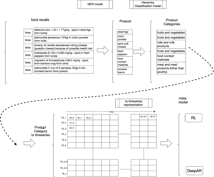
Schematic explanation of the data aspect to the end-to-end approach including the four main steps to the process

Regarding the second contribution of the proposed approach, i.e. food-recall forecasting, the proposed RL-based method was implemented yielding promising results compared to other well established approaches. The classified data from the NER task were represented in the time domain in order to incorporate RL in the prediction of food-recalls as a time-series use case. To this end, we defined a custom environment to express the "context" which our agent can interact with, a custom set of actions (A), which is specific to the time-series data and a reward $Ra(s, s ')$ function (1). The environment consists of a set of states (S) where each state is set to be an array of the last data points of the time-series. A shallow neural network was employed as the mechanism to select the appropriate action for the agent. The agent presented in this paper, is trained to predict the next value in a products’ time-series in terms of percentage change. To facilitate this, the actions available are a discrete set of numbers (20), drawn from statistical features of time-series (distribution, mean, median, min and max) that the agent can predict. A uniform experience replay mechanism is also employed to enable the agent to remember its past experiences and their corresponding rewards due to the nature of time-series forecasting problems.

4.2 Dataset

As mentioned earlier there is no open-source data for food recalls available. The utillized dataset has been provided by Agroknow as a real-world use case, composed of short text data that came from text mining of different online sources such as announcements, articles, and reports considering food recalls worldwide. It should be mentioned that the procedure of retrieving this data is out of the scope of this paper. The dataset in its final version was transformed in tabular format, consisting of the following information: ID, title (short text) and the product (label). Some indicative examples are depicted in Table 1.

Table 1 Initial short-texts with their corresponding products

Based on the data and the metadata of the web-crawlers that also include the timestamp of each recall, another dataset of 30 time-series was created, representing the daily number of food recalls of 30 implicated categories (such as ‘Food Additives and Flavorings’, ‘ Meat and products’, ‘Fish and products’ etc.) since 2000. Furthermore, Fig. 3a depicts some indicative categories of interest, while Fig. 3b presents the seasonality component of the examined time-series, highlighting that the majority of food recalls are being published on Fridays (considering days of week as time frame). Additionally, it is observed that during the summer months less food recalls occur compared to other months.

Fig. 3

a Food recalls of specific categories in time domain representation and b Average product recalls aggregated by month and day of the week. The x-axis represents a unit time (months or days) and the y-axis is measured in percentages

4.3 Preprocessing

Data in real-life cases are often noisy, high-dimensional, most of them may be broken or missing, so suitable preprocessing needs to be performed prior to any analytics task. As far as the NER task is considered, the preprocessing approaches aim to make the short texts, derived from heterogeneous sources, more readable and remove words and characteristics that may be assumed as noise. Even tough multiple preprocessing steps were considered our methodology consists of the following steps (a) Remove Numbers, (b) Remove specific words which as noise, (c) Lemmatization and lowercase, (d) Annotation. SpaCy framework which was used in this work for the NER provides an object describing what it considers to be an entity match. In this object, exists an “annotation” tuple which follows the form (starting character position, ending character position, type of entity). As an example we provide the tuple (13, 22, ’PRODUCT’), which corresponds to a product existing in the $13^{th}$ to $22^{nd}$ character of the given text. It is worth mentioning that not all texts contain an exact match and those cases are annotated as (0,0,”) providing the capability to our model to recognise the lack of an entity. For this reason, we split the data (during the train-test split) in such a way that both the training and the testing datasets contain examples with and without annotations. Table 2 summarises the transformations applied in each step providing a representative example.

Table 2 Preprocessing steps (vertical) for NER task

Table 3 Categories of time-series dataset

For the time-series forecasting task, the stationarity of the data was checked by using augmented Dickey-Fuller test (Cheung and Lai 1995). This process is of major importance for any predictive method that exploits historical data since these methods are usually based on the assumption that the data generation mechanism does not change over time. Furthermore, it should be noted that in terms of predictions, the prediction time-frames of the recalls may be 4 months, 6 months, or 12 months. Since the predictions will contribute to quality assurance and enable food safety professionals to ensure the continuity of their supply chain, minimize future risks and financial losses, we chose the smallest, i.e. a 4-month prediction window. Based on the latter, three options stand out:

• (i) Use the dataset as is, with its daily frequency resulting in a 120-time-step window of prediction. This is not recommended as most of the time-series produced are sparse leaving no obvious pattern to be learnt from.

• (ii) Resample the data in weeks, resulting in a 16-timestep window of prediction. While some patterns begin to emerge, the data in some cases are still very sparse and the cumulative error from the 16-step prediction is theoretically relatively big.

• (iii) Resample the data in months periods, providing stationary time-series with visible patterns and a lower theoretical accumulated error of prediction, since the window has been reduced to 4-timesteps.

Finally, another hypothesis to be tested was the forecasting task to be addressed as both univariate and multivariate assuming that complex non-linear feature interactions are present in our data when all the categories of food recalls are concerned. Consequently, taking also into consideration that 23 out of 30 in total time-series were stationary according to the Augmented Dickey-Fuller test that was conducted in the first place, and the fact that they differ greatly in statistical features (min, max, variance etc.) which would have a negative effect on some model’s performance while favor some others, the percentage change of the time-series was used instead. This enables the model to generalize better (arithmetic rate) while it also transforms remaining non-stationary time-series to stationary. Specifically, regarding the given data, to apply percentage change we had to deal with zero values. In most of the equivalent tasks handling those cases requires domain expertise as there is no "right" methodology. In our case one “recall” in every month in every category was added, which is insignificant and does not convey real change, to avoid having a zero in the percentage change denominator. Mathematically, let $x_t =\frac{(x_t+1)-(x_{t-1}+1)}{x_{t-1}+1}$ be the percentage change, $x_t$ is the number of recalls on month t.

4.4 Surrogate data

The original dataset size after preprocessing is $30*147$ and produced surrogate data matches its size, providing a combined dataset with of 30 * 247 data points. During our analysis, we refer to the corresponding data based on their ID number as cited in Table 3.

The most commonly used techniques for generating surrogate data for statistical analysis of nonlinear processes include random shuffling of the original time-series, Fourier-transformed surrogates, amplitude adjusted Fourier-transformed (AAFT surrogates), and iterated AAFT surrogates (IAAFT) (Dolan and Spano 2001). In our work we incorporated the IAAFT method to addresses the issue of power spectrum whitening, as the main drawback of AAFT method, by performing a series of iterations in which the power spectrum of an AAFT surrogate is adjusted back to that of the original data before the distribution is rescaled back to that of the original data.

4.5 Data models

4.5.1 NER task

Since our goal is to classify short food recall text based on implicated product (discarding possible noisy patterns), and since there is no any open-source pre-trained model specified for food product recognition to directly apply transfer learning for NER task, we approached the problem by training from scratch a Deep Neural Network utilizing the spaCy framework (Honnibal and Montani 2017). The training took under consideration the custom made PRODUCT annotations. The central data structures in spaCy are the Doc and the Vocab. The Doc object owns the sequence of tokens and all their annotations. Finally, regarding our problem setup an architecture of Residual CNN (ResNET) (He et al. 2016) network yields the best results in terms of the evaluation metrics that will be analysed in detail in the next subsection. In traditional neural networks, each layer feeds into the next layer. In a network with residual blocks, each layer feeds into the next layer and directly into the layers about 2-3 hops away.

In the computer vision domain, CNNs are used for dimensionality reduction or reducing matrices to vectors with the usage of multiple filters focusing in setting the stride, kernel size, padding etc. In SpaCy the CNNs are used in a way similar to what is described in (Collobert et al. 2011) but of course leveraging the up-to-date implementation details to facilitate training and accuracy. The founding block of the CNNs used by SpaCy are the trigramcnn that concatenates the embeddings of each word with those of its two neighboring words. For example, if the embedding dimension of each word was 128-dimensions this concatenation would create a 384-dimension vector representing those three words. After this, an MLP is used to reduce this input’s representation dimension back to the original, relearning the meaning of each word based on its context. While staking these layers together a sort of ”effective receptive field” in terms of vision emerges. This happens due to staking, thus making the vectors’ representations sensitive to information found in words further away from the initial term. Another aspect of interest, is the usage of residual connections from layer to layer. The latter means that the output of each layer is the output produced by the layer plus its input facilitating training. This has a fundamental effect as it implies that the output space vector of each convolutional layer is likely to be similar to the output space of the input vector—due to using and feeding forward the input feature at each layer.

4.5.2 Forecasting task

Regarding the time-series forecasting approach, several models have been utilized, as summarized below:

• A DeepAR Estimator,which implements an (Recurrent Neural Network) RNN-based model, close to the one described in Salinas et al. (2019). More specifically it applies a methodology for producing accurate probabilistic forecasts, based on training an autoregressive recurrent neural network model on many related time-series. Recurrent Neural Net- work is a feed-forward neural network that has an internal memory. The “recurrence” explains the fact that the produced output is copied and sent back into the recurrent network as an additional input. For making a decision regarding every output of every layer, it considers the current input and the output that it has learned from the previous input. That capability makes them perfect candidate for handling sequence data

• A Simple Feed Forward Estimator which implements a simple Multi-layer Perceptrons (MLP) model predicting the next target time-steps given the previous ones. MLP is a supervised learning algorithm that learns a function by training on a dataset, where n is the number of dimensions for input and o is the number of dimensions for output. Given a set of features $X= {x1,x2,...,xn}$ and a target y, it can learn a non-linear function of approximation for either classification or regression.Implemented as described (Pedregosa et al. 2011).

• One Deep Factor Estimator, an implementation of Wang et al. (2019). It uses a global RNN model to learn patterns across multiple related time-series and an arbitrary local model to model the time-series on a per time-series basis.

• A Seasonal Naive Estimator, based on data seasonality. This model predicts $Y(T+k)=y(T+k-h)$ where T is the forecast time, $k \epsilon [0, prediction length -1]$ and h = season length. If a time-series is shorter than season length, then the mean observed value is used as prediction.

• A WaveNet Estimator based on WaveNet architecture (Oord et al. 2016) was used. WaveNet, is a deep neural network created for generating raw audio waveforms. The model is fully probabilistic and auto-regressive, with the predictive distribution for each audio sample conditioned on all previous ones, yielding state of the art results in tasks such as text-to speech conversions, source disaggregation etc.

On top of the implementation and experimentation of the aforementioned models, an Reinforcement Learning approach was researched and developed, including both a custom environment for time-series and an agent. This custom environment could also be utilized in other time-series cases apart from food-recalls forecasting. The RL agent interacts with this environment in discrete time steps. At each time t, the agent receives an observation $O_t$, which typically includes the reward $R_t$ and the state $S_t$. In this custom environment the states from the historical values and the rewards are produced by applying the reward function 1. The Agent then chooses an action from the set of available actions $A_t$, which is subsequently sent to the environment. The environment moves to a new state and the reward associated with the transition $(S_t,A_t,S_{t+1})$ is determined.

The design of the reward function depends on the actions we want the agent to favor. In this work, the reward Rt at time t is:

$$\begin{aligned} R_t = 1/log(MSE(Y_t,\hat{Y_t}))+k \end{aligned}$$

(1)

where $Y_{t}$ is the actual number of recalls for the given time-step, $\hat{Y}_{t}$ is the predicted one and k is a small positive integer.

With Q-learning the agent seeks to learn a policy that maximizes the total reward for the selected set of actions in a given environment. In practice, a Q-table is a [state, action] table where the values of each action are stored. A DQN architecture with experience replay was realized as described below:

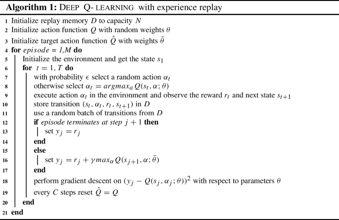
Where $\gamma$ is the discount factor, used to balance the importance of future and immediate reward, $\alpha$ (learning rate) defines the rate in which the newly calculated value of Q affects the old one. It should be highlighted that the algorithm provides very good results in the cases of small action and state spaces. In the cases of prohibitive size $S_t,A_t$ a neural network is proposed to approximate and compress the Q-table, where updating the weights w corresponds to updating the Q-values. One improvement of Deep Q-learning algorithm has been achieved by using an additional neural network with the same architecture but with fixed weights $\hat{w}$ that are updated every n iterations to break the correlation between updated values w and $\Delta _w$.

5 Results

In this section we initially provide a brief description of the evaluation strategy regarding the approaches introduced in this paper: the NER task for classification, and the time-series forecasting for food recalls prediction. Then the results of each approach are presented respectively.

5.1 NER task

Precision, Recall and F1-score at a token level are the most common evaluation metrics for NER tasks (Batista 2018). However in the examined use-case, it is more useful to evaluate at a full named-entity level. There are some metrics that are appropriate for this approach as they are measuring the full named-entity token performance presented (Sundheim and Chinchor 1993) . Following this strategy the metrics can be defined in terms of comparing the response of a system against the golden annotation as follows:

• Correct (COR): both are the same,

• Incorrect (INC): the output of a system and the golden annotation don’t match,

• Partial (PAR): system and the golden annotation are somewhat “similar” but not the same,

• Missing (MIS): a golden annotation is not captured by a system,

• Spurius (SPU): system produces a response which doesn’t exist in the golden annotation,

In order to cover the scenarios defined in our problem, we need to consider the differences between NER output and golden annotations based on two axes, the surface string, and the entity type. Another equivalent approach was presented in International Workshop on Semantic Evaluation (SemEval 13) (Segura Bedmar et al. 2013), where introduced four ways to measure precision/recall/f1-score results based on the metrics defined by MUC

• Strict: exact boundary surface string match and entity type;

• Exact: exact boundary match over the surface string, regardless of the type;

• Partial: partial boundary match over the surface string, regardless of the type;

• Type: some overlap between the system tagged entity and the gold annotation is required;

Furthermore, to define precision/recall/f1-score two more variables need to be calculated:

The number of gold-standard annotations contributing to the final score given as:

$$\begin{aligned} POSSIBLE(POS) = COR + INC + PAR + MIS = TP + FN \end{aligned}$$

(2)

And the number of annotations produced by the NER system:

$$\begin{aligned} ACTUAL(ACT) = COR + INC + PAR + SPU = TP + FP \end{aligned}$$

(3)

In brief precision is the percentage of correct named-entities found by the NER system, and recall is the percentage of the named-entities in the golden annotations that are retrieved by the NER system. These are calculated either for exact match (i.e., strict and exact ) or for partial match (i.e., partial and type) scenario by the following equations:

Exact Match (i.e., strict and exact)

$$\begin{aligned}&Precision = \frac{COR}{ACT} = \frac{TP}{TP+FP} \end{aligned}$$

(4)

$$\begin{aligned}&Recall = \frac{COR}{POS} = \frac{TP}{TP+FN} \end{aligned}$$

(5)

Partial Match (i.e., partial and type)

$$\begin{aligned}&Precision = \frac{COR\ +\ 0.5\ \times \ PAR}{ACT} = \frac{TP}{TP+FP} \end{aligned}$$

(6)

$$\begin{aligned}&Recall = \frac{COR\ +\ 0.5\ \times \ PAR}{POS} = \frac{COR}{ACT} = \frac{TP}{TP+FP} \end{aligned}$$

(7)

Table 4 presents some examples from the utilized dataset, explaining how can be evaluated based on these the above-mentioned metrics. Then precision/recall/f1-score are calculated for each different evaluation schema applied on a 4-fold stratified scheme of evaluating our results and the average results in terms of the evaluation strategy are presented in Table 5.

Table 4 Evaluation Scheme based on Semantic Evaluation (SemEval 13)

Table 5 Results in terms of evaluation metrics

5.2 Time-series forecasting

The total training data consist of a matrix $N \in \mathbb {R}^{30 \times 147}$, where ‘30’ corresponds to the number of time-series of products and ‘147’ to the last 147 month time-steps of each. In order to obtain more reliable results, we trained every model 47 times on a rolling window of 100 time-steps forming 47 tables $\in \mathbb {R}^{30x100}$ (ex. [30,1-100], [30,2-101] etc.). While all models share some hyper-parameters such as $epochs \leftarrow 200$, the $length(prediction) \leftarrow 4$ and $length(context) \leftarrow 12$ months, some others are specific only to some models. These specific parameters were fine-tuned using grid-search techniques, as a fundamental step of the ML pipeline. Grid-search and Random-search algorithms are widely used for hyperparameter tuning. Basically, the domain of the hyperparameters into a discrete grid. Then, every combination of values of this grid (i.e. grid-search) is used in terms of using cross-validation. The point of the grid that maximizes the average value in cross-validation, is the optimal set of values for the hyperparameters.

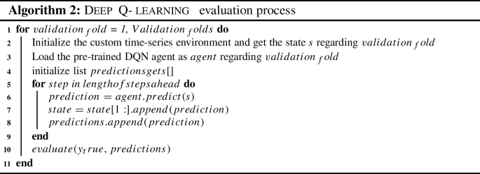
In common ML usage, cross-validation methods reflect a pitfall in a time-series forecasting approach, as they may result in a significant overlap between train and test data. Thus, the optimum approach is to simulate models in a ‘walk-forward’ sequence, periodically re-training the model to incorporate specific chunks of data available at that point in time. This procedure is depicted in Fig. 4 while regarding the validations process followed in the case of the RL model, Algorithm 2 has been applied.

Fig. 4

Proposed one step forward validation scheme

Based on the evaluation, we observed the following results in terms of the Mean Squared Error (MSE) with the usage of the original data, the data after applying the preprocessing mentioned in the corresponding section and with the enriched dataset using surrogate data. The results are presented in Table 6. Furthermore, the relevant plots are depicted in Fig. 5, showing the estimators on specific time-series.

Fig. 5

Indicative examples predictions using Deep AR estimator on specific time-series. Marked in dark green is the 0.5 prediction (confidence) interval and marked in light green is the 0.9 prediction (confidence) interval. The x-axis presents time in moths while the y-axis represents percentage change of recalls per month. The prediction horizon is 4 months. While the blue line represent the actual values of the time-series

Tables 6 and 7 are divided into three parts where the comparison of the models in different cases is depicted. The first part uses univariate data (predictions are based solely on one time-series at a time), while the second utilizes the surrogate data in Table 6 and multivariate data (all 30 time-series are used for predictions) in Table 6 and multivariate data (all 30 time-series are used for predictions) in Table 7. The last part of both tables provide a comparison with the proposed RL approach.

The Deep Factor model is omitted in the univariate case as it is not applicable due to the existence of a global RNN model as described in Wang et al. (2019), used to learn patterns across multiple related time-series.

The results presented in Tables 6 and 7 which can be found in Appendix A, highlight that the model with the best performance in most cases is the Deep AR model, while the WaveNet follows up due to its capability of capturing long term dependencies like LSTMs but with less training. The Simple Feed Forward network wins in 4/30 time-series in the multivariate setup.

As expected, even though the seasonal model achieves mostly low errors due to the way of predicting values it never outperforms all deep models. Another interesting result is that utilizing univariate models seems to be more accurate. This contradicts our initial hypothesis that by using multivariate data streams, complex non-linear feature interactions will emerge, facilitating the optimization of the models. As mentioned above the data were normalized in case of different scales. The inferiority of the multivariate dataset arises from the fact that a wide but not deep set of data is exploited, making it harder to distinguish between signal and noise as well as from the lack of correlation between time-series.

Additionally, we can express guarded optimism for the usage of analogous/surrogate data as an enrichment technique, which can be further explored, since results presented in Table 6, demonstrate a successful trial of the proposed approach in some cases.

Finally, the RL model that utilized our custom environment yields promising results. According to Table 6, it outperforms all other models in 9/30 datasets. Taking under consideration the fact that the RL model was trained on univariate time-series without surrogate data we can reinforce the belief that using univariate data is appropriate for this task.

In a real-world scenario as the case presented in this paper, there are other features than accuracy of the results that may make a model more suitable. Such features, are for example the required computing and data resources and the model’s complexity. This paper also introduces an approach to optimise the process of time-series forecasting by accounting for the aforementioned features. The latter is achieved by a meta-model, which proposes the best-fit model to be used without exhaustively trying and evaluating all of the possible candidate-models. Towards this direction, this model selection should be based on some indicative statistical metrics of each time-series such as Augmented Dickey-Fuller (ADF) denoting the stationarity, standard deviation (SD), block entropy and hjorth-mobility. As seasonal component, we have used the results of univariate Seasonal model of GlounTS. Additionally, Table 8 of the appendix presents the values for the aforementioned statistical metrics for each time-series. Focusing on the approaches that yield the best results (univariate DeepAR and RL) we calculated the correlation between the prediction error and the various statistical metrics, presenting them in the heat-map of Fig. 6.

Fig. 6

Correlations of the univariate Deep Ar and RL models regarding statistical metrics

Also in Table 8 are presented the values for the aforementioned statistical metrics for each time-series to supplement the reader with useful information.

It is obvious that the RL model is highly positively correlated with SD and hjorth-mobility. The latter means that when a time-series has bigger value of SD, the expectation of the error for the RL model follows the same trend. The reason for that is that we used a static action-space for the RL model.Given our dataset, and results of the models, we applied a tree model in an attempt to explain the decisions made for model selection. The results are depicted in Fig. 7.

Fig. 7

Decision Tree for model selection, red color denotes the selection of DeepAR model, while with the blue color the RL model

Specifically, in this figure red color nodes denote the selection of DeepAR model, and the blue ones the RL model. The main findings of the implementation of the meta-model can be summarised in the following statements. When the hjorth mobility is high we can confidently use the DeepAR model, which means that the models are better at capturing different kinds of variation of the time-series. Besides that, another important factor is the block entropy which is an estimation of the entropy growth curve with respect to a window size. From the tree we see that when the hjorth mobility is big we use with confidence the Deep AR model which means that this model is better at capturing the intra-block variation of the time-series. On the other hand, when we observe extreme values of block entropy we tend to choose the RL model which means that it can better capture the inter-block variation. The exploitation of such a model enables the utility of the two best models in a hybrid way, optimising the predicting outcomes in terms of accuracy by selecting the best model for each time-series category.

The exploitation of such a model enables the utilization of the two best-fit models in a hybrid way, optimising the predicting outcomes in terms of accuracy by selecting the best-fit model for each time-series category.

6 Conclusions

The approaches presented in this paper have been implemented as a framework to address one of the main challenges in the food safety sector, which is the constant optimization of the monitoring, early detecting and predicting the food recall trends. The present research realizes an overall optimisation both in terms of performance, as the meta-model and the usage of surrogate data enhance the predicted outcomes of the proposed forecasting model, and in terms of adaptability and continuous optimization by applying a RL model for time-series prediction. One major obstacle to apply the proposed approaches in large scale is the adaptability to new types of resources. This is addressed within the context of our research by introducing an RL-based prediction approach offering continuous optimization through specific training intervals for the NER model.

With regards to time-series forecasting, we presented specific approaches in the field of time-series forecasting, while addressing key challenges that include interpretation, scale, accuracy and complexity (which are inherent in many cases of time-series manipulation). Though the experimentation and evaluation, we compared a variety of approaches based on deep neural networks and statistical terms. The complementary model, which consists of an RL (DQN) model, provides promising results in terms of food recalls prediction.

Regarding the future work, the two aforementioned improvements represent key areas of future work that will be generally beneficial for monitoring dynamic and complex recall announcements published on different sources. We also plan to continue to refine our approaches by applying continuous action space RL model, utilizing a multivariate and multi-step actions environment and try leveraging an approach close to Signal2Vec. A Time-series Embedding Representation used for dimensionality reduction for time-series (Nalmpantis and Vrakas 2019). Moreover, it is within our future plans to address the case of large number of ‘spurious’ labeled data. This is tackled by the approaches such as Karamanolakis et al. (2020), which consists an extension of OpenTag for multiple product categories called TXtract. Specifically, specific entity (’annotation’) for each product category will be assigned instead of a universal ”PRODUCT” entity. This is expected to improve or at least enhance the downstream task transforming the unstructured text data to time-series. On this note, we plan to develop a supervised learning scenario encoding the lexical semantics of the recall announcement with embeddings to predict the product category listed in the recall. Additionally, we are currently experimenting with fine-tuning a BERT model with the usage of HuggingFace interface to compare or even improve our initial NER performance. Finally, making the proposed NER model multilingual is another highly rated production-based requirement.

Results

See Tables 6, 7 and 8.

Table 6 Comparison between univariate approach, data augmentation and Reinforcement Learning

Table 7 Comparison between univariate, multivariate and Reinforcement Learning approach

Table 8 Hjorth mobility, block entropy, ADF, Variance and Seasonality component of the time-series

References

Alexandrov, A., Benidis, K., Bohlke-Schneider, M., Flunkert, V., Gasthaus, J., Januschowski, T., Maddix, D.C., Rangapuram, S., Salinas, D., & Schulz, J., et al. (2019) Gluonts: Probabilistic time series models in python. arXiv:1906.05264
Batista, D.S. (2018). Named-entity evaluation metrics based on entity-level. https://www.davidsbatista.net/blog/2018/05/09/Named_Entity_Evaluation/.
Beltagy, I., Lo, K., & Cohan, A. (2019). Scibert: A pretrained language model for scientific text. arXiv:1903.10676
Bengio, Y., Lamblin, P., Popovici, D., & Larochelle, H. (2007). Greedy layer-wise training of deep networks. In Advances in neural information processing systems (pp. 153–160).
Calabuig, J., Falciani, H., & Sánchez-Pérez, E. (2020) Dreaming machine learning: Lipschitz extensions for reinforcement learning on financial markets. Neurocomputing
Cheung, Y. W., & Lai, K. S. (1995). Lag order and critical values of the augmented dickey-fuller test. Journal of Business & Economic Statistics, 13(3), 277–280.
Collobert, R., Weston, J., Bottou, L., Karlen, M., Kavukcuoglu, K., & Kuksa, P. (2011). Natural language processing (almost) from scratch. Journal of Machine Learning Research, 12(ARTICLE), 2493–2537.
Devlin, J., Chang, M.W., Lee, K., & Toutanova, K. (2018) Bert: Pre-training of deep bidirectional transformers for language understanding. arXiv:1810.04805
Dolan, K. T., & Spano, M. L. (2001). Surrogate for nonlinear time series analysis. Physical Review E, 64(4), 046128.
Fong, S.J., Li, G., Dey, N., Crespo, R.G., & Herrera-Viedma, E. (2020) Finding an accurate early forecasting model from small dataset: A case of 2019-ncov novel coronavirus outbreak. arXiv:2003.10776
Fu, T. C. (2011). A review on time series data mining. Engineering Applications of Artificial Intelligence, 24(1), 164–181.
Gendel, S. M., & Zhu, J. (2013). Analysis of us food and drug administration food allergen recalls after implementation of the food allergen labeling and consumer protection act. Journal of Food Protection, 76(11), 1933–1938.
Hammerton, J. (2003). Named entity recognition with long short-term memory. In Proceedings of the seventh conference on Natural language learning at HLT-NAACL 2003 (pp. 172–175)
He, K., Zhang, X., Ren, S., & Sun, J. (2016). Deep residual learning for image recognition. In Proceedings of the IEEE conference on computer vision and pattern recognition (pp. 770–778).
Hessel, M., Modayil, J., Van Hasselt, H., Schaul, T., Ostrovski, G., Dabney, W., Horgan, D., Piot, B., Azar, M., & Silver, D. (2018). Rainbow: Combining improvements in deep reinforcement learning. In Thirty-Second AAAI conference on artificial intelligence
Honnibal, M., & Montani, I. (2017). spaCy 2: Natural language understanding with Bloom embeddings, convolutional neural networks and incremental parsing. To appear
Karamanolakis, G., Ma, J., & Dong, X.L. (2020). TXtract: Taxonomy-aware knowledge extraction for thousands of product categories. In: Proceedings of the 58th Annual Meeting of the Association for Computational Linguistics, pp. 8489–8502. Association for Computational Linguistics, Online. https://doi.org/10.18653/v1/2020.acl-main.751. https://aclanthology.org/2020.acl-main.751
Lai, G., Chang, W.C., Yang, Y., & Liu, H. (2018). Modeling long-and short-term temporal patterns with deep neural networks. In The 41st international ACM SIGIR conference on research & development in information retrieval (pp. 95–104).
Lebret, R., & Collobert, R. (2013) Word emdeddings through hellinger pca. arXiv:1312.5542
Li, J., Sun, A., Han, J., & Li, C. (2020). A survey on deep learning for named entity recognition. IEEE Transactions on Knowledge and Data Engineering
Luo, F., Fang, P., Qiu, Q., & Xiao, H. (2021). Features induction for product named entity recognition with CRFS. In Proceedings of the 2012 IEEE 16th International Conference on Computer Supported Cooperative Work in Design (CSCWD) (pp. 491–496). IEEE
Maharana, A., Cai, K., Hellerstein, J., Hswen, Y., Munsell, M., Staneva, V., et al. (2019). Detecting reports of unsafe foods in consumer product reviews. JAMIA Open, 2(3), 330–338.
Makridis, G., Mavrepis, P., Kyriazis, D., Polychronou, I., & Kaloudis, S. (2020). Enhanced food safety through deep learning for food recalls prediction. In International conference on discovery science, Springer (pp. 566–580).
Marvin, H. J., Janssen, E. M., Bouzembrak, Y., Hendriksen, P. J., & Staats, M. (2017). Big data in food safety: An overview. Critical Reviews in Food Science and Nutrition, 57(11), 2286–2295.
Mikolov, T., Chen, K., Corrado, G., & Dean, J. (2013). Efficient estimation of word representations in vector space. arXiv:1301.3781
Mikolov, T., Sutskever, I., Chen, K., Corrado, G.S., & Dean, J. (2013). Distributed representations of words and phrases and their compositionality. In Advances in neural information processing systems (pp. 3111–3119).
Nalmpantis, C., & Vrakas, D. (2019). Signal2vec: Time series embedding representation. In International conference on engineering applications of neural networks, Springer (pp. 80–90).
Nyachuba, D. G. (2010). Foodborne illness: Is it on the rise? Nutrition Reviews, 68(5), 257–269.
Oord, A.v.d., Dieleman, S., Zen, H., Simonyan, K., Vinyals, O., Graves, A., Kalchbrenner, N., Senior, A., & Kavukcuoglu, K. (2016). Wavenet: A generative model for raw audio. arXiv:1609.03499
Parmezan, A. R. S., Souza, V. M., & Batista, G. E. (2019). Evaluation of statistical and machine learning models for time series prediction: Identifying the state-of-the-art and the best conditions for the use of each model. Information Sciences, 484, 302–337.
Pedregosa, F., Varoquaux, G., Gramfort, A., Michel, V., Thirion, B., Grisel, O., et al. (2011). Scikit-learn: Machine learning in Python. Journal of Machine Learning Research, 12, 2825–2830.
Pennington, J., Socher, R., & Manning, C.D. (2014). Glove: Global vectors for word representation. In Proceedings of the 2014 conference on empirical methods in natural language processing (EMNLP) (pp. 1532–1543).
Pfeiffer, J., Simpson, E., & Gurevych, I. (2020). Low resource multi-task sequence tagging–revisiting dynamic conditional random fields. arXiv:2005.00250.
Popovski, G., Kochev, S., Seljak, B.K., & Eftimov, T. (2019). Foodie: a rule-based named-entity recognition method for food information extraction. In Proceedings of the 8th international conference on pattern recognition applications and methods (pp. 915–922).
Popovski, G., Seljak, B. K., & Eftimov, T. (2020). A survey of named-entity recognition methods for food information extraction. IEEE Access, 8, 31586–31594.
Salinas, D., Flunkert, V., Gasthaus, J., & Januschowski, T. (2019). Deepar: Probabilistic forecasting with autoregressive recurrent networks. International Journal of Forecasting
Segura Bedmar, I., Martinez, P., & Herrero Zazo, M. (2013). Semeval-2013 task 9: Extraction of drug-drug interactions from biomedical texts (ddiextraction 2013). Association for Computational Linguistics
Sherstov, A.A., & Stone, P. (2005). Function approximation via tile coding: Automating parameter choice. In International symposium on abstraction, reformulation, and approximation, Springer (pp. 194–205).
Socher, R., Huval, B., Manning, C.D., & Ng, A.Y. (2012). Semantic compositionality through recursive matrix-vector spaces. In Proceedings of the 2012 joint conference on empirical methods in natural language processing and computational natural language learning, (pp. 1201–1211).
Socher, R., Manning, C.D., & Ng, A.Y. (2010). Learning continuous phrase representations and syntactic parsing with recursive neural networks. In Proceedings of the NIPS-2010 deep learning and unsupervised feature learning workshop, vol. 2010, pp. 1–9
Strubell, E., Verga, P., Belanger, D., & McCallum, A. (2017). Fast and accurate entity recognition with iterated dilated convolutions. arXiv:1702.02098.
Sundheim, B.M., & Chinchor, N. (1993). Survey of the message understanding conferences. In HUMAN LANGUAGE TECHNOLOGY: Proceedings of a Workshop Held at Plainsboro, New Jersey, March 21-24, 1993
Sutton, R. S., Barto, A. G., et al. (1998). Introduction to reinforcement learning (Vol. 135). Cambridge: MIT Press.
Tsuboi, Y. (2014). Neural networks leverage corpus-wide information for part-of-speech tagging. In Proceedings of the 2014 conference on empirical methods in natural language processing (EMNLP), (pp. 938–950).
Wang, Y., Smola, A., Maddix, D.C., Gasthaus, J., Foster, D., & Januschowski, T. (2019). Deep factors for forecasting. arXiv:1905.12417
Yom-Tov, E. (2017). Predicting drug recalls from internet search engine queries. IEEE journal of Translational Engineering in Health and Medicine, 5, 1–6.
Zhang, Z., Zohren, S., & Roberts, S. (2020). Deep reinforcement learning for trading. The Journal of Financial Data Science, 2(2), 25–40.
Zhao, J., & Liu, F. (2008). Product named entity recognition in Chinese text. Language Resources and Evaluation, 42(2), 197–217.
Zheng, G., Mukherjee, S., Dong, X.L., & Li, F. (2018). Opentag: Open attribute value extraction from product profiles. In Proceedings of the 24th ACM SIGKDD international conference on knowledge discovery & data mining, (pp. 1049–1058).
Zhong, Z., & Chen, D. (2020). A frustratingly easy approach for entity and relation extraction. arXiv:2010.12812.
Acknowledgements
The research leading to the results presented in this paper has received funding from the European Union’s Project CYBELE under grant agreement no 825355.
Funding
The authors declare that, the research leading to the results presented in this paper has received funding from the European Union’s Project CYBELE under grant agreement no 825355.
Author information
Authors and Affiliations
Contributions
Not Applicable
Corresponding author
Ethics declarations
Conflicts of interest
The authors declare that they have no known competing financial interests or personal relationships that could have appeared to influence the work reported in this paper.
Ethics approval
Consent to participate
Consent for publication
Code availability
A Git repository containing all the code for this project is created that can be found at this link Github Repository.
Additional information
Communicated by Editors: Annalisa Appice, Grigorios Tsoumakas.
Publisher's Note
Springer Nature remains neutral with regard to jurisdictional claims in published maps and institutional affiliations.
Results
Rights and permissions
About this article
Cite this article
Makridis, G., Mavrepis, P. & Kyriazis, D. A deep learning approach using natural language processing and time-series forecasting towards enhanced food safety. Mach Learn 112, 1287–1313 (2023). https://doi.org/10.1007/s10994-022-06151-6
Received:
Revised:
Accepted:
Published:
Issue Date:
DOI: https://doi.org/10.1007/s10994-022-06151-6