Abstract
Reduced-order models (ROMs) become increasingly popular in industrial design and optimization processes, since they allow to approximate expensive high fidelity computational fluid dynamics (CFD) simulations in near real-time. The quality of ROM predictions highly depends on the placement samples in the spanned parameter space. Adaptive sampling strategies allow to identify regions of interest, which feature e.g. nonlinear responses with respect to the parameters, and therefore enable the sensible placement of new samples. By introducing more samples in these regions, the ROM prediction accuracy should increase. In this contribution we investigate different adaptive sampling strategies based on cross-validation, Gaussian mean-squared error, two methods exploiting the CFD residual and a two manifold embedding methods. The performance of those strategies is evaluated and measured by their ability to successfully identify the regions of interest and the resulting sample placement in terms of different quantitative statistical values. We further discuss the reduction of the ROM prediction error over the adaptive sampling iterations and show that depending on the adaptive sampling strategy, the number of required samples can be reduced by 35–44% without deteriorating model quality compared to a Halton sequence sampling plan.
1 Introduction
In today’s industrial applications such as optimization, interactive design or aero-loads, a large number of high fidelity simulations are required in order to improve or analyze the engineering problems at hand. Varying number of flow conditions and geometric parameters make it infeasible to compute all high-fidelity solutions of the entire flight envelope for the compressible Navier–Stokes equations with computational fluid dynamics (CFD). Especially in the industrial context, reduced-order models (ROMs) can be used to generate the required data and decrease the actual number of computed solutions necessary [1].
However, the approximation of the solution manifold and hence the quality of data-driven ROMs, i.e., the algorithmic efficiency and numerical accuracy, strongly depends on the number of sampled parameters and their location in the parameter space. Since the to be modeled processes often are non-linear with respect to the parameters it is intuitively obvious that the higher the dimension of the parameter space, the more snapshots are needed to build an accurate ROM.: “if a certain level of prediction accuracy is achieved by sampling a one-variable space in n locations, to achieve the same sample density in a k-dimensional space, \(n^{k}\) observations are required” [2, Section 1.1]. The latter fact is often referred to as the curse of dimensionality. The main goal is to keep the number of calculations of full-order snapshots small and at the same time the prediction quality of the resulting ROM high. Therefore, a single sample needs represent the dynamics of flow and introduce as much information into the model as possible. In order to find the locations of these high information samples in the parameter space an efficient sampling strategy needs to be devised.
In [3] the sampling strategies are divided into one-shot, sequential space-filling and sequential adaptive strategies. A significant advantage of one-shot strategies is the possibility to compute all samples for the ROM in parallel if the required resources are available. Prominent one-shot methods are the Full Factorial Design, Latin Hypercube Sampling [4, 5] and the Halton Sequence [6]. In contrast, sequential adaptive strategies focus on detecting the best possible sample location and iteratively add more samples to the parameter domain. Each new sample location in the parameter space is determined by an objective function and all previously compute samples. With this strategy an optimal placement for a fixed number of samples in the parameter domain compared to the one-shot strategies can be achieved resulting in a higher ROM prediction quality. Possible sequential adaptive strategies are variance [7], query-by-committee [8], cross-validation [9] or gradient based [3, 10].
In the last decade, ROMs are more and more used in industry. A standard Reynolds-averaged Navier–Stokes (RANS) CFD simulation in the automobile industry has a computational time of 12 h on 1000 cores. Driven by budget, the computation of high-fidelity CFD simulations is limited. Often a combination of one-shot and adaptive sampling strategies is applied to obtain the best mix of quick turn around timings and good ROM predictions.
Most of the contributions with respect to adaptive strategies focus on surrogates and only very few on improving the prediction quality of ROMs. In this contribution, sequential adaptive strategies for ROMs based on cross-validation, CFD flow residuals and space embedding using isomap are developed and compared against a Gaussian based sequential space-filling strategy and the one-shot Halton strategy. The performance of the sampling strategies is analyzed with the evaluation of different error norms for the resulting ROMs. In addition, the potential to reduce the computational effort by employing adaptive over one-shot strategies is investigated.
Organization: Section 2 describes the governing equations of fluid dynamics. Sections 3 and 4 provide an overview of the ROMs and adaptive sampling strategies used in this paper respectively. The two test cases used are covered in Sect. 5 followed by the results in Sect. 6.
2 Governing equations
Consider the governing equations of fluid dynamics [11], more precisely the Euler, Navier–Stokes and Reynolds-averaged Navier–Stokes (RANS) equations, in a generalized notation. As also shown in [12] the underlying partial differential equations (PDEs) are spatially discretized on a grid of size \(n_{g}\) for some aerodynamic configuration. The mean-flow variables are made up of density, \(\rho\), the velocity components \(u_{x}\), \(u_{y}\) and \(u_{z}\), the total energy, E, as well as the variables associated with the turbulence model. The number of these variables is denoted with \(n_{v}\). The total length of the discretized flow solution vector is then given by \(n=n_{g}n_{v}\). With a given finite volume scheme the corresponding system of semi-discrete ordinary differential equations can be written as
where \(t\in {\mathbb {R}}^{+}\) denotes the time, \(p\in {\mathbb {R}}^{d}\) is the vector of input parameters, \(\mathbf {W}\left( t;\,\,\mathbf {p}\right) \in {\mathbb {R}}^{n}\) is the state vector of primitive variables and \(\mathbf{res}\left( \mathbf {W}(t;\mathbf {p})\right) \in {\mathbb {R}}^{n}\) is the vector of flux residuals corresponding to the state solution \(\mathbf {W}(t;\,\,\mathbf {p})\).
The diagonal matrix \(\Omega \in {\mathbb {R}}^{n\times n}\) with \(n_{v}\) sub-blocks, each containing the cell volumes \(\mathrm{vol}_{1},\ldots ,\mathrm{vol}_{n_{g}}\) of the corresponding computational grid on the diagonal, stems from the spatial discretization of the flow problem and induces the discrete \(L_{2}\)-metric.
If the CFD flux residual vanishes or the time derivative drops out in Eq. (1), steady state is achieved.
In the current works the ROM methods are applied to the flow state vectors. However, ROMs can also be used with conservative variables or even different governing PDE problems.
3 Reduced-order modelling
3.1 Proper orthogonal decomposition with interpolation
In the context of CFD simulations, PODs are widely used to model the distributed flow field variables of 2- or 3-dimensional problems. A common approach to computing a POD-based ROM is using the method of snapshots. With it, the POD basis is derived by solving the eigenvalue problem of the snapshots correlation matrix (also see [13]). For m CFD steady state snapshots \(\mathbf {W}^{i}=\mathbf {W}(\mathbf {p}^{i})\in \mathbb {R}^{n}\) with \(i=1,\ldots ,m\) and each snapshot depending on a unique set of parameters \(\mathbf {p}^{i}=\left( p_{1}^{i},\ldots ,p_{d}^{i}\right) \in \mathbb {R}^{d}\) the snapshot matrix is defined by
With the correlation matrix \(W^{T}W\in {\mathbb {R}}^{m\times m}\) the normalized eigenvectors \(\mathbf {V}^{j}\in \mathbb {R}^{m}\) and corresponding eigenvalues \(\lambda _{j}\) are computed by solving the eigenvalue problem
The m orthonormal POD modes \(\mathbf {U}^{j}\) are then given with
The initial snapshots \(\mathbf {W}^{i}\) can be expressed with the newly found basis
where the coefficients a are determined with
Analogous to Eq. (6) an approximate flow solution \(\mathbf {W}^{*}\) at an untried parameter combination \(\mathbf {p}^{*}\) can be computed by a coefficient vector \(\mathbf {a}^{*}=\left( a_{1},\ldots ,a_{m}\right) \in \mathbb {R}^{m}\) as follows:
[14] shows, that the coefficient vector \(\mathbf {a}^{*}\) can be obtained by interpolating its components at the parameter combination \(\mathbf {p}^{*}\) based on the data set \(\left\{ (\mathbf {p}^{i},\mathbf {a}^{i})\right\} _{i=1}^{m}\). This method will be referred to as POD+I.
Further reviews on POD-based ROMs can be found in [15, 16]. Also, [17, 18] as well as references therein give a comprehensive introduction into the topic.
3.2 Isomap with interpolation
Similar to POD+I, isomap can be used to model the 2- or 3-dimensional distributed flow field variables of a CFD simulation. It is a ROM based on manifold learning (ML) [19, 20] can be constructed. ML methods try to recover, in a meaningful way, low-dimensional structures hidden in high-dimensional data, which is assumed to lie on or close to a smooth embedded submanifold \({\mathcal {W}}\subset {\mathbb {R}}^{n}\). One of the most popular ML methods, namely Isomap [21], is used here to extract low-dimensional structures hidden in a given high-dimensional data set given by \(W:=\{\mathbf {W}^{1},\ldots ,\mathbf {W}^{m}\}\subset {\mathbb {R}}^{n}\), where \(\mathbf {W}^{i}=\mathbf {W}(\mathbf {p}^{i})\) depends on the parameter combination \(\mathbf {p}^{i}\in \mathcal {P}\), \(i=1,\ldots ,m\). Exploiting the theory of Riemannian geometry [22, 23], Isomap approximates the geodesic distances between each pair of data vectors \(\mathbf {W}^{i}\) and \(\mathbf {W}^{j}\) and constructs an embedding of corresponding low-dimensional vectors \(Y=\{\mathbf {y}^{1},\dots ,\mathbf {y}^{m}\}\subset {\mathbb {R}}^{d}\), \(d<n\), whose pairwise Euclidean distances equal the approximated geodesic distances.
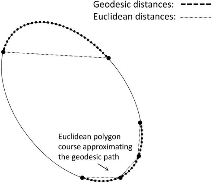
Schematic representation of geodesic distances (shortest paths on the manifold) vs. Euclidean distances measured in the ambient space ignoring the manifold structure. [24]
The linear approximation of geodesic distances on the manifold by an Euclidean polygon (see Fig. 1) can be described by a graph-theoretical shortest paths problem, which is detailed in [12] and [21]. The corresponding distance matrix \(D\in {\mathbb {R}}^{n\times m}\), where the entry \(d_{ij}\), \(i,j=1,\ldots ,m\), is the approximated geodesic distance between \(\mathbf {W}^{i}\) and \(\mathbf {W}^{j}\), is employed as input matrix for multidimensional scaling (MDS) [25, Section 14]. Based on the distance matrix D, MDS computes an embedding \(Y=\{\mathbf {y}^{1},\ldots ,\mathbf {y}^{m}\}\) with \(\left\| \mathbf {y}-\mathbf {y}^{j}\right\| \approx d_{ij}\) for \(i,j=1,\ldots ,m\), which is fine tuned by minimizing an additional loss function afterwards.
An approximate local inverse mapping from the low-dimensional space to the high-dimensional space is derived based on the set of low-dimensional vectors Y. For an arbitrary point \(\mathbf {y}^{*}\in {\mathbb {R}}^{d}\) let \({\mathcal {I}},\left| {\mathcal {I}}\right| =N\), denote the index set belonging to the N nearest neighbors of \(\mathbf {y}^{*}\). Due to Isomap, the nearest neighbors \(\{\mathbf {y}^{j}\ \vert \ j\in {\mathcal {I}}\}\) for a given vector \(\mathbf {y}^{*}\in {\mathbb {R}}^{d}\) within the embedding space \({\mathbb {R}}^{n}\) correspond isometrically to the nearest neighbors \(\{\mathbf {W}^{j}\ \vert \ j\in {\mathcal {I}}\}\) on the full-order solution manifold. Therefore, a linear approximation of \(\mathbf {y}^{*}\approx \sum _{j\in {\mathcal {I}}}a_{j}\mathbf {y}^{j}\) as a weighted sum of its N nearest neighbors is expected to yield good weighting coefficients that can be employed to build a linear combination of the corresponding high-dimensional snapshots on the full-order manifold. The weights vector \(\mathbf {a}=\left( a_{j_{1}},\ldots ,a_{j_{N}}\right) \in {\mathbb {R}}^{N},\ j_{i}\in {\mathcal {I}},\) for a linear approximation of \(\mathbf {y}^{*}\) by its neighbors is determined by the following optimality condition:
with
For a parameter combination \(\mathbf {a}^{*}\in {\mathbb {R}}^{N}\) the corresponding high-dimensional analogue \(\mathbf {W}^{*}\in {\mathbb {R}}^{n}\) is given by
Coupled with an interpolation model \(\mathbf {y}:{\mathcal {P}}\rightarrow {\mathbb {R}}^{d}\) formulated between the parameter space \({\mathcal {P}}\) and the low-dimensional space spanned by the set Y to predict \(\mathbf {y}^{*}=\mathbf {y}(\mathbf {p}^{*})\) at untried parameter combinations \(\mathbf {p}^{*}\in {\mathcal {P}}\setminus P\), a ROM is obtained which is capable of predicting full-order solutions. The sample data set for the interpolation model is given by \(\{(\mathbf {p}^{i},\,\,\mathbf {y}^{i})\}_{i=1}^{m}\).
4 Adaptive sampling strategies
Following the terminology of [26], various open and closed-loop adaptive DoEs are presented in this section. In contrast to static DoEs like Latin hypercube sampling (LHS), Halton sampling or full-factorial designs, these methods take advantage of prior knowledge that is incorporated into an error function \(e(\mathbf {p})\), \(e:\mathbb {R}^{d}\rightarrow \mathbb {R}\), representing a prior belief of the response accuracy of a ROM for a specific problem at a parameter combination \(\mathbf {p}\in \mathcal {P}\). All parameters used need to be independent from one another. The proposed methods only differ in their formulation of the error function \(e(\mathbf {p})\). Assuming that the error function \(e(\mathbf {p})\) is a good approximation to the actual error, a point \(\mathbf {p}^{*}\in \mathcal {P}\) with \(e(\mathbf {p}^{*})\ge e(\mathbf {p})\) for all \(\mathbf {p}\in \mathcal {P}\setminus \{\mathbf {p}^{*}\}\) has to be determined. To ensure that \(\mathbf {p}\in \mathcal {P}\) is fulfilled during the optimization process, the error function \(e(\mathbf {p})\) is multiplied by an indicator function \(\omega\):
where
The point \(\mathbf {p}^{*}\in \mathcal {P}\), which maximizes \(e_{\mathcal {P}}(\mathbf {p})\), i.e., \(\mathbf {p}^{*}={\text {argmax}}e_{\mathcal {P}}(\mathbf {p})\), is assumed to be the searched point.
To detail the approach of adaptive DoEs for ROMs in general, let the parameter space be given by the bounded set \({\mathcal {P}}\subset {\mathbb {R}}^{d}\) and let the discrete subset \(P_{{\tilde{m}}}=\left\{ \mathbf {p}^{1},\ldots ,\mathbf {p}^{{\tilde{m}}}\right\} \subset \mathcal {P}\) be a set of \({\tilde{m}}\in \mathbb {N}\) preselected parameter configurations. The corresponding snapshot set \(W_{{\tilde{m}}}=\left\{ \mathbf {W}^{1},\ldots ,\mathbf {W}^{{\tilde{m}}}\right\} \subset \mathbb {R}^{n}\) is given by the CFD solutions \(\mathbf {W}^{j}=\mathbf {W}(\mathbf {p}^{j})\) computed at the parameter configurations \(\mathbf {p}^{j}\in \mathcal {P}\), \(j=1,\dots ,{\tilde{m}}\). Moreover, let \(1\le i\le m-{\tilde{m}}\) be the number of the current iteration of the adaptive sampling (AS) process, where \(i,m\in \mathbb {N}\) and \(m>{\tilde{m}}\) is the number of desired snapshots.
The first step at iteration i is the update of interpolation models or ROMs, which are utilized to evaluate the error function \(e(\mathbf {p})\). Afterwards, the argument \(\mathbf {p}^{*}\in \mathcal {P}\) maximizing the error function \(e(\mathbf {p})\) has to be determined and the corresponding full-order CFD solution \(\mathbf {W}^{*}=\mathbf {W}(\mathbf {p}^{*})\) has to be calculated. The parameter configuration \(\mathbf {p}^{*}\) and the snapshot \(\mathbf {W}^{*}\) are added to the parameter and snapshot set, respectively. These sets are denoted by \(P_{{\tilde{m}}+i}\) and \(W_{{\tilde{m}}+i}\) after i iterations. This generic sampling process is detailed in algorithm 1 [24].
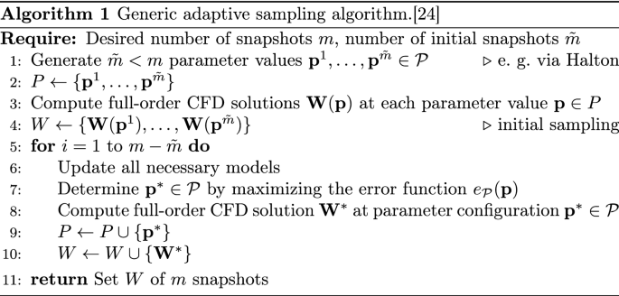
The following methods define different error function \(e(\mathbf {p})\) that can be substituted in algorithm 1 line 7.
4.1 Mean squared error (MSE)
Using Gaussian process based interpolation models \({\hat{f}}(\mathbf {p})\) (see [2, Section 2.4]) for POD+I or Isomap+I permits the computation of an error estimator, more precisely the mean squared error (MSE), which can be exploited to determine the parameter combination \(\mathbf {p}^{*}\in {\mathcal {P}}\) with highest uncertainty in the predictions of the model. The MSE in a Gaussian process is given as follows [2, 27]:
where \(\Psi \in {\mathbb {R}}^{m\times m}\) denotes the correlation matrix, \(\mathbf {\psi }\in {\mathbb {R}}^{m}\) the correlation vector and \(\sigma ^{2}\) the process variance. Note that \({\hat{s}}^{2}(\mathbf {p})\) reduces to zero at sample points \(\mathbf {p}\in P_{{\tilde{m}}+i-1}\). By omitting the constant value \(\sigma ^{2}\) in the sampling process the MSE error gets independent of the function values and hence only depends on the current set of sampled parameter combinations \(\mathbf {p}\in P_{{\tilde{m}}+i-1}\). Furthermore, the last term of the estimator is very small and therefore omitted here, which is a commonly accepted approach.
Maximizing
while dropping the aforementioned terms, leads to an explorative infill criterion, which is tantamount to filling the gaps between existing sample points \(\mathbf {p}\in P_{{\tilde{m}}+i-1}\) within the parameter space \({\mathcal {P}}\) [2, Section 3.2.2]. In each iteration, a full-order solution \(\mathbf {W}(\mathbf {p}^{*})\) is computed at \(\mathbf {p}^{*}={\text {argmax}}e_{\mathcal {P}}^{\text {mse}}(\mathbf {p})\in {\mathcal {P}}\) and added to the current database.
4.2 Leave-one-out cross-validation (LOO-CV)
A widely used method to estimate the prediction error of a model is the k-fold cross-validation (CV) [28, Section 7.10]. Hereby, the available data to fit the model is split in k ideally equal-sized parts. Then the model is fitted to \(k-1\) parts and validated based on the remaining part, i.e., comparing the predicted values to the actual values given by the left out samples. This is done for each of the k parts and the mean error is computed. Choosing \(k=\bigl |P_{{\tilde{m}}+i-1}\bigr |\) in iteration i, a leave-one-out CV is performed to compute the errors \(e_{j}=\bigl \Vert \mathbf {W}(\mathbf {p}^{j})-\hat{\mathbf {W}}(\mathbf {p}^{j})\bigr \Vert _{2}\) for \(\mathbf {p}^{j}\in P_{{\tilde{m}}+i-1}\), \(j=1,\ldots ,{\tilde{m}}+i-1\). Note that the POD-based prediction \(\hat{\mathbf {W}}(\mathbf {p}^{j})\) is based on the data set \(W_{{\tilde{m}}+i-1}\setminus \{\mathbf {W}(\mathbf {p}^{j})\}\). Hence, for each error computation \(e_{j}\) a POD has to be computed. Afterwards, a Gaussian process based interpolation model \({\hat{e}}:\,\mathbb {R}^{d}\rightarrow \mathbb {R}\) is formulated based on the data \(\{(\mathbf {p}^{j},e_{j})\}_{j=1}^{{\tilde{m}}+i-1}\) to estimate the error \({\hat{e}}(\mathbf {p})\) at untried parameter combinations \(\mathbf {p}\in \mathcal {P}\). To ensure that the error is zero at \(\mathbf {p}\in P_{{\tilde{m}}+i-1}\) the estimate is multiplied by Eq. (13):
4.3 CFD residual
In CFD the residual is used as a measure of convergence for the underlying problem. With this information a ROM prediction \(\hat{\mathbf {W}}\left( \mathbf {p}\right)\) at an untried parameter combination \(\mathbf {p}\) can be evaluated with respect to the underlying physical model. If the residual of a ROM prediction \(\mathbf{res}\left( \hat{\mathbf {W}}\left( \mathbf {p}\right) \right)\) is large, then the underlying physics are not resolved accurately. A new sample at \(\mathbf {p}\) would improve the model prediction in the area of \(\mathbf {p}\). Note that in contrast to the other adaptive sampling methods in this paper, the CFD residual methods must provide all the primitive variables of the complete flow field in order to evaluate the CFD residual. The primitive variables used for the governing equations are the density \(\rho\), the velocity components in all spatial directions (\(u_{x}\), \(u_{y}\), \(u_{z}\)) and the total energy E as well as the primitive variables corresponding to the chosen turbulence model used.
4.3.1 Residual only (Res)
Considering the cell volumes with the diagonal matrix \(\Omega\), the maximum error with respect to the \(L_{2}\)-norm for a certain flux residual \(\varphi\) is given with
For the investigations in this paper \(\varphi\) is set to the energy residual, since it has been shown that the energy residual provides the best results in a residual minimization context [29].
4.3.2 Residual with mean squared error (\(\text {Res}_{\text {MSE}}\))
In general, a ROM does not contain solutions that feature a zero residual—the error \(e_{{\mathcal {P}}}^{res}\) is not zero for any \(\mathbf {p}\in {\mathcal {P}}\). Similar to the leave-one-out cross-validation method the error \(e_{{\mathcal {P}}}^{res}\) is multiplied with Eq. (13) to ensure that the error is zero at a sample location \(\mathbf {p}^{j}\in {\mathcal {P}}\) with
4.4 Manifold filling
In the following section a brief introduction to the manifold filling based adaptive sampling strategy is summarized. A more detailed description can be found in [24].
Manifold learning methods try to preserve the topology of the underlying manifold \({\mathcal {W}}\) by inspecting the solutions \(W\subset {\mathcal {W}}\) (see Sect. 3.2). The approximately isometric embedding Y can then be exploited in the context of an adaptive sampling strategy by adding more solutions \(\mathbf {W}(\mathbf {p}^{*})\), \(\mathbf {p}^{*}\in {\mathcal {P}}\) in regions of the parameter space where fewer samples are located. A more even distribution of solutions in the manifold should be obtained [24]. Consequently the manifold \({\mathcal {W}}\) can be better approximated resulting in a more accurate ROM.
4.4.1 Maximum distance error (MDE)
Based on an initial embedding \(Y_{{\tilde{m}}}=\left\{ \mathbf {y}^{1},\ldots ,\mathbf {y}^{{\tilde{m}}}\right\} \subset \mathbb {R}^{d}\) using Isomap the coarser sampled regions within the embedding space are detected by a weighted sum of distances of the \(N\in \mathbb {N}\) nearest neighbors to \(\mathbf {y}(\mathbf {p})\) with
where \({\mathcal{I}},\left| {\mathcal{I}} \right| = N\), denotes the index set belonging to the N nearest neighbors of \(\mathbf {y}(\mathbf {p})\), \(d_\mathrm{min}(\mathbf {y}(\mathbf {p}))=\min _{j\in {\mathcal {I}}}\left\| \mathbf {y}(\mathbf {p})-\mathbf {y}^{j}\right\| _{2}\), \(d_\mathrm{max}(\mathbf {y}(\mathbf {p}))=\max _{j\in {\mathcal {I}}}\left\| \mathbf {y}(\mathbf {p})-\mathbf {y}^{j}\right\| _{2}\) and \(\left\| \mathbf {x}\right\| _{2}=\sqrt{\sum x_{i}x_{i}}\) being the euclidean distance of a vector \(\mathbf {x}\).
The to be optimized function is then given with
The above method will be referred to as maximum distance error (MDE).
4.4.2 Hybrid error (\(\text {HYE}_{5}\))
The hybrid error method \(\text {HYE}_{5}\) is based on the maximum distance error method MDE (see Sect. 4.4.1) and enhances the objective function Eq. (16) by a term that deals with the reconstruction error in iteration i of the N nearest neighbors. The relative error
for each \(\mathbf {y}^{j}\in Y_{{\tilde{m}}+i-1}\) is expressed by a prediction \(\hat{\mathbf {W}}(\mathbf {y}^{j})=\hat{\mathbf {W}}^{j}\) and the corresponding snapshot \(\mathbf {W}^{j}\). With all computed relative errors interpolation is used to approximate the relative error at \(\mathbf {y}\notin Y_{{\tilde{m}}+i-1}\) based on the data set \(\{(\mathbf {y}^{j},e^{\text {rel}}(\mathbf {y}^{j}))\}_{j=1}^{{\tilde{m}}+i-1}\). The to be optimized objective for the \(\text {HYE}_{5}\) method is
The error function \(e_{\mathcal {P}}^{\text {rec}}\) should only be used every k iterations (in the current work \(k=5\)). For the remaining iterations \(e_{\mathcal {P}}^{\text {dist}}\) should be used to obtain a homogeneously distributed manifold.
5 Test cases
The adaptive sampling strategies are evaluated with two test cases. Both use a two dimensional flow problem around an airfoil computing the snapshots \(\mathbf {W}^{i}\), \(i=1,\ldots ,m\) with the DLR flow solver TAU [30] using the RANS equations with the Negative Spalart-Allmaras turbulence model [31]. For each test case a small number of initial sample locations in the parameter space is obtained with the Halton sequence [32] which performed as the best one shot sampling method on similar problems in [33]. Furthermore, compared to a Latin-hypercube sampling, analogues to an adaptive sampling strategy it allows to iteratively add more samples which makes it easier to compare to the investigated strategies. The initial and iteratively added samples are used to compute a ROM+I based on POD (see Sect. 3.1) with the surface pressure distribution \(c_\mathrm{p}\) as the modeled variable.
The two test cases differ in the number of dimension of the parameter space \({\mathcal {P}}\). The first test case uses a symmetrical airfoil and two parameters, angle of attack \(\alpha\) and Mach number Ma, whereas the second test case also varies the geometry of the airfoil with three Class-Shape function Transformation (CST) parameters [34].
The performance of the adaptive sampling strategies is evaluated in each iteration i with respect to the resulting error \(e_{i}\) by comparing the ROM+I prediction of the surface pressure distribution \({\hat{c}}_{p}\left( \mathbf {p}^{i}\right)\) with a fully converged flow solution \(c_{p}\left( \mathbf {p}^{i}\right)\) for the same parameters with
and \(j=1,\ldots ,q\). The root mean square of the errors \(e_\mathrm{rms}=\frac{1}{q}\sqrt{\sum _{j}e_{j}^{2}}\) as well as the maximum errors \(e_\mathrm{max}=\max e_{i}\) and the variance of the errors \(e_\mathrm{var}={\text {var}}e_{i}\) are then used to evaluate the error for a distinct iteration.
The sample \(\mathbf {p_{i+1}^{*}}\) is determined by maximizing the error function (algorithm 1 line 7) using a brute force optimization within the parameter space.
5.1 Two dimensional test case
For the two dimensional test case the symmetrical NACA 64A010 airfoil as displayed in Fig. 2 is chosen.
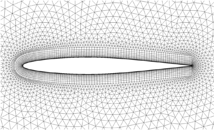
Detailed view of the NACA 64A010 airfoil with finite volume mesh
With the varying parameters angle of attack \(\alpha\) and Mach number Ma the parameter space \({\tilde{\mathcal{P}}}\) is defined by \({\tilde{\mathcal{P}}} = \left[ {0,7} \right] \times \left[ {0.5,0.8} \right]\) for \(\alpha \in [0,7]\) and \(\mathrm{Ma}\in [0.5,0.8]\). However, due to flow separation occurring for a combination of large angles of attack and Mach numbers the parameter space \({\tilde{\mathcal{P}}}\) is cut off approximately there where the glide ratio \(\frac{c_\mathrm{l}}{c_\mathrm{d}}\) is lower than 20 (see Fig. 3). The remaining feasible domain is denoted by \({\mathcal {P}}\).
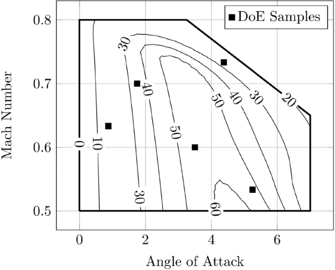
Glide ratio \(c_\mathrm{l}/c_\mathrm{d}\) of the NACA 64A010 airfoil in the investigated parameter space
The initial five samples \(\mathbf {p}^{1},\ldots ,\mathbf {p}^{5}\in {\mathcal {P}}\) for all sampling strategies are marked with \(\blacksquare\) in Fig. 3. Iteratively, each method adds 45 new samples in the prescribed parameter space \({\mathcal {P}}\) to end up with \(m=50\) snapshots in total. With the resulting snapshots a POD based ROM for the surface pressure distribution \(c_\mathrm{p}\) is computed and the predictions are compared against the high-fidelity solutions as described above.
5.2 Five dimensional test case
The five dimensional test case adds three geometrical CST parameters to the parameters angle of attack \(\alpha\) and Mach number Ma of the test case described above.
The upper and lower surface contour \(\zeta \left( \Psi \right)\) of a two dimensional symmetrical airfoil is describes in a CST parameterization with
with \(C_{N2}^{N1}\left( \Psi \right) =\Psi ^{N1}\left( 1-\Psi \right) ^{N2}\) being the geometric class and \(S\left( \Psi \right)\) the shape function. The variable \(\Psi =\frac{x}{c}\) normalizes the length of the airfoil with its chord. The last term in equation Eq. (20) allows the airfoil to have a trailing edge thickness. The shape function \(S\left( \Psi \right)\) can have various forms but is often chosen to be described with Bernstein polynomials of order \(N_{B}\) with
Applied to the three CST parameters of the five dimensional test case the order of the Bernstein polynomials is set to \(N_\mathrm{B}=2\). The base airfoil is chosen to be most similar to the NACA 64A010 airfoil of the two dimensional test case. Therefore an optimization process obtained the geometric class parameters N1 and N2 to be \(N1\approx 0.35\) and \(N2\approx 0.016\). Also, the last term of equation Eq. (20) is dropped since the NACA 64A010 has no trailing edge thickness. To obtain a new mesh for a parameter combination \(\mathbf {p}^{i}\) the reference mesh is deformed using radial basis function based on the methodology presented in [35].
A subset of the resulting geometry variations is displayed in Fig. 4.
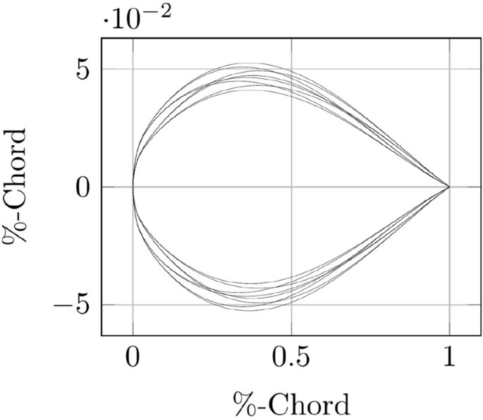
Resulting CST airfoil geometry variations on the corners of the parameter space
In contrast to the two dimensional test case the parameter space is not cut off in the angle of attack and Mach number domain (see Fig. 3), but forms a five dimensional hyper cube: \({\mathcal {P}}=\left[ 0,7\right] \times \left[ 0.5,0.8\right] \times \left[ 0.05,0.07\right] \times \left[ 0.09,0.11\right] \times \left[ 0.025,0.035\right]\). With 7 initial samples obtained by the Halton sampling method, the adaptive sampling strategies iteratively add 243 samples until 250 snapshots for each investigated method are available. Again, the resulting error inequation Eq. (19) is computed based on a fully converged flow solution for the same parameter combination.
6 Numerical results
The following section describes and discusses the findings of our work. In the first part the overall behavior and characteristics of the different sampling strategies are analyzed and compared against the one-shot Halton strategy. Next, the performance of all strategies is evaluated with respect to minimizing the modeling error by introducing new samples to the ROM+I. Finally an estimation of the total time savings is given.
6.1 Analyzing sampling strategies
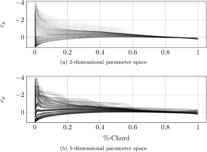
Various \(c_\mathrm{p}\)-distributions for the 2- and 5-dimensional test case
In Fig. 5, the \(c_\mathrm{p}\)-distributions resulting from high fidelity CFD simulations are displayed over the normalized cord-wise coordinate for varying parameters in the 2- and 5-dimensional test case. Contained in the plotted samples is the border of the parameter space with a course full factorial combination of all parameters. The spanned domain features subsonic and transonic flows with shocks occurring on the suction side of the airfoil. Especially the region of higher angles of attack and Mach numbers exhibits larger gradients and curvatures in the modeled \(c_\mathrm{p}\) response. It is therefore expected, that this critical region with its nonlinear effects should be more densely sampled in order to reduce the ROM+I model error [33].
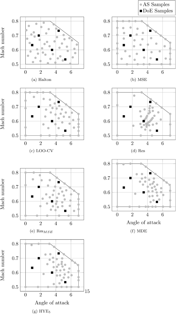
Sample locations after 45 iterations for all sampling strategies for the 2-dimensional test case
Figure 6 displays the sample locations after 50 iterations for all investigated methods for the 2-dimensional test case. All strategies were started with the five identical initial samples computed with the Halton sequence dented with a black square \(\blacksquare\). The Halton and MSE methods (Fig. 6a, b) equally distribute the samples in the sub- and transonic region of the parameter space without any preference for the previously identified critical high angle of attack and Mach number region. This is expected since the Halton DoE method is a one-shot strategy and the MSE method neglects any information provided by the function values and only operates on the sample locations in the parameter space (see Sect. 4.1). The only notable difference is that the MSE method also samples the border of the parameter space.
The methods depicted in (Fig. 6c–g) provide a more dense sampling in the critical parameter space region with differences in the space between sample locations (Fig. 6d, e) and the extent in which the critical region is identified.
Except for the Halton method, all adaptive sampling methods determine the location of the next sample in the parameter space based on a corresponding error function introduced in Sect. 4. The goal of these error functions is to detect the true modeling error and its global maximum is the location in the parameter space where the next sample is placed, computed via CFD and added to the ROM+I. By choosing the sample at the location in the parameter space with the highest error, the error reduction of the ROM+I is expected to be maximal. Figure 7 displays these normalized objectives for all investigated adaptive sampling strategies and marks the global optimum with a red cross.

Figure 7a shows the true ROM+I model error. It is computed based on 3643 high fidelity CFD simulations distributed in a full factorial manner within the bounds of the parameter space. It can be seen that the modeling error is lowest in the vicinity of sample locations. The border of the parameter space yields higher errors, especially in the high angle of attack and Mach number region. Figure 7b shows the error function for the MSE adaptive sampling strategy. As mentioned above, it is a space filling strategy. It values sampling locations only based on the distance to the current samples in the ROM+I. Consequently, it is paramount to first introduce samples on the border of the parameter space. Figure 7c shows the error function for the leave-one-out cross-validation adaptive sampling strategy. Here, the lower angle of attack and Mach number region yields potentially lower errors. This evaluation leads to a denser sampling in the critical regions in the parameter space. The same is true for Fig. 7d–g (see Fig. 6). By design of the method, Fig. 7f and g share for the first iteration the same error function.

Normalized initial error functions for the investigated adaptive sampling strategies
In Fig. 8a comparison of the leave-one-out cross-validation error function with and without an MSE term is analyzed.

Comparison of cross-correlation error function with and without MSE term
The main objective of the MSE term is to avoid too close sample placements in the parameter space. A comparison of Figs. 7a and 8a shows that the error function of the leave-one-out cross-validation without the MSE term does reflect the characteristics of the true model error. Consequently a new sample would roughly be introduced at \(p_{1}=\left( 4.5,0.75\right)\), which is in close proximity to an already existing sample in the ROM+I. This sample location would presumably not contribute as much of new information into the ROM+I as a sample chosen by the leave-one-out cross-validation with MSE term at \(p_{1}=\left( 0.0,0.8\right)\).
6.2 Error evaluation of sampling strategies
The main goal of an optimal sampling strategy is to introduce as much information with a single sample into the model as possible and consequently reduce the model error. For the two test cases, this reduction in error is evaluated based on 3643 samples \(\mathbf {p}^{j}\in {\mathcal {P}}\) in the 2 dimensional test case and 36125 samples for the 5 dimensional test case with \(j=1,\ldots ,3643\) or \(j=1,\ldots ,36125\) respectively. All samples \(\mathbf {p}^{j}\) are equidistantly distributed in the parameter space. The absolute errors of each resulting ROM+I in iteration i are computed for the \(k\in {\mathbb {N}}\) to be modeled \(\mathbf {c}_{p}\in {\mathbb {R}}^{k}\) values based on \(E_{i}=\left\{ \left. \text {abs}\left( {\hat{c}}_{p}^{i,j,k}-c_{p}^{i,j,k}\right) \right| \forall j,k\right\}\) with \({\hat{c}}_{p}^{i,j,k}\) being the \(c_{p}\) prediction of the \(k^{th}\) cell for the \(\mathbf {p}^{j}\) sample and \(c_{p}\) the corresponding CFD high fidelity solution. The ROM+I model error for the different adaptive sampling strategies is then compared based on the maximum error \(e_{i}^{max}=\max \left( E_{i}\right)\), the variance in error \(e_{i}^{var}=\text {var}\left( E_{i}\right) =\frac{1}{\left| E_{i}\right| ^{2}}\sum _{e\in E_{i}}\frac{1}{2}e^{2}\) and the root mean squared error \(e_{i}^{rms}=\sqrt{\frac{1}{\left| E_{i}\right| }\sum _{e\in E_{i}}e^{2}}\).
During the adaptive sampling process new samples are introduced to the ROM+I. These samples will reduce the local errors in the vicinity of the newly added samples in the parameter space. However, especially in the beginning of the adaptive sampling process, the global errors (\(e^{max}\),\(e^{var}\) and \(e^{rms}\)) could increase if the overall sampling is still too sparse. Since trends in error reduction are more relevant than the performance of an adaptive sampling strategy for a specific number of iterations, the error curves discussed are showing a moving averaged error \({\bar{e}}_{i}=\frac{1}{5}\left( e_{i-2}+e_{i-1}+e_{i}+e_{i+1}+e_{i+2}\right)\) of a kernel size of five with a reduced window size on the borders. This filters out irrelevant high frequency error fluctuations and allows to better compare the overall error reduction of each sampling strategy. It is apparent from Fig. 9, where the unfiltered and filtered data is plotted next to each other, that this approach does not diminish the generality of our findings.

Comparison of the unfiltered RMS error and the corresponding filtered moving average error of the Halton and LOO-CV adaptive sampling strategy for the two dimensional test case

Moving average RMS error of ROMs sampled with different adaptive sampling strategies for the two and five dimensional test case
Figure 10 shows the development of the filtered RMS ROM+I model error for an increasing number of snapshots for the 2- and 5-dimensional test case and all investigated methods. The starting RMS error after the initial DoE is the same for all adaptive sampling strategies in the corresponding test case, but larger in magnitude for the 5 parameter case relative to the 2 parameter case. This is due to the higher dimension and the resulting sparser sampling. The error is reduced significantly after the first number of iterations by all sampling strategies. It continues to further decrease, but at a slower rate than at the start of the adaptive sampling process. Figure 10c and d show a detailed view of the last iterations of the corresponding test case. Here, a quantitative difference between the sampling strategies can be observed. In both cases the Halton one-shot strategy performs worst while the \(\text {Res}_{\text {MSE}}\) strategy is best in the 2-dimensional test case and second best in the 5-dimensional test case.
Table 1 summarizes the results of all adaptive sampling strategies and both test cases for the three different error norms after all iterations have been included in the ROMs+I. Highlighted are the three best strategies for each error norm. It is evident, that the Halton one-shot strategy performs worst for all error norms and test cases while the \(\text {Res}_{\text {MSE}}\) method ranks high for all cases and error metrics. It always outperforms the Res adaptive sampling strategy. Between the manifold filling strategies the MSE and \(\text {HYE}_{5}\), the latter method obtains the better results.
6.3 Estimation of total time savings with adaptive sampling
The time needed to compute a ROM+I with an adaptive sampling process is dominated by two factors: First, the time needed to compute the error function of the adaptive sampling strategy and finding its maximum. Second, the time required for computing the next high fidelity CFD solution at the selected location in the parameter space (lines 7 and 8 in algorithm 1).

Wall clock time for computing the error function of the different sampling strategies for the 5-dimensional test case
Figure 11 shows on a logarithmically scaled ordinate the time needed to compute the error function for the investigated adaptive sampling strategies of the 5-dimensional test case on a \(3.2\text {GHz}\) CPU. It is obvious that the MSE method, which only operates on the sample locations in the parameter space, takes the least amount of time to compute the error function. The other methods depicted in Fig. 11 are dependent on the values of the used samples and take orders of magnitudes longer to compute the error function. For these methods the gradient or increase in time needed to obtain the error function is the most significant factor when it comes to performing an adaptive sampling strategy for a high number of samples. While the residual and manifold based methods share a similar gradient, the LOO-CV method has the highest increase in time. It is noteworthy to point out that the residual based methods highly depend on the interface type to the CFD solver. However, this factor would only have an influence on the absolute offset of the time and not its gradient.

Difference in number of samples needed for equivalent ROM+I filtered RMS error compared to Halton sampling strategy
Figure 12 can be analyzed in close conjunction with Fig. 10, as it displays the actual number of samples a ROM+I can be reduced by, compared to the Halton one-shot strategy, if the samples are located by the corresponding adaptive sampling strategy while maintaining the same level of RMS error. Compared to the one-shot strategy it is possible to reduce the number of samples by 22 with the \(\text {Res}_{\text {MSE}}\) method in the 2-dimensional test case and by up to 89 samples with the LOO-CV method in the 5-dimensional test case. In relative terms, this corresponds to a reduction of \(44\%\) and \(35.6\%\) of necessary samples to obtain the same error level for the corresponding test case.
7 Conclusion
A grand scheme for the adaptive sampling process is laid out and several different adaptive sampling strategies based on ROMs+I are introduced. The strategies differ in the way the error function is constructed, which is the basis for the decision where new samples are to be computed and introduced to the ROM+I. The sampling strategies investigated are: a Gaussian process based adaptive sampling method (MSE) which only operates on the parameter values, a leave-one-out cross-validation method (LOO-CV) that models the ROM+I error by splitting the available data in training and test sets, two residual based methods (Res, \(\text {Res}_{\text {MSE}})\), which model the ROM+I error by utilizing the CFD solver to evaluate the error of the predictions in the parameter space and two manifold based methods (MDE, \(\text {HYE}_{5}\)), which perform the decision making for the new sample with a space filling strategy but within an embedded manifold. The one-shot Halton sampling strategy is incorporated in the study to compare the adaptive sampling strategies to a response agnostic method.
The introduced strategies are applied to two test cases. Both test cases are based on the NACA64A010 airfoil and the ROMs+I model the normalized surface pressure distribution (\(c_{p}\)) on the airfoil surface. The first test case varies the angle of attack and Mach number in a transonic flow regime, while the second test case extends the first test case by also introducing three geometric parameters based on a CST parameterization resulting in a 2- and 5-dimensional parameter space.
The numerical results are divided into sections that deal with the resulting qualitative sample placements in the parameter space with the corresponding error functions, the quantitative error reduction obtained and an evaluation of the potential time savings an adaptive sampling process can achieve.
All methods reduce the error as new samples are introduced into the ROMs+I. As error norms the maximum error, the error variance as well as the root squared error (RMS) are used to evaluate the error reduction. Across both test cases and all error norms the \(\text {Res}_{\text {MSE}}\) method is one of the top three methods (see Table 1). The \(\text {HYE}_{5}\) as well as the LOO-CV method achieve robust and good results. Compared to the adaptive sampling strategies, the one-shot Halton strategy performs worst for all three investigated error norms. With respect to reduction of required samples for a given model quality, we showed that \(44\%\) or \(35.6\%\) fewer samples for the first and second test case respectively, are needed with the same global RMS error, if the sample locations are obtained by an adaptive sampling method. This clearly demonstrates the benefits of adaptive sampling strategies, compared to one-shot strategies, especially if the to be modeled process has non linear effects with respect to its parameters.
References
LeGresley, P., Alonso, J.: Investigation of non-linear projection for pod based reduced order models for aerodynamics. In: 39th aerospace sciences meeting and exhibit, p. 926 (2001)
Forrester, A., Sóbester, A., Keane, A.: Engineering Design Via Surrogate Modelling: A Practical Guide. Wiley, Hoboken (2008)
Liu, H., Ong, Y.-S., Cai, J.: A survey of adaptive sampling for global metamodeling in support of simulation-based complex engineering design. Struct. Multidiscip. Optim. 57(1), 393–416 (2018)
Loeppky, J.L., Moore, L.M., Williams, B.J.: Projection array based designs for computer experiments. J. Stat. Plan. Inference 142(6), 1493–1505 (2012)
Pholdee, N., Bureerat, S.: An efficient optimum latin hypercube sampling technique based on sequencing optimisation using simulated annealing. Int. J. Syst. Sci. 46(10), 1780–1789 (2015)
Halton, J.H.: On the efficiency of certain quasi-random sequences of points in evaluating multi-dimensional integrals. Numer. Math. 2(1), 84–90 (1960)
Beck, J., Guillas, S.: Sequential design with mutual information for computer experiments (mice): emulation of a tsunami model. SIAM/ASA J. Uncertain. Quantif. 4(1), 739–766 (2016)
Golzari, A., Sefat, M.H., Jamshidi, S.: Development of an adaptive surrogate model for production optimization. J. Petrol. Sci. Eng. 133, 677–688 (2015)
Viana, F.A., Haftka, R.T., Steffen, V.: Multiple surrogates: how cross-validation errors can help us to obtain the best predictor. Struct. Multidiscip. Optim. 39(4), 439–457 (2009)
Rumpfkeil, M., Yamazaki, W., Dimitri, M.: A dynamic sampling method for kriging and cokriging surrogate models. In: 49th AIAA Aerospace sciences meeting including the new horizons forum and Aerospace exposition, p. 883 (2011)
Blazek, J.: Computational Fluid Dynamics: Principles and Applications, 1st edn. Amsterdam, London, New York, Oxford, Paris, Shannon, Tokyo, Elsevier (2001)
Franz, T., Zimmermann, R., Görtz, S., Karcher, N.: Interpolation-based reduced-order modelling for steady transonic flows via manifold learning. Int. J. Comput. Fluid Dyn. 28(3–4), 106–121 (2014)
Zimmermann, R., Vendl, A., Görtz, S.: Reduced-order modeling of steady flows subject to aerodynamic constraints. AIAA J. 2014, 1–12 (2014)
Bui-Thanh, T., Damodaran, M., Willcox, K.: Proper orthogonal decomposition extensions for parametric applications in transonic aerodynamics. In: Proceedings of the 21th AIAA applied aerodynamics conference (2003)
Pinnau, R.: Model reduction via proper orthogonal decomposition. In: Model Order Reduction: Theory, Research Aspects and Applications (W. Schilders, H. van der Vorst, and J. Rommes, eds.), vol. 13 of Mathematics in Industry, pp. 95–109. Springer, Berlin Heidelberg (2008)
Zimmermann, R.: Gradient-enhanced surrogate modeling based on proper orthogonal decomposition. J. Comput. Appl. Math. 237(1), 403–418 (2013)
Holmes, P., Lumley, J.L., Berkooz, G.: Turbulence, Coherent Structures, Dynamical Systems and Symmetry. Cambridge University Press, Cambridge (1998)
Lucia, D.J., Beran, P.S., Silva, W.A.: Reduced-order modeling: new approaches for computational physics. Prog. Aerosp. Sci. 40(1), 51–117 (2004)
Van der Maaten, L., Postma, E., Van den Herik, H.: Dimensionality reduction: a comparative review. J. Mach. Learn. Res. 10, 1–41 (2009)
Cayton, L.: Algorithms for manifold learning. In: Univ. of California at San Diego Tech. Rep, pp. 1–17 (2005)
Tenenbaum, J., De Silva, V., Langford, J.: A global geometric framework for nonlinear dimensionality reduction. Science 290(5500), 2319–2323 (2000)
Gallot, S., Hulin, D., Lafontaine, J.: Riemannian Geometry. Springer, Berlin (2004)
Spivak, M.: A Comprehensive Introduction to Differential Geometry. Springer, Berlin (1999)
Franz, T.: Reduced-order modeling for steady transonic flows via manifold learning. In: PhD thesis, Deutsches Zentrum für Luft-und Raumfahrt (2016)
Mardia, K., Kent, J., Bibby, J.: Multivariate Analysis. Springer, Berlin (1980)
Garbo, A., German, B.: Comparison of adaptive design space exploration methods applied to s-duct cfd simulation. In: 57th AIAA/ASCE/AHS/ASC structures, structural dynamics, and materials conference, p. 0416 (2016)
Sacks, J., Welch, W. J., Mitchell, T. J., Wynn, H. P.: Design and analysis of computer experiments. Statistical science, pp. 409–423 (1989)
Hastie, T., Tibshirani, R., Friedman, J., Franklin, J.: The elements of statistical learning: data mining, inference and prediction. Math. Intell. 27(2), 83–85 (2005)
Zimmermann, R.: Towards best-practice guidelines for POD-based reduced order modeling of transonic flows. In: Proceedings of EUROGEN 2011 (C. Poloni, D. Quagliarella, J. Périaux, N. Gauger, and K. Giannakoglou, eds.), (Capua, Italy), CIRA—Italian Aerospace Research Centre (2011)
Schwamborn, D., Gerhold, T., Heinrich, R.: The DLR TAU-code: recent applications in research and industry, tech. report. In: European Conference on Computational Fluid Dynamics, ECCOMAS CFD 2006, (The Netherlands), Egmond and Zee (2006)
Allmaras, S. R., Johnson, F. T.: Modifications and clarifications for the implementation of the spalart-allmaras turbulence model. In: Seventh international conference on computational fluid dynamics (ICCFD7), pp. 1–11 (2012)
Kocis, L., Whiten, W.J.: Computational investigations of low-discrepancy sequences. ACM Trans. Math. Softw. (TOMS) 23(2), 266–294 (1997)
Rosenbaum, B.: Efficient Global Surrogate Models for Responses of Expensive Simulations. Springer, Berlin (2013)
Kulfan, B. M., Bussoletti, J. E., et al.: Fundamental parametric geometry representations for aircraft component shapes. In: 11th AIAA/ISSMO multidisciplinary analysis and optimization conference, vol. 6948, sn (2006)
Michler, A.K.: Aircraft control surface deflection using rbf-based mesh deformation. Int. J. Numer. Meth. Eng. 88(10), 986–1007 (2011)
Acknowledgements
The authors would also like to thank their colleague Dr. Marcel Wallraff for his help and support.
Funding
Open Access funding enabled and organized by Projekt DEAL.
Author information
Authors and Affiliations
Corresponding author
Additional information
Publisher's Note
Springer Nature remains neutral with regard to jurisdictional claims in published maps and institutional affiliations.
Rights and permissions
Open Access This article is licensed under a Creative Commons Attribution 4.0 International License, which permits use, sharing, adaptation, distribution and reproduction in any medium or format, as long as you give appropriate credit to the original author(s) and the source, provide a link to the Creative Commons licence, and indicate if changes were made. The images or other third party material in this article are included in the article's Creative Commons licence, unless indicated otherwise in a credit line to the material. If material is not included in the article's Creative Commons licence and your intended use is not permitted by statutory regulation or exceeds the permitted use, you will need to obtain permission directly from the copyright holder. To view a copy of this licence, visit http://creativecommons.org/licenses/by/4.0/.
About this article

Cite this article
Karcher, N., Franz, T. Adaptive sampling strategies for reduced-order modeling. CEAS Aeronaut J 13, 487–502 (2022). https://doi.org/10.1007/s13272-022-00574-6
Received:
Revised:
Accepted:
Published:
Issue Date:
DOI: https://doi.org/10.1007/s13272-022-00574-6