Abstract
The correlation filtering-based target tracking method has impressive tracking performance and computational efficiency. Nevertheless, a few issues limit the accuracy of the correlation filter-based tracking methods including the object deformation, boundary effects, scale variations, and the target occlusion. This article proposes a robust target tracking algorithm to solve these issues. First, a feature fusion method is used to enhance feature response discrimination between the target and others. Second, a spatial weight function is introduced to penalize the magnitude of filter coefficients and an ADMM algorithm is employed to reduce the iteration of filter coefficients when tracking. Third, an adaptive scale filter is designed to make the algorithm adaptable to the scale variations. Finally, the correlation peak average difference ratio is applied to realize the adaptive updating and improve the stability. The experiment’s result demonstrates the proposed algorithm improved tracking results compared to the state-of-the-art correlation filtering-based target tracking method.
Introduction
In recent years, target tracking has become a research hotspot in the computer vision domain due to its practical application in multiple fields, including video surveillance, human-computer interaction, driver less, and medical image analysis [1,2,3]. Target tracking requires providing the target size and position information in the initial frame, then predicts the accurate size and the position of the target in subsequent frames of the video sequence. Despite the remarkable progress made in target tracking technologies in the past few decades, a few associated limitations remain unresolved, which include scale variations, background clutter, motion blur, among others. Bolme et al. [2] first applied correlation filtering in the tracking field, and proposed a new filter, namely minimum output sum of squared error filter (MOSSE) [4] to find the largest response of tracking target. The Exploiting circulation structure of Tracking-by-detection with Kernels (CSK) [5] algorithm adds dense sampling and kernel mechanisms based on MOSEE to increase the tracking frame rate from 20FPS to 400FPS. Joao et al. [4] proposed the Kernel Correlation Filter algorithm that improved the CSK algorithm by extending the HOG feature of the multi-channel gradient. Martin Daniella et al. [6] designed a color names (CN) feature and added multi-channel color features to the CSK algorithm. Poria et al. [7] identify important features of rough theory to find a higher accuracy in retrieval results. Reza et al. [8] proposed an edge calculation method to solve the problem of the concepts of the fuzzy similarity relation and homogeneity region. Those archived good results.
Despite the apparent advantages of high speed in correlation filtering algorithms, there is still scope for improvement. The first area for consideration is that the target deformation in the tracking process leads to unstable tracking. The traditional KCF and DCF [4] algorithms use the HOG feature [9] as the sample feature, showing strong stability for phenomena like motion blur and illumination change. But these model relies heavily on the contour structure of the tracking target. Consequently, the algorithm becomes extremely sensitive to object deformation leading to unstable tracking results. The second area for consideration is the boundary effect of samples caused by circular shift of the center image block. In the training phase, while the dense samples are obtained by the circular shifting of the center image block, making only the center samples accurate, the others have displacement boundaries leading to the fact that even the trained classifier cannot accurately track the object moving rapidly. The third area for consideration is the lowering of the tracking accuracy due to the non-scalability of the target scale as per the target size. In the target tracking process, both the reduction and expansion of the target scale cause the tracking drift by including a large amount of background information and containing only part of the target information, respectively, in the selected image block. The fourth area for consideration is target occlusion. In target tracking, the occluded target causes drift in the tracking results, which affect the target training model to a certain extent. Thus, with longer occlusion time, the tracking fails. This paper mainly provides solutions to the above discussed four limitations of correlation filtering algorithms. In summary, the main contributions of this paper are as follows: (1) A feature fused by HOG, CN, and HSV is to enhance feature responses discrimination and improve the stability of tracking when the scene is deformed or lighting changes.

Algorithm flowchart. The algorithm structure is roughly divided into three main parts: (1) feature extraction and fusion, (2) template and response calculation and (3) template update
(2) A spatial regularization weight is set according to the location information of training samples and the target space. And a spatial weight function is proposed to penalize the magnitude of the filter coefficients of ADMM [10] to reduce iteration of filter coefficients, weaken the boundary effect to keep the efficiency of tracking.
(3) An adaptive scale filter with a 7-scale pool is designed, which makes the algorithm adaptable to the scale variations.
(4) The correlation peak average difference ratio is applied to estimate the state of occlusion, which can realize the adaptive updating of the tracking model and improve the stability when the target occlusion.
Related work
Despite the correlation filtering based target tracking method achieved remarkable progress, there are a few limitations remain unseasoned, which include target de-formations, boundary effects, scale variations and target occlusion. Researchers put a lot of efforts to solve these issues.
For the target deformation, Poria et al. [7] identify important features of rough theory to find a higher accuracy in retrieval results. Gupta et al. [11] proposed a RE-SiamNets to circumvent the adverse effect of rotation. The SiamNets allow estimating the change in the orientation of object in an unsupervised manner. Joao et al. [3] proposed an algorithm (CN) based on color space to limit the scope of the problem. As color features only focus on color changes and are not sensitive to contour changes, they show strong robustness to target deformation. This algorithm extends the RGB color space and proposes CN space, with eleven channels (named black, blue, brown, gray, green, orange, pink, purple, red, white, and yellow). Bertinetto et al. [12] improved this tracking algorithm from the aspect of feature fusion HOG feature training the correlation filter and the color histogram are used for obtaining a tracking score and the statistical score, respectively, and are fused to generate the final response image and estimate the target position. This feature fusion improves the accuracy of the tracking algorithm but also makes the calculation slightly more complicated. Ma et al. [13] introduced depth features based on correlation filtering and designed a tracker (HCFT) based on multi-layer convolution features With the depth features being are more robust than the common features. VGG16 [14] was used to extract the output features of conv3-4, conv4-4, and conv5-4 layers, as well as train the respective correlation filters. During target tracking, the 3-layer features of the search area are the input to the corresponding correlation filter, and the response image is generated by adding the weights, and the target is located through the maximum position.
For resolving the boundary effect problem, the solution of most algorithms is to add a cosine window on the image to weaken the influence of image boundary on the result, as KCF. The influence of the boundary effect remains weak, as long as the center part of the shifted image is reasonable. However, with an increasing number of reasonable samples, the validity of all training samples cannot be guaranteed in this method. Besides, the addition of a cosine window can make the tracker block the background information and only accept part of the valid information, thereby reducing the discriminating ability of the classifier. Danelljan et al. proposed a spatial constrained correlation filter (SRDCF) [15], with the filter coefficients mainly concentrated in the central region by adding weight con-straints. Lukei et al. [16] proposed a critical correlation filter CSR-DCF for reliable channel and space. Yan et al. [17] propose a novel, flexible and accurate refinement module called Alpha-Refine, which exploits a precise pixel-wise correlation layer together with a spatial-aware non-local layer to fuse features and can predict three complementary outputs: bounding box, corners and mask. In the proposed filter, the binary mask is obtained by using spatial reliability for adaptive selecting the target region easier to track and thus, reduce the boundary effect. CF+CA [18] points out that the negative samples, used for correlation filtering training, are obtained only by cyclic displacement of positive samples, which limits the background discrimination ability of the trained classifier. Therefore, negative samples collected around the positive samples are introduced in training to improve the tracking accuracy.
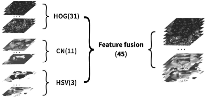
A fusion features provides a 45-dimensions including 31-dimensional HOG feature, 11-dimensional CN feature and 3-dimensional HSV feature

Fusion response graph. The single feature response graph being affected by a large amount of surrounding noise impacted accurate distinguishing of the target, while the feature response after fusion depicted a stronger discrimination between target and others
To solves the impact of scale variation on tracking performance, the adaptive scale variation correlation filter tracker (SAMF) [19] and scale judgment space tracker (DSST) [20] introduced scale estimation in KCF. SAMF [19] with 7-thick scales is used in a translation filter to detect multi-scale image blocks and selects the translation position and target scale corresponding to the largest response value. DSST [20] simultaneously trains the translation filter and the scale filter, respectively using 35 fine scales. At the on-set, the translation filter and the scale filter are used for position estimation and scale estimation, respectively. Most popular algorithms use these two scales to estimate position and scale.
For the target occlusion, Zhang et al. [21] used the kernel gray histogram as the description feature tracking each component of the target. It not only increases the robustness to occlusion but also solves the problem of non-rigid deformation of the target. Liu et al. [22] proposed a modeling method for unknown parts using hidden variables By extending the online Pegasus algorithm to the structured prediction of hidden variables of various parts, this method provides a better tracking effect than the best contemporary linear and nonlinear kernel tracker. Harley et at. [23] propose an unsupervised method for detecting and tracking moving objects in 3D, in unlabeled RGB-D videos. The constraint of ensemble agreement helps combat contamination of the generated pseudo-labels, and data augmentation helps the modules generalize to yet-unlabeled data.
Proposed method
The proposed methods is illustrated in Fig. 1, which is composed of three components. (1) Feature extraction. The HOG, CN, HSV features on target prediction area and candidate area are extracted, then fuse the feature to obtain the feature template. (2) Temple and response calculation. The response value of the template is calculated, and the credibility of the template is calculated by the correlation peak difference ratio. (3) Model update. If the credibility of the template is high, the template is updated. If it is low, the previous frame template is retained.
Feature fusion
A feature fusion method based on HOG, CN, and HSV is used to enhance feature responses discrimination and improves the stability of the target tracking. HOG feature that stable for light, which consists of 18 direction-sensitive channels, 9 direction-insensitive channels, 4 texture channels, and 1 zero channel [24]. The CN feature is the low dimensional adaptive extension of a color attribute, which is the language label commonly used to describe color [25]. HSV contains hue, saturation, and intensity information. Due to more similarity with human visual characteristics, HSV color space performs better than the RGB color space in visual tracking. The proposed method fused the HOG feature to represent the gradient change, the CN color space to represent color information, and the HSV space to obtain more detailed information. HOG feature is 31-dimensional (except for zero channel), CN feature is 11-dimensional (RGB colors map to eleven basic colors, namely, black, brown, gray, green, orange, pink, purple, red, blue, white, and yellow), and HSV feature is 3-dimensional. A fusion features provides a 45-dimensions integration feature as shown in Fig. 2. Figure 3 presents the response graphs for both single feature and fusion feature that shows the discrimination between target and others stronger.
Spatial regularization based on ADMM
In the KCF correlation filtering algorithm, to obtain the optimal classifier under the minimum square error [26], the circular shift sample is used to train the classifier, and Eq. 1 defines the training process loss function.
where \({\psi _t}\) is the training error for the first t frame classifier, t is the current frame number, i is the history frame serial number, \({x_i}\) is the first i frame of input samples, \(f({x_i})\) is the response score after the input sample of the i-th frame, \({y_i}\) is the expected response of the sample in the i-th frame, omega is the filter coefficient for training, j is the number of channels of the filter, \({a_i}\) is the frame weighting factor of classifier learning, d is the classifier dimensions, and \(\lambda \) is a constant regularization factor for over-fitting prevention.
It can be noted that the regularization factor \(\lambda \) is constant in the training process that treats the sample in the background area as the sample in the target area. However, in practical tracking, the target area is much more important than the background region. Thus, the regularization weight of the target area sample should be less than the background part. The paper introduced the spatial regularization weighting factor \(\theta \), building the spatial regularization correlation filter for weakening the interference of the background region, and improving the classification ability of classifiers in a cluttered background. Simultaneously, the use of this characteristic expands the search area and solves the issue of target loss due to rapid movement.
The original formula, after the introduction of the weight factor \(\theta \), is represented in Eq. 2
Here \(\odot \) is the dot product operation for \(\theta = \sqrt{\lambda }\), and the remaining parameters are similar to Eq. 1. The regularized weight is defined by Eq. 3.
Where m and n represents the offset of the cyclic sample, \({\theta _{base}}\) represents the constant basic weight of spatial regularization, and \({\theta _{shift}}\) represents the regularized weight offset of the training sample and is defined Eq. 4.
\({\rho _{width}}\) and \({\rho _{height}}\)represent the width and height of the search image, respectively. \( {\theta _{width}}\) and \({\theta _{height}}\)represent the weighting factors in the horizontal and vertical directions, respectively. Equation 11 depicts that the distance between the training sample and the target center is directly proportional to the value of \({\theta _{shift}}\), i.e., the greater the regularization weight of the background region, the smaller the weight of the target region.
Find the solution for the filter coefficient \(\omega \), a key issue in the correlation filtering algorithm. Advancements in the related tracker filters, including CFLB [27] with the BACF [26] algorithm in the training of the filter, have introduced the space constraints in handling the boundary effect. Although this algorithm has solved the issue of the boundary effect, it has made the filter model more complex, slowed the computing speed, and made the computing speed advantage less apparent in the correlation filtering algorithm.
The alternating direction multiplier method (ADMM) is proposed in this paper to solve the correlation filter. ADMM divides a large optimization problem into multiple sub-problems to obtain the solutions. The approximated solution of the filter can be quickly obtained by iteration of the sub-problems.
ADMM algorithm, in general, is used to solve the following form of minimization problem (Eq. 5.):
The augmented Lagrange function of this problem is defined as Eq. 6.
The augmentation of the augmented Lagrangian function is to add a square regular term to the Lagrangian function. The main purpose of introducing the augmented term is to make f as long as a convex function and to ensure its convergence. Then L is solved by the dual ascent method. The dual ascent method is (Eq. 7):
The classic ADMM algorithm framework is as follows: Initialize \({y^0}\), \({\varsigma ^0}\),\(\mu > 0\); The alternating direction in the ADMM algorithm is to modify the above dual ascending problem (x, z iterates together) to iterate x, z alternately, the iterative steps are as follows: Eq. 8
If the termination condition is fulfilled, the iteration is stopped, presenting output results or return to continue the iteration. Equation 2 is converted to the augmented Lagrangian function form. As ADMM iteration requires two variables, constructed as auxiliary variable and set and then converted Eq. 2 is represented as Eq. 9,
Converting the above equation to the frequency domain (Eq. 10),
where \(\wedge \) represents the Fourier transform of the variable, for example, the discrete Fourier transform of a one-dimensional signal a is represented as \({\hat{a}} = \sqrt{t} Fa\), F represents the orthogonal Fourier transform matrix of size \(t \times t,{\hat{y}} = [{\hat{y}}(1),{\hat{y}}(2),...,{\hat{y}}(t)]\), \({\hat{X}} = [diag{({{\hat{x}}_1})^T},...,diag{({{\hat{x}}_d})^T}]\) with the size \(t \times dt\hat{\beta }= [{\hat{\beta }} _1^T,...,{\hat{\beta }} _d^T]\),and \(h = [h_1^T,...,h_d^T]\) is a matrix composed of multi-channel cyclic samples with the size \(dt \times 1\) Thus, the Augmented Lagrange expression is as Eq. 21:
Here \(\mu \) is the penalty factor and \({\hat{\varsigma }} = {[\hat{\varsigma }_1^T,...,{\hat{\varsigma }} _K^T]^T}\) is the Lagrange vector of size \(dt \times 1\) in the Fourier domain. The ADMM algorithm can be used to solve the above equation iteratively according to Eq. 8 and every sub-problem \(\omega \) and \({\hat{\beta }}\) has a closed-form solution.
For sub-problem \(\omega \) the solution formula is Eq. 12
Here \(\varsigma = \frac{1}{{\sqrt{t} }}{F^{ - 1}}{\hat{\varsigma }} \) and \(\beta = \frac{1}{{\sqrt{t} }}{F^{ - 1}}{\hat{\beta }}\). Due to the linear nature of the discrete Fourier trans-form, each channel in the arrays \(\{ {\varsigma _1},...,{\varsigma _d}\}\) and \(\{ {\beta _1},...,{\beta _d}\}\) can be solved separately in the Fourier domain and the computational complexity of Eq. 12 is \( O(dt\log (t))\).
For sub-problem \({\hat{\beta }}\) the solution formula is Eq. 13:
The complexity of directly solving this equation is \(O({t^3}{d^3})\), as each ADMM iteration needs to solve\({\hat{\beta }}\), it significantly affects the real-time performance of the algorithm. However, sample a represents \( {\hat{X}}\), which is a banded sparse matrix. Accordingly elements of the array \({\hat{y}}(s) = [{\hat{y}}(1),{\hat{y}}(2),...,{\hat{y}}(t)]\) are only related to the k-th element of arrays \({\hat{x}}(s) = {[{{\hat{x}}_1}(t),...,{{\hat{x}}_k}(t)]^T}\) and \({\hat{\beta }} (s) = {[conj({{\hat{\beta }} _1}(t)),...,conj({{\hat{\beta }} _k}(t))]^T}\).The operator conj is the complex conjugate applied to complex number vectors. Therefore,\(\hat{\beta }\) the above equation can be represented as,\({\hat{\beta }} (s)\), \(s = [1,...,t]\), where t is independent small targets.
Here, \( {\hat{\omega }} (s) = [{{\hat{\omega }} _1}(s),...,{{\hat{\omega }} _k}(s)]\), \({{\hat{\omega }} _k} = \sqrt{t} F{\omega _k}\).
The computational complexity of Eq. 13 is \(O(t{d^3})\) due to the issue of dealing with the t independent \(K \times K\) linear systems. The d dimensional variables in the de-nominator and use of the Sherman-Morrison formula(\( {(u{v^T} + A)^{ - 1}} = {A^{ - 1}} - {({v^T}{A^{ - 1}}u)^{ - 1}}{A^{ - 1}}u{v^T}{A^{ - 1}}\)) for acceleration makes \(A = \mu t{I_k}\) and \(u = v = {\hat{x}}(s)\). Thus, the original formula can be simplified as Eq. 16,
Here,\({{\hat{S}}_x}(s) = {\hat{x}}{(s)^T}{\hat{x}}, {{\hat{S}}_\varsigma }(s) = {\hat{x}}{(s)^T}{\hat{\varsigma }} \),\({{\hat{S}}_\omega }(s) = {\hat{x}}{(s)^T}{\hat{\omega }}\),and\( b = {{\hat{S}}_x}(s) + \mu t\). Therefore, the computational complexity of the formula is reduced to O(td).
The Eq. 17 is iterative update:
where \({{\hat{\beta }} ^{k + 1}}\) and \({\omega ^{k + 1}}\) are the current solutions to the above sub-problems at iteration \(k + 1\) within the iterative ADMM. Thus, \({{\hat{\omega }} ^{k + 1}} = \sqrt{t} F{\omega ^{k + 1}}\) and \({\mu ^{k + 1}} = \min ({\mu _{\max }},\alpha {\mu ^k})\). The filter parameter \({\hat{\beta }} _t^j\) is obtained through the ADMM iterative optimization solution, and the change of tracking target position is estimated through the target response graph of the standard correlation filter used in tracking. Thus, the target output response in the time domain is as Eq. 18:
Scale adaptive scheme
The size of the target template remains fixed for most of the tracing methods. Thus, to deal with scale variation, an extension of scale-space from countable integer space to uncountable floating point space is proposed. Assuming that the size of the original image in the template is \({s_k}\), the different scale d form scale pool \(S = \{ {d_1}{s_k},{d_2}{s_k},...,{d_d}{s_k}\}\) is defined at the track. The d image blocks of different sizes according to s are taken in the new frame, and then through the bilinear interpolation method, the image block is adjusted for the same dimensions as the initial frame template \({s_k}\). Figure 4 depicts the specific process.

Sampling and adjustment process. (1) In the new frame of image, sample the image by sliding window according to d scales of different scales in S, and calculate the sample response of each scale, so as to determine the candidate regions of different scales. (2) Adjust these candidate area image blocks to the same dimension as the initial frame template by bilinear interpolation. (3) Perform feature extraction on the candidate ar-ea image blocks
We have specially trained a scale filter in the algorithm to estimate the scale of the target. The method of sliding window sampling is used to sample candidates with different scales in the scale pool, and then calculate separately the response value. The scale of the new frame target is updated according to the value of the scale with the largest response in the input scale pool, which improves the adaptability to changes in the scale of different targets, thereby achieving adaptive update of the scale. The step of target candidate box is calculated by Eq. 19,
Here \({z^{{d_i}}}\) is the image block detected of size \({d_i}{s_k}(i = 1,..,d)\) in a new frame. The response graph infers the moving steps of the target, and thereby, the corresponding real displacement deviation is the result of multiplication with the resulting displacement d.
Model update strategy based on high confidence
The current target tracking algorithm updates the model in almost every frame, regardless of the accuracy of the target detection. In the case of an inaccurate new tracking result, the result updates the model and pollutes it, which leads to tracking drift. In this algorithm, the HSV feature, HOG feature, and CN feature are combined for the target tracking. As the final feature dimension is very high, quite a lot of parameters need to be updated every time to update the model, which is quite time-consuming. Thus, model updating with every frame predictably slows the speed.
Therefore, the model update strategy based on high confidence solves the pollution problem of the model, improves the robustness of the tracking algorithm to occlusion and other issues, improves the tracking speed, and prevents over-fitting.
The actual use of KCF revealed that with the blocking of the target, the tracking result drifts, and the longer blocking time fails the tracking. The KCF [4] updates the model for every frame without considering the target blocking, and so with the blocked target, the tracking model gets polluted causing target loss. It infers that only when the part in the target box of the current frame has high confidence (the target is not obscured or blurred), the model could be updated. Therefore, the method of judging the sample confidence is the problem research problem of this chapter. Wang [28] concluded, through multiple KCF experiments, that the response profile of KCF has only one distinct peak and its overall distribution represents a two-dimensional Gaussian distribution, approximately. Thus, when a complicated situation occurs in the tracking process (especially occlusion, loss, blur, and so), the response graph oscillates violently.
The peaks and fluctuations in the response graph reflect the confidence of tracking results to some extent. The perfect matching of the detected with the correct target results in the ideal response graph with only one peak, and other areas tend to be smooth. The higher the correlation peak, the better is the positioning accuracy. In case of inaccurate positioning, the response graph oscillates violently, and its shape becomes significantly different from that of the correct match. Thus, this paper proposes a judgment formula CPMDR (Eq. 20):
Where \({f_{\max }}\) is the maximum value of the response graph, \({f_{\min }}\) is the minimum value of the response graph, and \({f_{m,n}}\) is the value of the response graph at (m, n).
The Correlation Peak Mean Difference Ratio (CPMDR) reflects the fluctuation of the response graph. When CPMDR is below a certain threshold, the target is judges as lost in the tracking process, obscured, or out of sight.
In traditional KCF tracing, the simple model update method used is as Eq. 21:
Here, \(\eta \) is the update rate of the model. According to this method, every frame for the classifier is to be updated. Once tracking fails, it cannot continue tracking. The proposed solution is to use the updating strategy of the learning rate adaptive high confidence model. To prevent the model from being contaminated, when the target area is blocked, the target model must not update. When the CPMDR value exceeds a certain threshold, the model can update. By setting the model update rate to be positively correlated with the CPMDR value, \(\eta = {\eta _1}(1 - \frac{1}{{CPMDR}})\) can be made. With \({\eta _1}\) set to 0.02, the updated adaptive model is Eq. 22:
This updated model calculates, \({\hat{\beta }} (s)\), \({{\hat{S}}_x}(s)\), \({{\hat{S}}_\varsigma }(s)\), and \({{\hat{S}}_\omega }(s)\). As measured by the experiment, when the CPMDR value is greater than 50, it identifies as accurate tracking, so the threshold is set as 0.0196. Figures 5 and 6 are comparison to Basic KCF and advanced method.

a The result of Basic KCF algorithm tracking. b The result of KCF algorithm tracking with high confidence model update strategy added. The comparison of the two sets of pictures reveals that the KCF algorithm with a high-confidence model update strategy is better than the basic KCF algorithm. As the improved KCF algorithm does not update the model when it is occluded, the model is not contaminated. Besides, after the target reappeared, the algorithm tracked the target again
The comparison of the two sets of pictures reveals that the KCF algorithm with a high-confidence model update strategy is better than the basic KCF algorithm. As the improved KCF algorithm does not update the model when it is occluded, the model is not contaminated. Besides, after the target reappeared, the algorithm tracked the target again.
Experiments
The experimental configuration
The proposed algorithm is implemented in MATLAB R2014a with a tracking speed of 12 frames per second. The experimental platform is configured in the following manner, the operating system is 64-bit Windows 7, the memory is 16 GB, the CPU is Intel i7-8700 k (6 core 3.7 GHZ), and the graphics card is NVIDIA GeForce GTX 1060.
The basic parameters of the experiment are as follows: The HOG feature uses a \(4 \times 4\) pixel cell size, the scale pool size is 7, and the scale factor \(S = [0.97,0.98,0.99,1.00,1.01,1.02,1.03]\).The search area is \({4^2}\) times the target area, the regularized base weight \({\theta _{base}}\) is 0.1, and the weight factors \({\theta _{width}}\) and \({\theta _{height}}\) are 3. For ADMM optimization, the iterations are 2 and the penalty factor \(\mu \) is 1. In iteration \(k + 1\), the penalty factor is updated by \({\mu ^{k + 1}} = \min ({\mu _{\max }},\alpha {\mu ^k})\), among them \(\alpha = 10\) and \({\mu _{\max }} = {10^3}\). The threshold of the target template learning rate is 0.0196.
The OTB50 standard target tracking test set [28], containing 50 video sequences, tests the proposed algorithm. The complete demonstration of the tracking effect of the proposed algorithm is through a comparison of selected 9 relevant algorithms for the same dataset. These algorithms are, ECO [29], SRDCF [30], STAPLE-CA [12], SAMF [18], DCF-CA [31], KCF [4], STRUCK [32], TLD [32], and CT [33]. Among them, CF [4], STRUCK [32], TLD [10], and CT [33] are the best classical algorithm from the OTB benchmark test. ECO [29], SRDCF [30], STAPLE-CA [12], SAMF [18], DCF-CA [31] are the best tracking algorithms based on correlation filtering, and ECO is also a classical algorithm combining correlation filtering and deep learning.
Quantitative comparisons
Overall performance
A comprehensive evaluation of the tracking results, in the following two ways, assesses the performance of algorithm. (1) The success rate for distance error; If in a specific frame, the distance error between the tracking algorithm and the manually calibrated tracking results is less than a certain threshold, then that frame is regarded as successful. (2) The success rate for coincidence degree; If in a specific frame, the coincidence degree between the tracking algorithm and the manually calibrated tracking results is larger than a certain threshold, then that frame is regarded as successful.
Figure 7 is the success rate schematic diagram of tracking OTB50 test video, (a) is the precision plot, and (a) is the success plot. In (a), the horizontal axis represents the threshold of the distance error, and the vertical axis represents the ratio of the number of frames with the distance error less than the threshold value to the total number of frames. The number after the title indicates the number of videos containing the tracking feature in the test video. The number after the algorithm indicates the area under the curve (AUC) with the coordinate axis, and OPE (One-Pass Evaluation) is the complete segment of the one-time tracking video. The range error success rate reflects the accuracy of the tracking position. (b) Shows the success rate of the degree of coincidence, where the horizontal axis represents the threshold of the degree of coincidence, and the vertical axis represents the ratio of the number of frames with the degree of coincidence greater than the threshold value to the total number of frames. The success rate of coincidence degree reflects the overall tracking accuracy of the algorithm.
In addition, statistics of calculation time among the competitors and proposed is show in the Table 1, which illustrates that the proposed method performance best in the accuracy of tracking with a short time.

The comparison success rate on the OTB-50 test video (red line is ours)
Figure 7 depicts the accuracy and success rate scores of the proposed algorithm are 0.853 and 0.821, respectively, which is best among the ten tracking algorithms compared. The accuracy and success rate increase by 11.3 and 19.8%, respectively, as compared to the classic KCF [4] algorithm. Compared to the second ECO [29] algorithm increase is by 0.5 and 1.8, respectively. Among the top five algorithms, SAMF [18] and STAPLE-CA [12] are the improved versions of the KCF [4]. SAMF [18] adds an adaptive scale transformation to KCF [4], and STAPLE-CA [12] adds the feature fusion and combination of CN and HOG to KCF [4]. ECO [29] and SRDCF [30] are the improved versions of the DCF [31] tracker with contextual awareness and taking background information into account in its model appearance. SRDCF adds spatial regularization based on DCF [31]. ECO [29] integrates the functions of CNN [34] into SRDCF [30] and realizes the acceleration of the algorithm. The proposed algorithm is SRDCF-based, with the addition of the feature fusion and the model update based on confidence. Besides, the introduction of the iterative acceleration calculation in the ADMM algorithm reduces the computational complexity and improves the accuracy of tracking and the calculation speed. Experimental results show that the proposed algorithm has higher tracking accuracy and robustness.
Performance analysis based on video attributes
To better analyze the performance strengths and limitations of the algorithm proposed in this paper. Figures 8 and 9 depicts the recorded accuracy scores and success rate scores of 10 algorithms in 11 video attributes. These 11 attributes include (a) fast motion, (b) background clutter, (c) motion blur, (d) deformation, (e) illumination variation, (f) in-plane rotation, (g) low resolution, (h) occlusion, (i) out-of-plane rotation, (j) out of view, (k) scale variation. In the accuracy score, the proposed algorithm scores among the top four algorithms, with six out of eleven attributes ranked in the top two. In the success rate score, the proposed algorithm is best in all the eleven attribute scores, with eight scores in the top two and five scores ranked first.

Accuracy score curve of 11 algorithms on an OTB-50 dataset
Figure 9 shows the recorded success plot of ten algorithms for the eleven video attributes, simultaneously. The eleven attributes include illumination variation, scale variation, occlusion, deformation, motion blur, fast motion, in-plane rotation, out-of-plane, rotation, out of view, background clutter, and low resolution. In the success rate score, eight of the eleven attributes of the proposed algorithm is in the top two, and five are ranked first.

The success rate score curve of 11 algorithms in the OTB-50 dataset

Comparison of tracking effects of multiple trackers under occlusion of ten algorithms for three different video sequences

Tracking effect of multiple trackers under fast-moving and cluttered background
Among the two attributes of fast movement and target occlusion, the proposed algorithm ranks first in tracking accuracy and success rate scores. Among them, in the case of fast-moving, the algorithm improves the accuracy by 17.5 compared with the traditional KCF [4] algorithm and improves the success rate by 20.4. This is because traditional algorithms update each frame of the target model, which can easily lead to template pollution and lead to tracking failure, and the general algorithm treats the background and the target equally, which may cause the target to be lost when it is moving fast. As the algorithm introduces spatial regularization to penalize the sample boundary, it reduces the influence of the background on the target model and the boundary effect, allowing a broader range search for the target, effectively preventing the loss of the target case. In the case of target occlusion, tracking accuracy and success rate of the proposed algorithm scores are 0.864 and 0.827, respectively. The tracking accuracy is improved by 2 compared to the second place SRDCF (0.844) [30], and the tracking success rate is relative to the second place ECO (0.796) [29] is increased by 3.1. When the target is occluded, the tracking result drifts. At this time, updating the model would pollute the tracking model and affect the follow-up tracking accuracy. For this, the paper proposes a correlation peak-to-average difference ratio, which determines whether or not the target is in an occluded state. Besides, it also decides whether to update the model or prevent the model from being polluted due to the resulting drift. The above experimental results also prove that this method is effective. There are 25 sequences in the OTB-50 video sequence that have lighting changes. The accuracy and success rate of our algorithm under this attribute are 0.777 and 0.740, ranking second and first, respectively, for occurring nineteen sequences. Considering the deformation, the accuracy and success rate of the algorithm under this attribute are 0.823 and 0.808, ranking 3rd and 2nd, respectively. This is due to the merger of the three features of HOG, CN, and HSV in the feature improvement. The HOG feature mainly focuses on the contour gradient changes of the target and is not sensitive to change in color, so it is very stable to change in light. CN and HSV feature mainly focuses on the color of the target and is not sensitive to the changes of target shape, so it is very stable against the deformation. The experimental results reveal that other algorithms using feature fusion has also achieved better results, such as STAPLE-CA [12]. Therefore, the introduction of feature fusion significantly improves the success rate of the algorithm under both conditions of illumination change and deformation. Besides, the introduction of both an adaptive scale update method and seven scale filters set-up update the scale of the target in real-time. The proposed algorithm also has a good performance in the attribute of scale transformation, tracking accuracy, and success rate with scores 0.803 and 0.763 which ranks second and first, respectively.
Analysis
Performance analysis under occlusion
To verify the performance under occlusion, we conduct some evaluations on videos sequences where all the target is occluded in the scene by a large area as shown in Fig. 10.
In the Jogging sequence, the tracked target is the girl on the left. The girl, at frame 75, was obscured by the tele-phone pole completely. After the obscuring, TLD [10], STRUCK [32], STAPLE-CA [12], and CT [33] algorithms produced large center errors in tracking depicting failure phenomenon. However, other algorithms demonstrated more stable tracking. Among them, the new proposed algorithm, SRDCF [30], and ECO [29] completed the frame selection of the target as soon as it appears after the occlusion. In the David3 sequence, the tracked target is the walking person, and in the 28-th frame, the road signs obscure the target. In the 82-nd frame, the target is obscured by the tree trunk, causing the failure of the TLD [10], CT [33], and Struck algorithms [32]. The proposed algorithm always completed Stable tracking. Besides, in the subway sequence, the target is blocked by pedestrians passing by at frame 46 and frame 94, and the center error is still minute for the proposed algorithm. Traditional algorithms update the target model in every frame, which can easily lead to template pollution and tracking failure. Moreover, traditional algorithms treat the target area and the background area equally, and it is difficult to find the target when the target is lost due to occlusion. As the algorithm has an adaptive template update strategy, if the target is occluded, the output response has multiple peaks, making the correlation peak-average difference ratio less than the threshold. Consequently, suspending the model update and preventing the model from being contaminated. The introduction of spatial regularization suppresses the boundary effect and the influence of background information, which allowed a broader search area to accurately and timely locate the target on reappearance.
Performance analysis under fast-moving and cluttered background
To investigate the effectiveness under fast-moving and cluttered background, we conduct some evaluations on videos sequences in the case of fast movement and cluttered background as shown in Fig 11 Among them, Deer, Liquor, and Jumping are all fast-moving cases, and Deer and Liquor are cases of the cluttered background.

Comparison of tracking effects of multiple trackers under deformation and lighting changes
In the sequence Blot, the tracked target is a sprinter, a non-rigid object. In this video, the deformation and moving speed of the target are relatively large, causing failure for STRUCK [32], SAMF [18], TLD [10], and CT [33] from the 13th frame. Since the traditional algorithm generally uses a single feature for feature extraction, it has certain limitations. In a specific scene, such as target deformation, the performance of illumination change will relatively be poor. The proposed algorithm lost the target at the beginning, even though it is relatively robust due to the feature fusion of HOG, CN, HSV in the algorithm. As the color-related features are more affected by color changes and have more stability to the target deformation, so the algorithm can keep accurate tracking. In the sequence singer, the tracked target is a singer. In the 94th frame, the light of the video changes significantly compared to the previous frame, which also causes a specific drift in the CT [33]. Due to the HOG used by the proposed algorithm, features are not sensitive to changes in color, and so the algorithm is also very stable to changes in lighting. In the sequence with a woman, the light changes from bright to dark to bright, and the target to be tracked is also deformed due to the occlusion of the car, posing a great challenge in tracking. Among them, the TLD [10] and CT [33] algorithms lose the target in the 215th frame. The above experimental results infer that the feature fusion method has strong robustness to deformation and illumination changes. Besides, the 331st frame of the sequence singer and the 566th frame of the sequence woman both have the target scale change. As the proposed algorithm has an added adaptive scale filter, the algorithm can adapt to the scale change well.
Conclusion
The correlation filtering based target tracking method has impressive tracking performance and computational efficiency. However, some factors limit the accuracy of tracking, including the object deformation, boundary effects, scale variations, and the target occlusion. This paper proposed a robust target tracking algorithm based on spatial regularization and adaptive Updating Model to solve these issues. First, a feature fusion method based on HOG, color-naming, and HSV is used to enhance feature responses discrimination between target and others. Second, a spatial weight function is introduced to penalize the magnitude of the filter coefficients, which the spatial regularization weight is set according to the location information of training samples and the target space, therefore, a larger detection area is available to be selected. Then, an ADMM algorithm is employed to reduce iteration of filter coefficients that created by a larger detection area, weaken the boundary effect, so that keep the efficiency of tracking. Third, an adaptive scale filter is designed with a proposed scale pool of seven scales, which makes the algorithm adaptable to the scale variations. Finally, the correlation peak average difference ratio is applied to estimate the state of occlusion, which can realize the adaptive updating of the model and improve the stability of the algorithm. The experiments are conducted on OTB50 dataset, and the result demonstrate that the proposed algorithm improved tracking results compared to state-of-the-art correlation filtering based target tracking method.
This paper proposed an improved target tracking algorithm based on correlation filtering, aiming at the tracking failure phenomenon that the KCF [4] algorithm is prone to in the case of object deformation, boundary effects, scale variations, and the target occlusion. To improve the stability of the target in the case of deformation and illumination variation, adoption of HOG, color-naming, and HSV feature fusion, is proposed to enhance feature responses discrimination between target and others. For overcoming the boundary effect existing in correlation filtering, a spatial weight function is introduced that can penalize the magnitude of the filter coefficients, with the spatial regularization weight set according to the location information of training samples and target space. Besides, a larger detection area is adopted, and the ADMM algorithm is used to reduce iteration complexity, weaken the boundary effect, and improve the operation efficiency of the algorithm. For enhancing adaptability to scale variations, the adaptive scale filter is added to the algorithm with a scale pool containing seven scales. For overcoming the model pollution caused by target occlusion, the correlation peak average difference ratio is proposed to find out the occlusion state, to realize the adaptive updating of the model, and improve the stability of the algorithm. The OTB-50 dataset tested the proposed algorithm, and the overall precision rate and success rate were 0.853 and 0.821, respectively. The experiment results showed that the tracking algorithm presented in this paper was relatively stable under various conditions, which provided a theoretical and experimental basis for the design of a high-precision and fast target tracking algorithm with great potential for application. The proposed method aims to design an adaptive and efficient tracking algorithm so as not to compare the efficiency of the deep-learning-based method. The subsequent study will be compared with the tracking algorithm based on deep learning, and the proposed method will be combined with deep learning and other advanced methods such as fuzzy systems [7, 8] to further improve the efficiency of tracking.
References
Smeulders WMA, Chu MD, Cucchiara R, Calderara S, Dehghan A (2014) An experimental survey. Pattern Anal Mach Intell Visual Track
David SB, Ross Beveridge J, Bruce AD, Yui ML (2010) Visual object tracking using adaptive correlation filters. In The Twenty-Third IEEE Conference on Computer Vision and Pattern Recognition, CVPR 2010, San Francisco, CA, USA, 13–18 June 2010
Henriques JF, Caseiro R, Martins P, Batista J (2012) Exploiting the circulant structure of tracking-by-detection with kernels. In: Proceedings of the 12th European conference on Computer Vision - Volume Part IV
Henriques JF, Caseiro R, Martins P, Batista J (2015) High-speed tracking with kernelized correlation filters. IEEE Trans Pattern Anal Mach Intell 37(3):583–596
Martin D, Fahad SK, Michael F, Joost Van De W (2014) Adaptive color attributes for real-time visual tracking. In: IEEE Conference on Computer Vision and Pattern Recognition
Martin D, Gustav H, Fahad SK, Michael F (2015) Learning spatially regularized correlation filters for visual tracking. In: 2015 IEEE International Conference on Computer Vision (ICCV)
Pirozmand P, Ebrahimnejad A, Motameni H, Kalantari KR (2021) Improving the similarity search between images of agricultural products: an approach based on fuzzy rough theory. J Intell Fuzzy Syst 10(1):1–10
Shahverdi R, Tavana M, Ebrahimnejad A, Zahedi K, Omranpour H (2016) An improved method for edge detection and image segmentation using fuzzy cellular automata. Cybern Syst 47(3):161–179
Kengo T, Yuzuru T (2009) Slit style hog feature for document image word spotting. In: International conference on document analysis and recognition
Joao FCM, Joao MFX, Pedro MQA, Markus PD (2012) A distributed algorithm for compressed sensing and other separable optimization problems. In: Acoustics, Speech and Signal Processing (ICASSP), 2012 IEEE International Conference on
Gupta DK, Arya D, Gavves E (2020) Rotation equivariant siamese networks for tracking. Comput Vis Pattern Recognit
Bertinetto L, Valmadre J, Golodetz S, Miksik O, Staple PT (2016) Complementary learners for real-time tracking. In: International Conference on Computer Vision and Pattern Recognition (CVPR)
Chao Ma, Jia Bin Huang, Xiaokang Yang, and Ming Hsuan Yang.(2016) Hierarchical convolutional features for visual tracking. In IEEE International Conference on Computer Vision,
Hyeong JK (2019) Real-time object detection on 640x480 image with vgg16+ssd. In: 2019 International Conference on Field-Programmable Technology (ICFPT)
Bibi A, Mueller M, Ghanem B (2016) Target response adaptation for correlation filter tracking. In: European Conference on Computer Vision
Alan Lukei, Tomá Vojí, Luka Ehovinzajc, Jií Matas, and Matej Kristan.(2018) Discriminative correlation filter with channel and spatial reliability. In 2017 IEEE Conference on Computer Vision and Pattern Recognition (CVPR),
Yan B, Wang D, Lu H, Yang X (2020) Alpha-refine: boosting tracking performance by precise bounding box estimation. In: The IEEE Conference on Computer Vision and Pattern Recognition, CVPR 2021, virtually from June 19th to June 25th
Yang L, Jianke Z (2014) A scale adaptive kernel correlation filter tracker with feature integration. In: European Conference on Computer Vision
Liu C, Gong J, Zhu J, Zhang J, Yan Y (2020) Correlation filter with motion detection for robust tracking of shape-deformed targets. IEEE Access PP(99):1–1
Martin D, Gustav H, Fahad S, Khan M, Felsberg (2017) Discriminative scale space tracking. IEEE Trans Pattern Anal Mach Intell 39(8):1561–1575
Kaihua Z, Lei Z, Ming Hsuan Y (2012) Real-time compressive tracking. In: European Conference on Computer Vision
Liu R, Chen Q, Yao Y, Fan X, Luo Z (2020) Location-aware and regularization-adaptive correlation filters for robust visual tracking. IEEE Trans Neural Netw Learn Syst (99):1–13
Harley AW, Zuo Y, Wen J, Mangal A, Potdar S, Chaudhry R, Fragkiadaki K (2021) Track, check, repeat: (2021) An em approach to unsupervised tracking. In The IEEE Conference on Computer Vision and Pattern Recognition, CVPR 2021, virtually from June 19th to June 25th
Yi W, Lim J, Yang M-H (2015) Object tracking benchmark. IEEE Trans Pattern Anal Mach Intell 37(9):1834–1848
Guoxia X, Zhu H, Deng L, Han L, Li Y, Huimin L (2019) Dilated-aware discriminative correlation filter for visual tracking. World Wide Web-Internet Web Inf Syst 22(2):791–805
Hong H, Fan Z, Yuqing S, Xueying Q (2020) An occlusion ware edge based method for monocular 3d object tracking using edge confidence. Wiley, Amsterdam, pp 399–409
Yulong X, Li H, Li Y, Jiabao W, Miao Z (2016) Combining color attributes for scale adaptive correlation tracking. In: International Conference on Information Science and Control Engineering
Cosmo L, Cremers D, Albarelli A, Memoli F, Rodola E (2017) Consistent partial matching of shape collections via sparse modeling. Comput Graph Forum: J Eur Assoc Comput Graph
Martin D, Andreas R, Fahad SK, Michael F (2016) Beyond correlation filters: learning continuous convolution operators for visual tracking. In: European Conference on Computer Vision
Yang DD, Mao N, Yang FC, Xue-Qing LI (2018) Improved srdcf object tracking via the best-buddies similarity. Opt Precis Eng
Yuan D, Zhang X, Liu J, Li D (2019) A multiple feature fused model for visual object tracking via correlation filters. Multimed Tools Appl 78(19):27271–27290
Sam H, Stuart G, Amir S, Vibhav V, Ming MC, Stephen H, Philip T (2015) Struck: structured output tracking with kernels. IEEE Trans Pattern Anal Mach Intell, pp 2096–2109 (2015)
Tae Eun Song and Kyung Hyun Jang (2016) Visual tracking using weighted discriminative correlation filter. J Korea Soc Comput Inf 21(11):49–57
Paul V, Jonathon L, Philip HST, Bastian L (2020) Siam r-cnn: Visual tracking by re-detection. In: 2020 IEEE/CVF Conference on Computer Vision and Pattern Recognition (CVPR)
Acknowledgements
This work was financially supported by the National Natural Science Foundation of China (Grant No. 61977021), the High Technology Key Program of Hubei Province of China (Grant No. 202011901203001), the Natural Science Foundation of Hubei Province (Grant No. ZRMS2020001342) and the Project of Youth Talent of Hubei Provincial Department of Education (Grant No. 202011901301002).
Author information
Authors and Affiliations
Corresponding authors
Additional information
Publisher's Note
Springer Nature remains neutral with regard to jurisdictional claims in published maps and institutional affiliations.
Rights and permissions
Open Access This article is licensed under a Creative Commons Attribution 4.0 International License, which permits use, sharing, adaptation, distribution and reproduction in any medium or format, as long as you give appropriate credit to the original author(s) and the source, provide a link to the Creative Commons licence, and indicate if changes were made. The images or other third party material in this article are included in the article’s Creative Commons licence, unless indicated otherwise in a credit line to the material. If material is not included in the article’s Creative Commons licence and your intended use is not permitted by statutory regulation or exceeds the permitted use, you will need to obtain permission directly from the copyright holder. To view a copy of this licence, visit http://creativecommons.org/licenses/by/4.0/.
About this article

Cite this article
Chen, K., Guo, X., Xu, L. et al. A robust target tracking algorithm based on spatial regularization and adaptive updating model. Complex Intell. Syst. 9, 285–299 (2023). https://doi.org/10.1007/s40747-022-00800-y
Received:
Accepted:
Published:
Issue Date:
DOI: https://doi.org/10.1007/s40747-022-00800-y