Lesson 2: MA Models, Partial Autocorrelation, Notational Conventions
Lesson 2: MA Models, Partial Autocorrelation, Notational ConventionsOverview
This week we'll look at a variety of topics in preparation for the full scale look at ARIMA time series models that we'll do in the next few weeks. Topics this week are MA models, partial autocorrelation, and notational conventions.
Objectives
- Identify and interpret an MA(q) model
- Distinguish MA terms from an ACF
- Interpret a PACF
- Distinguish AR terms and MA terms from simultaneously exploring an ACF and PACF
- Recognize and write AR, MA, and ARMA polynomials
2.1 Moving Average Models (MA models)
2.1 Moving Average Models (MA models)Time series models known as ARIMA models may include autoregressive terms and/or moving average terms. In Week 1, we learned an autoregressive term in a time series model for the variable \(x_t\) is a lagged value of \(x_t\). For instance, a lag 1 autoregressive term is \(x_{t-1}\)(multiplied by a coefficient). This lesson defines moving average terms.
A moving average term in a time series model is a past error (multiplied by a coefficient).
Let \(w_t \overset{iid}{\sim} N(0, \sigma^2_w)\), meaning that the wt are identically, independently distributed, each with a normal distribution having mean 0 and the same variance.
The 1st order moving average model, denoted by MA(1) is:
\(x_t = \mu + w_t +\theta_1w_{t-1}\)
The 2nd order moving average model, denoted by MA(2) is:
\(x_t = \mu + w_t +\theta_1w_{t-1}+\theta_2w_{t-2}\)
The qth order moving average model, denoted by MA(q) is:
\(x_t = \mu + w_t +\theta_1w_{t-1}+\theta_2w_{t-2}+\dots + \theta_qw_{t-q}\)
Many textbooks and software programs define the model with negative signs before the \(\theta\) terms. This doesn’t change the general theoretical properties of the model, although it does flip the algebraic signs of estimated coefficient values and (unsquared) \(\theta\) terms in formulas for ACFs and variances. You need to check your software to verify whether negative or positive signs have been used in order to correctly write the estimated model. R uses positive signs in its underlying model, as we do here.
Theoretical Properties of a Time Series with an MA(1) Model
- Mean is \(E(x_t)=\mu\)
- Variance is \(Var(x_t)= \sigma^2_w(1+\theta^2_1)\)
- Autocorrelation function (ACF) is:
\(\rho_1 = \dfrac{\theta_1}{1+\theta^2_1}, \text{ and } \rho_h = 0 \text{ for } h \ge 2\)
That the only nonzero value in the theoretical ACF is for lag 1. All other autocorrelations are 0. Thus a sample ACF with a significant autocorrelation only at lag 1 is an indicator of a possible MA(1) model.
For interested students, proofs of these properties are in the appendix.
Example 2-1
Suppose that an MA(1) model is \(x_t=10+w_t+.7w_{t-1}\), where \(w_t \overset{iid}{\sim} N(0,1)\). Thus the coefficient \(\theta_1=0.7\). The theoretical ACF is given by:
\(\rho_1 = \dfrac{0.7}{1+0.7^2} = 0.4698, \text{ and } \rho_h = 0 \text{ for all lags } h \ge 2\)
A plot of this ACF follows:
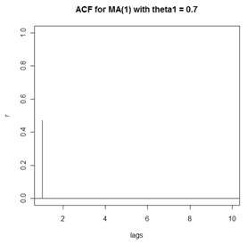
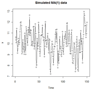
The plot just shown is the theoretical ACF for an MA(1) with \(\theta_1=0.7\). In practice, a sample won’t usually provide such a clear pattern. Using R, we simulated n = 100 sample values using the model \(x_t=10+w_t+.7w_{t-1}\) where \(w_t \overset{iid}{\sim} N(0,1)\). For this simulation, a time series plot of the sample data follows. We can’t tell much from this plot.
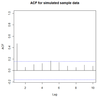
The sample ACF for the simulated data follows. We see a “spike” at lag 1 followed by generally non-significant values for lags past 1. Note that the sample ACF does not exactly match the theoretical pattern of the underlying MA(1), which is that all autocorrelations for lags above lag 1 equal zero. A different sample would have a slightly different sample ACF shown below, but would likely have the same broad features.
Theoretical Properties of a Time Series with an MA(2) Model
For the MA(2) model, theoretical properties are the following:
- Mean is \(E(x_t)=\mu\)
- Variance is \(Var(x_t)=\sigma^2_w(1+\theta^2_1+\theta^2_2)\)
- Autocorrelation function (ACF) is:
\( \rho_1 = \dfrac{\theta_1+\theta_1\theta_2}{1+\theta^2_1 +\theta^2_2}, \text{ } \rho_2 = \dfrac{\theta_2}{1+\theta^2_1 +\theta^2_2}, \text{ and } \rho_h = 0 \text{ for } h \ge 3 \)
The only nonzero values in the theoretical ACF are for lags 1 and 2. Autocorrelations for higher lags are 0. So, a sample ACF with significant autocorrelations at lags 1 and 2, but non-significant autocorrelations for higher lags indicates a possible MA(2) model.
Example 2-2
Consider the MA(2) model \(x_t=10+w_t+.5w_{t-1}+.3w_{t-2}\), where \(w_t \overset{iid}{\sim} N(0,1)\). The coefficients are \(\theta_1=0.5\) and \(\theta_2= 0.3\). Because this is an MA(2), the theoretical ACF will have nonzero values only at lags 1 and 2.
Values of the two nonzero autocorrelations are:
\(\rho_1 = \dfrac{0.5+0.5 \times 0.3}{1+0.5^2 +0.3^2} = 0.4851 \text{ and } \rho_2 = \dfrac{0.3}{1+0.5^2 +0.3^2}= 0.2239 \)
A plot of the theoretical ACF follows:
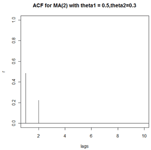
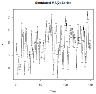
As nearly always is the case, sample data won’t behave quite so perfectly as theory. We simulated n = 150 sample values for the model \(x_t=10+w_t+.5w_{t-1}+.3w_{t-2}\), where \(w_t \overset{iid}{\sim} N(0,1)\). The time series plot of the data follows. As with the time series plot for the MA(1) sample data, you can’t tell much from it.
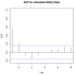
The sample ACF for the simulated data follows. The pattern is typical for situations where an MA(2) model may be useful. There are two statistically significant “spikes” at lags 1 and 2 followed by non-significant values for other lags. Note that due to sampling error, the sample ACF did not match the theoretical pattern exactly.
ACF for General MA(q) Models
A property of MA(q) models in general is that there are nonzero autocorrelations for the first q lags and autocorrelations = 0 for all lags > q.
Non-uniqueness of connection between values of \(\theta_1\) and \(\rho_1\) in MA(1) Model.
In the MA(1) model, for any value of \(\theta_1\), the reciprocal \(1/\theta_1\) gives the same value for:
\(\rho_1 = \dfrac{\theta_1}{1+\theta^2_1}\)
As an example, use +0.5 for \(\theta_1\), and then use 1/(0.5) = 2 for \(\theta_1\). You’ll get \(\rho_1 = 0.4\) in both instances.
To satisfy a theoretical restriction called invertibility, we restrict MA(1) models to have values with absolute value less than 1. In the example just given, \(\theta_1 = 0.5\) will be an allowable parameter value, whereas \(\theta_1 = 1/0.5 = 2\) will not.
Invertibility of MA models
An MA model is said to be invertible if it is algebraically equivalent to a converging infinite order AR model. By converging, we mean that the AR coefficients decrease to 0 as we move back in time.
Invertibility is a restriction programmed into time series software used to estimate the coefficients of models with MA terms. It’s not something that we check for in the data analysis. Additional information about the invertibility restriction for MA(1) models is given in the appendix.
For a MA(q) model with a specified ACF, there is only one invertible model. The necessary condition for invertibility is that the \(\theta\) coefficients have values such that the equation \(1-\theta_1y-...-\theta_qy^q=0\) has solutions for \(y\) that fall outside the unit circle.
R
R Code for the Examples
In Example 1, we plotted the theoretical ACF of the model \(x_t=10+w_t+.7w_{t-1}\), and then simulated n = 150 values from this model and plotted the sample time series and the sample ACF for the simulated data. The R commands used to plot the theoretical ACF were:
acfma1=ARMAacf(ma=c(0.7), lag.max=10) # 10 lags of ACF for MA(1) with theta1 = 0.7
lags=0:10 #creates a variable named lags that ranges from 0 to 10.
plot(lags,acfma1,xlim=c(1,10), ylab="r",type="h", main = "ACF for MA(1) with theta1 = 0.7")
abline(h=0) #adds a horizontal axis to the plot
The first command determines the ACF and stores it in an object named acfma1 (our choice of name).
The plot command (the 3rd command) plots lags versus the ACF values for lags 1 to 10. The ylab parameter labels the y-axis and the "main" parameter puts a title on the plot.
To see the numerical values of the ACF simply use the command acfma1.
The simulation and plots were done with the following commands:
xc=arima.sim(n=150, list(ma=c(0.7))) #Simulates n = 150 values from MA(1)
x=xc+10 # adds 10 to make mean = 10. Simulation defaults to mean = 0.
plot(x,type="b", main="Simulated MA(1) data")
acf(x, xlim=c(1,10), main="ACF for simulated sample data")
In Example 2, we plotted the theoretical ACF of the model \(x_t=10+w_t+.5w_{t-1}+.3w_{t-2}\), and then simulated n = 150 values from this model and plotted the sample time series and the sample ACF for the simulated data. The R commands used were:
acfma2=ARMAacf(ma=c(0.5,0.3), lag.max=10)
acfma2
lags=0:10
plot(lags,acfma2,xlim=c(1,10), ylab="r",type="h", main = "ACF for MA(2) with theta1 = 0.5,theta2=0.3")
abline(h=0)
xc=arima.sim(n=150, list(ma=c(0.5, 0.3)))
x=xc+10
plot(x, type="b", main = "Simulated MA(2) Series")
acf(x, xlim=c(1,10), main="ACF for simulated MA(2) Data")
Appendix: Proof of Properties of MA(1)
For interested students, here are proofs for theoretical properties of the MA(1) model.
The 1st order moving average model , denoted by MA(1) is \(x_t=\mu+w_t+\theta_1w_{t-1}\), where \(w_t \overset{iid}{\sim} N(0,\sigma^2_w)\).
Mean: \( E(x_t)=E(\mu + w_t + \theta_1 w_{t-1} ) = \mu + 0 + (\theta_1)(0) = \mu \)
Variance: \(\text{Var}(x_t) = \text{Var} (\mu + w_t + \theta_1 w_{t-1}) = 0 + \text{Var}(w_t) + \text{Var}(\theta_1w_{t-1}) = \sigma^2_w + \theta^2_1\sigma^2_w = (1+\theta^2_1)\sigma^2_w\)
ACF: Consider the covariance between \(x_t\) and \(x_{t-h}\). This is \(E(x_t-\mu)(x_{t-h}-\mu)\), which equals
\(E[(w_t + \theta_1w_{t-1})(w_{t-h}+\theta_1w_{t-h-1})] = E[w_tw_{t-h} + \theta_1w_{t-1}w_{t-h} +\theta_1w_tw_{t-h-1}+\theta^2_1 w_{t-1}w_{t-h-1}]\)
When \(h=1\), the previous expression = \(\theta_1 \sigma_w^2\). For any \(h \ge 2\), the previous expression = 0. The reason is that, by definition of independence of the \(w_t\), \(E(w_k w_k)=0\) for any \(k \ne j \). Further, because the \(w_t\) have mean 0, \(E(w_k w_k)=E(w_j^2)=\sigma_w^2\).
For a time series,
\(\rho_h = \dfrac{\text{Covariance for lag h}}{\text{Variance}}\)
Apply this result to get the ACF given above.
Invertibility Restriction:
An invertible MA model is one that can be written as an infinite order AR model that converges so that the AR coefficients converge to 0 as we move infinitely back in time. We’ll demonstrate invertibility for the MA(1) model.
The MA(1) model can be written as \(x_t-\mu=w_t+\theta_1 w_{t-1}\).
If we let \(z_t=x_t-\mu\), then the MA(1) model is
(1) \(z_t = w_t +\theta_1w_{t-1}\).
At time \(t-1\), the model is \(z_{t-1}=w_{t-1}+\theta_1 w_{t-2}\) which can be reshuffled to
(2) \(w_{t-1} = z_{t-1}-\theta_1w_{t-2}\).
We then substitute relationship (2) for \(w_{t-1}\) in equation (1)
(3) \(z_t = w_t +\theta_1(z_{t-1}-\theta_1w_{t-2}) = w_t +\theta_1z_{t-1} -\theta^2w_{t-2}\)
At time \(t-2\), equation (2) becomes
(4) \(w_{t-2} = z_{t-2}-\theta_1w_{t-3}\).
We then substitute relationship (4) for \(w_{t-2}\) in equation (3)
\(z_t = w_t +\theta_1 z_{t-1}-\theta^2_1w_{t-2} = w_t + \theta_1z_{t-1} -\theta^2_1(z_{t-2}-\theta_1w_{t-3}) = w_t +\theta_1z_{t-1} -\theta_1^2z_{t-2}+\theta^3_1w_{t-3}\)
If we were to continue (infinitely), we would get the infinite order AR model
\(z_t = w_t +\theta_1 z_{t-1} - \theta^2_1z_{t-2} +\theta^3_1z_{t-3}-\theta^4_1z_{t-4}+\dots \)
However, that if \(\lvert\theta_1\rvert \ge 1\), the coefficients multiplying the lags of \(z\) will increase (infinitely) in size as we move back in time. To prevent this, we need \(\lvert\theta_1\rvert < 1\). This is the condition for an invertible MA(1) model.
Infinite Order MA model
In week 3, we’ll see that an AR(1) model can be converted to an infinite order MA model:
\(x_t -\mu = w_t +\phi_1w_{t-1}+\phi^2_1w_{t-2} + \dots + \phi^k_1 w_{t-k} +\dots = \sum_{j=0}^{\infty} \phi^j_1w_{t-j}\)
This summation of past white noise terms is known as the causal representation of an AR(1). In other words, \(x_t\) is a special type of MA with an infinite number of terms going back in time. This is called an infinite order MA or MA(\(\infty \)). A finite order MA is an infinite order AR and any finite order AR is an infinite order MA.
Recall in Week 1, we noted that a requirement for a stationary AR(1) is that \(\lvert\phi_1\rvert< 1\). Let’s calculate the \(\text{Var}(x_t)\) using the causal representation.
\(\text{Var}(x_t) = \text{Var} \left(\sum_{j=0}^{\infty} \phi^j_1w_{t-j} = \sum_{j=0}^{\infty}\text{Var}(\phi^j_1w_{t-j}) = \sum_{j=0}^{\infty}\phi^{2j}_1\sigma^2_w = \sigma^2_w \sum_{j=0}^{\infty}\phi^{2j}_1 = \frac{\sigma^2_w}{1-\phi^2_1} \right)\)
This last step uses a basic fact about geometric series that requires \(\lvert\phi_1\rvert <1\); otherwise the series diverges.
2.2 Partial Autocorrelation Function (PACF)
2.2 Partial Autocorrelation Function (PACF)In general, a partial correlation is a conditional correlation. It is the correlation between two variables under the assumption that we know and take into account the values of some other set of variables. For instance, consider a regression context in which y is the response variable and \(x_1\), \(x_2\), and \(x_3\) are predictor variables. The partial correlation between y and \(x_3\) is the correlation between the variables determined taking into account how both y and \(x_3\) are related to \(x_1\) and \(x_2\).
In regression, this partial correlation could be found by correlating the residuals from two different regressions:
- Regression in which we predict y from \(x_1\) and \(x_2\),
- regression in which we predict \(x_3\) from \(x_1\) and \(x_2\). Basically, we correlate the “parts” of y and \(x_3\) that are not predicted by \(x_1\) and \(x_2\).
More formally, we can define the partial correlation just described as
\(\dfrac{\text{Covariance}(y, x_3|x_1, x_2)}{\sqrt{\text{Variance}(y|x_1, x_2)\text{Variance}(x_3| x_1, x_2)}}\)
That this is also how the parameters of a regression model are interpreted. Think about the difference between interpreting the regression models:
\(y = \beta_0 + \beta_1x^2 \text{ and } y = \beta_0+\beta_1x+\beta_2x^2\)
In the first model, \(\beta_1\) can be interpreted as the linear dependency between \(x^2\) and y. In the second model, \(\beta_2\) would be interpreted as the linear dependency between \(x^2\) and y WITH the dependency between x and y already accounted for.
For a time series, the partial autocorrelation between \(x_{t}\) and \(x_{t-h}\) is defined as the conditional correlation between \(x_{t}\) and \(x_{t-h}\), conditional on \(x_{t-h+1}\), ... , \(x_{t-1}\), the set of observations that come between the time points \(t\) and \(t-h\).
- The 1st order partial autocorrelation will be defined to equal the 1st order autocorrelation.
- The 2nd order (lag) partial autocorrelation is
\(\dfrac{\text{Covariance}(x_t, x_{t-2}| x_{t-1})}{\sqrt{\text{Variance}(x_t|x_{t-1})\text{Variance}(x_{t-2}|x_{t-1})}}\)
This is the correlation between values two time periods apart conditional on knowledge of the value in between. (By the way, the two variances in the denominator will equal each other in a stationary series.)
- The 3rd order (lag) partial autocorrelation is
\(\dfrac{\text{Covariance}(x_t, x_{t-3}| x_{t-1}, x_{t-2})}{\sqrt{\text{Variance}(x_t|x_{t-1},x_{t-2})\text{Variance}(x_{t-3}|x_{t-1},x_{t-2})}}\)
And, so on, for any lag.
Typically, matrix manipulations having to do with the covariance matrix of a multivariate distribution are used to determine estimates of the partial autocorrelations.
Some Useful Facts About PACF and ACF Patterns
Identification of an AR model is often best done with the PACF.
- For an AR model, the theoretical PACF “shuts off” past the order of the model. The phrase “shuts off” means that in theory the partial autocorrelations are equal to 0 beyond that point. Put another way, the number of non-zero partial autocorrelations gives the order of the AR model. By the “order of the model” we mean the most extreme lag of x that is used as a predictor.
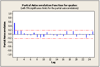
Example: In Lesson 1.2, we identified an AR(1) model for a time series of annual numbers of worldwide earthquakes having a seismic magnitude greater than 7.0. Following is the sample PACF for this series. Note that the first lag value is statistically significant, whereas partial autocorrelations for all other lags are not statistically significant. This suggests a possible AR(1) model for these data.
Identification of an MA model is often best done with the ACF rather than the PACF.
For an MA model, the theoretical PACF does not shut off, but instead tapers toward 0 in some manner. A clearer pattern for an MA model is in the ACF. The ACF will have non-zero autocorrelations only at lags involved in the model.
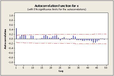
Lesson 2.1 included the following sample ACF for a simulated MA(1) series. Note that the first lag autocorrelation is statistically significant whereas all subsequent autocorrelations are not. This suggests a possible MA(1) model for the data.
The model used for the simulation was \(x_t=10+w_t+0.7w_{t-1}\). In theory, the first lag autocorrelation \(\theta_1 / (1+\theta_1^2) = .7/(1+.7^2) = .4698 \) and autocorrelations for all other lags = 0.
The underlying model used for the MA(1) simulation in Lesson 2.1 was \(x_t=10+w_t+0.7w_{t-1}\). Following is the theoretical PACF (partial autocorrelation) for that model. Note that the pattern gradually tapers to 0.
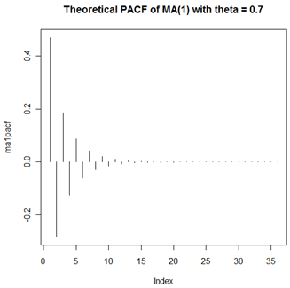
The PACF just shown was created in R with these two commands:
ma1pacf = ARMAacf(ma = c(.7),lag.max = 36, pacf=TRUE)
plot(ma1pacf,type="h", main = "Theoretical PACF of MA(1) with theta = 0.7")
2.3 Notational Conventions
2.3 Notational ConventionsTime series models (in the time domain) involve lagged terms and may involve differenced data to account for trend. There are useful notations used for each.
Backshift Operator
Using B before either a value of the series \(x_t\) or an error term wt means to move that element back one time. For instance,
\(Bx_t = x_{t-1}\)
A “power” of B means to repeatedly apply the backshift in order to move back a number of time periods that equals the “power.” As an example,
\(B^2 x_t = x_{t-2}\)
\( x_{t-2}\) represents \(x_t\) two units back in time. \(B^k x_t = x_{t-k}\) represents \(x_t\) k units back in time. The backshift operator B doesn't operate on coefficients because they are fixed quantities that do not move in time. For example, \(B\theta_1=\theta_1\).
AR Models and the AR Polynomial
AR models can be written compactly using an "AR polynomial" involving coefficients and backshift operators. Let p = the maximum order (lag) of the AR terms in the model. The general form for an AR polynomial is
\(\Phi(B) = 1-\phi_1B- \dots - \phi_p B^p\)
Using the AR polynomial one way to write an AR model is
\(\Phi(B)x_t = \delta + w_t\)
Examples 2-3
Consider the AR(1) model \(x_t=\delta+\phi_1x_{t-1}+w_t\) where \(w_t \overset{iid}{\sim} N(0,\sigma_w^2)\). For an AR(1), the maximum lag = 1 so the AR polynomial is
\(\Phi(B) = 1-\phi_1B\)
and the model can be written
\((1-\phi_1B)x_t = \delta + w_t\)
To check that this works, we can multiply out the left side to get
\(x_t - \phi_1x_{t-1} = \delta +w_t\)
Then, swing the \(-\phi_1x_{t-1}\) over to the right side and we get
\(x_t = \delta + \phi_1x_{t-1}+w_t\)
An AR(2) model is \(x_t = \delta + \phi_1x_{t-1}+\phi_2x_{t-2}+w_t\). That is, xt is a linear function of the values of x at the previous two lags. The AR polynomial for an AR(2) model is
\(\Phi(B) = 1-\phi_1B-\phi_2B^2\)
The AR(2) model could be written as \(( 1-\phi_1B-\phi_2B^2) x_t = \delta + w_t\), or as \(\Phi(B)x_t = \delta + w_t\) with an additional explanation that \(\Phi(B) = 1-\phi_1B-\phi_2B^2\)
An AR(p) model is \(x_t = \delta + \phi_1x_{t-1}+\phi_2x_{t-2}+ ... + \phi_p x_{t-p} + w_t\), where \(\phi_1, \phi_2, ..., \phi_p\) are constants and may be greater than 1. (Recall that \( |\phi_1| < 1 \) for an AR(1) model.) Here xt is a linear function of the values of x at the previous p lags.
A shorthand notation for the AR polynomial is \(\Phi(B)\) and a general AR model might be written as \(\Phi(B)x_t = \delta + w_t\). Of course, you would have to specify the order of the model somewhere on the side.
MA Models
A MA(1) model \(x_t = \mu + w_t + \theta_1 w_{t-1}\) could be written as \(x_t = \mu + (1+\theta_1B)w_t\). A factor such as \(1+\theta_1B\) is called the MA polynomial, and it is denoted as \(\Theta(B)\).
A MA(2) model is defined as \(x_t = \mu + w_t + \theta_1 w_{t-1} + \theta_2 w_{t-2}\) and could be written as \(x_t = \mu + (1+\theta_1B+\theta_2B^2)w_t\). Here, the MA polynomial is \(\Theta(B) = (1+\theta_1B+\theta_2B^2)\).
In general, the MA polynomial is \(\Theta(B) = (1+\theta_1B+\dots +\theta_qB^q)\), where \(q\) = maximum order (lag) for MA terms in the model.
In general, we can write an MA model as \(x_t - \mu = \Theta(B)w_t\).
Models with Both AR and MA Terms
A model that involves both AR and MA terms might be written \(\Phi(B)(x_t-\mu) = \Theta(B)w_t\) or possibly even
\((x_t-\mu) = \dfrac{\Theta(B)}{\Phi(B)}w_t\)
Many textbooks and software programs define the MA polynomial with negative signs rather than positive signs as above. This doesn’t change the properties of the model, or with a sample, the overall fit of the model. It only changes the algebraic signs of the MA coefficients. Always check to see how your software is defining the MA polynomial. For example is the MA(1) polynomial \(1+\theta_1B\) or \(1-\theta_1B\)?
Differencing
Often differencing is used to account for nonstationarity that occurs in the form of trend and/or seasonality.
The difference \(x _ { t } - x _ { t - 1 }\) can be expressed as \( \left( 1 - B \right)_{ X _ { t } } \).
An alternative notation for a difference is
\(\nabla = 1-B\)
Thus
\(\nabla x_t = (1-B)x_t = x_t-x_{t-1}\)
A subscript defines a difference of a lag equal to the subscript. For instance,
\(\nabla_{12}x_t = x_t - x_{t-12}\)
This type of difference is often used with monthly data that exhibits seasonality. The idea is that differences from the previous year may be, on average, about the same for each month of a year.
A superscript says to repeat the differencing the specified number of times. As an example,
\(\nabla^2 x_t = (1-B)^2x_t = (1-2B+B^2)x_t = x_t -2x_{t-1}+x_{t-2}\)
In words, this is a first difference of the first differences.