Time Series Analysis is a way of studying the characteristics of the response variable concerning time as the independent variable. To estimate the target variable in predicting or forecasting, use the time variable as the reference point. TSA represents a series of time-based orders, it would be Years, Months, Weeks, Days, Horus, Minutes, and Seconds. It is an observation from the sequence of discrete time of successive intervals. Some real-world application of TSA includes weather forecasting models, stock market predictions, signal processing, and control systems. Since TSA involves producing the set of information in a particular sequence, this makes it distinct from spatial and other analyses. We could predict the future using AR, MA, ARMA, and ARIMA models. In this article, we will be decoding time series analysis for you.
In this article, you will explore time series analysis, uncovering what time series analysis is and how it applies to time series forecasting. We will delve into various time series models and their significance in machine learning, providing insights into effective time series forecasting techniques. Join us as we navigate about the time series analysis in machine learning!
Learning Objectives
- We will discuss in detail TSA Objectives, Assumptions, and Components (stationary and non-stationary).
- We will look at the TSA algorithms.
- Finally, we will look at specific use cases in Python.
This article was published as a part of the Data Science Blogathon.
Table of contents
- What is Time Series Analysis?
- How to Analyze Time Series?
- Significance of Time Series
- Components of Time Series Analysis
- Limitations of Time Series Analysis?
- Data Types of Time Series
- Methods to Check Stationarity
- Converting Non-Stationary Into Stationary
- Moving Average Methodology
- Time Series Analysis in Data Science and Machine Learning
- What is an Auto-Regressive Model?
- Implementation of Auto-Regressive Model
- Implementation of Moving Average (Weights – Simple Moving Average)
- Understanding ARMA and ARIMA
- Understand the signature of ARIMA
- Process Flow (Re-Gap)
- Conclusion
What is Time Series Analysis?
Time series analysis is a statistical technique used to analyze data points gathered at consistent intervals over a time span in order to detect patterns and trends. Understanding the fundamental framework of the data can assist in predicting future data points and making knowledgeable choices.
Objectives of Time Series Analysis
- To understand how time series works and what factors affect a certain variable(s) at different points in time.
- Time series analysis will provide the consequences and insights of the given dataset’s features that change over time.
- Supporting to derive the predicting the future values of the time series variable.
- Assumptions: There is only one assumption in TSA, which is “stationary,” which means that the origin of time does not affect the properties of the process under the statistical factor.
How to Analyze Time Series?
To perform the time series analysis, we have to follow the following steps:
- Collecting the data and cleaning it
- Preparing Visualization with respect to time vs key feature
- Observing the stationarity of the series
- Developing charts to understand its nature.
- Model building – AR, MA, ARMA and ARIMA
- Extracting insights from prediction
Significance of Time Series
TSA is the backbone for prediction and forecasting analysis, specific to time-based problem statements.
- Analyzing the historical dataset and its patterns
- Understanding and matching the current situation with patterns derived from the previous stage.
- Understanding the factor or factors influencing certain variable(s) in different periods.
With the help of “Time Series,” we can prepare numerous time-based analyses and results.
- Forecasting: Predicting any value for the future.
- Segmentation: Grouping similar items together.
- Classification: Classifying a set of items into given classes.
- Descriptive analysis: Analysis of a given dataset to find out what is there in it.
- Intervention analysis: Effect of changing a given variable on the outcome.
Components of Time Series Analysis
Let’s look at the various components of Time Series Analysis:
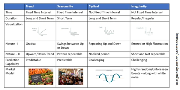
- Trend: In which there is no fixed interval and any divergence within the given dataset is a continuous timeline. The trend would be Negative or Positive or Null Trend
- Seasonality: In which regular or fixed interval shifts within the dataset in a continuous timeline. Would be bell curve or saw tooth
- Cyclical: In which there is no fixed interval, uncertainty in movement and its pattern
- Irregularity: Unexpected situations/events/scenarios and spikes in a short time span.
Limitations of Time Series Analysis?
Time series has the below-mentioned limitations; we have to take care of those during our data analysis.
- Similar to other models, the missing values are not supported by TSA
- The data points must be linear in their relationship.
- Data transformations are mandatory, so they are a little expensive.
- Models mostly work on Uni-variate data.
Data Types of Time Series
Let’s discuss the time series’ data types and their influence. While discussing TS data types, there are two major types – stationary and non-stationary.
Stationary: A dataset should follow the below thumb rules without having Trend, Seasonality, Cyclical, and Irregularity components of the time series.
- The mean value of them should be completely constant in the data during the analysis.
- The variance should be constant with respect to the time-frame
- Covariance measures the relationship between two variables.
Non- Stationary: If either the mean-variance or covariance is changing with respect to time, the dataset is called non-stationary.
Methods to Check Stationarity
During the TSA model preparation workflow, we must assess whether the dataset is stationary or not. This is done using Statistical Tests. There are two tests available to test if the dataset is stationary:
- Augmented Dickey-Fuller (ADF) Test
- Kwiatkowski-Phillips-Schmidt-Shin (KPSS) Test
Augmented Dickey-Fuller (ADF) Test or Unit Root Test
The ADF test is the most popular statistical test. It is done with the following assumptions:
- Null Hypothesis (H0): Series is non-stationary
- Alternate Hypothesis (HA): Series is stationary
- p-value >0.05 Fail to reject (H0)
- p-value <= 0.05 Accept (H1)
Kwiatkowski–Phillips–Schmidt–Shin (KPSS) Test
These tests assess a NULL Hypothesis (HO), perceiving the time series as stationary around a deterministic trend, in contrast to the alternative of a unit root. Since TSA is looking for Stationary Data for its further analysis, we have to ensure that the dataset is stationary.
Converting Non-Stationary Into Stationary
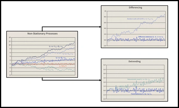
Let’s discuss quickly how to convert non-stationary to stationary for effective time series modeling. There are three methods available for this conversion – detrending, differencing, and transformation.
Detrending
It involves removing the trend effects from the given dataset and showing only the differences in values from the trend. It always allows cyclical patterns to be identified.

Differencing
This is a simple transformation of the series into a new time series, which we use to remove the series dependence on time and stabilize the mean of the time series, so trend and seasonality are reduced during this transformation.
- Yt= Yt – Yt-1
- Yt=Value with time
Transformation
This includes three different methods they are Power Transform, Square Root, and Log Transfer. The most commonly used one is Log Transfer.
Moving Average Methodology
The commonly used time series method is the Moving Average. This method is slick with random short-term variations. Relatively associated with the components of time series.
The Moving Average (MA) (or) Rolling Mean: The value of MA is calculated by taking average data of the time-series within k periods.
Let’s see the types of moving averages:
- Simple Moving Average (SMA),
- Cumulative Moving Average (CMA)
- Exponential Moving Average (EMA)
Simple Moving Average (SMA)
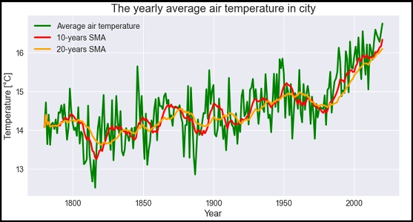
The Simple Moving Average (SMA) calculates the unweighted mean of the previous M or N points. We prefer selecting sliding window data points based on the amount of smoothing, as increasing the value of M or N improves smoothing but reduces accuracy.
To understand better, I will use the air temperature dataset.

Code
import pandas as pd
from matplotlib import pyplot as plt
from statsmodels.graphics.tsaplots import plot_acf
df_temperature = pd.read_csv('temperature_TSA.csv', encoding='utf-8')
df_temperature.head()
Output

Code
df_temperature.info()Output

Code
# set index for year column
df_temperature.set_index('Any', inplace=True)
df_temperature.index.name = 'year'
# Yearly average air temperature - calculation
df_temperature['average_temperature'] = df_temperature.mean(axis=1)
# drop unwanted columns and resetting the datafreame
df_temperature = df_temperature[['average_temperature']]
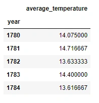
df_temperature.head()
Output
Code
# SMA over a period of 10 and 20 years
df_temperature['SMA_10'] = df_temperature.average_temperature.rolling(10, min_periods=1).mean()
df_temperature['SMA_20'] = df_temperature.average_temperature.rolling(20, min_periods=1).mean()

# Grean = Avg Air Temp, RED = 10 yrs, ORANG colors for the line plot
colors = ['green', 'red', 'orange']
# Line plot
df_temperature.plot(color=colors, linewidth=3, figsize=(12,6))
plt.xticks(fontsize=14)
plt.yticks(fontsize=14)
plt.legend(labels =['Average air temperature', '10-years SMA', '20-years SMA'], fontsize=14)
plt.title('The yearly average air temperature in city', fontsize=20)
plt.xlabel('Year', fontsize=16)
plt.ylabel('Temperature [°C]', fontsize=16)
Output
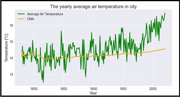
Cumulative Moving Average (CMA)
The CMA is the unweighted mean of past values till the current time.

Code
# CMA Air temperature
df_temperature['CMA'] = df_temperature.average_temperature.expanding().mean()

# green -Avg Air Temp and Orange -CMA
colors = ['green', 'orange']
# line plot
df_temperature[['average_temperature', 'CMA']].plot(color=colors, linewidth=3, figsize=(12,6))
plt.xticks(fontsize=14)
plt.yticks(fontsize=14)
plt.legend(labels =['Average Air Temperature', 'CMA'], fontsize=14)
plt.title('The yearly average air temperature in city', fontsize=20)
plt.xlabel('Year', fontsize=16)
plt.ylabel('Temperature [°C]', fontsize=16)
Output
Exponential Moving Average (EMA)
EMA is mainly used to identify trends and filter out noise. The weight of elements is decreased gradually over time. This means It gives weight to recent data points, not historical ones. Compared with SMA, the EMA is faster to change and more sensitive.
α –>Smoothing Factor.
- It has a value between 0,1.
- Represents the weighting applied to the very recent period.
Let’s apply the exponential moving averages with a smoothing factor of 0.1 and 0.3 in the given dataset.

Code
# EMA Air Temperature
# Let's smoothing factor - 0.1
df_temperature['EMA_0.1'] = df_temperature.average_temperature.ewm(alpha=0.1, adjust=False).mean()
# Let's smoothing factor  - 0.3
df_temperature['EMA_0.3'] = df_temperature.average_temperature.ewm(alpha=0.3, adjust=False).mean()

# green - Avg Air Temp, red- smoothing factor - 0.1, yellow - smoothing factor  - 0.3
colors = ['green', 'red', 'yellow']
df_temperature[['average_temperature', 'EMA_0.1', 'EMA_0.3']].plot(color=colors, linewidth=3, figsize=(12,6), alpha=0.8)
plt.xticks(fontsize=14)
plt.yticks(fontsize=14)
plt.legend(labels=['Average air temperature', 'EMA - alpha=0.1', 'EMA - alpha=0.3'], fontsize=14)
plt.title('The yearly average air temperature in city', fontsize=20)
plt.xlabel('Year', fontsize=16)
plt.ylabel('Temperature [°C]', fontsize=16)
Output

Time Series Analysis in Data Science and Machine Learning
When dealing with TSA in Data Science and Machine Learning, there are multiple model options are available. In which the Autoregressive–Moving-Average (ARMA) models with [p, d, and q].
- P==> autoregressive lags
- q== moving average lags
- d==> difference in the order
Before we get to know about Arima, first, you should understand the below terms better.
- Auto-Correlation Function (ACF)
- Partial Auto-Correlation Function (PACF)
Auto-Correlation Function (ACF)
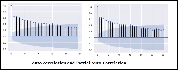
ACF indicates how similar a value is within a given time series and the previous value. (OR) It measures the degree of the similarity between a given time series and the lagged version of that time series at the various intervals we observed.
Python Statsmodels library calculates autocorrelation. It identifies a set of trends in the given dataset and the influence of former observed values on the currently observed values.
Partial Auto-Correlation (PACF)
PACF is similar to Auto-Correlation Function and is a little challenging to understand. It always shows the correlation of the sequence with itself with some number of time units per sequence order in which only the direct effect has been shown, and all other intermediary effects are removed from the given time series.
Auto-Correlation and Partial Auto-Correlation
Code
plot_acf(df_temperature)
plt.show()

plot_acf(df_temperature, lags=30)
plt.show()
Output
Observation
The previous temperature influences the current temperature, but the significance of that influence decreases and slightly increases from the above visualization along with the temperature with regular time intervals.
Types of Auto-Correlation

Interpret ACF and PACF Plots
| ACF | PACF | Perfect ML -Model |
| Plot declines gradually | Plot drops instantly | Auto Regressive model. |
| Plot drops instantly | Plot declines gradually | Moving Average model |
| Plot decline gradually | Plot Decline gradually | ARMA |
| Plot drop instantly | Plot drop instantly | You wouldn’t perform any model |
Remember that both ACF and PACF require stationary time series for analysis.
What is an Auto-Regressive Model?
An auto-regressive model is a simple model that predicts future performance based on past performance. It is mainly used for forecasting when there is some correlation between values in a given time series and those that precede and succeed (back and forth).
An AR is a Linear Regression model that uses lagged variables as input. By indicating the input, the Linear Regression model can be easily built using the scikit-learn library. Statsmodels library provides autoregression model-specific functions where you must specify an appropriate lag value and train the model. It is provided in the AutoTeg class to get the results using simple steps.
- Creating the model AutoReg()
- Call fit() to train it on our dataset.
- Returns an AutoRegResults object.
- Once fit, make a prediction by calling the predict () function
The equation for the AR model (Let’s compare Y=mX+c)
Yt =C+b1 Yt-1+ b2 Yt-2+……+ bp Yt-p+ Ert
Key Parameters
- p=past values
- Yt=Function of different past values
- Ert=errors in time
- C=intercept
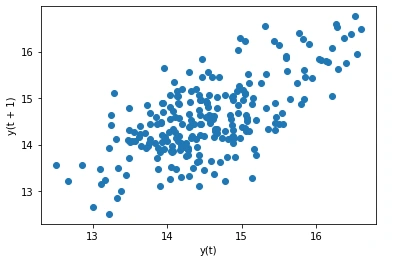
Lets’s check whether the given data set or time series is random or not.
Code
from matplotlib import pyplot
from pandas.plotting import lag_plot
lag_plot(df_temperature)
pyplot.show()
Output
Observation
Yes, it looks random and scattered.
Implementation of Auto-Regressive Model
Code
#import libraries
from matplotlib import pyplot
from statsmodels.tsa.ar_model import AutoReg
from sklearn.metrics import mean_squared_error
from math import sqrt
# load csv as dataset
#series = read_csv('daily-min-temperatures.csv', header=0, index_col=0, parse_dates=True, squeeze=True)
# split dataset for test and training
X = df_temperature.values
train, test = X[1:len(X)-7], X[len(X)-7:]
# train autoregression
model = AutoReg(train, lags=20)
model_fit = model.fit()
print('Coefficients: %s' % model_fit.params)
# Predictions
predictions = model_fit.predict(start=len(train), end=len(train)+len(test)-1, dynamic=False)
for i in range(len(predictions)):
    print('predicted=%f, expected=%f' % (predictions[i], test[i]))
rmse = sqrt(mean_squared_error(test, predictions))
print('Test RMSE: %.3f' % rmse)
# plot results
pyplot.plot(test)
pyplot.plot(predictions, color='red')
pyplot.show()
Output
predicted=15.893972, expected=16.275000
predicted=15.917959, expected=16.600000
predicted=15.812741, expected=16.475000
predicted=15.787555, expected=16.375000
predicted=16.023780, expected=16.283333
predicted=15.940271, expected=16.525000
predicted=15.831538, expected=16.758333
Test RMSE: 0.617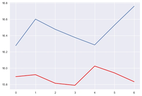
Observation
Expected (blue) Against Predicted (red). The forecast looks good on the 4th and the deviation on the 6th day.
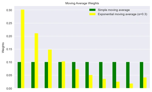
Implementation of Moving Average (Weights – Simple Moving Average)
Code
import numpy as np
alpha= 0.3
n = 10
w_sma = np.repeat(1/n, n)
colors = ['green', 'yellow']
# weights - exponential moving average alpha=0.3 adjust=False
w_ema = [(1-ALPHA)**i if i==N-1 else alpha*(1-alpha)**i for i in range(n)]
pd.DataFrame({'w_sma': w_sma, 'w_ema': w_ema}).plot(color=colors, kind='bar', figsize=(8,5))
plt.xticks([])
plt.yticks(fontsize=10)
plt.legend(labels=['Simple moving average', 'Exponential moving average (α=0.3)'], fontsize=10)
# title and labels
plt.title('Moving Average Weights', fontsize=10)
plt.ylabel('Weights', fontsize=10)
Output
Understanding ARMA and ARIMA
ARMA is a combination of the Auto-Regressive and Moving Average models for forecasting. This model provides a weakly stationary stochastic process in terms of two polynomials, one for the Auto-Regressive and the second for the Moving Average.
ARMA is best for predicting stationary series. ARIMA was thus developed to support both stationary as well as non-stationary series.

- AR ==> Uses past values to predict the future.
- MA ==> Uses past error terms in the given series to predict the future.
- I==> Uses the differencing of observation and makes the stationary data.
AR+I+MA= ARIMA
Understand the signature of ARIMA
- p==> log order => No of lag observations.
- d==> degree of differencing => No of times that the raw observations are differenced.
- q==>order of moving average => the size of the moving average window
Implementation Steps for ARIMA
- Plot a time series format
- Difference to make stationary on mean by removing the trend
- Make stationary by applying log transform.
- Difference log transform to make as stationary on both statistic mean and variance
- Plot ACF & PACF, and identify the potential AR and MA model
- Discovery of best fit ARIMA model
- Forecast/Predict the value using the best fit ARIMA model
- Plot ACF & PACF for residuals of the ARIMA model, and ensure no more information is left.
Implementation of ARIMA in Python
We have already discussed steps 1-5 which will remain the same; let’s focus on the rest here.
Code
from statsmodels.tsa.arima_model import ARIMA
model = ARIMA(df_temperature, order=(0, 1, 1))
results_ARIMA = model.fit()

results_ARIMA.summary()
Output

Code
results_ARIMA.forecast(3)[0]Output
array([16.47648941, 16.48621826, 16.49594711])Code
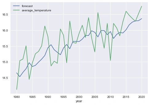
results_ARIMA.plot_predict(start=200)
plt.show()
Output
Process Flow (Re-Gap)

In recent years, the use of Deep Learning for Time Series Analysis and Forecasting has increased to resolve problem statements that couldn’t be handled using Machine Learning techniques. Let’s discuss this briefly.

Recurrent Neural Networks (RNN) is the most traditional and accepted architecture fitment for Time-Series forecasting-based problems.
RNN is organized into successive layers and divided into
- Input
- Hidden
- Output
Each layer has equal weight, and every neuron has to be assigned to fixed time steps. Do remember that every one of them is fully connected with a hidden layer (Input and Output) with the same time steps, and the hidden layers are forwarded and time-dependent in direction.

Components of RNN
- Input: The function vector of x(t) is the input at time step t.
- Hidden:
- The function vector h(t) is the hidden state at time t,
- This is a kind of memory of the established network;
- This has been calculated based on the current input x(t) and the previous-time step’s hidden-state h(t-1):
- Output: The function vector y(t) is the output at time step t.
- Weights : Weights: In the RNNs, the input vector connected to the hidden layer neurons at time t is by a weight matrix of U (Please refer to the above picture),
internally weight matrix W is formed by the hidden layer neurons of time t-1 and t+1. Following this, the hidden layer with to the output vector y(t) of time t by a V (weight matrix); all the weight matrices U, W, and V are constant for each time step.
Advantages of RNN
- It has the special feature that it remembers every piece of information, so RNN is much useful for time series prediction
- Perfect for creating complex patterns from the input time series dataset
- Fast in prediction/forecasting
- Not affected by missing values, so the cleansing process can be limited.
Disadvantages of RNN
- The big challenge is during the training period
- Expensive computation cost.
Conclusion
A time series is constructed by data that is measured over time at evenly spaced intervals. I hope this comprehensive guide has helped you all understand the time series, its flow, and how it works. Although the TSA is widely used to handle data science problems, it has certain limitations, such as not supporting missing values. Note that the data points must be linear in their relationship for Time Series Analysis to be done.
Hope you like the article! Time series analysis is crucial for understanding sequential data over time. It involves time series forecasting using machine learning models to predict future values based on historical trends, answering the question, “What is time series analysis?” Various time series models enhance accuracy in forecasting outcomes in diverse applications, from finance to weather predictions.
Ready to dive deeper into Time Series Analysis? Enhance your skills with Analytics Vidhya’s comprehensive courses and unlock new possibilities in your data science careers. Check out our courses today!
Key Takeaways
- Time series is a sequence of various data points that occurred in a successive order for a given period of time.
- Trend, Seasonality, Cyclical, and Irregularity are components of TSA.
The media shown in this article are not owned by Analytics Vidhya and is used at the Author’s discretion.
A. The four main components of time series are Trend, Seasonality, Cyclical, and Irregularity.
A. To perform time series analysis, follow these steps: collect and preprocess data, visualize data for patterns, decompose the series into components, select and fit a model, validate the model, and make predictions based on the analysis.
A. The three fundamental steps to model a time series are: identify the data patterns, choose an appropriate model, and validate the model’s accuracy using historical data before making predictions.
A. The parameters of a time series include trend, seasonality, and noise. Trend represents the long-term movement, seasonality captures repeating patterns, and noise accounts for random variations in the data.
A. The time series method of forecasting involves analyzing historical data points collected over time to identify patterns and trends. By applying statistical techniques and models, such as ARIMA, Exponential Smoothing, or Seasonal Decomposition, it predicts future values based on these identified patterns.


I like the article A Comprehensive Guide to Time Series analysis. Please may you send me the dataset you used on this article Thanks
Very well justified by writing simple codes and a story like illustration.
The article is good, however you should provide the source dataset i.e. "temperature_TSA.csv" so that one can replicate the codes. without this its difficult to understand just by reading.