Regression and probabilistic classification issues can be resolved using the Gaussian process (GP), a supervised learning technique. Since each Gaussian process can be thought of as an infinite-dimensional generalization of multivariate Gaussian distributions, the term “Gaussian” appears in the name. We will discuss Gaussian processes for regression in this post, which is also referred to as Gaussian process regression (GPR). Numerous real-world issues in the fields of materials science, chemistry, physics, and biology have been resolved with the use of GPR.
Gaussian Process Regression (GPR)
Gaussian Process Regression (GPR) is a powerful and flexible non-parametric regression technique used in machine learning and statistics. It is particularly useful when dealing with problems involving continuous data, where the relationship between input variables and output is not explicitly known or can be complex. GPR is a Bayesian approach that can model certainty in predictions, making it a valuable tool for various applications, including optimization, time series forecasting, and more. GPR is based on the concept of a Gaussian process, which is a collection of random variables, any finite number of which have a joint Gaussian distribution. A Gaussian process can be thought of as a distribution of functions.
Key Concepts of Gaussian Process Regression (GPR)
Gaussain Process
A non-parametric, probabilistic model called a Gaussian Process (GP) is utilized in statistics and machine learning for regression, classification, and uncertainty quantification. It depicts a group of random variables, each of which has a joint Gaussian distribution and can have a finite number. GPs are a versatile and effective technique for modeling intricate relationships in data and producing forecasts with related uncertainty.
Characteristics of Gaussian Processes:
- Non-Parametric Nature: GPs can adjust to the complexity of the data because they do not rely on a set number of model parameters
- Probabilistic Predictions: Predictions from GPs can be quantified because they deliver predictions as probability distributions.
- Interpolation and Smoothing: GPs are useful for noisy or irregularly sampled data because they are good at smoothing noisy data and interpolating between data points.
- Marginalization of Hyperparameters: By eliminating the requirement for explicit hyperparameter tweaking, they marginalize over hyperparameters, making the model simpler.
Mean Function
The predicted value of the function being modeled at each input point is represented by the mean function in Gaussian Processes (GPs). It functions as a foundational presumption regarding the underlying data structure. The mean function is frequently set to zero by default not necessarily and can be modified based on data properties or domain expertise. By influencing the central tendency of forecasts, it aids general practitioners in identifying patterns or trends in the data. GPs provide probabilistic predictions that contain uncertainty as well as point estimates by including the mean function
Covariance (Kernel) Function
The covariance function, also referred to as the kernel function, measures how similar the input data points are to one another in Gaussian Processes (GPs). It is essential in characterizing the behavior of the GP model, affecting the selection of functions from the previous distribution. The covariance function measures pairwise similarities to ascertain the correlation between function values. GPs can adjust to a broad range of data patterns, from smooth trends to complex structures, because different kernel functions capture different kinds of correlations. The model’s performance can be greatly impacted by the kernel selection.
Prior Distributions
The prior distribution, in Gaussian Processes (GPs), is our understanding of functions prior to the observation of any data. Usually, it is described by a covariance (kernel) function and a mean function. Whereas the covariance function describes the similarity or correlation between function values at various input points, the mean function encodes our previous expectations. This is used beforehand by GPs to create a distribution over functions. In GPs, priors can be selected to represent data uncertainty, integrate domain knowledge, or indicate smoothness.
Posterior Distributions
Gaussian Processes’ posterior distribution shows our revised assumptions about functions following data observation. It puts together the likelihood of the data given the function and the previous distribution. The posterior in GP regression offers a distribution over functions that most closely match the observed data. By allowing for probabilistic predictions and the quantification of uncertainty, the posterior distribution reflects the trade-off between the prior beliefs stored in the prior distribution and the information supplied by the data.
Mathematical Concept of Gaussian Process Regression (GPR)
For regression tasks, a non-parametric, probabilistic machine learning model called Gaussian Process (GP) regression is employed. When modeling intricate and ambiguous interactions between input and output variables, it’s a potent tool. A multivariate Gaussian distribution is assumed to produce the data points in GP regression, and the objective is to infer this distribution.
The GP regression model has the following mathematical expression. Let’s assume x1 , x2 ,…..,xn are the input data points , where x belong to real numbers(-2,-1,0,1…), (xi [Tex]\epsilon
[/Tex] R)
Let’s assume y1 , y2 ,……., yn are the output values, where yi belongs to real number (yi [Tex]\epsilon
[/Tex] R)
The GP regression model makes the assumption that a Gaussian process with a mean function ([Tex]\mu
[/Tex]) and covariance function (k) provides the function f that connects the inputs to the outputs.
Then, at a set of test locations x*, the distribution of f is given by:
[Tex]f(x^*) ∼ N(\mu(x^*), k(x^*, x^*))
[/Tex]
Typically, kernel functions are used to define the mean function and covariance function. As an illustration, the squared exponential kernel that is frequently employed is described as:
[Tex]k(x_{i},x_{j}) = \sigma^2 exp(-\frac{||x_{i} – x_{j}||^2}{2l^2})
[/Tex]
Where,
- [Tex]k(x_{i}, x_{j})
[/Tex] = The kernel function is represented by this, and it calculates the correlation or similarity between two input data points, xi and xj .
- [Tex]\sigma^2
[/Tex] = The kernel’s variance parameter is this. It establishes the kernel function’s scale or vertical spread. It regulates how strongly the data points are correlated. A higher [Tex]\sigma^2
[/Tex] yields a kernel function with greater variance.
- exp: The exponential function is responsible for raising e to the argument’s power.
- [Tex]||x_{i} – x_{j}||^2
[/Tex]: The difference between the input data points, xi and xj, is the squared Euclidean distance. The geometric separation between the points in the feature space is measured.
- l2: This is a representation of the kernel’s length scale or characteristic length. It regulates the rate at which the kernel function deteriorates as data points are farther apart. A lower l causes the kernel to degrade faster.
The GP regression model applies Bayesian inference to determine the distribution of f that is most likely to have produced the data given a set of training data (x, y). In order to do this, the posterior distribution of f given the data must be calculated, which is defined as follows:
[Tex]p(f|x,y) =\frac {p(y|x,f)p(f)} {p(y|x)}
[/Tex]
where the marginal probability of the data is p(y|x), the prior distribution of f is p(f), and the likelihood of the data given the function f is (y|x,f).
After learning the posterior distribution of f, the model computes the posterior predictive distribution to make predictions at additional test points x*. It can be defined as follows:
[Tex]p(f^*|x^*, y,x) = \int p(f^*|x^*, f), p(f|y,x)df
[/Tex]
Where,
- [Tex]p(f^*|x*, y, x)
[/Tex] = This shows, given the training data y and x, the conditional probability of the predicted function values f* at a fresh input point x* To put it another way, it’s the probability distribution over all potential function values at the new input site x*, conditioned on the observed data y and their matching input locations x.
- [Tex]\int p(f^*|x^*, f)p(f|y,x)df
[/Tex] = An integral is employed in this section of the equation to determine the conditional probability. The integral encompasses all potential values of the function f.
- [Tex]p(f^*|x^*, f)
[/Tex] = This is the conditional probability distribution of the expected function values f* at x*, given the function values f at some intermediate locations.
- [Tex]p(f|y,x)
[/Tex] = Given the observed data (y) and their input locations (x), this is the conditional probability distribution of the function values (f).
For tasks like uncertainty-aware decision making and active learning, this distribution offers a measure of the prediction’s uncertainty, which can be helpful.
Steps in Gaussian Process Regression
- Data Collection: Gather the input-output data pairs for your regression problem.
- Choose a Kernel Function: Select an appropriate covariance function (kernel) that suits your problem. The choice of kernel influences the shape of the functions that GPR can model.
- Parameter Optimization: Estimate the hyperparameters of the kernel function by maximizing the likelihood of the data. This can be done using optimization techniques like gradient descent.
- Prediction: Given a new input, use the trained GPR model to make predictions. GPR provides both the predicted mean and the associated uncertainty (variance).
Implementation of Gaussian Process Regression (GPR)
Python
import numpy as np
import matplotlib.pyplot as plt
from sklearn.gaussian_process import GaussianProcessRegressor
from sklearn.gaussian_process.kernels import RBF
from sklearn.model_selection import train_test_split

# Generate sample data
np.random.seed(0)
X = np.sort(5 * np.random.rand(80, 1), axis=0)
y = np.sin(X).ravel()

# Add noise to the data
y += 0.1 * np.random.randn(80)

# Define the kernel (RBF kernel)
kernel = 1.0 * RBF(length_scale=1.0)

# Create a Gaussian Process Regressor with the defined kernel
gp = GaussianProcessRegressor(kernel=kernel, n_restarts_optimizer=10)

# Split the data into training and testing sets
X_train, X_test, y_train, y_test = train_test_split(
    X, y, test_size=0.5, random_state=0)

# Fit the Gaussian Process model to the training data
gp.fit(X_train, y_train)

# Make predictions on the test data
y_pred, sigma = gp.predict(X_test, return_std=True)

# Visualize the results
x = np.linspace(0, 5, 1000)[:, np.newaxis]
y_mean, y_cov = gp.predict(x, return_cov=True)

plt.figure(figsize=(10, 5))
plt.scatter(X_train, y_train, c='r', label='Training Data')
plt.plot(x, y_mean, 'k', lw=2, zorder=9, label='Predicted Mean')
plt.fill_between(x[:, 0], y_mean - 1.96 * np.sqrt(np.diag(y_cov)), y_mean + 1.96 *
                 np.sqrt(np.diag(y_cov)), alpha=0.2, color='k', label='95% Confidence Interval')
plt.xlabel('X')
plt.ylabel('y')
plt.legend()
plt.show()
Output:
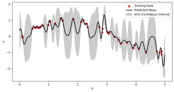
In this code, first generate some sample data points with added noise then define an RBF kernel and create a Gaussian Process Regressor with it. The model is trained on the training data and used to make predictions on the test data. Finally, the results are visualized with a plot showing the training data, the predicted mean, and the 95% confidence interval.
Implementation of Gaussian Process in Python
Scikit Learn
Python
import matplotlib.pyplot as plt
import numpy as np
from scipy import linalg
from sklearn.gaussian_process import kernels,GaussianProcessRegressor
## check version
import sys
import sklearn
print(sys.version)
!python --version
print("numpy:", np.__version__)
print("sklearn:",sklearn.__version__)
The necessary libraries for Gaussian Process Regression (GPR) in Python are imported by this code; these are SciPy for linear algebra functions, NumPy for numerical operations, and Matplotlib for data visualization. To make sure it is compatible with the necessary packages, it additionally verifies the version of Python and prints it, along with the versions of NumPy and scikit-learn (sklearn).
Kernel Selection
Python
np.random.seed(0)
n=50

kernel_ =[kernels.RBF (),

         kernels.RationalQuadratic(),

         kernels.ExpSineSquared(periodicity=10.0),

         kernels.DotProduct(sigma_0=1.0)**2,

         kernels.Matern()
         ]
print(kernel_, '\n')
Output:
[RBF(length_scale=1),
RationalQuadratic(alpha=1, length_scale=1),
ExpSineSquared(length_scale=1, periodicity=10),
DotProduct(sigma_0=1) ** 2,
Matern(length_scale=1, nu=1.5)]
The code specifies the number of test sites (n) and initializes a random seed. In order to display the chosen kernels, it generates a list of several kernel functions and prints the list.
Kernel Comparison and Visualization
Python
for kernel in kernel_:

    # Gaussian process

    gp = GaussianProcessRegressor(kernel=kernel)

    # Prior

    x_test = np.linspace(-5, 5, n).reshape(-1, 1)
    mu_prior, sd_prior = gp.predict(x_test, return_std=True)
    samples_prior = gp.sample_y(x_test, 3)

    # plot

    plt.figure(figsize=(10, 3))
    plt.subplot(1, 2, 1)
    plt.plot(x_test, mu_prior)
    plt.fill_between(x_test.ravel(), mu_prior - sd_prior,
                     mu_prior + sd_prior, color='aliceblue')
    plt.plot(x_test, samples_prior, '--')
    plt.title('Prior')

    # Fit

    x_train = np.array([-4, -3, -2, -1, 1]).reshape(-1, 1)
    y_train = np.sin(x_train)
    gp.fit(x_train, y_train)

# posterior

    mu_post, sd_post = gp.predict(x_test, return_std=True)
    mu_post = mu_post.reshape(-1)
    samples_post = np.squeeze(gp.sample_y(x_test, 3))

    # plot

    plt.subplot(1, 2, 2)
    plt.plot(x_test, mu_post)
    plt.fill_between(x_test.ravel(), mu_post - sd_post,
                     mu_post + sd_post, color='aliceblue')
    plt.plot(x_test, samples_post, '--')
    plt.scatter(x_train, y_train, c='blue', s=50)
    plt.title('Posterior')

    plt.show()

    print("gp.kernel_", gp.kernel_)
    print("gp.log_marginal_likelihood:",
          gp.log_marginal_likelihood(gp.kernel_.theta))

    print('-'*50, '\n\n')
Output:
RBF
gp.kernel_ RBF(length_scale=1.93)
gp.log_marginal_likelihood: -3.444937833462133
---------------------------------------------------
Rational Quadratic
gp.kernel_ RationalQuadratic(alpha=1e+05, length_scale=1.93)
gp.log_marginal_likelihood: -3.4449718909150966
--------------------------------------------------
ExpSineSquared
gp.kernel_ ExpSineSquared(length_scale=0.000524, periodicity=2.31e+04)
gp.log_marginal_likelihood: -3.4449381454930217
--------------------------------------------------
Dot Product
gp.kernel_ DotProduct(sigma_0=0.998) ** 2
gp.log_marginal_likelihood: -150204291.56018084
--------------------------------------------------
Matern
gp.kernel_ Matern(length_scale=1.99, nu=1.5)
gp.log_marginal_likelihood: -5.131637070524745
--------------------------------------------------
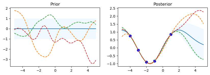
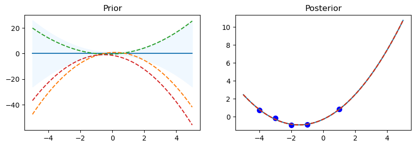
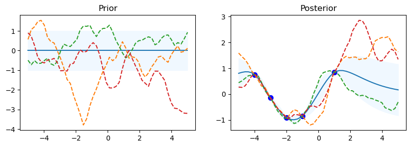
The code starts by looping over the various kernel functions listed in the kernel_ list. A Gaussian Process Regressor (gp) is made using the particular kernel for every kernel. For the Gaussian Process, this establishes the covariance structure. In order to assess the previous distribution, a set of test input points called x_test is established, with values ranging from -5 to 5. This set of points is transformed into a column vector.
Using the gp.predict method, the prior distribution’s mean (mu_prior) and standard deviation (sd_prior) are determined at each test point. Standard deviation values are requested using the return_std=True option. gp.sample_y(x_test, 3) is used to get three function samples from the previous distribution.
The first subplot shows the previous distribution’s mean, with the standard deviation represented by a shaded area. The samples are superimposed as dashed lines, while the mean is displayed as a solid line. There is a subplot called “Prior.” There is a defined set of training data points (x_train) and goal values (y_train) that go with them. The Gaussian Process model is fitted using these points (gp.fit(x_train, y_train)). Five data points with corresponding sine values make up the training data in this code.
Following the training data fitting phase, the procedure computes the posterior distribution’s mean (mu_post) and standard deviation (sd_post) for the same test points (x_test). gp.sample_y(x_test, 3) is also used to produce function samples from the posterior distribution. The second subplot overlays the sampled functions as dotted lines and shows the mean of the posterior distribution, shaded with the standard deviation. Plotted in blue are the training data points. The subplot has the name “Posterior.”
To see the previous and posterior plots for the current kernel and gain a visual understanding of the behavior of the model, call Matplotlib’s plt.show() function.
The code shows details about the current kernel, such as gp.kernel_, which indicates the current kernel being used, and gp.log_marginal_likelihood(gp.kernel_.theta), which gives the log marginal likelihood of the model using the current kernel, after each set of prior and posterior plots.
Advantages of Gaussian Process Regression (GPR)
Gaussian Process Regression (GPR) has a number of benefits in a range of applications:
- GPR provides a probabilistic framework for regression, which means it not only gives point estimates but also provides uncertainty estimates for predictions.
- It is highly flexible and can capture complex relationships in the data.
- GPR can be adapted to various applications, including time series forecasting, optimization, and Bayesian optimization.
Challenges of Gaussian Process Regression (GPR)
- GPR can be computationally expensive when dealing with large datasets, as the inversion of a covariance matrix is required.
- The choice of the kernel function and its hyperparameters can significantly impact the model’s performance.
Good Examples of GPR Applications
- Stock Price Prediction: GPR can be used to model and predict stock prices, taking into account the volatility and uncertainty in financial markets.
- Computer Experiments: GPR is useful in optimizing complex simulations by modeling the input-output relationships and identifying the most influential parameters.
- Anomaly Detection: GPR can be applied to anomaly detection, where it identifies unusual patterns in time series data by capturing normal data distributions.
Conclusion
In conclusion, Gaussian Process Regression is a valuable tool for data analysis and prediction in situations where understanding the uncertainty in predictions is essential. By leveraging probabilistic modeling and kernel functions, GPR can provide accurate and interpretable results. However, it’s crucial to consider the computational cost and the need for expert input when implementing GPR in practice.
Please Login to comment...