

Abstract
Multimodal data analysis has attracted ever-increasing attention in computational biology and bioinformatics community recently. However, existing multimodal learning approaches need all data modalities available at both training and prediction stages, thus they cannot be applied to many real-world biomedical applications, which often have a missing modality problem as the collection of all modalities is prohibitively costly. Meanwhile, two diagnosis-related pieces of information are of main interest during the examination of a subject regarding a chronic disease (with longitudinal progression): their current status (diagnosis) and how it will change before next visit (longitudinal outcome). Correct responses to these queries can identify susceptible individuals and provide the means of early interventions for them. In this article, we develop a novel adversarial mutual learning framework for longitudinal disease progression prediction, allowing us to leverage multiple data modalities available for training to train a performant model that uses a single modality for prediction. Specifically, in our framework, a single-modal model (which utilizes the main modality) learns from a pretrained multimodal model (which accepts both main and auxiliary modalities as input) in a mutual learning manner to (1) infer outcome-related representations of the auxiliary modalities based on its own representations for the main modality during adversarial training and (2) successfully combine them to predict the longitudinal outcome. We apply our method to analyze the retinal imaging genetics for the early diagnosis of age-related macular degeneration (AMD) disease, that is, simultaneous assessment of the severity of AMD at the time of the current visit and the prognosis of the condition at the subsequent visit. Our experiments using the Age-Related Eye Disease Study dataset show that our method is more effective than baselines at classifying patients' current and forecasting their future AMD severity.
Keywords: age-related macular degeneration, genotype, imaging genetics, longitudinal prediction, mutual learning, phenotype
1. INTRODUCTION
Studying integrative imaging genetics has recently been enabled, thanks to the developments in multimodal biomedical imaging and high-throughput genotyping and sequencing tools. Moreover, these innovations present intriguing new possibilities that can serve us to understand various disease pathways. Even though multiple multimodal learning (MML) techniques have been proposed and demonstrated superior performance in integrative analysis of imaging genetics data, two challenges are yet desired to get addressed for practical applications:
1.1. Input data with missing modalities
An ideal scenario is that the researchers or clinicians be able to explore all related data modalities for decision making, that is, diagnosing based on multimodal data. In practice, yet, just one main modality that provides the majority of “signal” concerning a subject's status is often evaluated because of the high expense of gathering other data modalities. For example, it has been studied that genetic factors are crucial to the progression of age-related macular degeneration (AMD) pathogenesis (Fritsche et al, 2016; Fritsche et al, 2013; Wei et al, 2020; Yan et al, 2018). Also, developments in sequencing techniques (Aakur et al, 2021; Metzker 2010; Mikheyev et al, 2014) have made whole-genome sequencing achievable that can provide helpful knowledge for AMD diagnosis. However, in practical settings, subjects' AMD severity score (Ferris III et al, 2013) is typically only assessed by examining their color fundus photographs (CFP), which is the most widely available retinal image modality, because expensive equipment for sequencing is not available, particularly in low-resourced regions.
1.2. Diagnosis and prediction of longitudinal outcome
Many diseases have several severity stages, and a subject may develop to advanced ones as time goes on. Thus, understanding the characteristics of the disease and predicting its progression can help physicians make treatment recommendations. When examining a subject's condition in a clinical setting, two key questions are: Given their examination records, “how the current severity status of them is” (diagnosis), and “how their disease severity will change until their subsequent visit” (longitudinal outcome prediction). Precise responses to these queries can enable physicians to initiate early therapy for vulnerable subjects to slow the course of their disease by thoroughly forecasting a subject's current state and future disease trajectory.
We seek to tackle both challenging tasks in the second aspect while taking the limitations described in the first one into account. First, our intuition is that single-modal input-based models that benefit from the main and auxiliary data modalities gathered in multimodal datasets during training and rely on the main modality in their inference phase, more closely resemble clinical practice. Thus, we use our framework to train such a model. Second, if the duration between the current and subsequent visits is not excessive relative to the average rate of the disease development, we may overcome the longitudinal prediction problem by using the data gathered at the current visit to predict statuses of the current and subsequent visits.
MML (Gao et al, 2020; Garcia et al, 2020; Lin et al, 2021; Wang et al, 2020a; Zellers et al, 2019) and deep mutual learning (DML) (Guo et al, 2020; Zhang et al, 2018) techniques have lately shown notable results. On the one hand, MML techniques can successfully make use of the supervision from various modalities to enhance the classification performance in tasks like video categorization and visual question answering. However, because they need all input modalities to be accessible for inference, they are not always practicable for biomedical problems that frequently have missing modalities. On the other hand, DML techniques have shown that two models that are jointly trained and get feedback from their peers show better generalization than their baseline models, which are trained individually. Therefore, we aim to develop a single-modal model while utilizing the advantages of mutual learning to solve the missing modalities problem of MML approaches for our purpose. To do so, we jointly train our single-modal model with a multimodal one in a mutual manner.
In this article, we present a novel framework based on DML (Guo et al, 2020; Zhang et al, 2018) in which a single-modal model—our model that only requires the main diagnostic modality (e.g., CFP) of a target disease (e.g., AMD) to conduct the predictions—and a pretrained multimodal model that takes the main and auxiliary (genetics and age) data modalities as input evolve together during training. Both models learn to solve our formulated classification problem to simultaneously (1) grade the current disease status of a subject (Advanced or not) and (2) predict their future condition in their next visit (advanced or not, with a predefined time-gap between visits, e.g., 3 years). Furthermore, we hypothesize that genetic and demographic (age) information can provide ‘complementary knowledge’ for a model for longitudinal outcome prediction, particularly in subjects with similar fundus images that their future trajectories may differ because of their genetic differences. Therefore, we design our framework such that the single-modal model learns to infer outcome-related representations of auxiliary modalities using its representations for the main modality from its multimodal colleague using a Riemannian adversarial training scheme.
Then, it aggregates them to make the predictions. Additionally, we employ entropy regularization in the pretraining phase of the multimodal model to prevent it from ignoring noisy auxiliary modalities and concentrating exclusively on the main one. We provide a summary of our contributions as follows:
We introduce a new framework to simultaneously diagnose current status and predict the longitudinal outcome of subjects for disease progression by developing a model that only requires the main diagnostic modality—gathered at the current visit—for its predictions while properly leveraging auxiliary modalities available in the training set to improve final model's performance.
We propose to model the complex interaction between representations of the main and auxiliary modalities by Riemannian Generative Adversarial Networks (GAN).
We design a functional entropy regularized pretraining scheme for the multimodal model to prevent it from shortcut learning to discard the auxiliary modality and only use the more informative main modality.
2. RELATED WORK
2.1. Multimodal learning
MML incorporates information from several modalities to improve predictions for a given task. It has made substantial progress in fields like video comprehension and visual question answering, which leverage a variety of audiovisual and textual inputs (Agrawal et al, 2018; Dancette et al, 2021; Gao et al, 2020; Garcia et al, 2020; Gat et al, 2020; Goyal et al, 2017; Hou et al, 2018; Kim et al, 2018; Lin et al, 2021; Panda et al, 2021; Seo et al, 2021; Uppal et al, 2021; Wang et al, 2020b; Zellers et al, 2019). These studies, however, assume that all modalities are available throughout training and inference, which restricts their direct application to medical problems, where the absence of modalities is a frequent challenge. Reconstructing and restoring missing modalities using the ones that are present is a common solution (Cai et al, 2018; Ma et al, 2021; Shi et al, 2019; Suo et al, 2019; Tran et al, 2017; Tsai et al, 2019; Xu et al, 2017). However, in health care problems with limited training data, reconstruction of extremely high-dimensional modalities like genetics ( dimensional in our problem) is not viable.
Furthermore, predicting some modalities from others may not always be feasible. For example, it makes sense to predict one of RGB and thermal images (Xu et al, 2017) from the other, but it makes no sense to reconstruct the entire genome sequence from fundus images of eyes. Another group of methods proposes variational approaches to deal with missing modalities and model the joint posterior of representations of modalities as a product of experts (Wu et al, 2018). Lee and Van der Schaar (2021) use this method to integrate multiomics data and train modality-specific predictors to ensure representations of individual modalities are learned faithfully. Nonetheless, it is not appropriate to use a modality-specific predictor in the longitudinal prediction of disease outcome for modalities like genetics that are static, whereas a subject's disease severity may change over time. This is true for the approach of Wang et al (2020a) as well that trains modality-specific classifiers with incomplete data pairs and train a final multimodal model using limited complete pairs while distilling (Gou et al, 2021; Hinton et al, 2015; Liu et al, 2021) the knowledge of pretrained models in it.
2.2. Deep mutual learning
In a nutshell, DML concurrently trains two or more models, with each model receiving supervision from the training labels and predictions/representations of the others. Zhang et al (2018) introduced DML and showed that it performs better than knowledge distillation (Gou et al, 2021; Hinton et al, 2015; Liu et al, 2021) methods for image classification. Since then, many DML models have been developed for use in a variety of applications, including image classification (Guo et al, 2020; Lan et al, 2018; Son et al, 2021; Wu et al, 2021), semisupervised learning (Wu et al, 2019), self-supervised learning (Bhat et al, 2021; Wang et al, 2021), and object detection (Qi et al, 2021). These models are not suitable for our problem because they train two models with the same input modality. Recently, Zhang et al (2021) proposed a multimodal image segmentation model to train two single-modal models in a DML manner. However, their multimodal DML idea is intended for problems where their modalities are two “views” of the same phenomenon, not “complementary” modalities like CFP and genetics for AMD where CFP contains the majority of the diagnostic signal while noisy genetics input only complements the knowledge from CFP.
2.3. Age-related macular degeneration
In this article, we analyze the retinal imaging genetics data, which were collected to study the AMD disease and are a good testing platform to evaluate our new method. AMD is a chronic disease (Luu et al, 2018) that causes the progressive decline of vision due to the dysfunction of the central retina in older adults and is the major root of blindness in elder Caucasians (Bird et al, 1995; Congdon et al, 2004; Trucco et al, 2019). Based on a scale called AMD severity score, three stages are defined for AMD: early, intermediate, and late (advanced) (Ferris III et al, 2013). The severity score is determined by exploring characteristics of the CFP of subjects. The main symptom of the early and intermediate stages is the presence of yellowish deposits called “drusen” in the retina, and most patients are asymptomatic in them (Ayoub et al, 2009; Grassmann et al, 2018). The irreversible stage that is accompanied by severe vision loss is late AMD that appears in two forms: “Dry” and “Wet.” In dry AMD (Geographic Atrophy), accumulation of drusen in the retina decreases its sensitivity to light stimuli and causes gradual loss of central vision.
In wet AMD (Choroidal Neovascularization), the growth of leaky blood vessels under the retina damages photoreceptor cells and affects visual acuity. Some CFPs with their AMD symptoms and labels from the Age-Related Eye Disease Study (AREDS) (The Age-Related Eye Disease Study Research Group, 1999) dataset are shown in Section 2.3.1. GWAS studies have shown that genetic and environmental factors are critical elements associated with AMD (Fritsche et al, 2016; Fritsche et al, 2013; Wei et al, 2020) and its progression time (Yan et al, 2018). In recent years, multiple deep learning-based predictive models are proposed for AMD.
They have two categories: (1) diagnostic models that predict AMD severity of a subject based on their CFP taken at their current visit (Burlina et al, 2018; Burlina et al, 2017; Burlina et al, 2016; Grassmann et al, 2018; Keenan et al, 2019; Peng et al, 2019). Although these models have shown convincing performance for the diagnosis task, they cannot predict subjects' longitudinal outcome that is crucial information for clinicians to start preventive treatments for vulnerable subjects. (2) Models predicting whether a subject progresses into late AMD in less than “n” years (Bridge et al, 2020; Peng et al 2020; Yan et al, 2020), where “n” is a predefined value. Nonetheless, if their answer is yes, they do not provide any information about whether the subject is already in advanced AMD or they will progress to it in the future. Furthermore, the majority of previous works are single-modal based on CFPs that waste genetic modality in training datasets or they are multimodal (Peng et al, 2020; Yan et al, 2020) taking CFPs and 52 AMD-associated variants (Yan et al, 2018), which limits their practicality because they need genetic modality in their inference phase.
2.3.1. AMD characteristics in CFPs
Based on a 12-scale score called AMD severity, three stages are defined for AMD: Early, Intermediate, and Advanced (Ferris III et al, 2013). The main characteristics of AMD are (1) the presence of drusen in the macula and (2) growth of leaky blood vessels under the retina. We demonstrate these cases with samples from AREDS dataset (The Age-Related Eye Disease Study Research Group, 1999) in the following.
2.3.1.1. Normal/early AMD CFPs
Figure 1 shows samples that are normal or in the early stages of AMD. In each image, the macular region is approximately shown by the black circle, and the fovea is the dark center of these circles. These cases have no drusen or leaky blood vessels under their macula.
FIG. 1.

Samples with early-stage AMD or normal. Macular regions are shown by black circles. AMD, age-related macular degeneration.
2.3.1.2. Intermediate AMD
The main symptom of intermediate stages is the presence of drusen in the retina, and most patients are asymptomatic (showing no symptoms) in these stages (Ayoub et al, 2009; Grassmann et al, 2018). Figure 2 illustrates these stages.
FIG. 2.

Samples in intermediate stages of AMD. Black arrows show relatively small area of accumulation of yellow deposits called drusen in the retina.
2.3.1.3. Advanced AMD
The irreversible stage that is accompanied with severe vision loss is late AMD that usually appears in two forms: Dry and Wet.
2.3.1.4. Dry AMD (geographic atrophy)
In dry AMD, accumulation of drusen in retina decreases its sensitivity to light stimuli and causes gradual loss of central vision. It is shown in Figure 3.
FIG. 3.

Samples of the geographic atrophy condition. Black arrows show large areas of accumulation of drusen in the retina.
2.3.1.5. Wet AMD (choroidal neovascularization)
In wet AMD, the growth of leaky blood vessels under the retina damages photoreceptor cells and affects visual acuity. It is shown in Figure 4.
FIG. 4.

Samples of the Choroidal Neovascularization condition. Black arrows show leaked blood from leaky blood vessels in the retina.
3. METHODOLOGY
We develop an adversarial mutual learning framework capable of utilizing auxiliary modalities (genetics and age) available in training set to improve the training of a single-modal model (using only main modality (CFP) that simultaneously addresses main queries regarding a subject's status when a chronic disease is concerned that are: (1) the current status of a subject (e.g., current AMD severity) and (2) how their status will change until their next visit (e.g., how their AMD severity score will change in the near future, i.e., longitudinal outcome) if they maintain their current lifestyle and disease progression trajectory. This knowledge empowers practitioners to start early treatment to decelerate the disease progression for susceptible subjects. We explain the intuitions behind our model step by step in the following subsections using AMD terminologies, but as we noted, it is applicable for similar diseases as well. Our procedure can be seen in Figure 5.
FIG. 5.

Overview of our framework. Left: pretraining of our multimodal M-model. CFP and genetic information of subjects are used to train the model. CFP contains the majority of the “diagnostic signal” related to AMD. Thus, to prevent the model to get biased toward CFP and discard the genetic modality, we impose entropy regularization using a Gaussian measure on the model during training (Section 3.3.1). Right: mutual learning of our single-modal S-model (top) with the pretrained M-model (bottom). S-model learns from the M-model to infer joint AMD-related representations of the genetic and demographic modalities—using its representations for an input CFP—using a Riemannian GAN model. The backbone of the S-model gets initialized by the weights of the CFP-Net of the M-model, and the M-model evolves during training by updating its CFP-Net using the EMA of the weights of the S-model's backbone (Section 3.3.2). CFP, color fundus photograph; EMA, exponential moving average; GAN, generative adversarial networks.
3.1. Problem formulation
We formulate our prediction task as a classification problem. Considering AMD severity condition of a subject in their current and next visits (with a predefined time gap between them e.g., years), we define three classes: (1) if a subject is not in the advanced AMD condition and will not progress to it until their next visit. (2) if they are not currently in the advanced stage but will progress to advanced AMD until their next visit. (3) if they have already progressed to the advanced phase. As there is no treatment for late AMD yet (Trucco et al, 2019), the fourth case for (current, next) (advanced, not advanced) is not possible. Our goal is to develop a model that accurately classifies subjects into one of the mentioned classes based on their current visit's CFP images. This formulation enables us to overcome the challenge of heterogeneity of time gaps between consecutive visits for subjects in longitudinal datasets. For instance, we can use records of a subject at visit numbers to train a model with with pairs , but a sequence model should handle uneven time gaps between successive visits.
3.2. Notations
Let us assume that we have a longitudinal dataset such as AREDS (The Age-Related Eye Disease Study Research Group, 1999) in which each subject has a random number of records corresponding to the visit time points that their data are collected during the study. We denote the training dataset as where N is the number of subjects, T is the set of all possible visit indices during the study, Ti is the set of available visit indices for the i-th subject, is the fundus image of the subject taken during the visit with index tj, and is the genetic modality of the subject, which is static. For example, in the AREDS dataset (The Age-Related Eye Disease Study Research Group, 1999), examinations are performed every 6 months, and the maximum follow-up study length for a subject is 13 years (26 visits). Thus, is the set of all possible visit numbers. In addition, we denote our single-modal model as S-model and multimodal as M-model in the rest of the article.
3.3. Longitudinal predictive model
We introduce an adversarial mutual learning framework in which the single-modal S-model learns from a pretrained multimodal M-model to (1) infer outcome-related joint representation of genetics and demographics (age) from its representations for input CFPs using a Riemannian GAN model—inspired by studies (Fritsche et al, 2016; Fritsche et al, 2013; Wei et al, 2020; Yan et al, 2018) that have established high association between these modalities and AMD severity outcome that makes it reasonable to incorporate such prior in our model—and (2) combining the predicted representation and the one for the visual modality to solve longitudinal outcome classification task in the course of a mutual training scheme (Guo et al, 2020; Zhang et al, 2018) that benefits both models. In summary, our algorithm consists of pretraining the multimodal M-model and mutual training the S-model along with the M-model. We describe details of each one in the following.
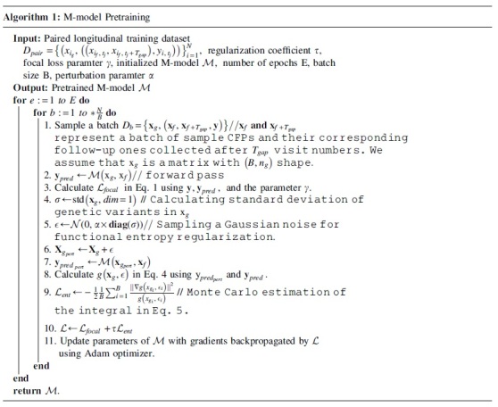
3.3.1. M-model pretraining
We use a multimodal M-model to guide the training process of the S-model in a mutual learning fashion. The architecture of the M-model is shown in Figure 5. It consists of two subnetworks: (1) CFP-net: ResNet (He et al, 2016) backbone for CFP modality and (2) GD-net: a feed-forward model that combines genetic as well as demographic (age) modalities to obtain a joint outcome-related representation for them. Finally, obtained representations are combined in an early fusion (Baltrušaitis et al (2018) scheme and passed to a classifier to perform prediction.
As the number of samples in the case group (advanced AMD condition) is far less than the control group in our problem, our classification problem is imbalanced. We use Focal loss (Lin et al, 2017) to train the M-model because it down-weights the contribution of “simple” examples from majority classes (e.g., control cases without any symptoms that the model can easily classify) in the loss function that the model is already confident about them. Formally, given yi is the correct class corresponding to a sample x and be the predicted conditional probability of our teacher model for class yi given x, Focal loss for the training sample is calculated as

where is a hyperparameter controlling the down-weighting factor. As can be seen, Focal loss is a scaled version of Cross-Entropy loss that has a lower value for confident predictions of the model.
As we mentioned, the CFP of subjects contains the majority of the “diagnostic signal” regarding their AMD status, and the genetics modality provides complementary knowledge with a much lower signal-to-noise ratio compared with the CFP modality. Therefore, directly training the model with Focal loss and standard regularization schemes for deep learning training, such as -norm of weights that prefers networks with simpler structures may bias the model to discard the genetic modality and only focus on the CFP one. This phenomenon has been observed in the literature for domains such as visual question answering (Agrawal et al, 2018; Dancette et al, 2021; Goyal et al, 2017). To overcome this problem, we use functional entropy regularization that balances the contribution of modalities. The intuition is that if our model's predictions show high entropy when we perturb a modality, then it is not bypassing the modality. Formally, given a probability measure over the space of input of a non-negative function , functional entropy of g is defined as (Bakry et al, 2014):
| (2) |
However, the calculation of the RHS of this equation is intractable. As a workaround, Logarithmic Sobolev Inequality (Bakry et al, 2014; Gat et al, 2020) is calculated as an upper bound of the functional entropy for Gaussian measures :
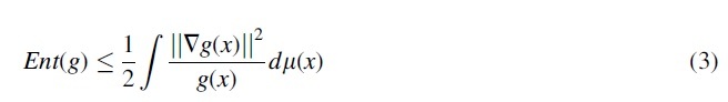
In our problem, we define g as a measure of a discrepancy between the softmax output distribution of the M-model when the original genetics modality and its Gaussian perturbed version of it are inputted to the model while keeping the input CFP fixed. In other words, given an input sample :

The function g defined in Eq. (4) can represent the sensitivity of the model's predictions to Gaussian perturbations of the genetic modality. Now, we plug g into Eq. (3) and define a loss function , which encourages the model to have high functional entropy w.r.t its genetics input:

In practice, we estimate the integral using Monte Carlo sampling, that is, we approximate it with one for each sample. In addition, we set as a diagonal covariance matrix with diagonal elements being the empirical variance of samples in the batch in each iteration. We provide the pseudocode for pretraining the M-model in Algorithm 1.
3.3.2. Mutual learning of S-model and M-model
After pretraining the M-model, we develop a training scheme based on mutual learning to train the S-model. As shown in Figure 5, S-model has a backbone identical to CFP-net in M-model and a “predictor” module. We aim to embed two prior medical knowledge into the inductive bias of our model that are: (1) high association between AMD severity and genetic variants (Fritsche et al, 2016; Fritsche et al, 2013; Wei et al, 2020; Yan et al, 2018). (2) The ability of fundus images to predict the age of subjects (Wen et al 2020). To do so, we use the predictor module inside the S-model to predict representations of GD-net of the M-model. This prediction will be in a much lower dimensional space than reconstructing/imputing the whole genetic and age modalities together (Cai et al, 2018; Ma et al, 2021; Shi et al, 2019; Suo et al, 2019; Tran et al, 2017; Xu et al, 2017), and thus, is more sample efficient. The distribution of joint representation of genetics and age given the representation of CFP images may be multimodal, that is, the mapping between them not necessarily be bijective.
Thus, we train the predictor subnetwork of the S-model using GAN that are capable of modeling complex high-dimensional distributions (Arjovsky et al, 2017; Goodfellow et al, 2014; Gulrajani et al, 2017).
3.3.2.1. Modeling interactions between representation of a CFP and corresponding joint representation of genetics and age
We formulate learning such complex interaction with Riemannian GAN (Park et al, 2019; Shim et al, 2020) training. In summary, GAN (Arjovsky et al, 2017; Goodfellow et al, 2014; Gulrajani et al, 2017; Park et al, 2019; Shim et al, 2020) models are trained using a two-player game in which a generator model G aims to learn the underlying distribution of a set of samples in the training set to trick a discriminator model D that distinguishes whether its input is real or a fake one generated by G. As the training process advances, the generator learns the distribution of training samples, and the discriminator will not be able to differentiate between real and fake samples generated by G. Conventional GAN models' discriminators (Goodfellow et al, 2014) measure the distance between real and fake samples using Euclidean distance between their low dimensional embeddings. However, it is shown that (Arvanitidis et al, 2021; Edraki et al, 2019; Shim et al, 2020) models are trained using a two-player game in which a generator model G aims to learn the underlying distribution of a set of samples in the training set to trick a discriminator model D that distinguishes whether its input is real or a fake one generated by G. As the training process advances, the generator learns the distribution of training samples, and the discriminator will not be able to differentiate between real and fake samples generated by G. Conventional GAN models' discriminators (Goodfellow et al, 2014) measure the distance between real and fake samples using Euclidean distance between their low dimensional embeddings. However, it is shown that (Arvanitidis et al, 2021; Edraki et al, 2018) such distance may not faithfully reflect distances of data points as it is well known that high-dimensional real-world data are not randomly distributed in the ambient space and are often restricted to a nonlinear low-dimensional manifold (Tenenbaum et al, 2000) with unknown intrinsic dimension.
Therefore, Riemannian GAN models' discriminators, project low-dimensional representations of samples on a Riemannian manifold such as hypersphere (Park et al, 2019; Shim et al, 2020) and calculate distances between them with the length of geodesics connecting them on the manifold. Distances on hypersphere are limited, which makes the training stable, and it is shown that (Park et al, 2019) training GAN with geodesic distances on hypersphere is equivalent to minimizing high-order Wasserstein distances between real and fake distributions and generalizes methods that minimize the 1-Wasserstein distance (Arjovsky et al, 2017; Gulrajani et al, 2017).
Formally, we define a unit hypersphere with a center c and the main axis direction u () that are learnable. Given a joint representation on genetics and age (can be real predicted by GD-net of M-model or fake one by predictor of S-model) input () to the discriminator, it projects h into a d-dimensional space using nonlinear layers to obtain an embedding g. Then, it projects g on the unit sphere with center c such that . Now, let's consider circular cross-sections of the hypersphere that the main axis u of the hypersphere is the normal vector of the surface that they lie in. The idea is that if the discriminator gets designed to distinguish between real and fake samples based on the closeness of the cross-section that they lie on to the greatest circle of the hypersphere—that is, the larger the radius of the cross-section that a sample lies on, more realness score is assigned to it—then, the generator will attempt to generate samples that are on the largest circle of the hypersphere.
Therefore, it will be able to generate more diverse samples, which prevents mode collapse. Given a batch of samples , we calculate for each sample hj and decompose it as . The output score of the discriminator for a sample hj is calculated as:
| (6) |
where and are empirical variances of and , respectively. We use the relativistic objective (Jolicoeur-Martineau, 2019) to train the GAN model. In a nutshell, it is designed such that the generator not only attempts to increase the score of the discriminator for fake samples, but also aims to decrease its score for real samples. If we denote joint representations of GD-net in M-model by and the ones predicted by the predictor model of S-model with objectives of G (predictor in S-model) and discriminator D are as follows:
| (7) |
| (8) |
where calculates the discriminator's estimated probability that one/batch of real sample[s] is/are more realistic than a batch/one fake one[s], and is a hyperparameter Jolicoeur-Martineau (2019). We train the parameters for the main axis u and center c as follows. In each iteration, given a batch of real and fake samples , at first, we update the center parameter with:

is the Huber function (Huber, 1992), and the objective estimates the center of the hypersphere given a batch of samples. Then, we fix the center parameter, and to make the training of the center parameter stable, we encourage the discriminator to map samples to embeddings with similar distances relative to the center, that is,

where is the empirical standard deviation (SD) of distances from projected embeddings to the center. Parameters of the main axis u and discriminator are updated with backpropagated gradients from loss functions in Eqs. (7 and 10).
We train the S-model's classifier to combine its representation for CFP and the predicted joint one for genetic and demographic modalities to accurately classify subjects' status. First, we use Focal loss (Lin et al 2017) defined in Eq. (1) to leverage training labels. Second, we use a distillation loss (Hinton et al, 2015) to guide the S-model using predictions of the M-model:
| (11) |
where the parameter T is a temperature parameter that controls the sharpness of output softmax distributions of models. In summary, the training objective for S-model's training is:
| (12) |
Before starting training of the S-model, we initialize its backbone with the weights of the pretrained M-model's CFP-net to make the convergence faster. As adversarial training may cause instability and degradation of the backbone's representations (Chavdarova et al, 2018; Goodfellow, 2016; Tao et al, 2020), we do not backpropagate gradients from adversarial training for the backbone's weights. Instead, we train them using supervision from Focal loss and distillation loss. Finally, as shown that mutual learning benefits from both models getting feedback from their peers, we update M-model's CFP-net's weights with exponential moving average (EMA) of the backbone of the S-model, that is, after each iteration, we update CFP-net's weights as:
| (13) |
Doing so prevents corruption of the weights of pretrained M-model happening when using well-known distillation loss from S-model to M-model (Guo et al, 2020; Zhang et al, 2018) in the starting phase of training as S-model's predictions are not reliable yet. We summarize our mutual training algorithm in Algorithm 2.
4. EXPERIMENTS
In this section, we evaluate the effectiveness of our proposed adversarial mutual learning method on the task of simultaneously grading the current AMD severity of a subject as well as predicting their longitudinal outcome in their next visit when the predefined time gap between visits are 2, 3, and 4 years, respectively. We compare our model with baseline methods, provide its interpretations, and perform an ablation study to analyze the effect of its different components.

4.1. Experimental setup
4.1.1. Data description
We use AREDS dataset (The Age-Related Eye Disease Study Research Group, 1999) for our experiments, which is the largest longitudinal dataset available for AMD collected and maintained by the National Eye Institute (NEI). It is available at the dbGaP*. AREDS contains longitudinal CFPs of 4628 participants, and a subject may have up to 13-year follow-up visits since the baseline. For preprocessing step, we cropped each CFP to a square that encompasses the Macula (Burlina et al, 2017; Peng et al, 2019) and resized it to pixel resolution. As mentioned in Section 1, the yellowish color of drusen in the macula and the red color of leaky blood vessels are important characteristics of dry and wet AMD, respectively. Thus, we use a nonlinear Bézier augmentation (Zhou et al, 2019)—previously proposed for Computed tomography (CT) scans and X-ray data—followed by random vertical and horizontal flip to augment CFPs. In addition to CFPs, genome sequence of 2780 () subjects is available in AREDS.
We use all the genetic variants that are in the 34 loci regions (Fritsche et al, 2016) associated with advanced AMD with minor allele frequency 0.01 (Fritsche et al, 2016), and 156,864 SNPs remain after filtering. We then partition the AREDS dataset on the subject level and take all subjects that their genetic information is available as our train set. We randomly partition the rest into two halves for our validation and test sets.
4.1.1.1. Data pairing
We define our classification task as simultaneously (1) grading current AMD status of a subject (advanced or not) and (2) predicting their condition in their next visit (advanced or not, with a predefined time gap between visits ) given their CFP at the current visit. We denote our training dataset with such that is the genetic modality of the i-th subject that is static, is a CFP of the i-th subject taken at their visit number tj, and is the 12-scale severity score (1–12) of the CFP . Subjects in AREDS (The Age-Related Eye Disease Study Research Group, 1999) may have up to 13 years follow-up records that are collected every 6 months. Therefore, the set of all possible visit numbers are , and . We denote all visit numbers available for the i-th subject with Ti, and due to missing visits, Ti may be any subset of T. To train our model, we make pairs of samples from visit numbers available for subjects in Algorithm 3.

4.1.1.2. CFP images
We used left-side Field 2 (30° imaging field centered at the fovea) stereoscopic CFPs (Age-Related Eye Disease Study Research Group, 2001) of subjects as this angle focuses on macula, which is the most significant region related to AMD. We determine whether an eye has progressed to advanced AMD using the 12-scale severity score (1–12) available in the AREDS (The Age-Related Eye Disease Study Research Group, 1999) dataset, namely we consider severity score 9–12 as being in the advanced condition and not advanced otherwise. We defined our classification task as simultaneously grading current AMD severity of a subject and their condition in their next visit, that is, their longitudinal outcome when the time gap between visits be 2, 3, and 4 years. For each of these cases, we provide the number of pairs for our train, validation, and test sets in Table 1.
Table 1.
Number of Data Pairs Used in Different Settings
| Time gap | Partition | Number of pairs |
|||
|---|---|---|---|---|---|
| Y = 0 (Not Adv, Not Adv) | Y = 1 (Not Adv, Not Adv) | Y = 2 (Not Adv, Not Adv) | Sum | ||
| 2 years | Train | 5548 | 1176 | 4577 | 11,301 |
| Validation | 1465 | 266 | 942 | 2673 | |
| Test | 1417 | 241 | 913 | 2673 | |
| 3 years | Train | 5218 | 1430 | 3742 | 10,390 |
| Validation | 1315 | 308 | 715 | 2338 | |
| Test | 1262 | 261 | 700 | 2223 | |
| 4 years | Train | 5065 | 3117 | 1601 | 9783 |
| Validation | 1163 | 312 | 544 | 2019 | |
| Test | 1076 | 267 | 509 | 1852 | |
Not Adv, not advanced.
4.1.1.3. Nonlinear Bézier augmentation for CFPs
As the yellow color of drusen and red one for leaky blood vessels in the retina are important to evaluate AMD characteristics, we use the nonlinear Bézier transform that preserves order of pixels' intensity and their color to augment our training CFPs. It can properly mimic different lighting conditions that fundus images may have been taken in them by weakening or reinforcing pixels' intensities and was introduced by Zhou et al (2019) for augmenting CT and X-ray images for self-supervised learning. In summary, the transformation applies a nonlinear monotonic function on pixels' intensities. The function is based on Bézier Curve (Mortenson, 1999) that is characterized by four points: as two endpoints, and that are control ones. In practical implementation, a step size parameter t is used that determines the precision of mapping. Given four points and step size t, curve points such that ( are calculated as:

Then, for a new intensity value , the output intensity value y is estimated by linear interpolation of the point with the points and . An example of a monotonic Bézier curve is shown in Figure 6. To enforce increasing monotonicity of the function, and are fixed, and to make the transformation stochastic during training, the points P1 and P2 are sampled randomly. Some CFPs and their random Bezier augmentations are shown in Figure 7.
FIG. 6.

A sample Bézier curve with points .
FIG. 7.

Examples of the nonlinear Bézier augmentation combined with random horizontal and vertical flip on Age-Related Eye Disease Study (AREDS) Research Group (2001) samples. Images on the left column are original samples, and the ones on the other columns are transformed versions. AREDS, Age-Related Eye Disease Study.
4.1.2. Baselines
We compare our method against previous mutual learning and knowledge distillation methods in the literature. DML Zhang et al (2018) trains two models from scratch with different initialization such that each model is trained with a loss function that is the sum of two terms, namely Cross-Entropy loss and KL-divergence between the distributions predicted by the model and its peer. Knowledge Distribution via Collaborative Learning (KDCL) (Guo et al, 2020) improves DML by using “ensemble” of models' predictions instead of prediction of the peer model in the KL-divergence term. We use two ensemble schemes for KDCL, namely “min-logit” and “mean.” Knowledge Distillation (KD) (Hinton et al, 2015) distills the knowledge in the powerful large pretrained model, called teacher model, into a model, student, by training the student model using KL-divergence loss between its predictions and the ones for the teacher model. In addition, to show the effectiveness of leveraging “complementary” knowledge in the genetics modality, we compare our model with single-modal baselines such that we train a ResNet architecture with Focal loss and Cross-Entropy loss. We denote these two cases in our experiments as Base-Focal and Base-Cross Entropy (Base-CE).
4.1.3. Training and evaluation
We use multiclass Area Under Curve introduced by Hand and Till (Hand et al, 2001) as our evaluation metric because it is suitable for imbalance classification problems and has been used in AMD literature (Burlina et al, 2017; Peng et al, 2020; Peng et al, 2019; Yan et al, 2020). We pretrain our M-model for 10 epochs with batch size 128. Then, we train S-model mutually with M-model for 10 epochs with batch size 32. We use the same architectures for two subnetworks of all other mutual learning and knowledge distillation methods, and we use the architecture of our S-model for Base-CE/Focal. By doing so, we reduce the effect of architectural design and can more readily compare the methods. For a fair comparison, we train all baseline models for 20 epochs with batch size 128. We use Adam optimizer (Kingma et al, 2015) with learning rate , exponential decay rates , and weight decay for all models, except for the parameters of the S-model's predictor and discriminator that we set , and also, initialize their parameters with normal distribution with zero mean and SD of 0.02.
4.1.4. Architectures
4.1.4.1. M-model
We use ResNet-18 (He et al, 2016) architecture until its global average pooling layer for the CFP-Net of the M-model. For GD-Net, we used a feed-forward model with three hidden layers with dimensions 128—257—256 and ReLU activation followed by BatchNorm layer (Ioffe et al, 2015). The layer with 257 dimensions is a concatenation of 256 output feature representations of the previous layer and a single value for the age of subjects at the visit number of the input CFP image to the CFP-Net. The age values are normalized to the interval using minimum and maximum values in the training set. We use a fully connected layer with three outputs for M-model's classifier.
4.1.4.2. S-model
We use the same architecture of the CFP-Net of the M-model for the backbone of the S-Model. For GAN's generator architecture, we use two Residual blocks with the following architectures. The architectures' blocks are written in the PyTorch Paszke et al (2019) terminology:
Residual Block #1: BatchNorm1d(512) LeakyReLU(negative slope = 0.2) Linear(512, 512) BatchNorm1d(512) LeakyReLU(negative slope = 0.2) Linear(512, 512) Residual Connection Dropout(0.5)
- Residual Block #1 Shortcut: Linear(512, 512)
Residual Block #2: BatchNorm1d(512) LeakyReLU(negative slope = 0.2) Linear(512, 256) BatchNorm1d(512) LeakyReLU(negative slope = 0.2) Linear(256, 256) Residual Connection Dropout(0.5)
- Residual Block #2 Shortcut: Linear(512, 256)
4.1.4.3. Discriminator
Our discriminator calculates the representation g for an input sample h using a feed-forward block followed by a dropout and two Residual blocks.
Feed-forward Block: LeakyReLU(negative slope = 0.2) Linear(256, 256) LeakyReLU(negative slope = 0.2) Dropout(0.5).
Residual Block #1: BatchNorm1d(256) LeakyReLU(negative slope = 0.2) Linear(256, 256) BatchNorm1d(256) LeakyReLU(negative slope = 0.2) Linear(256, 256) Residual Connection Dropout(0.5)
- Residual Block #1 Shortcut: Linear(256, 256)
Residual Block #2: BatchNorm1d(256) LeakyReLU(negative slope = 0.2) Linear(256, 128) BatchNorm1d(128) LeakyReLU(negative slope = 0.2) Linear(128, 128) Residual Connection Dropout(0.5)
- Residual Block #2 Shortcut: Linear(256, 128)
4.1.5. Hyperparameters
We tuned for focal loss from the set and found that works best for all methods. For KDCL (Guo et al, 2020), we tuned the temperature parameter T from and found that has better performance. We tuned the coefficient of its distillation loss from and observed that is the optimal choice. For KD (Hinton et al, 2015), we searched for its temperature parameter in and found that performs better. For our model, we empirically set the parameters to 1 and set the EMA parameter —for updating the CFP-Net network of the M-model with the backbone of the S-model—to 0.9995. For all models, we tune the weight decay parameter from and found that 0.0001 works reasonably well.
4.2. Experimental results
4.2.1. Comparison with baselines models
Table 2 summarizes the performance of baseline methods and our adversarial mutual learning scheme for simultaneously grading and longitudinal prediction of AMD status of subjects. We explore baseline methods in two settings: (1) genetics modality is incorporated in their training where a multimodal network is trained along with a single-modal one, and we denote them with (M ↔ S). (2) Only CFP is used in their training, and two single-modal models are trained together that are shown by (S ↔ S). It can be seen that mutual learning models consistently outperform knowledge distillation and standard single-network training baselines Base-CE/Focal, which is consistent with observations for natural image classification tasks (Guo et al, 2020; Zhang et al, 2018). Interestingly, Base-Focal has a competitive or even better performance compared with KD (S ↔ S) and shows better results compared with Base-CE, which shows the superior ability of the Focal loss (Lin et al, 2017) to handle long-tailed distributions compared with Cross-Entropy loss.
Table 2.
Comparison of Our Proposed Method with Baseline Methods
| Time gap |
2 years |
3 years |
4 years |
|
|---|---|---|---|---|
| Method | Using auxiliary modality | AUC | ||
| KDCL - MinLogit (M ↔ S) (Guo et al 2020) | ✓ | 0.882 ± 0.003 | 0.881 ± 0.004 | 0.889 ± 0.003 |
| KDCL - MinLogit (S ↔ S) (Guo et al 2020) | × | 0.883 ± 0.004 | 0.880 ± 0.003 | 0.886 ± 0.004 |
| KDCL - Mean (M ↔ S) (Guo et al 2020) | ✓ | 0.876 ± 0.005 | 0.881 ± 0.003 | 0.889 ± 0.002 |
| KDCL - Mean (S ↔ S) (Guo et al 2020) | × | 0.869 ± 0.004 | 0.874 ± 0.003 | 0.886 ± 0.005 |
| DML (M ↔ S) (Zhang et al 2018) | ✓ | 0.879 ± 0.002 | 0.877 ± 0.004 | 0.898 ± 0.003 |
| DML (S ↔ S) (Zhang et al 2018) | × | 0.872 ± 0.004 | 0.874 ± 0.004 | 0.896 ± 0.004 |
| KD (M ↔ S) (Hinton et al 2015) | ✓ | 0.872 ± 0.002 | 0.877 ± 0.003 | 0.888 ± 0.003 |
| KD (S ↔ S) (Hinton et al 2015) | × | 0.867 ± 0.003 | 0.873 ± 0.001 | 0.884 ± 0.001 |
| Base-CE | × | 0.862 ± 0.005 | 0.867 ± 0.005 | 0.877 ± 0.005 |
| Base-focal | × | 0.866 ± 0.003 | 0.877 ± 0.005 | 0.881 ± 0.008 |
| AdvML (ours) | ✓ | 0.896 ± 0.001 | 0.899 ± 0.001 | 0.914 ± 0.001 |
Mean and SD of five runs with different initialization are reported.
AUC, area under curve; AdvML, adversarial mutual learning; CE, cross entropy; DML, deep mutual learning; KD, knowledge distillation; KDCL, knowledge distillation via collaborative learning; SD, standard deviation.
In all cases, except KDCL-MinLogit with 2 years gap, incorporating the genetics modality in the training procedure of the methods enhances the performance of the final single-modal model in inference, which supports our hypothesis that the genetics modality can provide supervision that is beneficial to the model's training. Furthermore, our model outperforms mutual learning models in all three cases of 2-, 3-, and 4-year gaps between visits that demonstrates our model can more effectively “denoise” the highly noisy genetics modality during training compared with other baselines and properly learn to predict AMD-related joint representation of genetic and demographic modalities from its own one for an input CFP and combine them to perform longitudinal prediction.
4.2.2. Interpretation of S-model's predictions
Figure 2 demonstrates gradient-weighted class activation mapping (Grad-CAM) (Selvaraju et al, 2017) saliency maps of our S-model. As mentioned in Section 1 and Section 2.3, the main characteristics of AMD in CFPs are the accumulation of yellow deposits called drusen in the macula of an eye as well as the growth of leaky blood vessels under the retina that cause leakage of blood on photoreceptor cells. Saliency maps in Figure 8 indicate that our S-model looks for these characteristics in the macula for decision making, which is aligned with the clinical practice.
FIG. 8.

Grad-CAM Selvaraju et al (2017) saliency maps of our S-model's decisions. It focuses on the macular region of the eyes and AMD symptoms, namely leaky blood vessels in the retina and yellow deposits in the macula called drusen, which is aligned with clinical practice. Left: neither drusen nor leaky vessels are present in the macula. Middle: small areas of accumulation of drusen are observable. Right: leaked blood in the retina (top) and large areas of drusen (bottom) in the macula exist. CAM, class activation mapping.
4.2.3. Ablation study
In this section, we perform an ablation study to explore the effect of each component of our model. We remove entropy regularization in M-model's pretraining and the GAN training component in the mutual learning both separately and simultaneously. Table 3 summarizes the results. We can observe that removing entropy regularization for the genetics modality causes more severe performance degradation for our model, which highlights its importance to properly “debias” the multimodal model to not neglect the genetics modality and only rely on the CFPs and effectively denoise it to extract its discriminative features for classification.
Table 3.
Ablation Experiments' Results for Different Components of Our Method
| Time gap |
2 years |
3 years |
4 years |
|---|---|---|---|
| Ablation experiment | AUC | ||
| W/O Ent Reg | 0.880 ± 0.000 | 0.885 ± 0.001 | 0.887 ± 0.002 |
| W/O GAN | 0.881 ± 0.001 | 0.889 ± 0.002 | 0.903 ± 0.002 |
| W/O Ent Reg and GAN | 0.871 ± 0.002 | 0.879 ± 0.003 | 0.882 ± 0.001 |
GAN, generative adversarial networks.
5. CONCLUSION
In this article, we introduced a new adversarial mutual learning framework that is capable of leveraging several auxiliary diagnostic modalities (containing complementary diagnostic signals that are collected in the training set and missing in inference) to train a more accurate single-modal model, which uses the main modality (that provides the majority of diagnostic signal and is available in both training and inference) for inference. To do so, the single-modal model is trained with a pretrained multimodal model in a mutual learning manner. We imposed entropy regularization on the multimodal model during its pretraining to encourage it not to neglect the auxiliary modality in its decisions and learn to “denoise” them to keep their discriminative information. Our single-modal model learns from the multimodal one to infer joint representation of the auxiliary modalities from its representation for the main modality and effectively combine them for its predictions. We modeled the complex interaction between modalities using a Riemannian GAN model and defined our classification task as simultaneous diagnosis of the current status of a subject as well as predicting their longitudinal outcome.
We applied our method to the problem of early detection of AMD in which our experiments on the AREDS dataset and our ablation study demonstrated the superiority of our model compared with baselines and the importance of each component for our model.
ACKNOWLEDGMENT
The authors acknowledge the AREDS group at the NEI for providing the AREDS dataset.
AUTHORs' CONTRIBUTIONS
A.G. contributed to methodology development, implementing the models, conducting the experiments, and writing the article; J.Z. did the initial data cleaning and preparation steps and contributed to writing the article; S.Y. worked on data cleaning and processing; W.C. and H.H. supervised the project and contributed to methodological development as well as revising the article.
AUTHOR DISCLOSURE STATEMENT
The authors declare they have no conflicting financial interests.
FUNDING INFORMATION
W.C. is supported by the National Institute of Health grant EY030488; A.G. and H.H. are partially supported by the National Science Foundation IIS grants 1845666, 1852606, 1838627, 1837956, 1956002, and 2040588, and the National Institute of Health grants U01AG068057 and R01EB034116. This research was supported in part by the University of Pittsburgh Center for Research Computing through the resources provided.
REFERENCES
- Aakur SN, Narayanan S, Indla, et al. Mg-net: Leveraging pseudo-imaging for multi-modal metagenome analysis. In International Conference on Medical Image Computing and Computer-Assisted Intervention. Springer; 2021; pp. 592–602. [Google Scholar]
- Age-Related Eye Disease Study Research Group. The age-related eye disease study system for classifying age-related macular degeneration from stereoscopic color fundus photographs: the age-related eye disease study report number 6. Am J Ophthalmol 2001;132(5):668–681; doi: 10.1016/s0002-9394(01)01218-1 [DOI] [PubMed] [Google Scholar]
- Agrawal A, Batra D, Parikh D, et al. . Don't just assume; look and answer: Overcoming priors for visual question answering. In: Proceedings of the IEEE Conference on Computer Vision and Pattern Recognition; 2018; pp. 4971–4980. [Google Scholar]
- Arjovsky M, Chintala S, Bottou L.. Wasserstein generative adversarial networks. In: International conference on machine learning. PMLR; 2017; pp. 214–223. [Google Scholar]
- Arvanitidis G, Hauberg S, Scholkopf B.. Geometrically enriched latent spaces. In: The 24th International Conference on Artificial Intelligence and Statistics, AISTATS 2021, April 13–15, 2021, Virtual Event, volume 130 of Proceedings of Machine Learning Research. PMLR; 2021; pp. 631–639. [Google Scholar]
- Ayoub T, Patel N.. Age-related macular degeneration. J R Soc Med 2009;102(2):56–61; doi: 10.1258/jrsm.2009.080298 [DOI] [PMC free article] [PubMed] [Google Scholar]
- Bakry D, Gentil I, Ledoux M.. Analysis and Geometry of Markov Diffusion Operators, vol. 103. Springer; 2014. [Google Scholar]
- Baltrušaitis T, Ahuja C, Morency LP. Multimodal machine learning: A survey and taxonomy. IEEE Trans Pattern Anal Mach Intell, 41(2):423–443, 2018. [DOI] [PubMed] [Google Scholar]
- Bhat P, Arani E, Zonooz B. Distill on the go: Online knowledge distillation in self-supervised learning. In: IEEE Conference on Computer Vision and Pattern Recognition Workshops. Computer Vision Foundation/IEEE; 2021; pp. 2678–2687; doi: 10.1109/CVPRW53098.2021.00301 [DOI] [Google Scholar]
- Bird AC, Bressler NM, Bressler SB, et al. . An international classification and grading system for age-related maculopathy and age-related macular degeneration. Surv Ophthalmol 1995;39(5):367–374; doi: 10.1016/s0039-6257(05)80092-x [DOI] [PubMed] [Google Scholar]
- Bridge J, Harding S, Zheng Y.. Development and validation of a novel prognostic model for predicting amd progression using longitudinal fundus images. BMJ Open Ophthalmol 2020;5(1):e000569; doi: 10.1136/bmjophth-2020-000569 [DOI] [PMC free article] [PubMed] [Google Scholar]
- Burlina PM, Freund DE, Joshi N, et al. . Detection of age-related macular degeneration via deep learning. In: 2016 IEEE 13th International Symposium on Biomedical Imaging (ISBI). IEEE; 2016; pp. 184–188. [Google Scholar]
- Burlina PM, Joshi N, Pekala M, et al. . Automated grading of age-related macular degeneration from color fundus images using deep convolutional neural networks. JAMA Ophthalmol 2017;135(11):1170–1176; doi: 10.1001/jamaophthalmol.2017.3782 [DOI] [PMC free article] [PubMed] [Google Scholar]
- Burlina PM, Joshi N, Pacheco KD, et al. . Use of deep learning for detailed severity characterization and estimation of 5-year risk among patients with age-related macular degeneration. JAMA Ophthalmol 2018;136(12):1359–1366; doi: 10.1001/jamaophthalmol.2018.4118 [DOI] [PMC free article] [PubMed] [Google Scholar]
- Cai L, Wang Z, Gao H, et al. . Deep adversarial learning for multi-modality missing data completion. In: Proceedings of the 24th ACM SIGKDD International Conference on Knowledge Discovery & Data Mining; 2018; pp. 1158–1166; doi: 10.1145/3219819.3219963 [DOI] [Google Scholar]
- Chavdarova T, Fleuret F.. Sgan: An alternative training of generative adversarial networks. In: Proceedings of the IEEE Conference on Computer Vision and Pattern Recognition; 2018; pp. 9407–9415. [Google Scholar]
- Congdon N, O'Colmain B, Klaver CC, et al. . Causes and prevalence of visual impairment among adults in the United States. Arch Ophthalmol 2004;122(4):477–485; doi: 10.1001/archopht.122.4.477 [DOI] [PubMed] [Google Scholar]
- Dancette C, Cadene R, Teney D, et al. . Beyond question-based biases: Assessing multimodal shortcut learning in visual question answering. In: Proceedings of the IEEE/CVF International Conference on Computer Vision (ICCV); 2021; pp. 1574–1583. [Google Scholar]
- Edraki M, Qi G-J. Generalized loss-sensitive adversarial learning with manifold margins. In: Proceedings of the European Conference on Computer Vision (ECCV). Springer; 2018; pp. 87–102. [Google Scholar]
- Ferris III FL, Wilkinson CP, Bird A, et al. . Clinical classification of age-related macular degeneration. Ophthalmology 2013;120(4):844–851; doi: 10.1016/j.ophtha.2012.10.036 [DOI] [PubMed] [Google Scholar]
- Fritsche LG, Chen W, Schu M, et al. . Seven new loci associated with age-related macular degeneration. Nat Genet43 2013;45(4):433–439, 439e1; doi: 10.1038/ng.2578 [DOI] [PMC free article] [PubMed] [Google Scholar]
- Fritsche LG, Igl W, Bailey JN, et al. . A large genome-wide association study of age-related macular degeneration highlights contributions of rare and common variants. Nat Genet 2016;48(2):134–143; doi: 10.1038/ng.3448 [DOI] [PMC free article] [PubMed] [Google Scholar]
- Gao R, Oh T-H, Grauman K, et al. . Listen to look: Action recognition by previewing audio. In: Proceedings of the IEEE/CVF Conference on Computer Vision and Pattern Recognition; 2020; pp. 10457–10467. [Google Scholar]
- Garcia N, Nakashima Y.. Knowledge-based video question answering with unsupervised scene descriptions. In: European Conference in Computer Vision. Springer; 2020; pp. 581–598. [Google Scholar]
- Gat I, Schwartz I, Schwing A, et al. . Removing bias in multi-modal classifiers: Regularization by maximizing functional entropies. In: Advances in Neural Information Processing Systems 33: Annual Conference on Neural Information Processing Systems. Curran Associates, Inc.; 2020. [Google Scholar]
- Goodfellow I. Nips 2016 tutorial: Generative adversarial networks. arXiv preprint arXiv:1701.00160, 2016. [Google Scholar]
- Goodfellow I, Pouget-Abadie J, Mirza M, et al. . Generative adversarial nets. In: Advances in neural information processing systems, vol. 27. Curran Associates, Inc.; 2014. [Google Scholar]
- Gou J, Yu B, Maybank SJ, et al. . Knowledge distillation: A survey. Int J Comp Vis 2021;129(6):1789–1819; doi: 10.1007/s11263-021-01453-z [DOI] [Google Scholar]
- Goyal Y, Khot T, Summers-Stay D, et al. . Making the v in vqa matter: Elevating the role of image understanding in visual question answering. In: Proceedings of the IEEE Conference on Computer Vision and Pattern Recognition; 2017; 6904–6913. [Google Scholar]
- Grassmann F, Mengelkamp J, Brandl C, et al. . A deep learning algorithm for prediction of age-related eye disease study severity scale for age-related macular degeneration from color fundus photography. Ophthalmology 2018;125(9):1410–1420; doi: 10.1016/j.ophtha.2018.02.037 [DOI] [PubMed] [Google Scholar]
- Gulrajani I, Ahmed F, Arjovsky M, et al. . Improved training of wasserstein gans. In: Advances in Neural Information Processing Systems 30: Annual Conference on Neural Information Processing Systems. Curran Associates, Inc.; 2017. [Google Scholar]
- Guo Q, Wang X, Wu Y, et al. . Online knowledge distillation via collaborative learning. In: Proceedings of the IEEE/CVF Conference on Computer Vision and Pattern Recognition; 2020; pp. 11020–11029. [Google Scholar]
- Hand DJ, Till RJ. A simple generalisation of the area under the roc curve for multiple class classification problems. Mach Learn 2001;45(2):171–186; doi: 10.1023/A:1010920819831 [DOI] [Google Scholar]
- He K, Zhang X, Ren S, et al. . Deep residual learning for image recognition. In: Proceedings of the IEEE conference on computer vision and pattern recognition; 2016; pp. 770–778. [Google Scholar]
- Hinton G, Vinyals O, Dean J.. Distilling the knowledge in a neural network. arXiv preprint arXiv:1503.02531, 2015. [Google Scholar]
- Hou J, Wang SS, Lai YH, et al. . Audio-visual speech enhancement using multimodal deep convolutional neural networks. IEEE Trans Emerg Topics Comput Intell 2018;2(2):117–128; doi: 10.1109/TETCI.2017.2784878 [DOI] [Google Scholar]
- Huber PJ. Robust estimation of a location parameter. In: Breakthroughs in Statistics. Springer; 1992; pp. 492–518. [Google Scholar]
- Ioffe S, Szegedy C.. Batch normalization: Accelerating deep network training by reducing internal covariate shift. In: Proceedings of the 32nd International Conference on Machine Learning, volume 37 of Proceedings of Machine Learning Research. PMLR; 2015; pp. 448–456. [Google Scholar]
- Jolicoeur-Martineau A. The relativistic discriminator: a key element missing from standard GAN. In: 7th International Conference on Learning Representations. OpenReview.net; 2019.
- Keenan TD, Dharssi S, Peng Y, et al. . A deep learning approach for automated detection of geographic atrophy from color fundus photographs. Ophthalmology 2019;126(11):1533–1540; doi: 10.1016/j.ophtha.2019.06.005 [DOI] [PMC free article] [PubMed] [Google Scholar]
- Kim J, Jun J, Zhang B, et al. . Bilinear attention networks. In: Advances in Neural Information Processing Systems 31: Annual Conference on Neural Information Processing Systems. Curran Associates, Inc.; 2018; pp. 1571–1581. [Google Scholar]
- Kingma DP, Ba J.. Adam: A method for stochastic optimization. In: 3rd International Conference on Learning Representations, Conference Track Proceedings; 2015. [Google Scholar]
- Lan X, Zhu X, Gong S, et al. . Knowledge distillation by on-the-fly native ensemble. In: Advances in Neural Information Processing Systems 31: Annual Conference on Neural Information Processing Systems. Curran Associates, Inc.; 2018; pp. 7528–7538. [Google Scholar]
- Lee C, van der Schaar M.. A variational information bottleneck approach to multi-omics data integration. In: International Conference on Artificial Intelligence and Statistics. PMLR; 2021; pp. 1513–1521. [Google Scholar]
- Lin T, Goyal P, Girshick R, et al. . Focal loss for dense object detection. In: Proceedings of the IEEE international conference on computer vision 2017;42(2); pp. 2980–2988; doi: 10.1109/TPAMI.2018.2858826 [DOI] [PubMed] [Google Scholar]
- Lin X, Bertasius G, Wang J, et al. . Vx2text: End-to-end learning of video-based text generation from multimodal inputs. In: Proceedings of the IEEE/CVF Conference on Computer Vision and Pattern Recognition; 2021; pp. 7005–7015. [Google Scholar]
- Liu Y, Ma C, He Z, et al. . Unbiased teacher for semi-supervised object detection. In: 9th International Conference on Learning Representations. OpenReview.net; 2021.
- Luu J, Palczewski K.. Human aging and disease: Lessons from age-related macular degeneration. Proc Natl Acad Sci U S A 2018;115(12):2866–2872; doi: 10.1073/pnas.1721033115 [DOI] [PMC free article] [PubMed] [Google Scholar]
- Ma M, Ren J, Zhao L, et al. . Smil: Multimodal learning with severely missing modality. In: Proceedings of the AAAI Conference on Artificial Intelligence, vol. 35. AAAI Press; 2021; pp. 2302–2310. [Google Scholar]
- Metzker ML. Sequencing technologies—The next generation. Nat Rev Genet 2010;11(1):31–46; doi: 10.1038/nrg2626 [DOI] [PubMed] [Google Scholar]
- Mikheyev AS, Tin MM. A first look at the oxford nanopore minion sequencer. Mol Ecol Resour 2014;14(6):1097–1102; doi: 10.1111/1755-0998.12324 [DOI] [PubMed] [Google Scholar]
- Mortenson ME. Mathematics for Computer Graphics Applications. Industrial Press Inc.; 1999. [Google Scholar]
- Panda R, Chen S, Fan Q, et al. . Adamml: Adaptive multi-modal learning for efficient video recognition. In: Proceedings of the IEEE/CVF International Conference on Computer Vision; 2021; pp. 7576–7585. [Google Scholar]
- Park SW, Kwon J. Sphere generative adversarial network based on geometric moment matching. In: Proceedings of the IEEE/CVF Conference on Computer Vision and Pattern Recognition; 2019; pp. 4292–4301; doi: 10.1109/CVPR.2019.00442 [DOI] [Google Scholar]
- Paszke A, Gross S, Massa F, et al. . Pytorch: An imperative style, high-performance deep learning library. Adv Neural Inform Process Syst 32:8026–8037, 2019. [Google Scholar]
- Peng Y, Dharssi S, Chen Q, et al. . Deepseenet: A deep learning model for automated classification of patient-based age-related macular degeneration severity from color fundus photographs. Ophthalmology 2019;126(4):565–575; doi: 10.1016/j.ophtha.2018.11.015 [DOI] [PMC free article] [PubMed] [Google Scholar]
- Peng Y, Keenan TD, Chen Q, et al. . Predicting risk of late age-related macular degeneration using deep learning. NPJ Digit Med 2020;3:111; doi: 10.1038/s41746-020-00317-z [DOI] [PMC free article] [PubMed] [Google Scholar]
- Qi L, Kuen J, Gu J, et al. . Multi-scale aligned distillation for low-resolution detection. In: Proceedings of the IEEE/CVF Conference on Computer Vision and Pattern Recognition; 2021; pp. 14443–14453. [Google Scholar]
- Selvaraju RR, Cogswell M, Das A, et al. . Grad-cam: Visual explanations from deep networks via gradient-based localization. In: Proceedings of the IEEE international conference on computer vision; 2017; pp. 618–626. [Google Scholar]
- Seo A, Kang G-C, Park J, et al. . Attend what you need: Motion-appearance synergistic networks for video question answering. In: Proceedings of the 59th Annual Meeting of the Association for Computational Linguistics and the 11th International Joint Conference on Natural Language Processing, ACL/IJCNLP 2021, (Volume 1: Long Papers). Association for Computational Linguistics; 2021; pp. 6167–6177; doi: 10.18653/v1/2021.acl-long.481 [DOI] [Google Scholar]
- Shi Y, Siddharth N, Paige B, et al. . Variational mixture-of-experts autoencoders for multi-modal deep generative models. In: Advances in Neural Information Processing Systems 32: Annual Conference on Neural Information Processing Systems. Curran Associates, Inc.; 2019; pp. 15692–15703. [Google Scholar]
- Shim W, Cho M.. Circlegan: Generative adversarial learning across spherical circles. In: Advances in Neural Information Processing Systems, vol. 33. Curran Associates, Inc.; 2020; pp. 21081–21091. [Google Scholar]
- Son W, Na J, Cho J, et al. . Densely guided knowledge distillation using multiple teacher assistants. In: Proceedings of the IEEE/CVF International Conference on Computer Vision; 2021; pp. 9395–9404. [Google Scholar]
- Suo Q, Zhong W, Ma F, et al. . Metric learning on healthcare data with incomplete modalities. In: IJCAI; 2019; pp. 3534–3540. [Google Scholar]
- Tao S, Wang J.. Alleviation of gradient exploding in gans: Fake can be real. In: Proceedings of the IEEE/CVF Conference on Computer Vision and Pattern Recognition; 2020; pp. 1191–1200. [Google Scholar]
- Tenenbaum JB, de Silva V, Langford JC. A global geometric framework for nonlinear dimensionality reduction. Science 2000;290(5500):2319–2323; doi: 10.1126/science.290.5500.2319 [DOI] [PubMed] [Google Scholar]
- The Age-Related Eye Disease Study Research Group. The age-related eye disease study (areds): Design implications areds report no. 1. Controll Clin Trials 1999;20(6):573–600. [DOI] [PMC free article] [PubMed] [Google Scholar]
- Tran L, Liu W, Zhou J, et al. . Missing modalities imputation via cascaded residual autoencoder. In: Proceedings of the IEEE Conference on Computer Vision and Pattern Recognition; 2017; pp. 1405–1414; doi: 10.1109/CVPR.2017.528 [DOI] [Google Scholar]
- Trucco E, MacGillivray T, Xu Y.. Computational Retinal Image Analysis: Tools, Applications and Perspectives. Academic Press; 2019. [Google Scholar]
- Tsai YH, Liang P, Zadeh A, et al. . Learning factorized multimodal representations. In: 7th International Conference on Learning Representations. OpenReview.net; 2019.
- Uppal S, Bhagat S, Hazarika D, et al. . Multimodal research in vision and language: A review of current and emerging trends. Inf Fusion 2022;77(1):149–171; doi: 10.13039/501100001348 [DOI] [Google Scholar]
- Wang J, Li Y, Hu J, et al. . Self-supervised mutual learning for video representation learning. In: IEEE International Conference on Multimedia and Expo (ICME). IEEE; 2021; pp. 1–6; doi: 10.1109/ICME51207.2021.9428338 [DOI] [Google Scholar]
- Wang Q, Zhan L, Thompson P, et al. . Multimodal learning with incomplete modalities by knowledge distillation. In: Proceedings of the 26th ACM SIGKDD International Conference on Knowledge Discovery & Data Mining; 2020a; pp. 1828–1838. [Google Scholar]
- Wang W, Tran D, Feiszli M, et al. . What makes training multi-modal classification networks hard? In: Proceedings of the IEEE/CVF Conference on Computer Vision and Pattern Recognition; 2020b; pp. 12695–12705. [Google Scholar]
- Wei Y, Liu Y, Sun T, et al. . Gene-based association analysis for bivariate time-to-event data through functional regression with copula models. Biometrics 2020;76(2):619–629; doi: 10.1111/biom.13165 [DOI] [PMC free article] [PubMed] [Google Scholar]
- Wen Y, Chen L, Qiao L, et al. . On the deep learning-based age prediction of color fundus images and correlation with ophthalmic diseases. In: 2020 IEEE International Conference on Bioinformatics and Biomedicine (BIBM); 2020; pp. 1171–1175; doi: 10.1109/BIBM49941.2020.9313266 [DOI] [Google Scholar]
- Wu G, Gong S.. Peer collaborative learning for online knowledge distillation. In: Thirty-Fifth AAAI Conference on Artificial Intelligence. AAAI Press; 2021; 10302–10310. [Google Scholar]
- Wu M, Goodman N.. Multimodal generative models for scalable weakly-supervised learning. In: Advances in Neural Information Processing Systems 31: Annual Conference on Neural Information Processing Systems. Curran Associates, Inc.; 2018; pp. 5580–5590. [Google Scholar]
- Wu S, Li J, Liu C, et al. . Mutual learning of complementary networks via residual correction for improving semi-supervised classification. In: Proceedings of the IEEE/CVF Conference on Computer Vision and Pattern Recognition; 2019; pp. 6500–6509. [Google Scholar]
- Xu D, Ouyang W, Ricci E, et al. . Learning cross-modal deep representations for robust pedestrian detection. In: Proceedings of the IEEE conference on computer vision and pattern recognition; 2017; pp. 5363–5371. [Google Scholar]
- Yan Q, Ding Y, Liu Y, et al; AREDS2 Research Group. Genome-wide analysis of disease progression in age-related macular degeneration. Hum Mol Genet 2018;27(5):929–940; doi: 10.1093/hmg/ddy002 [DOI] [PMC free article] [PubMed] [Google Scholar]
- Yan Q, Weeks DE, Xin H, et al. . Deep-learning-based prediction of late age-related macular degeneration progression. Nat Mach Intell 2020;2(2):141–150; doi: 10.1038/s42256-020-0154-9 [DOI] [PMC free article] [PubMed] [Google Scholar]
- Zellers R, Bisk Y, Farhadi A, et al. . From recognition to cognition: Visual commonsense reasoning. In: Proceedings of the IEEE/CVF Conference on Computer Vision and Pattern Recognition; 2019; pp. 6720–6731. [Google Scholar]
- Zhang Y, Xiang T, Hospedales TM, et al. . Deep mutual learning. In: Proceedings of the IEEE Conference on Computer Vision and Pattern Recognition; 2018; pp. 4320–4328. [Google Scholar]
- Zhang Y, Yang J, Tian J, et al. . Modality-aware mutual learning for multi-modal medical image segmentation. In: International Conference on Medical Image Computing and Computer-Assisted Intervention. Springer; 2021; pp. 589–599. [Google Scholar]
- Zhou Z, Sodha V, Siddiquee MMR, et al. . Models genesis: Generic autodidactic models for 3d medical image analysis. Med Image Comput Comput Assist Interv 2019;11767:384–393; doi: 10.1007/978-3-030-32251-9_42 [DOI] [PMC free article] [PubMed] [Google Scholar]