Bt0080 fundamentals of algorithms2

1
Fundamentals of Algorithms
BT0080 Part-2
By Milan K Antony

2
1.Write the steps involved in the general method for Branch and
Bound? Explain?
Branch and Bound strategy is a general algorithm for finding
optimal solutions of various optimization problems, especially in
discrete and combinatorial optimization. It consists of a systematic
enumeration of all candidate solutions, where large subsets of fruitless
candidates are discarded en masse, by using upper and lower
estimated bounds of the quantity being optimized.
In the following, we have n kinds of items, 1 through n. Each kind of
item i has a value vi and a weight wi. We usually assume that all values
and weights are nonnegative. To simplify the representation, we can
also assume that the items are listed in increasing order of weight.
The maximum weight that we can carry in the bag is W.
The most common formulation of the problem is the 0-1 knapsack
problem, which restricts the number xi of copies of each kind of item
to zero or one. Mathematically the 0-1-knapsack problem can be
formulated as:
 maximize
 subject to
The bounded knapsack problem restricts the number xi of copies of
each kind of item to a maximum integer value ci. Mathematically the
bounded knapsack problem can be formulated as:
 maximize
 subject to
The unbounded knapsack problem (UKP) places no upper bound on
the number of copies of each kind of item.

3
Of particular interest is the special case of the problem with these
properties:
 it is a decision problem,
 it is a 0-1 problem,
 for each kind of item, the weight equals the value: wi = vi.
1. Algorithm U Bound(cp, cw, k, m)
2. // cp is the current profit total, cw is the current
3. // weight total; k is the index of the last removed
4. // item; and m is the knapsack size
5. // w[i] and p[i] are respectively the weight and profit
6. // of the ith object
7. {
8. b:=cp; c:=cw;
9. for I:=k+1 to n do
10. {
11. if (c+w[i] m) then
12. {
13. c:c+w[i]; b:=b-p[i];
14. }
15. }
16. return b;
17. }
18.
19.
20.
One early application of knapsack algorithms was in the
construction and scoring of tests in which the test-takers have a
choice as to which questions they answer. On tests with a homogeneous
distribution of point values for each question, it is a fairly simple
process to provide the test-takers with such a choice. For example, if

4
an exam contains 12 questions each worth 10 points, the test-taker
need only answer 10 questions to achieve a maximum possible score of
100 points. However, on tests with a heterogeneous distribution of
point values—that is, when different questions or sections are worth
different amounts of points— it is more difficult to provide choices.
Feuerman and Weiss proposed a system in which students are given a
heterogeneous test with a total of 125 possible points. The students
are asked to answer all of the questions to the best of their abilities.
Of the possible subsets of problems whose total point values add up
to 100, a knapsack algorithm would determine which subset gives each
student the highest possible score
2. Explain the NP hard and the NP complete problems?
The best algorithms for their
solutions have computing times that cluster into two groups. The
first group consists of problems whose solution are bounded by
polynomials of small degree.
The second group is made up to problems whose best-known
algorithms are non-polynomial.
Examples we have seen include the traveling salesperson and the
knapsack problems for which the best algorithms given in this text
have complexities O (n22n) and O (2n/2) respectively.

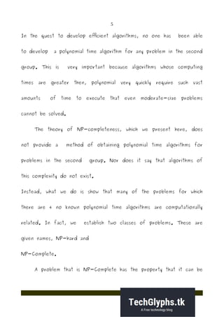
5
In the quest to develop efficient algorithms, no one has been able
to develop a polynomial time algorithm for any problem in the second
group. This is very important because algorithms whose computing
times are greater then, polynomial very quickly require such vast
amounts of time to execute that even moderate-size problems
cannot be solved.
The theory of NP-completeness, which we present here, does
not provide a method of obtaining polynomial time algorithms for
problems in the second group. Nor does it say that algorithms of
this complexity do not exist.
Instead, what we do is show that many of the problems for which
there are 4 no known polynomial time algorithms are computationally
related. In fact, we establish two classes of problems. These are
given names, NP-hard and
NP-Complete.
A problem that is NP-Complete has the property that it can be

6
solved in polynomial time if and only if all other NP-Complete
problems can also be solved in polynomial time. If an NP-hard
problem can be solved in polynomial time, then all NP-Complete
problems can be solved in polynomial time. All NP complete problems
are NP-hard, but some NP-hard problems are not known to be
NP-complete.
Although one can define many distinct problem classes having the
properties stated above for the NP- hard and NP-complete classes,
the classes we study are related to non-deterministic computations.
The relationship of these classes to non deterministic computations
together with
the apparent power of non- determinism lead to the intuitive
conclusion that no NP- complete or NP- hard problem is polynomially
solvable.
3. Briefly explain the concept of trees?

7
A tree is a connected graph without any circuits. The graph in
Fig. , for instance, is a tree. Trees with one, two, three and four
vertices are shown in Fig. . A graph must have at least one vertex,
and therefore so must a tree. Some authors allow the null tree, a
tree without
any vertices. It follows immediately from the definition that a tree
has to be a simple graph, that is, having neither a self-loop nor
parallel edges (because they
both form circuits).
Trees appear in numerous instances. The genealogy of a family is
often represented by means of tree (in fact the term tree comes
from family tree)
A river with its tributaries and subtributaries can be represented by
a tree. The sorting of mail according to zip code and the punched
cards is done according to a tree (called decision tree or sorting
tree).

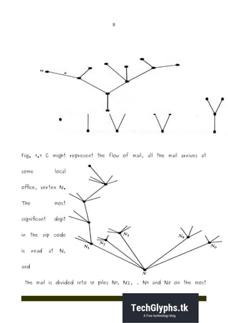
8
Fig. 9.9 C might represent the flow of mail, all the mail arrives at
some local
office, vertex N.
The most
significant digit
in the zip code
is read at N,
and
the mail is divided into 10 piles N1, N2, ... N9 and N0 on the most

9
significant digit. Each pile is further divided into 10 piles according
to second most significant digit, and so on, till the mail is sub
divided into 105 possible piles, each representing a unique five-digit
zip code.
4. Prove that “A tree with n vertices has (n – 1) edges”?
Step (i): If n = 1, then G contains only one vertex and no
edge. So the number of edges in G is n -1 = 1 - 1 = 0.
Step (ii): Induction hypothesis: The statement is true for all trees
with less
than „n vertices.‟
Step (iii): Let us consider a tree with „n vertices.‟
Let „ek be any edge in T whose end vertices are vi and vj.‟
Since T is a tree, there is no other path between vi and vj.
So by removing ek from T, we get a disconnected graph.
Also, T- ek consists of exactly two components(say T1 and T2).
Since T is a tree, there were no circuits in T and so there were no

10
circuits in
T1 and T2. Therefore, T1 and T2 are also trees.
It is clear that |V(T1)| + |V(T2)| = |V(T)| where V(T) denotes the
set of vertices in T.
Also, |V(T1)| and |V(T2)| are les than n.
Therefore, by the induction hypothesis, we have
|E(T1)| = |V(T1)| - 1 and |E(T2)| = |V(T2)| - 1.
Now |E(T)| - 1 = |E(T1)| + |E(T2)| = |V(T1)| - 1 + |V(T2)| - 1
Thus |E(T)| = |V(T1)| + |V(T2)| - 1 = |V(T)| - 1 = n-1.
5. Prove that “A connected graph G is a Euler graph if and only if
it can be decomposed into circuits”
Suppose graph G can be decomposed into circuits; that is, G is a
union of edge-disjoint circuits. Since the degree of every vertex in
a circuit is two, the degree of every vertex in G is even. Hence, G
is an Euler graph.
Conversely, let G be a Euler graph. Consider a vertex v1. There are

11
atleast two edges incident at v1. Let one of these edges be between
v1 and v2. Since vertex v2 is also of even degree, it must have at
least
another edge, say between v2 and v3. Proceeding in this fashion, we
eventually arrive at a vertex that has previously been traversed, thus
forming a circuit . Let us remove from G. All vertices in the
remaining
graph (not necessarily connected) must also be of even degree.
From the remaining graph remove another circuit in exactly the same
way as we removed from G. Continue this process until n o
edges are left.
Hence the theorem.
6. Show that the Clique problem is an NP-complete problem.
The process of establishing a problem as NP-Complete is a
two step process. The first step, which in most of the cases is quite

12
simple, constitutes of guessing possible solutions of the instances, one
instance at a time, of the problem and then verifying whether the
gue ss actually is a solution or not.
The second step involves designing a polynomial-time algorithm which
reduces instances of an already known NP-Complete problem to
instances of the problem, which is intended to be shown as NP-
Complete. However, to begin with, there is a major hurdle in
execution of the second
step. The above technique of reduc tion can not be applied unless
we already have established atleast one problem as NP-Complete.
Therefore, for the first NP-Complete problem, the NP-Completeness
has to be
established in a different manner.
As mentioned earlier, Stephen Cook (1971) established Satisfiability as
the first NP-Complete problem. The proof was based on explicit
reduction of the language of any non-deterministic, polynomial-time

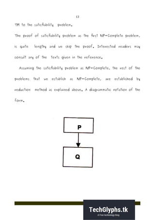
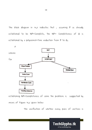
13
TM to the satisfiability problem.
The proof of satisfiability problem as the first NP-Complete problem,
is quite lengthy and we skip the proof. Interested readers may
consult any of the texts given in the reference.
Assuming the satisfiability problem as NP-Complete, the rest of the
problems that we establish as NP-Complete, are established by
reduction method as explained above. A diagrammatic notation of the
form.

14
The block diagram in 14.5 indicates that , assuming P as already
established to be NP-Complete, the NP- Completeness of Q is
established by a polynomial-time reduction from P to Q.
A
scheme
for
establishing NP-Completeness of some the problems is suggested by
means of Figure 14.6 given below:
The verification of whether every pairs of vertices is

15
connected by an edge in E, is done for different pairs of vertices
by a Non-deterministic TM,
i.e., in parallel. Hence, it takes only polynomial time because for each
of n vertices we need to verify atmost n (n + 1) /2 edges, the
maximum number of edges in a graph with n vertices. Next, we show
that 3-CNF-SAT problem can be transformed to clique problem in
polynomial time.
Take an instance of 3-CNF-SAT. An instance of 3CNF-SAT consists
of a set of n clauses, each consisting of exactly 3 literal, each
being either a variable or negated variable. It is satisfiable if we can
choose literals in such a way that:
• Atleast one literal from each clause is chosen
• If literal of form x is chosen, no literal of form x is considered.

16
For
each
of
the
literals, create a graph node, and connect each node to every node
in other clauses, except those with the same variable but different
sign.

Bt0080 fundamentals of algorithms2

More Related Content

Bt0080 fundamentals of algorithms2