Location via proxy:   [ UP ]  
[Report a bug]   [Manage cookies]                
SlideShare a Scribd company logo
Computational Motor
Control Summer School
05: Optimal control for
stochastic systems.
Hirokazu Tanaka
School of Information Science
Japan Institute of Science and Technology
Optimal control for stochastic systems.
In this lecture, we will learn:
• Feedforward and feedback control
• Trial-by-trial variability
• Signal-dependent noise
• Dynamic programming
• Bellman’s optimality equation
• Linear-quadratic-Gaussian (LQG) control
• Optimal feedback control (OFC) model
• Human psychophysics
Feedforward and feedback control.
Feedforward control as a function of time step:
1k k k  x Ax Bu
 k k ku u
Feedback control as a function of state:
 k k ku u x
For a deterministic system, feedforward and feedback control are
equivalent. On the other hand, for a stochastic system, feedforward and
feedback control are NOT equivalent.
Signal-dependent noise: trial-by-trial variability.
van Beers et al. (2004) J Neurophysiol;
Schmidt et al. (1979) Psychol Rev; Jones et al. (2002) J Neurophysiol
Variability in reaching endpoints Variability in force production
   noise
0, 11 , u u
noise noise T
E , Cov       u u u uu
Signal dependent noise
Minimum-variance control predicts smooth trajectory.
Harris & Wolpert (1998) Nature
 1 1n n n n   x Ax Bu
 
   
 
1 1 1
2
2 2 2 1 1
1
0
0
1
1
1 1
1
n
n
k
k
n n n n
n n n n n
n k
k

 

  
 


  
 
  
    

  
x Ax Bu
A x ABu Bu
A x A Bu
  0
1
0
1
E n k
n
n
n
k
k
 


  x A x A Bu
   
T1 T
1
0
T 1
Cov n k n k
n k k
n
k


   
 x A Bu u B A
Minimum-variance control predicts smooth trajectory.
Harris & Wolpert (1998) Nature
   0
1
1
0
E
n
n
k
n k
n
k
f ft t T


 
     x A x A Bu x
   
T1 T T
1
11
110
1
Cov
f f
f f
T
n k n
t t T n
k
t n t k
n k
t
k

  


 
 
 
  
 
  x A Bu u B A
Minimize the variance of final position (quadratic with respect to u)
under constraints (T+1 constraints with respect to u)
This problem can be solved with quadratic programming (quadprog
command).
Minimum-variance control predicts smooth trajectory.
Harris & Wolpert (1998) Nature
Saccade velocity
Reaching and drawing
Minimum-time control predicts Fitts’ law and main sequence.
Tanaka et al. (2006) J Neurophysiol
Faster, but less accurate
300ms 700ms
More precise, but
slower
500ms
Unique movement time
can be determined
 
 
MT ,
T
1
Var (t
( ) E ( )
{ }
)
t tf p
f
t tf p
f
f
p
t f
t f
f
V d
dt t
t
t
S t
t
t



   

 
 
 
 
 

 
 μ x x
u
x
minimization of movement time
final variance constraint
final position constraint
Minimum-time control predicts Fitts’ law and main sequence.
Tanaka et al. (2006) J Neurophysiol
Fitts’ law
Main sequence
Model Experiment
Optimal control: Bellman’s optimality equation.
   
1
0 1 1 0
0
1 1
, , , ;
2 2
N
T T T
N k k k k k N N N
k
J



  u u u x x Q x u Ru x Q x
1k k k  x Ax Bu
Error during
movement
Control cost Endpoint error
Find control signals {u0, u1, …, uN-1} that minimize the cost
function.
Deterministic (i.e., noiseless) dynamics:
Cost function:
Optimal control: Pontryagin’s minimum principle.
State x
Time stepNN-1N-2N-30 1 2 3
u0
u1 u2
u3
uN-3
uN-2
uN-1
x0
x1
x2
x3
xN-3 xN-2
xN-1
xN
   
1
0 1 1 0
0
1 1
, , , ;
2 2
N
T T T
N k k k k k N N N
k
J



  u u u x x Q x u Ru x Q x
The control signals {u0, u1, …, uN-1} are optimized as a whole.
Optimal control: Bellman’s optimality equation.
State x
Time stepNN-1N-2N-30 1 2 3
u0
u1 u2
u3
x0
x1
x2
x3
n n+1 n+2
(cost at state xn at step n)
= (cost of moving xn to xn+1) + (cost at state xn+1 at step 𝑛 + 1)
 1 1n nV  x n nV x
Optimal control: Bellman’s optimality equation.
 
 
 
1 1
1
, , ,
1 1
2 2minn n N
N
T T T
n n k k k k k N N N
k n
V
 


 
   
 
u u u
x x Q x u Ru x Q x
 
 
 
 
 
 
1
1 1
1
1
,
,
,
1
,
,
1
1 1
2 2
1 1 1
2 2 2
min
min min
n N
nn N
n
N
T T T
n n k k k k k N N N
k n
N
T T T T T
n n n n n k k k k k N N N
nk
V
 
 





 
   
 
  
      
  


u u u
u u u
x x Q x u Ru x Q x
x Q x u Ru x Q x u Ru x Q x
   1 1
1
2minn
T T
n n n n n n nV  
 
    u
x Q x u Ru x
 1 1n nV  x
     1 1
1
2minn
T T
n n n n n n n n nV V  
 
    u
x x Q x u Ru x
Solvable example: Linear-Quadratic-Regulator control.
   
     
1 1 1
1
1 1
2 2
1 1
2 2
min
min
T T T
k k k k k k k k k
u
TT T
k k k k k k k k k k
u
V   

 
    
 
      
x x Q x u Ru x S x
x Q x u Ru Ax Bu S Ax Bu
 
 
1 1
1 1
1
0
2
T T T T T T T
k k k k k k k k k k
T T
k k k k
 
 
  
      
  
u Ru u B ABu x A S Bu u B S Ax
u
R B S B u B S Ax
 
1
1 1
T T
k k k k k k

     u R B S B B S Ax L x
Assume that the cost-to-go function has a quadratic form:
 1 1 1 1
1
2
T
k k k kV    x x S x
Substituting this into the Bellman equation gives
Then, by minimizing with respect to u,
A feedback control law is obtained:
Solvable example: Linear-Quadratic-Regulator control.
 
1
1 1
T T
k k k k k k

     u R B S B B S Ax L x
   
11 1
1
1 1
2 2
T
T T
k k k k k k k k
k
V
 

      
x x S x x Q A S BR B A x
 
11 1
1
T T
k k k
 
  S Q A S BR B A
Substituting the control law
into the Bellman equation gives
Therefore a backward recursive equation for the matrix S is obtained.
0
S0
L0
1
S1
L1
2
S2
k-1
Sk-1
Lk-1
k
Sk
Lk
k+1
Sk+1
Lk-2
N-1
SN-1
LN-1
N
SN
LN-2
Solvable example: Linear-Quadratic-Regulator control.
k k k u L x
 
1
1 1
T T
k k k

  L R B S B B S A
 
11 1
1
T T
k k k
 
  S Q A S BR B A
N NS Q
Backward recursion equation for the matrix S:
Feedback control law:
where
with the terminal condition
Therefore, once the matrices {S0, …, SN} and {L0, …, LN-1} are obtained,
the optimal feedback control signals {u0, …, uN-1} can be computed.
Deterministic and stochastic optimal control.
   
1
0 1 1 0
0
1 1
, , , ;
2 2
N
T T T
N k k k k k N N N
k
J



  u u u x x Q x u Ru x Q x
   
1
0 1 1
0 ,
0 0
1 1
ˆ, , , ; E,
2 2
N
T T T
N k k k k k N N N
k
J



 
    
 

w v
u u u x x Q x u Ru x Q x
1k k k
k k
  


x Ax Bu
y Cx
1k k k
k kk
k   



w
v
x Ax Bu
y Cx
Deterministic Optimal Control
Stochastic Optimal Control
Stochastic optimal control combines Kalman filter and feedback control.
ˆk k k u L x
 1
ˆ ˆ ˆk k k k k k    x Ax Bu K y Cx
   
1
0 1 1
0 ,
0 0
1 1
ˆ, , , ; E,
2 2
N
T T T
N k k k k k N N N
k
J



 
    
 

w v
u u u x x Q x u Ru x Q x
1k k k
k kk
k   



w
v
x Ax Bu
y Cx
Stochastic Optimal Control
Optimal state estimation
(Kalman Filter)
Feedback controller
Kalman
filter
Sensory
feedback
Effector
Feedback
controller
Forward
model
Observation
model
y
filter
ˆ u Lx
x
filter
ˆx
prediction
ˆx
prediction
ˆy
Optimal feedback control as a model of motor control.
Todorov & Jordan (2002) Nature Neurosci
   
1
0 1 1
0 ,
0 0
1 1
ˆ, , , ; , E
2 2
N
T T T
N k k k k k N N N
k
J




 
    
 

ω
u u u x x Q x u Ru x Q x
1 k
k
k k k k
k k
   
 
x Ax Bu C
y Hx ω
u
Optimal feedback control as a model of motor control.
Todorov & Jordan (2002) Nature Neurosci; Todorov (2005) Neural Comput
Kalman filter:
 1
ˆ ˆ ˆk k k k k k    x Ax Bu K y Hx
 
 
   
1T T
T T T
1 1 1
1
ˆ T ˆ ˆ
1
;
ˆˆ;
k k k
k k k k k k
T T
k k k k k k



 
   
    
 
    
   
e
x x x
e ω
e e x e
e
K A H H
A K H A CL L C
K H A A BL A BL x
Ω
x
H
Feedback control:
ˆk k k u L x
  
 
   
1
T T T
1 1 1 1
T
1
TT
1 1
;
;
k
N
N
k k k k
k k k k N
k k k k k k
Q

   

 
   
   
    
e
e e e
x x x
x x x
x
L B S B R C S S C B S A
S Q A S A BL S
S A S BL A K H S A K H S 0
Infinite-horizon optimal feedback control.
Phillis (1985) IEEE Trans Auto Contr; Qian et al. (2013) Neural Comput
  ,d dd dt d
d dt d
  

 

  

x Yu G
y Cx
x Bu x
D
A F
 T T T
1 2 0
1
limE E lim
t
t t
J J J dt
t 
 
         
x Ux x Qx u Ru
Stochastic dynamics with signal- and state-dependent noises:
Infinite-horizon cost:
   
.
ˆ ,ˆ
ˆ
ˆd dt d dt   
 
x Ax Bu y
u
x
L
C
x
K
In infinite-horizon optimal feedback control, the Kalman gain (K) and the
feedback gain (L) are time invariant.
Bimanual coordination explained by OFC model.
Dietrichsen (2007) Curr Biol
Two cursor condition One cursor condition
Model
Experiment
Motor adaptation as reoptimization.
Izawa et al. (2008) J Neurosci
Sigmoidal paths
Model Experiment
Field uncertainty
Model Experiment
Movement as a real-time decision making process.
Nashed et al. (2014) J Neurosci
Summary
• Feedforward and feedback control differ in stochastic
dynamics.
• Signal-dependent control noise contributes to trial-by-
trial motor variability.
• Movement accuracy under signal-dependent noise
models human movements.
• Optimal feedback control (OFC) integrates state
estimation and motor control in a single computational
framework.
• A number of psychophysical experiments can be
explained by the OFC model.
References
• Schmidt, R. A., Zelaznik, H., Hawkins, B., Frank, J. S., & Quinn Jr, J. T. (1979). Motor-output variability: a theory for
the accuracy of rapid motor acts. Psychological review, 86(5), 415.
• van Beers, R. J., Haggard, P., & Wolpert, D. M. (2004). The role of execution noise in movement variability. Journal
of Neurophysiology, 91(2), 1050-1063.
• Harris, C. M., & Wolpert, D. M. (1998). Signal-dependent noise determines motor planning. Nature, 394(6695),
780-784.
• Tanaka, H., Krakauer, J. W., & Qian, N. (2006). An optimization principle for determining movement duration.
Journal of neurophysiology, 95(6), 3875-3886.
• Todorov, E., & Jordan, M. I. (2002). Optimal feedback control as a theory of motor coordination. Nature
neuroscience, 5(11), 1226-1235.
• Todorov, E. (2005). Stochastic optimal control and estimation methods adapted to the noise characteristics of the
sensorimotor system. Neural computation, 17(5), 1084-1108.
• Athans, M. (1967). The matrix minimum principle. Information and control, 11(5), 592-606.
• Phillis, Y. A. (1985). Controller design of systems with multiplicative noise. Automatic Control, IEEE Transactions on,
30(10), 1017-1019.
• Qian, N., Jiang, Y., Jiang, Z. P., & Mazzoni, P. (2013). Movement duration, fitts's law, and an infinite-horizon optimal
feedback control model for biological motor systems. Neural computation, 25(3), 697-724.
• Diedrichsen, J. (2007). Optimal task-dependent changes of bimanual feedback control and adaptation. Current
Biology, 17(19), 1675-1679.
• Izawa, J., Rane, T., Donchin, O., & Shadmehr, R. (2008). Motor adaptation as a process of reoptimization. The
Journal of Neuroscience, 28(11), 2883-2891.
• Nashed, J. Y., Crevecoeur, F., & Scott, S. H. (2014). Rapid online selection between multiple motor plans. The
Journal of Neuroscience, 34(5), 1769-1780.
Exercise
• Write a Matlab code of the minimum-variance model for
a trajectory with given initial and final positions.
• Write a Matlab code of the optimal feedback control for
a trajectory with given initial and final positions.
• Investigate how the minimum-variance model and the
optimal feedback model differ.

More Related Content

Computational Motor Control: Optimal Control for Stochastic Systems (JAIST summer course)

  • 1. Computational Motor Control Summer School 05: Optimal control for stochastic systems. Hirokazu Tanaka School of Information Science Japan Institute of Science and Technology
  • 2. Optimal control for stochastic systems. In this lecture, we will learn: • Feedforward and feedback control • Trial-by-trial variability • Signal-dependent noise • Dynamic programming • Bellman’s optimality equation • Linear-quadratic-Gaussian (LQG) control • Optimal feedback control (OFC) model • Human psychophysics
  • 3. Feedforward and feedback control. Feedforward control as a function of time step: 1k k k  x Ax Bu  k k ku u Feedback control as a function of state:  k k ku u x For a deterministic system, feedforward and feedback control are equivalent. On the other hand, for a stochastic system, feedforward and feedback control are NOT equivalent.
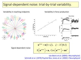
  • 4. Signal-dependent noise: trial-by-trial variability. van Beers et al. (2004) J Neurophysiol; Schmidt et al. (1979) Psychol Rev; Jones et al. (2002) J Neurophysiol Variability in reaching endpoints Variability in force production    noise 0, 11 , u u noise noise T E , Cov       u u u uu Signal dependent noise
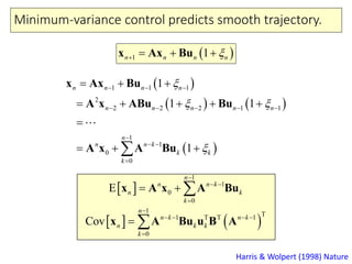
  • 5. Minimum-variance control predicts smooth trajectory. Harris & Wolpert (1998) Nature  1 1n n n n   x Ax Bu         1 1 1 2 2 2 2 1 1 1 0 0 1 1 1 1 1 n n k k n n n n n n n n n n k k                             x Ax Bu A x ABu Bu A x A Bu   0 1 0 1 E n k n n n k k       x A x A Bu     T1 T 1 0 T 1 Cov n k n k n k k n k        x A Bu u B A
  • 6. Minimum-variance control predicts smooth trajectory. Harris & Wolpert (1998) Nature    0 1 1 0 E n n k n k n k f ft t T          x A x A Bu x     T1 T T 1 11 110 1 Cov f f f f T n k n t t T n k t n t k n k t k                    x A Bu u B A Minimize the variance of final position (quadratic with respect to u) under constraints (T+1 constraints with respect to u) This problem can be solved with quadratic programming (quadprog command).
  • 7. Minimum-variance control predicts smooth trajectory. Harris & Wolpert (1998) Nature Saccade velocity Reaching and drawing
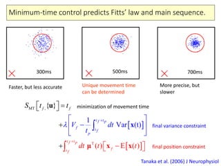
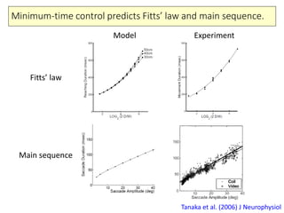
  • 8. Minimum-time control predicts Fitts’ law and main sequence. Tanaka et al. (2006) J Neurophysiol Faster, but less accurate 300ms 700ms More precise, but slower 500ms Unique movement time can be determined     MT , T 1 Var (t ( ) E ( ) { } ) t tf p f t tf p f f p t f t f f V d dt t t t S t t t                       μ x x u x minimization of movement time final variance constraint final position constraint
  • 9. Minimum-time control predicts Fitts’ law and main sequence. Tanaka et al. (2006) J Neurophysiol Fitts’ law Main sequence Model Experiment
  • 10. Optimal control: Bellman’s optimality equation.     1 0 1 1 0 0 1 1 , , , ; 2 2 N T T T N k k k k k N N N k J      u u u x x Q x u Ru x Q x 1k k k  x Ax Bu Error during movement Control cost Endpoint error Find control signals {u0, u1, …, uN-1} that minimize the cost function. Deterministic (i.e., noiseless) dynamics: Cost function:
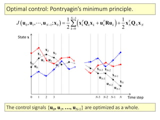
  • 11. Optimal control: Pontryagin’s minimum principle. State x Time stepNN-1N-2N-30 1 2 3 u0 u1 u2 u3 uN-3 uN-2 uN-1 x0 x1 x2 x3 xN-3 xN-2 xN-1 xN     1 0 1 1 0 0 1 1 , , , ; 2 2 N T T T N k k k k k N N N k J      u u u x x Q x u Ru x Q x The control signals {u0, u1, …, uN-1} are optimized as a whole.
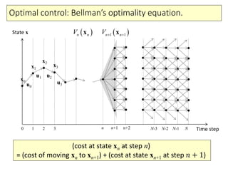
  • 12. Optimal control: Bellman’s optimality equation. State x Time stepNN-1N-2N-30 1 2 3 u0 u1 u2 u3 x0 x1 x2 x3 n n+1 n+2 (cost at state xn at step n) = (cost of moving xn to xn+1) + (cost at state xn+1 at step 𝑛 + 1)  1 1n nV  x n nV x
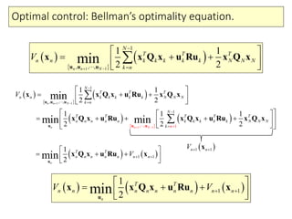
  • 13. Optimal control: Bellman’s optimality equation.       1 1 1 , , , 1 1 2 2minn n N N T T T n n k k k k k N N N k n V             u u u x x Q x u Ru x Q x             1 1 1 1 1 , , , 1 , , 1 1 1 2 2 1 1 1 2 2 2 min min min n N nn N n N T T T n n k k k k k N N N k n N T T T T T n n n n n k k k k k N N N nk V                                 u u u u u u x x Q x u Ru x Q x x Q x u Ru x Q x u Ru x Q x    1 1 1 2minn T T n n n n n n nV         u x Q x u Ru x  1 1n nV  x      1 1 1 2minn T T n n n n n n n n nV V         u x x Q x u Ru x
  • 14. Solvable example: Linear-Quadratic-Regulator control.           1 1 1 1 1 1 2 2 1 1 2 2 min min T T T k k k k k k k k k u TT T k k k k k k k k k k u V                     x x Q x u Ru x S x x Q x u Ru Ax Bu S Ax Bu     1 1 1 1 1 0 2 T T T T T T T k k k k k k k k k k T T k k k k                  u Ru u B ABu x A S Bu u B S Ax u R B S B u B S Ax   1 1 1 T T k k k k k k       u R B S B B S Ax L x Assume that the cost-to-go function has a quadratic form:  1 1 1 1 1 2 T k k k kV    x x S x Substituting this into the Bellman equation gives Then, by minimizing with respect to u, A feedback control law is obtained:
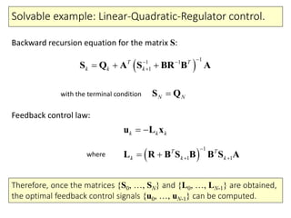
  • 15. Solvable example: Linear-Quadratic-Regulator control.   1 1 1 T T k k k k k k       u R B S B B S Ax L x     11 1 1 1 1 2 2 T T T k k k k k k k k k V           x x S x x Q A S BR B A x   11 1 1 T T k k k     S Q A S BR B A Substituting the control law into the Bellman equation gives Therefore a backward recursive equation for the matrix S is obtained. 0 S0 L0 1 S1 L1 2 S2 k-1 Sk-1 Lk-1 k Sk Lk k+1 Sk+1 Lk-2 N-1 SN-1 LN-1 N SN LN-2
  • 16. Solvable example: Linear-Quadratic-Regulator control. k k k u L x   1 1 1 T T k k k    L R B S B B S A   11 1 1 T T k k k     S Q A S BR B A N NS Q Backward recursion equation for the matrix S: Feedback control law: where with the terminal condition Therefore, once the matrices {S0, …, SN} and {L0, …, LN-1} are obtained, the optimal feedback control signals {u0, …, uN-1} can be computed.
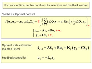
  • 17. Deterministic and stochastic optimal control.     1 0 1 1 0 0 1 1 , , , ; 2 2 N T T T N k k k k k N N N k J      u u u x x Q x u Ru x Q x     1 0 1 1 0 , 0 0 1 1 ˆ, , , ; E, 2 2 N T T T N k k k k k N N N k J              w v u u u x x Q x u Ru x Q x 1k k k k k      x Ax Bu y Cx 1k k k k kk k       w v x Ax Bu y Cx Deterministic Optimal Control Stochastic Optimal Control
  • 18. Stochastic optimal control combines Kalman filter and feedback control. ˆk k k u L x  1 ˆ ˆ ˆk k k k k k    x Ax Bu K y Cx     1 0 1 1 0 , 0 0 1 1 ˆ, , , ; E, 2 2 N T T T N k k k k k N N N k J              w v u u u x x Q x u Ru x Q x 1k k k k kk k       w v x Ax Bu y Cx Stochastic Optimal Control Optimal state estimation (Kalman Filter) Feedback controller
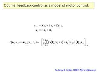
  • 20. Optimal feedback control as a model of motor control. Todorov & Jordan (2002) Nature Neurosci     1 0 1 1 0 , 0 0 1 1 ˆ, , , ; , E 2 2 N T T T N k k k k k N N N k J               ω u u u x x Q x u Ru x Q x 1 k k k k k k k k       x Ax Bu C y Hx ω u
  • 21. Optimal feedback control as a model of motor control. Todorov & Jordan (2002) Nature Neurosci; Todorov (2005) Neural Comput Kalman filter:  1 ˆ ˆ ˆk k k k k k    x Ax Bu K y Hx         1T T T T T 1 1 1 1 ˆ T ˆ ˆ 1 ; ˆˆ; k k k k k k k k k T T k k k k k k                          e x x x e ω e e x e e K A H H A K H A CL L C K H A A BL A BL x Ω x H Feedback control: ˆk k k u L x          1 T T T 1 1 1 1 T 1 TT 1 1 ; ; k N N k k k k k k k k N k k k k k k Q                      e e e e x x x x x x x L B S B R C S S C B S A S Q A S A BL S S A S BL A K H S A K H S 0
  • 22. Infinite-horizon optimal feedback control. Phillis (1985) IEEE Trans Auto Contr; Qian et al. (2013) Neural Comput   ,d dd dt d d dt d            x Yu G y Cx x Bu x D A F  T T T 1 2 0 1 limE E lim t t t J J J dt t              x Ux x Qx u Ru Stochastic dynamics with signal- and state-dependent noises: Infinite-horizon cost:     . ˆ ,ˆ ˆ ˆd dt d dt      x Ax Bu y u x L C x K In infinite-horizon optimal feedback control, the Kalman gain (K) and the feedback gain (L) are time invariant.
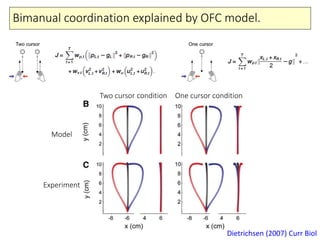
  • 23. Bimanual coordination explained by OFC model. Dietrichsen (2007) Curr Biol Two cursor condition One cursor condition Model Experiment
  • 24. Motor adaptation as reoptimization. Izawa et al. (2008) J Neurosci Sigmoidal paths Model Experiment Field uncertainty Model Experiment
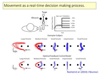
  • 25. Movement as a real-time decision making process. Nashed et al. (2014) J Neurosci
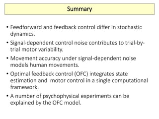
  • 26. Summary • Feedforward and feedback control differ in stochastic dynamics. • Signal-dependent control noise contributes to trial-by- trial motor variability. • Movement accuracy under signal-dependent noise models human movements. • Optimal feedback control (OFC) integrates state estimation and motor control in a single computational framework. • A number of psychophysical experiments can be explained by the OFC model.
  • 27. References • Schmidt, R. A., Zelaznik, H., Hawkins, B., Frank, J. S., & Quinn Jr, J. T. (1979). Motor-output variability: a theory for the accuracy of rapid motor acts. Psychological review, 86(5), 415. • van Beers, R. J., Haggard, P., & Wolpert, D. M. (2004). The role of execution noise in movement variability. Journal of Neurophysiology, 91(2), 1050-1063. • Harris, C. M., & Wolpert, D. M. (1998). Signal-dependent noise determines motor planning. Nature, 394(6695), 780-784. • Tanaka, H., Krakauer, J. W., & Qian, N. (2006). An optimization principle for determining movement duration. Journal of neurophysiology, 95(6), 3875-3886. • Todorov, E., & Jordan, M. I. (2002). Optimal feedback control as a theory of motor coordination. Nature neuroscience, 5(11), 1226-1235. • Todorov, E. (2005). Stochastic optimal control and estimation methods adapted to the noise characteristics of the sensorimotor system. Neural computation, 17(5), 1084-1108. • Athans, M. (1967). The matrix minimum principle. Information and control, 11(5), 592-606. • Phillis, Y. A. (1985). Controller design of systems with multiplicative noise. Automatic Control, IEEE Transactions on, 30(10), 1017-1019. • Qian, N., Jiang, Y., Jiang, Z. P., & Mazzoni, P. (2013). Movement duration, fitts's law, and an infinite-horizon optimal feedback control model for biological motor systems. Neural computation, 25(3), 697-724. • Diedrichsen, J. (2007). Optimal task-dependent changes of bimanual feedback control and adaptation. Current Biology, 17(19), 1675-1679. • Izawa, J., Rane, T., Donchin, O., & Shadmehr, R. (2008). Motor adaptation as a process of reoptimization. The Journal of Neuroscience, 28(11), 2883-2891. • Nashed, J. Y., Crevecoeur, F., & Scott, S. H. (2014). Rapid online selection between multiple motor plans. The Journal of Neuroscience, 34(5), 1769-1780.
  • 28. Exercise • Write a Matlab code of the minimum-variance model for a trajectory with given initial and final positions. • Write a Matlab code of the optimal feedback control for a trajectory with given initial and final positions. • Investigate how the minimum-variance model and the optimal feedback model differ.