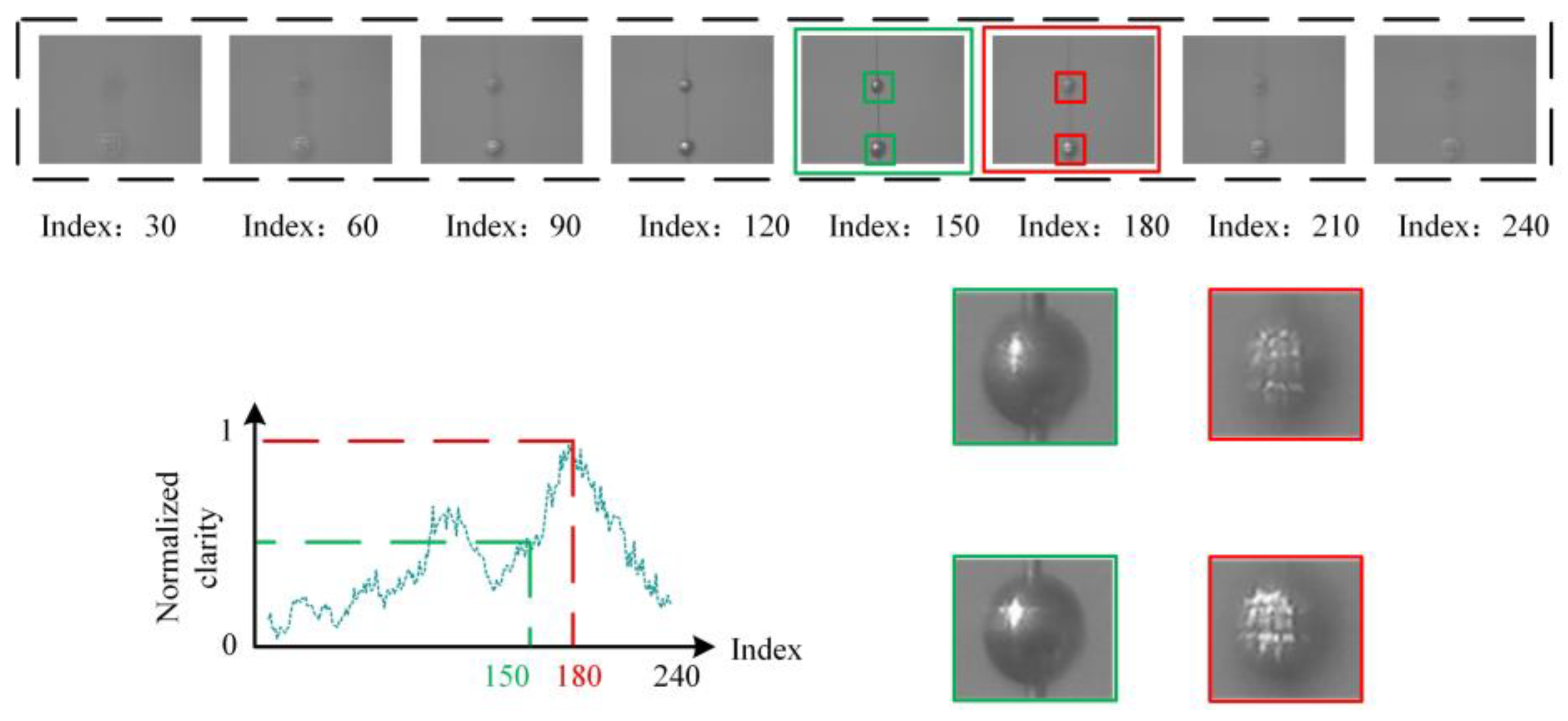
Figure 1.
Misjudgment of light spots. Most evaluation functions tend to misjudge in bokeh scenes, where the red box indicates the misjudged images and the green box represents the actual clear images.
Figure 1.
Misjudgment of light spots. Most evaluation functions tend to misjudge in bokeh scenes, where the red box indicates the misjudged images and the green box represents the actual clear images.
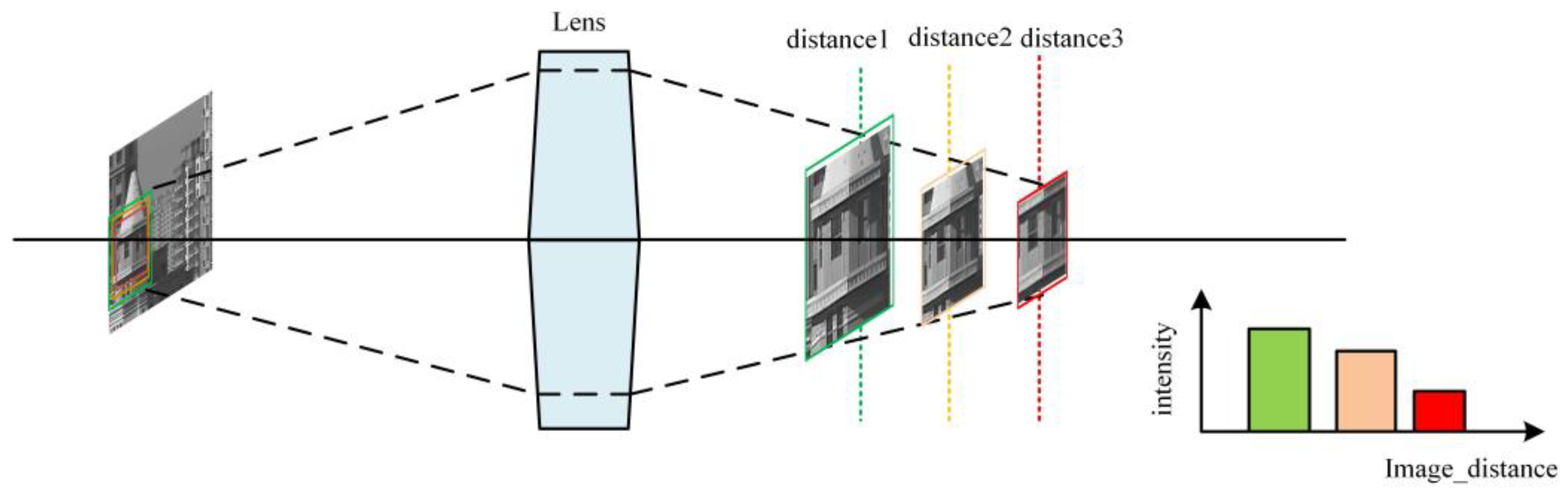
Figure 2.
Different colors correspond to images with different border frames in the figure.
Figure 2.
Different colors correspond to images with different border frames in the figure.
Figure 3.
Lens focus control structure. The camera controls zoom and focus through the motor and uses a potentiometer to record the current position of the lens group.
Figure 3.
Lens focus control structure. The camera controls zoom and focus through the motor and uses a potentiometer to record the current position of the lens group.
Figure 4.
An image stack is a series of images obtained by continuously adjusting the focus value at a fixed focal length, and the stack includes the entire process of the images transitioning from blurry to sharp and back to blurry. Each image stack contains 300 to 400 images.
Figure 4.
An image stack is a series of images obtained by continuously adjusting the focus value at a fixed focal length, and the stack includes the entire process of the images transitioning from blurry to sharp and back to blurry. Each image stack contains 300 to 400 images.
Figure 5.
The dataset was collected under natural lighting conditions from 51 natural scenes, including simple scenes, complex scenes, scenes at a long focal length, and scenes at a short focal length, among other groups of data.
Figure 5.
The dataset was collected under natural lighting conditions from 51 natural scenes, including simple scenes, complex scenes, scenes at a long focal length, and scenes at a short focal length, among other groups of data.
Figure 6.
Sliding window method for data augmentation. The data are expanded by using a sliding window method, while ensuring that the ground truth is evenly distributed across the entire range of categories.
Figure 6.
Sliding window method for data augmentation. The data are expanded by using a sliding window method, while ensuring that the ground truth is evenly distributed across the entire range of categories.
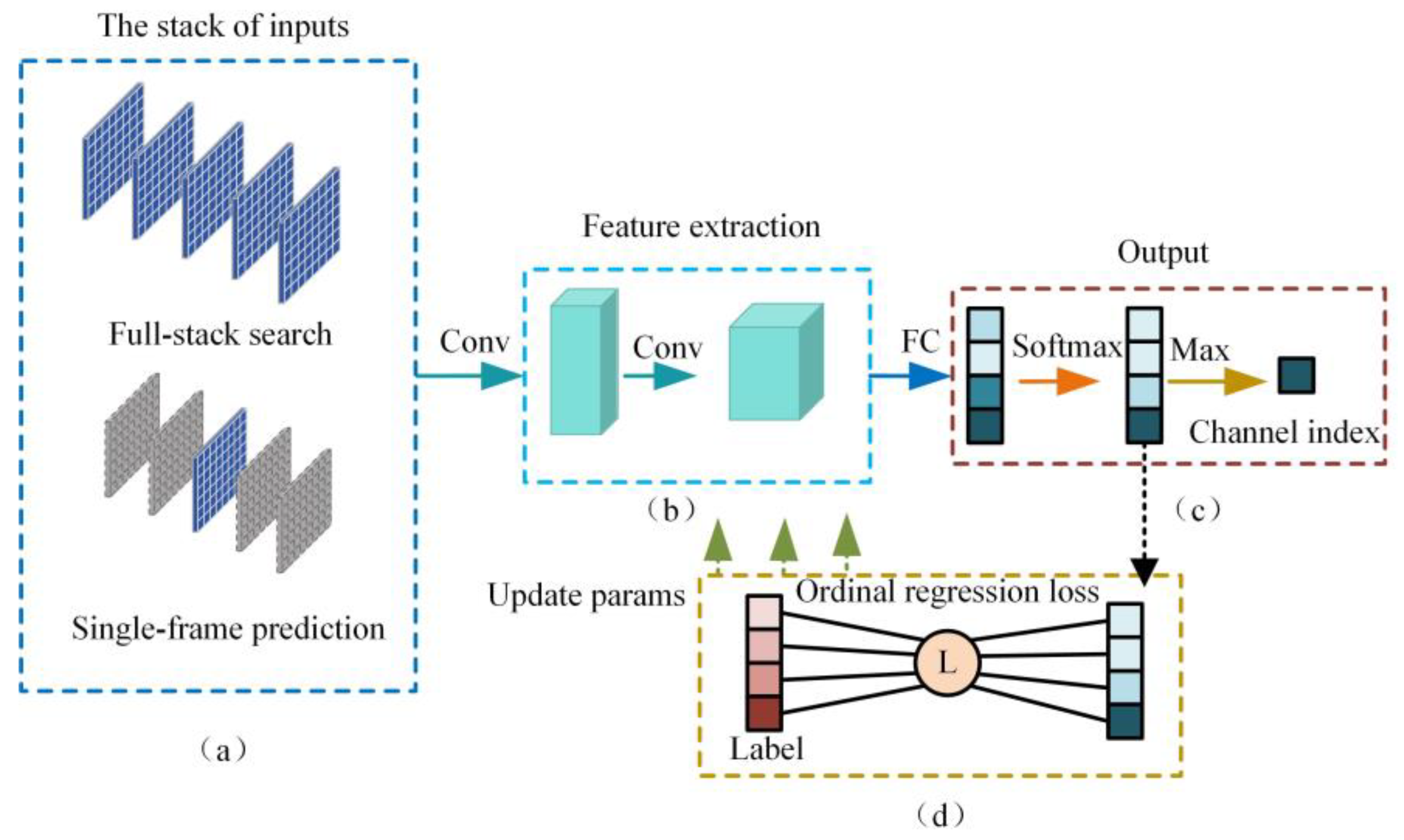
Figure 7.
Full-stack search and single-frame prediction in autofocus. By training the full-stack search and single-frame prediction networks for two different focusing methods through a classification network, the network parameters are optimized using ordinal regression loss, which is different from the classification tasks in the past. (a) First, we modify the network’s input structure to multi-channel input, which is different from the general image processing problem that uses a three-channel RGB image input. We use the channel order to reflect the orderliness of the focus image sequence. The presence of data in the channels is determined based on full-stack search or single-frame prediction. (b) In the feature extraction part, we use existing classification networks to extract feature information from each channel, and classification networks have certain advantages in extracting the main targets in the image. (c) For the network output part, we prefer to use a classification-regression approach, rather than directly outputting the final channel number. The network’s output is the score of multiple channels, and the channel number with the highest score is obtained through softmax and max operations. (d) In the training process, choose the ordinal regression loss function corresponding to the ordinal regression problem. It was found in actual training that if only L1 smooth loss regression loss is used, the network’s convergence speed is very slow.
![Sensors 24 04336 g007]()
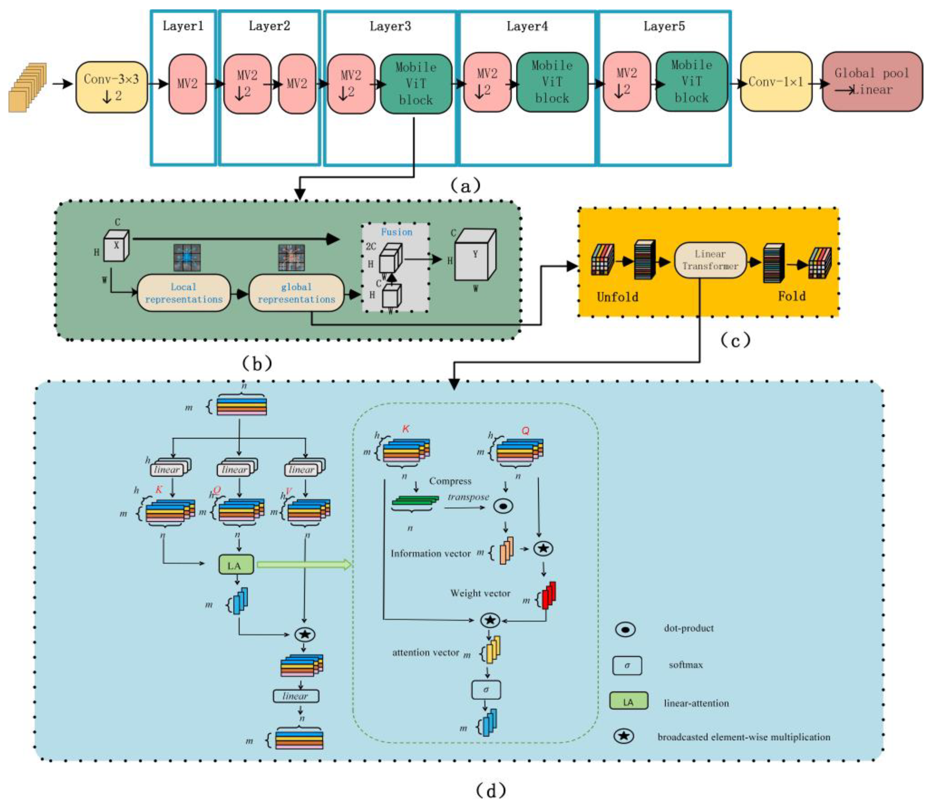
Figure 8.
The structure of the model and linear self-attention. This figure shows the main structure of the classification network we used. We adjusted the network input to multi-channel input and modified the calculation method of the transformer in the global feature representation, introducing a self-attention mechanism with linear complexity, further reducing the computational load of the network. (a) “mv2” represents the mobilenetv2 block, which is an inverted residual structure. The internal structure of the MobileViT block is shown in (b). Its advantage lies in combining the spatial inductive bias of the convolutional network with the global inductive bias of the transformer structure, as shown in (c). The global feature is extracted through the “unfold-linear transformer-fold” method. The unfold operation refers to dividing the two-dimensional image or feature map into multiple small rectangular areas (patches), and then linearizing these areas into a one-dimensional form. The fold operation is the inverse process of unfold, which converts the serialized data back into a two-dimensional form. However, the introduction of the transformer self-attention mechanism increases the computational cost of the network. To this end, we introduced linear attention to reduce the network’s computing power requirements. The specific calculation method of the linear self-attention mechanism is shown in (d). The original self-attention mechanism fuses the attention feature map at the K and Q feature map, which we modified to calculate a set of attention vectors.
![Sensors 24 04336 g008]()
Figure 9.
Soft label loss function. The diagram illustrates the process of calculating a loss function with soft labels for five categories. On the left side, to represent the outputs of the five nodes in the last layer of the neural network. Through softmax, we can enhance the competitive mechanism of the network, allowing categories with higher scores to obtain even higher scores, thus yielding the five outputs to . In terms of label processing, we have abandoned the original one-hot encoding method. Instead, we first calculate the absolute difference between the index of the true value and each label. Based on the calculated absolute difference, we obtain the final soft label through Formula (2).
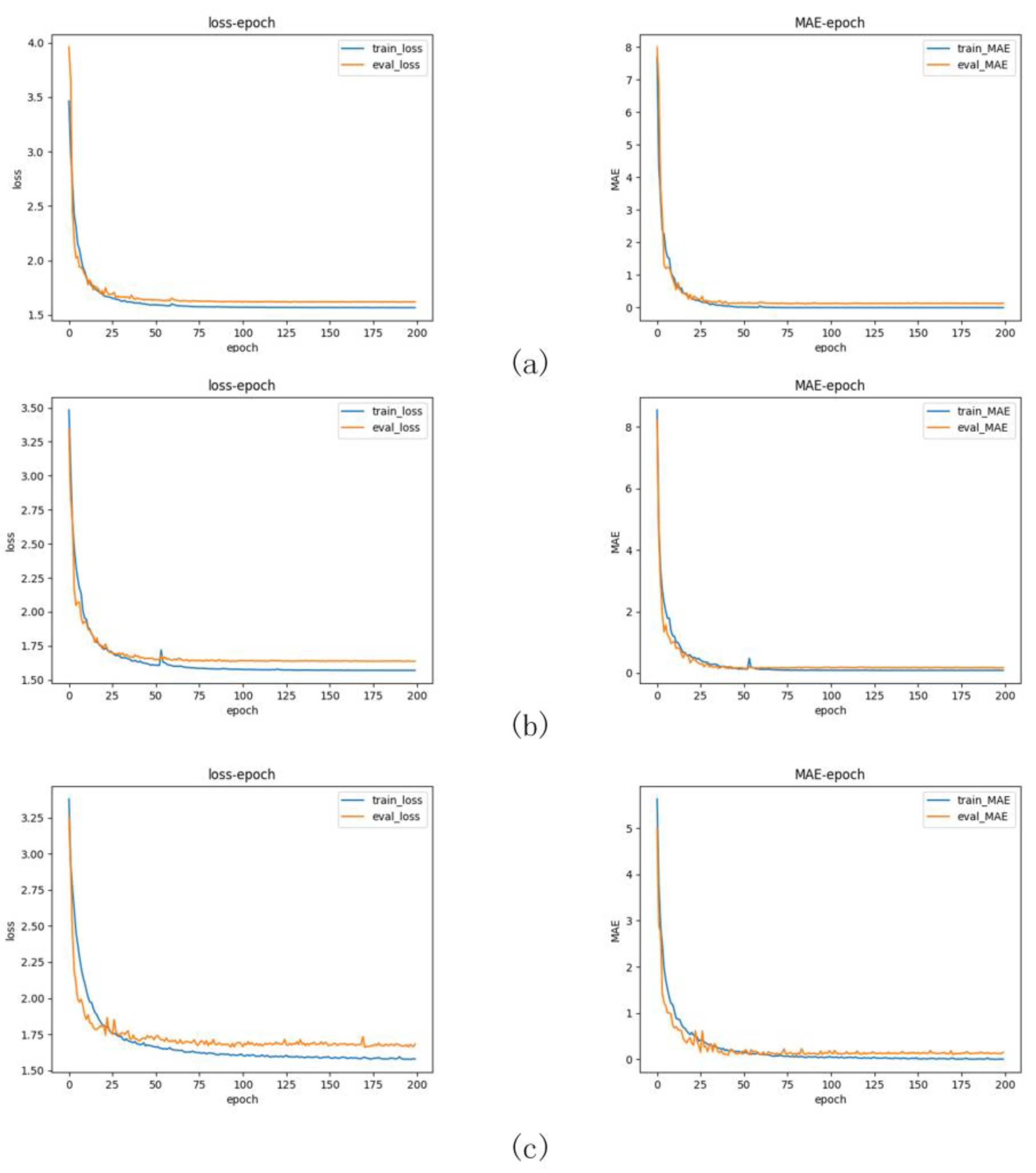
Figure 10.
Training curves and error curves. In the figure above, (a–c) represent the training curves and error curves for the third-best, second-best, and the best results, respectively.
Figure 10.
Training curves and error curves. In the figure above, (a–c) represent the training curves and error curves for the third-best, second-best, and the best results, respectively.
Figure 11.
Parameter amount, error, and GFLOPS bubble chart. In the above figure, the closer the bubble is to the coordinate origin, the better the performance; the smaller the area of the bubble, the less computational resources are required. It can be seen that the comprehensive performances of our algorithm, shufflenetv2-0.5, and shufflenetv2-1.0 are better than those of other models.
Figure 12.
The first column of red boxes in the figure represents the salient target areas in the original image. In the heat map, the more sensitive areas have higher temperatures, which are represented by deeper reds, while the less sensitive areas have lower temperatures, represented by deeper blues. Our network’s region of interest is dynamically changing, and it focuses more on the main subject in the frame compared to other networks.
Figure 13.
Focus results.
Figure 13.
Focus results.
Table 1.
Detailed information and technical specification on the optical lens used.
Table 1.
Detailed information and technical specification on the optical lens used.
| Focal Value Range | Focus Value Range | Exposure Mode | Illumination | Resolution | Number of Scenes | Training Set | Evaluation Set |
|---|
| 160 mm–1500 mm | 200–960 | automatic exposure | natural lighting | 720 × 576 | 51 | 1360 | 680 |
Table 2.
Comparative experiment between full-stack search and traditional evaluation functions.
Table 2.
Comparative experiment between full-stack search and traditional evaluation functions.
| Inxdex | Algorithm | MAE | RMSE | T/ms |
|---|
| 1 | Histogram Entropy [2] | 19.500 | 22.661 | 188 |
| 2 | DCT Reduced Energy Ratio [13] | 16.897 | 19.730 | 248 |
| 3 | Percentile Range [2] | 6.905 | 7.581 | 90 |
| 4 | Wavelet Variance [11] | 6.900 | 8.979 | 352 |
| 5 | Modified DCT [3] | 6.884 | 8.617 | 48 |
| 6 | Wavelet_Ratio [11] | 6.645 | 8.216 | 357 |
| 7 | Gradient Magnitude Variance [4] | 6.586 | 8.135 | 350 |
| 8 | Intensity Coefficient of Variation [2] | 6.546 | 7.360 | 110 |
| 9 | DCT Energy Ratio [2] | 6.499 | 7.348 | 250 |
| 10 | Intensity Variance [2] | 6.419 | 7.322 | 90 |
| 11 | Total Variation L2 [34] | 5.652 | 6.234 | 100 |
| 12 | Gradient Count [2] | 5.634 | 6.279 | 240 |
| 13 | Mean Gradient Magnitude [35] | 5.603 | 6.082 | 345 |
| 14 | Laplacian Variance [4] | 5.110 | 8.148 | 85 |
| 15 | Total Variation L1 [34] | 4.559 | 5.091 | 130 |
| 16 | Wavelet Sum [11] | 3.987 | 5.240 | 340 |
| 17 | Wavelet Weighted [11] | 3.289 | 3.589 | 317 |
| 18 | Diagonal Laplacian [36] | 1.619 | 6.408 | 240 |
| 19 | Ours | 0.094 | 0.201 | 28 |
Table 3.
Comparative experiments with neural networks combining different loss functions.
Table 3.
Comparative experiments with neural networks combining different loss functions.
| Backbone Network | Cross-Entropy | CORAL [29] | Soft Label [31] |
|---|
| MAE | RMSE | T/ms | MAE | RMSE | T/ms | MAE | RMSE | T/ms |
|---|
| Mobilenetv3-l [37] | 1.857 | 3.661 | 18.6 | 0.755 | 1.456 | 18.5 | 0.971 | 1.903 | 19.1 |
| Mobilevit-xs [33] | 0.707 | 1.353 | 25.9 | 0.416 | 0.684 | 25.9 | 0.179 | 0.358 | 25.8 |
| Mobilevit-xxs [33] | 0.588 | 0.823 | 24.2 | 0.567 | 0.803 | 22.6 | 0.201 | 0.397 | 23.7 |
| Shufflenetv2-2.0 [38] | 0.732 | 1.445 | 18.4 | 0.837 | 1.395 | 19.7 | 0.179 | 0.354 | 18.3 |
| Shufflenetv2-1.5 [38] | 0.694 | 1.331 | 18.1 | 0.456 | 0.877 | 19.8 | 0.176 | 0.341 | 18.8 |
| Shufflenetv2-1.0 [38] | 0.572 | 0.823 | 18.7 | 0.232 | 0.435 | 18.6 | 0.172 | 0.327 | 18.4 |
| Shufflenetv2-0.5 [38] | 0.498 | 0.782 | 18.5 | 0.238 | 0.449 | 18.4 | 0.141 | 0.284 | 18.2 |
| Ours | 0.296 | 0.589 | 27.5 | 0.173 | 0.328 | 29.0 | 0.094 | 0.201 | 27.8 |
Table 4.
Comparative table of other ML methods.
Table 4.
Comparative table of other ML methods.
| Method | Cross-Entropy | CORAL [29] | Soft Label [31] |
|---|
| MAE | RMSE | T/ms | MAE | RMSE | T/ms | MAE | RMSE | T/ms |
|---|
| Herrmann [2] | 1.731 | 3.551 | 17.4 | 0.594 | 1.186 | 17.7 | 1.231 | 2.164 | 17.6 |
| Liao [21] | 2.439 | 4.889 | 17.5 | 0.725 | 1.433 | 17.3 | 1.477 | 2.293 | 17.2 |
| Ours | 0.296 | 0.589 | 27.5 | 0.173 | 0.328 | 29.0 | 0.094 | 0.201 | 27.8 |
Table 5.
Comparison table of model computational power and parameter count.
Table 5.
Comparison table of model computational power and parameter count.
| Model | GFLOPS | Parameter/M |
|---|
| Mobilenetv2 [39] | 3.8 | 2.3 |
| Mobilenetv3-l [37] | 2.5 | 4.3 |
| Mobilenetv3-s [37] | 1.0 | 1.6 |
| Mobilevit-xs [33] | 11.4 | 2.0 |
| Mobilevit-xxs [33] (baseline) | 5.9 | 1.0 |
| Shufflenetv2-2.0 [38] | 5.8 | 5.4 |
| Shufflenetv2-1.5 [38] | 3.4 | 2.5 |
| Shufflenetv2-1.0 [38] | 2.1 | 1.3 |
| Shufflenetv2-0.5 [38] | 1.1 | 0.4 |
| Ours | 2.7 | 1.1 |
Table 6.
Comparative table of single-frame prediction.
Table 6.
Comparative table of single-frame prediction.
| Model and Loss Function | MAE | RMSE | T/ms |
|---|
| Mobilenetv2 [39] CORAL [29] | 0.611 | 1.212 | 17.6 |
| Mobilenetv3-s [37] CORAL [29] | 0.811 | 1.561 | 17.4 |
| Mobilenetv3-l [37] CORAL [29] | 0.651 | 1.312 | 18.7 |
| Mobilevit-xs [33] Soft label [31] | 0.246 | 0.478 | 25.7 |
| Mobilevit-xxs [33] Soft label [31] | 0.232 | 0.463 | 23.8 |
| Shufflenetv2-2.0 [38] Soft label [31] | 0.229 | 0.441 | 18.6 |
| Shufflenetv2-1.5 [38] Soft label [31] | 0.223 | 0.432 | 18.4 |
| Shufflenetv2-1.0 [38] Soft label [31] | 0.181 | 0.352 | 18.2 |
| Shufflenetv2-0.5 [38] Soft label [31] | 0.178 | 0.334 | 18.2 |
| Ours Soft label [31] | 0.142 | 0.293 | 27.5 |


