4.1. Dataset and Setup
The Small Aircraft Detection and Tracking Dataset in Ground/Air Infrared Background of the National University of Defense Technology: This dataset is the first comprehensive publicly available dataset specifically designed for detection and recognition purposes in infrared imagery, filling the data gap in the field of infrared object detection and recognition. The dataset consists of 22 data segments collected using unmanned aerial vehicles. Given that our target focuses on the distant infrared imaging of point targets in long-range strike operations, we conducted experiments using only data5, data10, and data21. The details of data 5, data 10 and data 21 are shown in
Table 1. These specific datasets feature long-range imaging, single targets, and ground backgrounds. Data5 encompasses long-term observations with a continuous sequence of three thousand frames, while the other two datasets capture short-term observations with only a few hundred frames. All the images are infrared medium-wave imaging with an image size of 256 × 256.
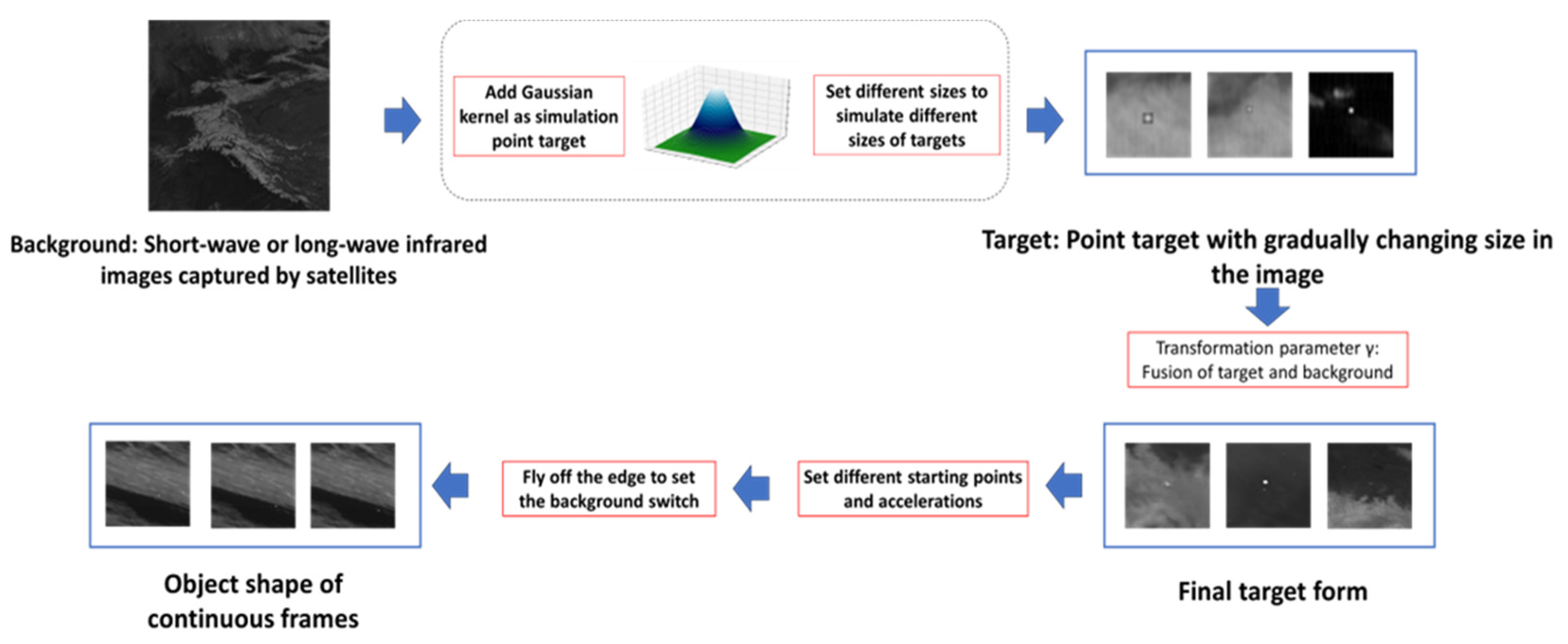
Self-made Infrared Point Target Detection and Tracking Simulation Dataset (MIRPT, Multi-frame InfraRed Point Target): As Infrared Search and Track (IRST) systems are mostly applied to military targets, capturing and tracking targets through high-angle satellite observations, there will be changes in target shape and speed during the movement of military targets due to target ignition or stage separation. However, the target size and speed of the infrared image dataset for small aircraft target detection and tracking mentioned above are very stable. Therefore, in order to test the performance of the algorithm when the target’s shape and speed change, we generated a series of simulated datasets by observing real-time satellite observation data of the ground. These datasets simulate distant observations of targets, which manifest as progressively changing point targets in size within the images. Point target simulation mainly depends on Gaussian kernel generation. The targets are fused with the background, simulating various flight trajectories.
Figure 8 shows the main flow of adding the simulation target to the background image. The simulated data include targets with different velocities, such as cases where vertical ascent does not result in obvious displacement in the image, as well as targets exhibiting acceleration, deceleration, and sudden shifts in position due to abrupt changes in observation angles.
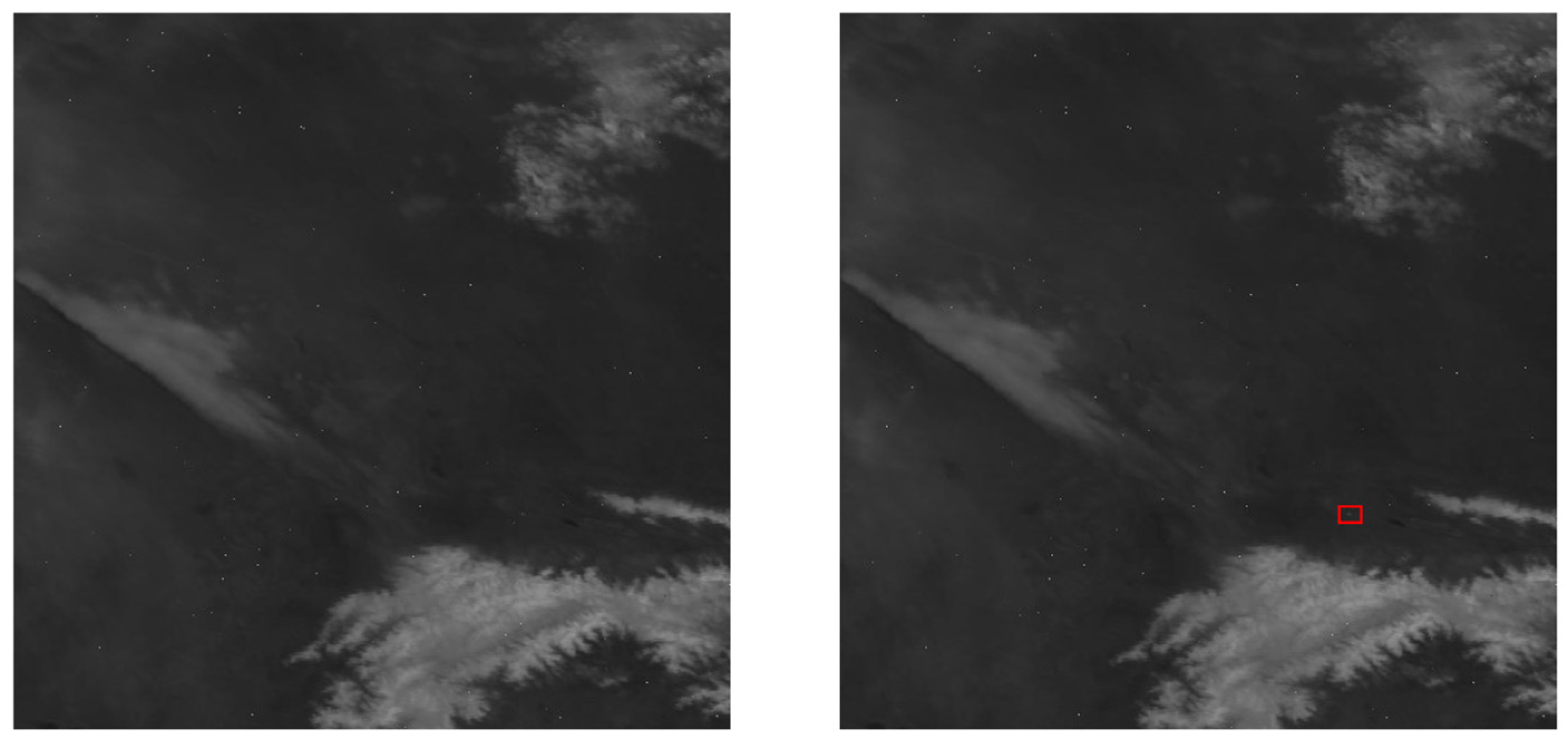
Figure 9 showcases a partial view of the dataset.
There were six data segments in our experiment, among which the infrared image target detection and tracking dataset contains three data segments, and the simulation dataset contains three data segments. Among them, a group of data21 in the infrared image dim and small aircraft target detection and tracking dataset was used as separate test data to verify the robustness of the algorithm in different backgrounds. The other two groups were divided into 2800 training sets and 600 verification sets in proportion. The three sets of data of MIRPT include 5120 training sets and 1020 verification sets. Our network training was conducted using the PyTorch framework on an NVIDIA GTX 2080ti GPU. The experimental settings included a batch size of 16 and 20 epochs. We employed the Adam optimizer with an initial learning rate of 0.01, which decayed by a factor of every 30 epochs. The network parameters and evaluation metrics were referenced from CenterNet.
GT: GT is the abbreviation of ground truth, which is the verified real label provided in the dataset.
TP: the number of detection boxes with IoU > 0.5 (counted only once for each ground truth).
FP: The number of detection boxes with IoU ≤ 0.5 or redundant detection boxes for the same ground truth. AP (average precision): area under the precision–recall (PR) curve.
AR (average recall): The maximum recall of detecting a fixed number of detections per image. In our experiments, the specific value chosen was maxDets = 10.
mAP (mean average precision): this represents the average AP across different categories. Since we only have one category, mAP is equivalent to AP in our case.
Among them, TN and FN are generally not mentioned, because negative samples are not displayed, and there is no problem of distinguishing between true and false. IoU is the abbreviation of Intersection over Union, also known as the overlapping joint ratio. It is a measure used to evaluate the degree of overlap between the bounding box and the real labeling box in a target detection task. IoU measures their overlapping degree by calculating the ratio between the intersection area between the prediction box and the real annotation box and their union area. The value range of IoU is between 0 and 1, and the specific calculation formula is as follows:
TP and FP were used to evaluate each algorithm in our experiment.
In addition, we devised a novel evaluation metric. As our objective involved point target localization, the precise positioning of target keypoints became more crucial than detecting bounding boxes. The new evaluation metric replaced IoU with distance calculation between predicted keypoints and ground truth keypoints. A threshold of 1 was set in this evaluation, yielding more accurate results. In subsequent experiments, we will evaluate the detection performance using both evaluation metrics.
4.3. Comparison with Other Static Detectors
In this section, we present a comparative analysis of our proposed method with other detectors. We evaluate the performance differences between our network and other classic or state-of-the-art object detectors. These methods, both classic and relatively new, include the YOLO series (YOLOv7 [
31], YOLOv8 [
32]), Faster R-CNN [
8], Cascade R-CNN [
33], and infrared-dim and small-target detector with excellent performance. It is worth noting that YOLOv8, similar to our algorithm, is an anchor-free approach. The table below illustrates the comparison between our algorithm, CenterADNet, which incorporates multiple strategic integrations, and these classic and newer object detection algorithms.
It should be mentioned that LESPS [
34] and iSmallnet [
35] need to utilize mask data for training. Our simulated dataset can generate masks independently. Since the infrared small aircraft dataset we used does not have mask annotations, we designed a 3 × 3 bounding box based on the given point target location coordinates to select the target, and then performed threshold segmentation on the local area. After processing, manual verification was conducted. We annotated a total of 3901 images. The mask images are shown in
Figure 10.
From the
Table 6, it can be observed that these algorithms demonstrated relatively high detection accuracy on our simulated dataset. This might be attributed to the high quality of our simulated data, where the targets are comparatively clear. Our baseline algorithm, CenterNet, also exhibited superior performance compared to these algorithms. The performance of our approach was similar to that of the LESPS algorithm in CVPR2023, and our algorithm performed slightly better than LESPS on the simulated dataset.
The third column in the
Table 6 displays a comparison of these algorithms in terms of the number of parameters. It is evident that many excellent algorithms have a significantly lower model complexity compared to our algorithm, and an increase in model complexity can lead to a decrease in computational speed. However, in this paper, to adapt to point targets and use CenterNet to obtain the network’s response to the centrality of point targets, we chose CenterNet as the benchmark network for experiments. As can be seen, our algorithm increased the amount of computation by about 20 M compared to the benchmark network but improved accuracy by more than 5%. Since our algorithm is based on an improvement in CenterNet, the addition of densely connected networks and differential image input layers inevitably led to an increase in the number of parameters and a decrease in inference speed. Nevertheless, in practice, our model can complete calculations for 256 × 256 images in about 1 s during the inference process, making it suitable for most object detection tasks in real-world applications. However, reducing model complexity and integrating lightweight models into hardware remain areas for improvement in our future work.
4.4. Other Experiments
In order to compare with the general infrared-weak small-target detection algorithm, we conducted relevant supplementary experiments using the NUAA-SIRST (SIRST) dataset, which is a general dataset for infrared-weak small targets. Due to the fact that most infrared-weak small-target detection is based on target segmentation, the dataset’s bbox annotation files are somewhat lacking. Therefore, we spent some time re-annotating the dataset with bbox annotations, and the specific modifications to the images are shown in the following
Figure 11: the blue part represents the original data annotation, while the orange part represents the images re-annotated by us.
The SIRST dataset contains a total of 427 images. We divided the dataset into a training set of 341 images and a test set of 86 images according to the data splitting method used in the original dataset, and conducted relevant experiments. We incorporated our method into the experimental results based on those used in iSmallnet. In the
Table 7, the red portion represents the best-performing model, and the bold blue part represents our proposed model. However, since our model requires the use of inter-frame difference images, it does not perform optimally on single-frame small-target detection datasets. Nevertheless, it can be observed that our model achieved performance very close to the optimal model, demonstrating that the network structure we proposed is suitable for feature extraction in the detection of infrared-weak small targets.
4.5. Visualization of Results
In this section, we present specific visualizations of the detection results achieved by our proposed method.
Figure 12 shows the heatmap visualizations of selected data samples. From the images, it is apparent that our proposed method significantly reduced false positives compared to the original approach. The original method still exhibited numerous instances of missed detections, often mistaking the changing speckles between trees as potential targets, leading to a significant decrease in the probability of correctly identifying true targets as keypoints. In contrast, our proposed method exhibited greater stability, although there is a certain degree of positional displacement. However, the majority of these displacements fell within the centroid distance verification metric we proposed.
Figure 13 illustrates the performance of our method compared to the original approach in terms of accuracy. These experimental results represent the average performance obtained from the five datasets we used. The graph clearly shows that our method not only achieved higher accuracy but also demonstrated greater stability compared to the original algorithm. The original algorithm exhibited some sudden fluctuations in the numerical values. Despite conducting multiple experiments, this issue persisted. We hypothesize that this is because the original detector does not leverage temporal information from multiple frames. As a result, it is susceptible to slight variations in single-frame images, which can significantly impact detection results.
In addition, to validate the robustness of our algorithm, we conducted a separate set of tests on images with a completely new background. The dataset is data21, mentioned in
Section 4.1. This set of data contains 500 test images. The target in the picture is still a point target, but the brightness of the target is quite different, and the imaging is blurred. Previous tests involved splitting a complete dataset into training and testing sets, where the backgrounds were relatively consistent, making the detection task less challenging. To assess our algorithm’s performance, we introduced a new set of data with a completely different background.
Figure 14 showcases the detection results of our algorithm on the images with the new background. It is evident from the graph that both algorithms generate numerous false positives when facing a new background. However, our algorithm significantly reduces the number of false positives compared to the original algorithm. Additionally, the original algorithm tends to lose track of the targets in many frames, while our algorithm demonstrates the ability to track the targets over a longer period.


 ,
, 


