The Influence of Geostatistical Prior Modeling on the Solution of DCT-Based Bayesian Inversion: A Case Study from Chicken Creek Catchment

Abstract

Low frequency loop-loop electromagnetic induction (EMI) is a widely-used geophysical measurement method to rapidly measure in situ the apparent electrical conductivity (ECa) of variably-saturated soils. Here, we couple Bayesian inversion of a quasi-two-dimensional electromagnetic (EM) model with image compression via the discrete cosine transform (DCT) for subsurface electrical conductivity (EC) imaging. The subsurface EC distributions are obtained from multi-configuration EMI data measured with a CMD-Explorer sensor along two transects in the Chicken Creek catchment (Brandenburg, Germany). Dipole-dipole electrical resistivity tomography (ERT) data are used to benchmark the inferred EC fields of both transects. We are especially concerned with the impact of the DCT truncation method on the accuracy and reliability of the inversely-estimated EC images. We contrast the results of two different truncation approaches for model parametrization. The first scenario considers an arbitrary selection of the dominant DCT coefficients and their prior distributions (a commonly-used approach), while the second methodology benefits from geostatistical simulation of the EMI data pseudosection. This study demonstrates that DCT truncation based on geostatistical simulations facilitates a robust selection of the dominant DCT coefficients and their prior ranges, resulting in more accurate subsurface EC imaging from multi-configuration EMI data. Results based on geostatistical prior modeling present an excellent agreement between the EMI- and ERT-derived EC fields of the Chicken Creek catchment.

1. Introduction

Noninvasive geophysical methods have found widespread application for subsurface characterizations at spatial scales spanning the root zone to regional aquifers [1,2,3]. This near-surface environment is highly heterogeneous and comprised of a rich biodiversity of living organisms, which interact with rock, soil, and water to regulate the natural habitat and determine the availability of nutrients and other life-sustaining resources. Electromagnetic (EM) geophysical methods provide a wealth of information about the subsurface electrical properties and are particularly well-suited for in situ measurement and monitoring of variables such as electrical conductivity ($\sigma$ or EC (mS/m)) and permittivity [1,4,5,6,7]. These data are of great value to water quality and water resource studies and key input to (hydro)geophysical models that simulate the flow, storage, and distribution of fluids in the subsurface [3,7,8].

Electromagnetic induction (EMI) is a relatively inexpensive and easy to use geophysical measurement method for measuring in situ the subsurface apparent electrical conductivity (${\sigma }_{\mathrm{a}}$ or ECa (mS/m)) [9,10,11,12]. The EMI reading is a proxy for the weighted average electrical conductivity of the soil column bounded on top by the ground surface and at the bottom by the maximum penetration depth of the instrument. This depth is determined by coil orientation, inter-coil spacing (the so-called offset), and frequency, listed in order of decreasing importance [13]. As the EMI instrument does not require ground contact, it does not suffer from electrical coupling problems, thereby facilitating a rapid data acquisition and mapping of the electrical properties of variably-saturated soils [7,8,12,14].

Several different deterministic inversions have been developed to model a layered distribution of the subsurface EC from EMI data. Mester et al. [13] and Jadoon et al. [15] applied two-layered inversion strategies for subsurface imaging from multi-configuration EMI data. Other work by Dafflon et al. [4] used grid-based inversion of EMI data to determine permafrost properties and the spatial variability of the active soil layer. Triantafilis and Monteiro Santos [16] introduced the inversion software of EM4Soil for subsurface EC imaging. Most recently, Christiansen et al. [17] applied the non-linear inversion algorithm of Auken et al. [18] (AarhusInv) on EMI data for archaeological prospecting. Notwithstanding the attractive features of multi-layered EMI inversion, this approach increases manifold the number of unknown EC values. This equates to a high-dimensional inverse problem, which may result in an under-determined problem because of the limited information of the EMI data (sensitivity of the return signal depends in large part on inter-coil spacing and coil orientation).

Multi-layered inversions of the EMI data using deterministic approaches are typically interpreted as a single-best solution. This warrants a Bayesian formulation of the EMI inverse problem and demands use of a stochastic search method [19,20] to quantify properly the uncertainty of the estimated values. An example of such Bayesian approach was presented by Moghadas et al. [7] who used Markov chain Monte Carlo (MCMC) simulation with the DREAM${}_{\left(\mathrm{ZS}\right)}$ algorithm [21] to characterize spatiotemporal variations in soil water content from time-lapse EMI data. This state-of-the-art MCMC method has found widespread use in many different fields of study and simplifies considerably the application of Bayesian inference to parameter-rich and/or CPU-intensive system models [22,23]. Recently, Moghadas [24] demonstrated the efficiency of incorporating discrete cosine transform (DCT) with the Bayesian inversion of EMI data via numerical simulations. The proposed methodology is computationally efficient since the model compression based on DCT allows for relatively fast convergence of the inverse problem. The use of adequate prior information for DCT-based Bayesian inference is important for accurate subsurface imaging and reducing the parameter uncertainty estimation. In this respect, geostatistical prior modeling simplifies the inverse problem and substantially improves subsurface characterizations [24,25].

In this paper, we apply the methodology of Moghadas [24] and use a quasi-two-dimensional EM model to mimic the EMI measurement process along a transect in pursuit of the subsurface EC distribution. This necessitates discretization of the soil domain of the transect in a large number of grid cells. The EC of each grid cell is then determined by fitting the quasi-two-dimensional EM model to a collection of EMI data measured at equidistant intervals along the transect. We use Bayesian inference to characterize the subsurface EC distribution from a multi-configuration CMD-Explorer sensor. The measurements were realized along two transects at the Chicken Creek (Hühnerwasser) catchment (Brandenburg, Germany). Electrical resistivity tomography (ERT) surveys were also separately carried out to image in situ the EC distribution and benchmark the inferred EC fields of both transects. The DCT of Ahmed et al. [26] was used to reduce considerably the dimensionality of multi-layered EMI inversion. To explore the impact of the DCT truncation method on the accuracy of the inverse solution, we consider two different approaches for model compression. The first approach considers an arbitrary selection of the dominant DCT coefficients and their prior ranges, while the second methodology benefits from geostatistical simulations of ECa images for truncation.

2. Study Area and Measurements

This study focuses on the Chicken Creek artificial catchment located in the Lusatian Lake District in Brandenburg, Germany. This six-hectare catchment is the result of a post-mining restoration project and was commissioned between May 2004 and September 2005 to promote interdisciplinary ecosystem research. Figure 1a presents an areal overview of the artificial catchment. The immediate subsurface is comprised of three layers with contrasting textures and variable depths. The 1–3-m base soil is followed by a Tertiary clay layer (aquiclude) of 1–3 m in thickness and sand layer (aquifer) of down to 3.5 m in depth on the top of the domain. The large and sudden variations in layer thicknesses are the result of denudation, weathering, ecologic, and biogeochemical processes [27].

EMI surveys were carried out along two transects (labeled 1 and 2 in Figure 1b) using CMD-Explorer (GF Instruments, s.r.o., Brno, Czech Republic). This multi-coil instrument operates at a frequency of 10 kHz and contains three receiver coils at a distance of 1.48, 2.82, and 4.49 m from the transmitter. This equates to an effective penetration depth of 1.1, 2.1, and 3.3 m, respectively, in vertical coplanar (VCP) mode. In horizontal coplanar (HCP) mode, the penetration depths increase to values of 2.3, 4.2, and 6.7 m for the reported offsets of 1.48, 2.82, and 4.49 m. The two perpendicular transects of 134 and 120 m cover a large segment of the Chicken Creek catchment with important variations in subsurface properties. The EMI data were collected at regular intervals of 2 m, which equates to a total of $K=68$ and $K=61$ measurement locations for Transects 1 and 2, respectively. The use of two antenna modes and three offsets leads to six measured ECa data at each observation location. The corresponding ECa measurements of both antenna modes, ${\tilde{\sigma }}_{\mathrm{a}}^{\mathrm{HCP}}$ and ${\tilde{\sigma }}_{\mathrm{a}}^{\mathrm{VCP}}$, at the K measurement locations are grouped together in $2K$-vectors, ${\tilde{\mathsf{\sigma }}}_{\mathrm{a}}$ for each transect. The apparent resistivity of the subsurface was measured with the multi-channel ERT 4-Point-Light 10-W system of Lippmann Geophysical Instruments (Schaufling, Germany) using a dipole-dipole array with electrode separation of 1 m. Then, the apparent resistivity data of each transect were inverted with the RES2DINV software package of Loke et al. [29]. The so-obtained subsurface resistivity models were converted into an image of the EC of each transect down to a 6-m depth.

3. Modeling Framework

3.1. EMI Forward Model

In this study, we used a so-called full EM forward model and mimicked the EMI measurement process at our experimental field site using numerical solutions of the Maxwell equations [30,31]. This model is valid under low and high induction numbers and simulates exactly the ECa for horizontal and vertical coplanar antenna modes, ${\sigma }_{\mathrm{a}}^{\mathrm{HCP}}$ and ${\sigma }_{\mathrm{a}}^{\mathrm{VCP}}$, respectively [32]. To simplify comparison with the measured ECa data, we grouped together the simulated values of ${\sigma }_{\mathrm{a}}^{\mathrm{HCP}}$ and ${\sigma }_{\mathrm{a}}^{\mathrm{VCP}}$ at each lateral measurement point, x, of each transect in $2K$-vectors, ${\mathsf{\sigma }}_{\mathrm{a}}$. To solve the forward model, we assumed a soil column comprised of N layers at every measurement point along each transect. Note that we considered a one-dimensional stratified earth model, but we formulated the modeling procedure in a quasi-two-dimensional framework to enhance the efficiency of the problem. We assumed a measurement depth of 6 m and discretized the subsurface domain of both transects using a structured grid. This discretization amounted to a $N\times M$ matrix with $N=20$ rows (soil layers) and $M=68$ or $M=61$ columns (lateral position) for Transects 1 and 2, respectively. This necessitated specification of 1360 and 1220 different values of the EC and amounts to a CPU-demanding and high-dimensional parameter estimation problem. The next section discusses a Fourier-related transform with real numbers, the DCT-II, to simplify considerably the EMI inverse problem.

3.2. Discrete Cosine Transform

Lets us embed our EM field in a x-z coordinate system with increasing values of x from left to right across the transect and with $z=0$ at the top and $z>0$ at the bottom of the soil profile. We need to characterize efficiently the electrical field of this soil domain composed of $N\times M$ grid cells. Hereto, we used the Type-II DCT of Ahmed et al. [26], which expresses a finite sequence of data points as a sum of cosine functions oscillating at different frequencies. For a uniformly-discretized domain of $n\times m$ cells, the DCT-II is given by:

$$G(i,j)={\alpha }_i{\alpha }_j\sum _{z=1}^n\sum _{x=1}^{m}S(z,x)cos\left(\frac{(i-1)\pi (2z-1)}{2n}\right)cos\left(\frac{(j-1)\pi (2x-1)}{2m}\right),$$

(1)

where $i>0$ and $j>0$ signify the row and column number of the $n\times m$ DCT coefficient matrix, $\mathbf{G}$, and the $n\times m$ matrix $\mathbf{S}$ stores center values of the EC of each DCT-II grid cell. The scalars ${\alpha }_i$ and ${\alpha }_j$ are defined as follows:

$${\alpha }_i=\left\{\begin{array}{cc}\frac{1}{\sqrt{n}}\hfill & \mathrm{if}i=1\hfill \\ \sqrt{\frac{2}{n}}\hfill & \mathrm{if}2\le i\le n\hfill \end{array}\right.{\alpha }_j=\left\{\begin{array}{cc}\frac{1}{\sqrt{m}}\hfill & \mathrm{if}j=1\hfill \\ \sqrt{\frac{2}{m}}\hfill & \mathrm{if}2\le j\le m.\hfill \end{array}\right.$$

(2)

Equation (1) turns the $n\times m$ matrix $\mathbf{S}$ with EC values into a similar size matrix, $\mathbf{G}$, of DCT coefficients. The top-left element of this matrix, $G(1,1)$, corresponds to the zero-frequency component, whereas entries in subsequent columns and rows of matrix G store the DCT coefficients of increasingly higher spatial frequencies in the horizontal and vertical direction, respectively. This space-to-frequency transformation concentrates the spatial detail of the EC field in the lower frequency components of the matrix $\mathbf{G}$. Those entries are conveniently organized in a d-vector, $\mathsf{\theta }=\left\{G\right(1,1),\dots ,G(i,j\left)\right\}$, with $i>1$ and $j>1$, and the remaining high frequency DCT coefficients in the bottom-right part of matrix $\mathbf{G}$ are set to zero. As $d\ll nm$, this approach simplifies considerably geophysical inversion and subsurface characterization [23,25,33]. This approach necessitates use of the Type-III DCT, simply called inverse DCT, to turn the matrix $\mathbf{G}$ with low-frequency components estimated from the measured EMI data and stored in vector $\mathsf{\theta }$ into an $n\times m$ map of EC values. This inferred map of EC values is then interpolated to the $N\times M$ grid of the EM forward model.

The DCT has important practical advantages for EMI data analysis. A sparse formulation in the frequency domain not only reduces drastically the computational requirements for subsurface characterization, but allows also for the simultaneous use of all measured ECa data of each transect. In other words, the quasi-two-dimensional DCT-based Bayesian inference involves all ECa values along each transect in an over-determined inversion framework. This stabilizes the inverse problem and promotes smoothness of the inferred EC map. Yet, the use of DCT model compression may complicate somewhat the definition of a reasonable prior distribution for the frequency components of matrix $\mathbf{G}$. The full-EM model with DCT compression uses as input argument the d-vector $\mathsf{\theta }$ with low frequency DCT components and returns a $2K$-vector with simulated ECa values for the HCP and VCP antenna modes at the K measurement locations of each transect. The order of the elements of ${\mathsf{\sigma }}_{\mathrm{a}}$ matches exactly their measured ECa values, ${\tilde{\mathsf{\sigma }}}_{\mathrm{a}}$ for each transect. The $2K$-vector of ECa residuals, $\mathbf{e}\left(\mathsf{\theta }\right)$, for each transect can now be written as:

$$\mathbf{e}\left(\mathsf{\theta }\right)={\tilde{\mathsf{\sigma }}}_{\mathrm{a}}-{\mathsf{\sigma }}_{\mathrm{a}}\left(\mathsf{\theta }\right)=\{e_1\left(\mathsf{\theta }\right),\dots ,e_{2K}\left(\mathsf{\theta }\right)\}.$$

(3)

3.3. Structured Grids and DCT Parametrization

Now, we have defined the different building blocks of our coupled EM model and DCT compression framework, and we are left with the definition of the structured grid that is used to characterize the EC field of the subsurface. This boils down to setting values for n, the number of soil layers, and m, the number of blocks in the lateral direction, x of our DCT-II grid. The larger the values of n and m, the denser the discretized DCT-II grid, and consequently, the higher the resolution will be of the resolved EC field. The use of a dense grid, however, places a premium on computational resources and may not necessarily lead to a well-defined inverse solution. The use of a coarse grid, on the other hand, reduces considerably the CPU time of the EM forward model and, thus, computational costs for parameter estimation, yet the resolution may not be sufficient to warrant reconstruction of small-scale variations in the EC. This trade-off between image resolution and image uncertainty complicates the choice for an adequate value of n and m.

In this paper, we juxtapose the results of two different truncation approaches. These two methods, hereafter referred to as Truncation-I and Truncation-II, are illustrated graphically in Figure 2. The first grid in Figure 2a is comprised of $n=12$ soil layers and $m=60$ cells in the lateral position. Without prior information, the common truncation approach is to consider the upper left corner (a box or a triangle) of the $n\times m$ matrix as model parameters (an arbitrary selection of the DCT coefficients), since most of the information regarding the DCT is stored in this part of the domain [22]. Instead of a computationally-expensive search in the full parameter space of dimension $n\times m$, it is assumed that the properties of the model can be described with a much lower dimension with the remaining elements being zero. As a first approach (Truncation-I), we thus characterized the EC values of the regular grid of 720 cells using the $d=45$ frequencies from the sub-matrix $\mathbf{G}(1:3,1:15)$ of the $n\times m$ DCT coefficient matrix $\mathbf{G}$. The remaining coefficients of $\mathbf{G}$ were set to zero. Note that the 45 low-frequency components of the Truncation-I were arbitrarily selected without using geostatistical simulations.

In contrast to the commonly-applied selection of low frequencies (Truncation-I), we here explored the merits of an alternative truncation method (Truncation-II) using geostatistical simulations to select the dominant DCT coefficients. This approach draws inspiration from Lochbuhler et al. [25] and takes much better advantage of measured EMI data in the selection of the location and number of low-frequency DCT coefficients from $\mathbf{G}$ and the determination of their prior ranges. To this end, we use the ECa image measured with CMD Explorer as the training data image for geostatistical simulation with the DeeSse code [34,35]. This patented code is an improved implementation of the direct sampling technique proposed by Mariethoz et al. [34] and uses multiple-point statistical (MPS) simulation to extract efficiently key features and patterns from a training image (TI). The reader is referred to Moghadas [24] for further details regarding the DeeSse settings for DCT parametrization.

The ECa images were created by plotting the ECa values of each measurement point against their effective penetration depth. These one-dimensional ECa data were then stitched together to produce apparent electrical conductivity pseudosections down to the maximum penetration depth of the EMI sensor. The inferred ECa data pseudosections were further interpolated in both vertical and horizontal directions, providing a better presentation of the subsurface variations of the ECa data. Note that the interpolation procedure was performed to improve the perception about the subsurface features. The ECa images can also be used as TIs without interpolation, since the MPS algorithm requires a conceptual subsurface model (a general impression of the subsurface features) as a training image. Lochbuhler et al. [25] demonstrated that a large number of realizations (= 1000) from a TI should be generated to ensure the stable and reliable simulations. Consequently, we used DeeSse software to generate 1000 different realizations of the TI of Transects 1 and 2, respectively, for efficient model parametrization.

Each TI realization was then transformed to the frequency domain using Equations (1) and (2). The low-frequency DCT coefficients of matrix $\mathbf{G}$ were determined from this ensemble of frequency domain realizations [24]. The original set of low-frequency DCT coefficients was downsampled considering the occupancy probability of the DCT coefficients (derived from the 1000 realizations) and trades-off model complexity and uncertainty. This means, after determination of all low-frequency DCT coefficients from thousand of MPS realizations, the occupancy probability of each coefficient was calculated conceiving how many times a specific coefficient appeared as a dominant DCT coefficient. Afterwards, the unknown model parameters were determined by considering a trade-off between the occupancy probability and the number of coefficients [24]. Figure 2b summarizes the different steps of Truncation-II and depicts graphically the final selection of the low-frequency coefficients from $\mathbf{G}$ for the structured DCT-grid composed of $n=12$ soil layers and $m=60$ lateral cells.

The EMI measurement frequency and DCT-II compression framework exert control on the properties of the grid and the selection of the DCT coefficients. With a low measurement frequency of about 10 kHz (diffusive regime), the vertical resolution of the EMI data is somewhat limited. As a consequence, we used a coarse structure of $n=12$ soil layers for both DCT-II grids due the diffusive regime of the data. What is more, the DCT-II compression concentrates the low-frequency coefficients of our rectangular subsurface domain in the lateral position. This simply echoes a much larger transect length than measurement depth. Therefore, the selection of the DCT coefficients of $\mathbf{G}$ is biased in the horizontal direction.

4. Probabilistic Inversion

We used Bayesian analysis to infer the d-vector $\mathsf{\theta }$ of low-frequency components of matrix $\mathbf{G}$ from ECa transect measurements, ${\tilde{\mathsf{\sigma }}}_{\mathrm{a}}$, derived from CMD-Explorer. Bayesian inference treats the unknown values of $\mathsf{\theta }$ as probabilistic variables with joint posterior probability density function, $p(\mathsf{\theta }|{\tilde{\mathsf{\sigma }}}_{\mathrm{a}})$, which expresses exactly parameter uncertainty. This multivariate distribution, the so-called posterior distribution, is the consequence of a prior distribution, $p(\mathsf{\theta })$, which captures our initial degree of beliefs in the values of the model parameters, and a likelihood function, $L(\mathsf{\theta }|{\tilde{\mathsf{\sigma }}}_{\mathrm{a}})\equiv p({\tilde{\mathsf{\sigma }}}_{\mathrm{a}}|\mathsf{\theta })$, which quantifies via probability theory the level of confidence (= conditional belief) in the parameter values, $\mathsf{\theta }$, given the observed data, ${\tilde{\mathsf{\sigma }}}_{\mathrm{a}}$, alone. Bayes’ theorem expresses mathematically, and in a simple formula, the fundamental relationship between the prior, conditional, and posterior (= updated) beliefs of the parameters:

$$p(\mathsf{\theta }|{\tilde{\mathsf{\sigma }}}_{\mathrm{a}})=\frac{p(\mathsf{\theta })p({\tilde{\mathsf{\sigma }}}_{\mathrm{a}}|\mathsf{\theta })}{{\int }_{\mathbf{\Theta }}p(\mathsf{\theta })p({\tilde{\mathsf{\sigma }}}_{\mathrm{a}}|\mathsf{\theta })}\propto p(\mathsf{\theta })L(\mathsf{\theta }|{\tilde{\mathsf{\sigma }}}_{\mathrm{a}}),$$

(4)

where the normalizing constant, $p({\tilde{\mathsf{\sigma }}}_{\mathrm{a}})={\int }_{\mathbf{\Theta }}p(\mathsf{\theta })L(\mathsf{\theta }|{\tilde{\mathsf{\sigma }}}_{\mathrm{a}})$, reduces $p(\mathsf{\theta }|{\tilde{\mathsf{\sigma }}}_{\mathrm{a}})$ to a probability density function with integral of unity over the prior (feasible) parameter space, $\mathsf{\theta }\in \mathbf{\Theta }\subseteq {\mathbb{R}}^d$. The denominator, also called evidence or marginal likelihood, is relevant for hypothesis testing via model selection [36], but of no particular importance for parameter estimation, as all statistical inferences about the parameters $\mathsf{\theta }$ of the EM forward model can be made from the unnormalized posterior distribution, $p(\mathsf{\theta }|{\tilde{\mathsf{\sigma }}}_{\mathrm{a}})\propto p(\mathsf{\theta })L(\mathsf{\theta }|{\tilde{\mathsf{\sigma }}}_{\mathrm{a}})$.

4.1. Prior Distribution

The parameter vector, $\mathsf{\theta }$, is made up of the d lowest frequency components of the DCT coefficient matrix, $\mathbf{G}$ in Equation (1). To define prior distribution for $\mathsf{\theta }$ (in the frequency domain), it is important to first define the minimum (${\sigma }_{\min }$) and maximum (${\sigma }_{\max }$) EC values in the space domain. We adjusted these parameters such that ${\sigma }_{\min }=1$ and ${\sigma }_{\max }=100$ mS/m. The values of ${\sigma }_{\min }$ and ${\sigma }_{\max }$ were selected in such a way to cover a relatively large conductivity range. In the absence of detailed knowledge about the values of $\mathsf{\theta }$, we assumed a d-variate uniform prior distribution for the low-frequency DCT coefficients. For Truncation-I, the upper and lower bounds of each DCT coefficient in $p\left(\mathsf{\theta }\right)$ were determined iteratively using the scaling methodology of Linde and Vrugt [22]. The outcome of this are ranges of $p\left(\mathsf{\theta }\right)$, which, after inverse transform of matrix G with low-frequency components of $\mathsf{\theta }$, can produce EC values for each grid cell between ${\sigma }_{\min }=1$ and ${\sigma }_{\max }=100$ mS/m.

For Truncation-II, the upper and lower bounds of the DCT coefficients in $p\left(\mathsf{\theta }\right)$ were inferred from the thousand TI realizations [24]. These bounds were scaled in such a way that the inverse DCT of $\mathbf{G}(1,1)$ was between ${\sigma }_{\min }=1$ and ${\sigma }_{\max }=100$ mS/m (see Figure 2b). It is important to note that an ECa data pseudosection is not representative of the real subsurface EC values, but it provides a conceptual model of the subsurface EC variations. As a consequence, EMI measured ECa image of each transect offers a great potential to be used as a TI for the MPS simulations. As previously mentioned, the prior information of Truncation-II was inferred form geostatistical realizations of the ECa data pseudosection, providing realistic uncertainty estimations. During the Bayesian inversion, images with EC values that fell outside the stipulated range of $1-100$ mS/m were assigned a negligible likelihood for both truncation strategies. This will help the search algorithm delineate and discard unproductive areas of the parameter (frequency) space.

4.2. Likelihood Function

The likelihood function, $L(\mathsf{\theta }|{\tilde{\mathsf{\sigma }}}_{\mathrm{a}})$, measures in a probabilistic sense the distance between the measured and modeled ECa values simulated with the EM-model and DCT-II compression using the low-frequency DCT coefficients, $\mathsf{\theta }$. If we make the convenient assumption that the ECa residuals, $\mathbf{e}\left(\mathsf{\theta }\right)=\{e_1\left(\mathsf{\theta }\right),\dots ,e_{2K}\left(\mathsf{\theta }\right)\}$, in Equation (3) are independent, zero-mean normally distributed with constant variance, then a Gaussian likelihood suffices:

$$L(\mathsf{\theta }|{\tilde{\mathsf{\sigma }}}_{\mathrm{a}})\propto {\left(\sum _{k=1}^{2K}{e}_k^2\left(\mathsf{\theta }\right)\right)}^{-K}$$

(5)

to find the optimal DCT coefficients, ${\mathsf{\theta }}^{*}$. This is equivalent to minimizing the root mean squared error (RMSE) of the $2K$-vector, $\mathbf{e}\left(\mathsf{\theta }\right)$, of ECa residuals:

$${\mathsf{\theta }}^{*}=\arg \underset{\mathsf{\theta }\in \mathbf{\Theta }}{min}\mathrm{RMSE}\left(\mathsf{\theta }\right),$$

(6)

where:

$$\mathrm{RMSE}=\sqrt{\frac{1}{2K}\sum _{k=1}^{2K}{\left[{\tilde{\sigma }}_{\mathrm{a},k}-{\sigma }_{\mathrm{a},k}\left(\mathsf{\theta }\right)\right]}^2}=\sqrt{\frac{1}{2K}\sum _{k=1}^{2K}{e}_k^2\left(\mathsf{\theta }\right)}.$$

(7)

The assumptions of independence and normality are convenient in applying statistical theory, but may not be borne out by actual series of ECa residuals, which may exhibit (among others) bias, skew, a non-constant variance, and complex serial dependencies. We therefore relaxed the common assumptions of normality and serial independence, and resorted to the generalized likelihood function (GLF) of Schoups and Vrugt [37]:

$$L(\mathsf{\theta }|{\tilde{\mathsf{\sigma }}}_{\mathrm{a}},\widehat{\mathsf{\sigma }},\beta ,\xi ,{\mathbf{\Phi }}_p)\simeq \prod _{k=1}^{2K}\frac{2}{{\widehat{\sigma }}_k}\left(\frac{{\sigma }_{\xi }{\omega }_{\beta }}{\xi +{\xi }^{-1}}\right)exp\left\{-c_{\beta }{\left|\frac{{\tau }_k(\mathsf{\theta },{\mathbf{\Phi }}_p)}{{\xi }^{sgn\left({\tau }_k(\mathsf{\theta },{\mathbf{\Phi }}_p)\right)}}\right|}^{2/(1+\beta )}\right\},$$

(8)

where $\widehat{\mathsf{\sigma }}=\{{\widehat{\sigma }}_1,\dots ,{\widehat{\sigma }}_{2K}\}$ signifies a $2K$-vector of standard deviations of the ECa measurement error, ${\tau }_k(\mathsf{\theta },{\mathbf{\Phi }}_p)={\mu }_{\xi }+{\sigma }_{\xi }{\epsilon }_k(\mathsf{\theta },{\mathbf{\Phi }}_p)$ is the unstandardized value of the $k^{\mathrm{th}}$ decorrelated residual, ${\epsilon }_k(\mathsf{\theta },{\mathbf{\Phi }}_p)$, $sgn\left(a\right)$ denotes the signum function, and the scalars, ${\omega }_{\beta }$, $c_{\beta }$, ${\mu }_{\xi }$, and ${\sigma }_{\xi }$ are a function of the kurtosis parameter, $\beta$, and skewness parameter, $\xi$ using Equations (A1)–(A5) in Appendix A. The underlying density function of Equation (8) is symmetric for $\xi =1$, positively skewed for $\xi >1$, and negatively skewed for $\xi <1$. For a symmetric density, that is $\xi =1$, a value of $\beta =-1$ results in a uniform distribution, $\beta =0$ produces a normal distribution, and $\beta =1$ portrays a double-exponential or Laplace distribution.

The vector of decorrelated residuals, $\mathsf{\epsilon }(\mathsf{\theta },{\mathbf{\Phi }}_p)=\{{\epsilon }_1(\mathsf{\theta },{\mathbf{\Phi }}_p),\dots ,{\epsilon }_{2K}(\mathsf{\theta },{\mathbf{\Phi }}_p)\}$, is computed from:

$${\mathbf{\Phi }}_p\left(B\right)e_k\left(\mathsf{\theta }\right)={\widehat{\sigma }}_k{\epsilon }_k,$$

(9)

where B represents the backward shift (“backshift”) operator, that is $B^r{e}_k\left(\mathsf{\theta }\right)=e_{k-r}\left(\mathsf{\theta }\right)$, and:

$${\mathbf{\Phi }}_p\left(B\right)=1-\sum _{u=1}^p{\varphi }_u{B}^u,$$

(10)

is an autoregressive polynomial with p coefficients, ${\mathbf{\Phi }}_p=\{{\varphi }_1,\dots ,{\varphi }_p\}$, where ${\varphi }_u\in [-1,1]$ and $u=\{1,\dots ,p\}$. Note that $B^1{e}_k\left(\mathsf{\theta }\right)=e_{k-1}\left(\mathsf{\theta }\right)$ and $B^2{e}_k\left(\mathsf{\theta }\right)=B\left(B{e}_k\left(\mathsf{\theta }\right)\right)=e_{k-2}\left(\mathsf{\theta }\right)$, and so forth.

The q random variables, $\mathit{\alpha }=\{\beta ,\xi ,{\mathbf{\Phi }}_p\}$, are fundamental to the probabilistic description of the ECa residuals, but are not of particular interest themselves. These so-called nuisance variables can be estimated along with the model parameters, $\mathsf{\theta }$. This latter approach allows the GLF to describe accurately the skew, kurtosis, and serial dependencies of the ECa residuals, $\mathbf{e}\left(\mathsf{\theta }\right)$ in Equation (3). If the measurement error standard deviations, $\widehat{\mathsf{\sigma }}=\{{\widehat{\sigma }}_1,\dots ,{\widehat{\sigma }}_{2K}\}$, of the ECa observations, ${\tilde{\mathsf{\sigma }}}_{\mathrm{a}}=\{{\tilde{\sigma }}_{\mathrm{a},1},\dots ,{\tilde{\sigma }}_{\mathrm{a},2K}\}$, are known a-priori, then the formulation of Equation (8) suffices. Otherwise, we can relate ${\widehat{\sigma }}_k$ to the measured ECa data, ${\tilde{\sigma }}_{\mathrm{a},k}$, as follows:

$${\widehat{\sigma }}_k=s_0+s_1{\tilde{\sigma }}_{\mathrm{a},k}$$

(11)

where $s_0>0$ and $s_1\in [0,1]$ are two unknown coefficients that define the intercept and slope of the measurement error function (heteroscedasticity). The values of $s_0$ and $s_1$ were then estimated along with the other nuisance variables of the GLF; thus, $\mathit{\alpha }=\{s_0,s_1,\beta ,\xi ,{\mathbf{\Phi }}_p\}$.

Interested readers are referred to Vrugt and Massoud [38] for a detailed step-by-step derivation of Equation (8). It suffices here to say that the Gaussian likelihood assumes residual errors are to be independent and to be described by a normal probability distribution with a mean of zero and a constant variance. The GLF can describe properly non-Gaussian residuals with non-constant variance, varying degrees of kurtosis and skewness, and serial correlation at different temporal and/or spatial lags. In other words, the GLF considers more realistic assumptions for error residuals, which necessitate estimating the nuisance variables along with the model parameters. For the present application of the GLF, we assume that an AR(1) model suffices to describe the serial correlation of the ECa residuals. This leaves us with $q=5$ nuisance variables, $\mathit{\alpha }=\{s_0,s_1,\beta ,\xi ,{\varphi }_1\}$, whose values are inferred jointly with the d low-frequency DCT coefficients of $\mathsf{\theta }$ using the multivariate prior distribution on $\{\mathsf{\theta },\mathit{\alpha }\}$ and the likelihood function of Equation (8). The uniform prior uncertainty ranges of the nuisance variables were set as $0<s_0<0.1$ S/m, $0<s_1<1$, $-1<\beta <1$, $0.1<\xi <10$, and $0<{\varphi }_1<1$, as suggested by Schoups and Vrugt [37].

4.3. Posterior Distribution

Now, we have defined the prior distribution, $p(\mathsf{\theta },\mathit{\alpha })$, and the likelihood function, $L(\mathsf{\theta },\mathit{\alpha }|{\tilde{\mathsf{\sigma }}}_{\mathrm{a}})$, and we are left with inference of the posterior distribution, which summarizes our updated knowledge on the parameters, $\mathsf{\theta }$, and nuisance variables, $\mathit{\alpha }$. Here, we used MCMC simulation with the multi-try differential adaptive metropolis, or MT-DREAM${}_{\left(\mathrm{ZS}\right)}$, algorithm of Laloy and Vrugt [39] to approximate the target distribution, $p(\mathsf{\theta },\mathit{\alpha }|{\tilde{\mathsf{\sigma }}}_{\mathrm{a}})$. A detailed description of the MT-DREAM${}_{\left(\mathrm{ZS}\right)}$ algorithm appears in Laloy and Vrugt [39]. Benchmark experiments have shown MT-DREAM${}_{\left(\mathrm{ZS}\right)}$’s ability to sample rapidly and accurately high-dimensional target distributions [22,25,40,41]. Convergence of the sampled chains was monitored using the $\widehat{R}$ statistic of Gelman and Rubin [42], which compares the within-chain and between-chain variance of each parameter of $\mathsf{\theta }$. Convergence can be declared if ${\widehat{R}}_j\le 1.2$ for each parameter, otherwise a larger number of generations is required [43].

As previously mentioned, the Bayesian inference summarizes the uncertainty by treating the unknown values as probabilistic variables with a posterior distribution that includes the 95% confidence interval. The maximum-a-posteriori (MAP) estimate is equivalent to the posterior solution with the maximum probability. Comparison between the MAP solution and the posterior mean (MEAN) helps to investigate the accuracy and robustness of the inverse problem. In this respect, a well-posed Bayesian inference captures our initial degree of beliefs in the unknown parameters and the likelihood function with posterior mean that remains in close vicinity of the MAP solution. The 95% confidence interval also allows for exploring the uncertainty of the parameter estimations. Here, we summarize and present the results of our MCMC simulations in MAP, MEAN, and 95% confidence intervals.

5. Results and Discussion

5.1. EMI and ERT Data

Figure 3 summarizes the inversely-estimated ERT models along with the ECa images. The top panel presents images of the EC of Transects 1 (left) and 2 (right) derived from the inversion of the measured ERT resistivity data using the RES2DINV program. The bottom panel displays the ECa pseudosections of both transects. A common x-axis is used to simplify comparison of the ERT inverted models and ECa images.

The ERT profile of Transect 1 in Figure 3a demonstrated the presence of several horizontally layered bands with contrasting EC values. These bands meandered up and down the profile from left to right across the transect with EC values that increase with soil depth. The top layer (in red) consisted of a sand material with EC values that range between 1 and 20 mS/m. The depth of this layer increased from about 2 m at $x=0$ to about 4 m at the end of the first transect. Immediately underneath this sand layer, we found a finer textured material composed of four bands with very different EC values. The top part of the clay layer constituted a small yellow band of about 30 cm in thickness with values of $\sigma =28$ mS/m. This was followed by a green band of about 80 cm in thickness with EC values between 40 and 50 mS/m and a magenta band of about 20 cm with $55<\sigma <60$ mS/m. The bottom part of the clay layer with values of $60<\sigma <80$ mS/m completed the profile. These four different EC bands traversed up and down the profile, but with a trend towards larger depths for increasing values of x along the transect. The four distinctive bands within the clay layer expressed variations in moisture content, possibly guided by changes in soil texture. The EC image of the first transect measured with ERT confirmed the presence of lateral variations in the thickness and depth of the sand and clay layer. Such variations are in agreement with Figure 1a.

The EC image of the second transect in Figure 3b was qualitatively similar to that of Transect 1 with the exception that the different bands with contrasting EC values did not meander as much across the transect. Indeed, the sand layer exhibited a rather constant depth of about 2.5 m. The finer textured, clay, layer underneath was of rather constant thickness, but demonstrated an enlarged area of $25<\sigma <60$ mS/m in between the two edges with high EC values of about 90 mS/m. Nevertheless, the ERT resistivity data of the second transect suggested a uniform horizontal layering of the top sand layer and bottom clay layer. This finding is consistent with the location of Transect 2 in Figure 1a.

The ECa data of Transect 1 exhibited a compelling lateral pattern with different colored ECa bands that dipped to larger depths for increasing values of x along the transect. The measured ECa data of the second transect, however, demonstrated a more uniform layering with a constant depth of the red top layer and clay layer immediately underneath. For the time being, we conclude that the ECa pseudosections from our EMI surveys are in qualitative agreement with the EC measurements derived from ERT imaging. This motivated our use of the ECa images as TI for geostatistical simulation using direct sampling with DeeSse software.

5.2. MPS Simulation Results

Truncation-II used as training datasets the ECa images of Transects 1 and 2 displayed in Figure 3c,d. Figure 4a,b displays five images of the ensemble of 1000 ECa realizations derived from geostatistical simulation of the TI of Transects 1 and 2, respectively. These images were derived from direct sampling with DeeSse software. Frequency domain transformation of the 1000 DeeSse realizations resulted in 238 low-frequency DCT coefficients for Transect 1, and 322 low-frequency DCT coefficients for Transect 2. Figure 4c,d highlights with gray color the corresponding cells of the $n\times m$ structured DCT grid for both transects. The original set of low-frequency DCT coefficients was downsampled to 47 (Transect 1) and 44 (Transect 2) cells, which are displayed in gray in Figure 4e,f.

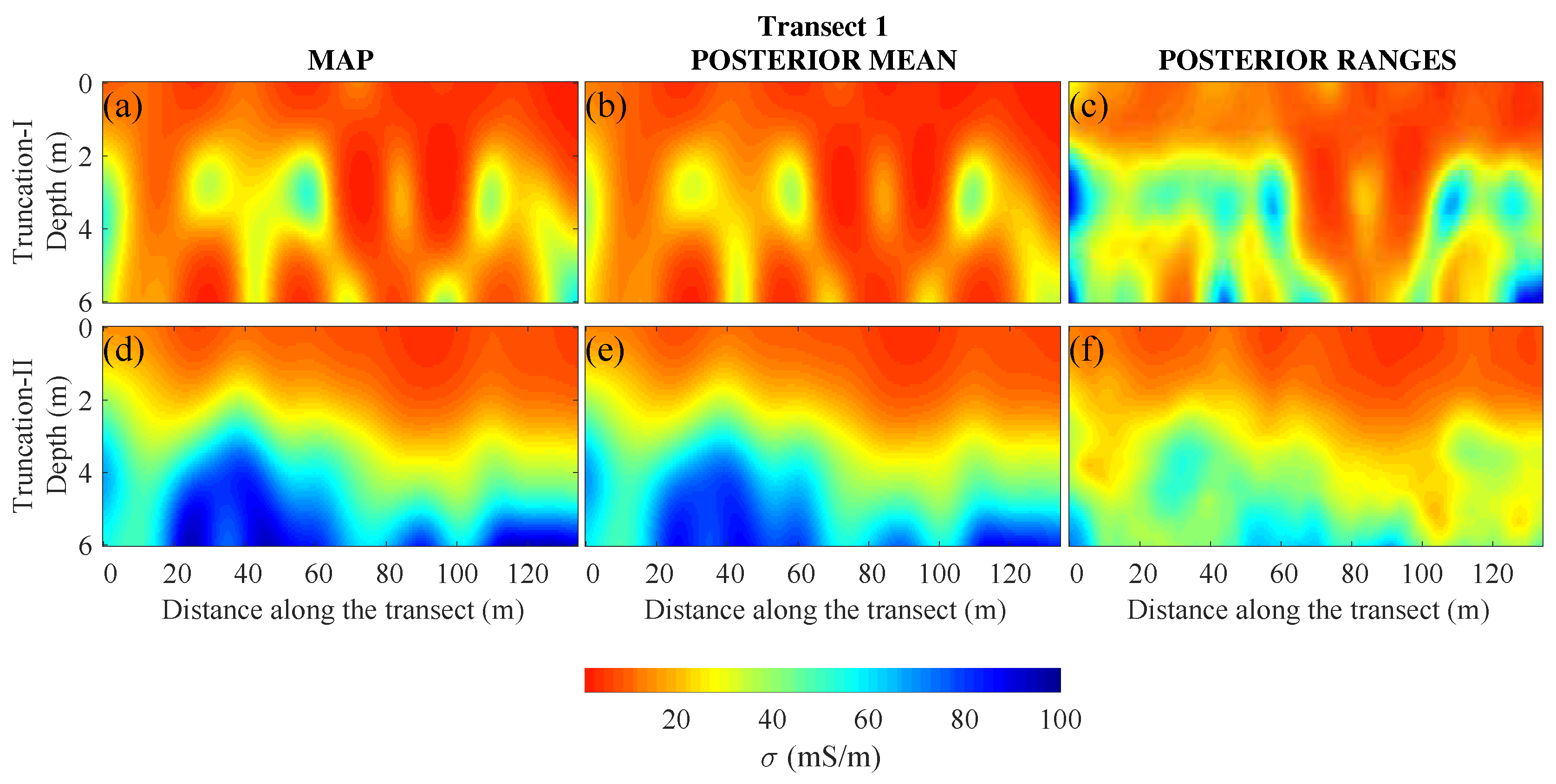
5.3. Transect 1: Inversion Results

Figure 5 presents the results of MCMC simulation with the MT-DREAM${}_{\left(\mathrm{ZS}\right)}$ algorithm using the GLF of Equation (8) with Truncation-I (top row) and Truncation-II (bottom row), respectively. The left and middle columns display the EC field of the MAP and the MEAN solutions, respectively, whereas the right column displays the 95% confidence intervals of the EC values derived from the posterior samples. The results in Figure 5 highlight several important findings. In the first place, notice the close agreement between the MAP and posterior MEAN images of Truncation-I and II, respectively. This was not an unexpected result, but provided evidence for the claim that the DCT-based inverse problem was well-posed with posterior EC models that remained in close vicinity of the MAP image. Second, the MAP and MEAN images derived from Truncation-I appeared rather inferior. The two images were made up of large red spots with a spatial pattern of the EC values that was absent and incommensurate with the horizontal layering so evidently present in the ERT-derived EC image of Transect 1. Third, the MAP and MEAN images derived from Truncation-II matched closely with its ERT measured counterpart of Transect 1. Indeed, both maps demonstrated the presence of layering and were comprised of several bands with distinctly different EC values. These EC values generally increased with depth in the profile. Last, but not least, the 95% confidence intervals of the EC image appeared rather small close to the surface and tended to increase deeper in the soil profile.

To better understand the EC images derived from the EMI data, please consider Figure 6, which presents histograms of the posterior RMSE values of Truncation-I (light gray) and Truncation-II (dark gray) sampled by the MT-DREAM${}_{\left(\mathrm{ZS}\right)}$ algorithm. We calculated the RMSE between the measured and modeled ECa values for the posterior samples, providing posterior RMSE of the different MCMC inversion runs. The posterior EC images derived from Truncation-I exhibited RMSE values between 10 and 16 mS/m. These values were substantially larger than their counterparts of about 2 mS/m derived from EMI data inversion with Truncation-II. This difference in RMSE values explained the rather poor EC images of Truncation-I and provided support for the use of ECa training images to guide the selection of a suitable set of low-frequency DCT coefficients in pursuit of a sparse model parameterization. As Truncation I and II had in common many different DCT coefficients (see Figure 4e,f), the use of an inadequate prior distribution may certainly explain the rather inferior results of Truncation-I for Transect 1. What is more, the GLF does not necessarily maximize the quality of fit, but rather seeks EC images that satisfy underlying assumptions about the probabilistic properties of the ECa residuals. We will revisit this topic at a later stage.

To provide more insights into the performance of the GLF, we plotted in Figure 7 histograms of the marginal posterior distribution of the nuisance variables, $s_0$, $s_1$, $\beta$, $\xi$, and ${\varphi }_1$ for Truncation-I (left column) and Truncation-II (right column). The MAP and MEAN solutions of each variable are separately indicated in each graph with a blue and black asterisks, respectively. The most important results are as follows. First, the MAP and posterior means of the nuisance variables were in close agreement. This was true for Truncation I and II. Second, most histograms were well described with a normal distribution with the exception of the marginal distribution of $s_0$ for Truncation-I. Third, the rather negligible values of the slope, $s_1$, of the measurement error model in Equation (11) suggested that the ECa observations exhibited a rather constant measurement error with a standard deviation of about 0.2–0.3 mS/m, as listed for the intercept, $s_0$, in the top panel. Fourth, the kurtosis parameter, $\beta$, took on values of about 0.3 and 0.2 for Truncation-I and Truncation-II, respectively. The skewness parameter $\xi$ took on values close to unity. This suggests that the ECa residuals did not exhibit much skew and were well described with a normal distribution. Last, the ECa residuals of Truncation-I exhibited very strong serial correlation at the first-lag with sampled values of ${\varphi }_1$ close to unity. This finding was alarming and provided further evidence for the claim that Truncation-I was deficient for EMI data inversion. The culprit was not the selection of the low-frequency DCT coefficients for Truncation-I, but rather the choice of lower and upper bounds for some of the DCT coefficients. Fortunately, the MAP residuals of Truncation-II demonstrated considerably less autocorrelation with posterior values of ${\varphi }_1$ between 0.4 and 0.6.

We conclude our analysis of Transect 1 with a detailed analysis of the ECa residuals, $\mathbf{e}\left(\mathsf{\theta }\right)$, of the MAP solution. The probabilistic properties of the ECa residuals should satisfy the underlying assumptions of the GLF; otherwise, this may point to a deficient EM model and/or inadequate DCT-compression of the EC field. Figure 8 summarizes the results of three diagnostic checks of the ECa residuals for Truncation-I (left column) and Truncation-II (right column). The top panel demonstrates that the ECa residuals exhibited a constant variance. In both cases, the magnitude of the residuals appeared independent of the simulated ECa values. This finding was supported by the near-zero posterior values of the slope, $s_0$, of the ECa measurement error model of Equation (11) in Figure 7e,f, and articulated a constant (homoscedastic) measurement error variance of the ECa data of CMD-Explorer. Thus, the nuisance variables of the GLF supported the use of a constant measurement error, $\widehat{\sigma }=s_1$ with $s_1$ on the order of 0.05 mS/m for Truncation-II. The middle panel verified that the histogram of the ECa residuals was approximately normal and close to the assumed Gaussian distribution of the residuals. The partial autocorrelation function of the ECa residuals confirmed that the decorrelated residuals, $\mathsf{\epsilon }(\mathsf{\theta },{\mathbf{\Phi }}_p)$, exhibited negligible serial correlation.

Diagnostic analysis has confirmed that the ECa residuals satisfy the assumptions of the GLF. Regarding the partial autocorrelation function, the filtering of $\mathbf{e}\left(\mathsf{\theta }\right)$ with ${\varphi }_1\approx 0.985$ in Equations (9) and (10) produces decorrelated ECa residuals, $\mathsf{\epsilon }(\mathsf{\theta },{\mathbf{\Phi }}_p)$, with negligible serial correlation. Nevertheless, the large value of ${\varphi }_1$ for Truncation-I was undesirable and symptomatic for a deficient EM model and/or parameterization. Per our previous discussion, the culprit is the choice of the prior distribution of the DCT coefficients.

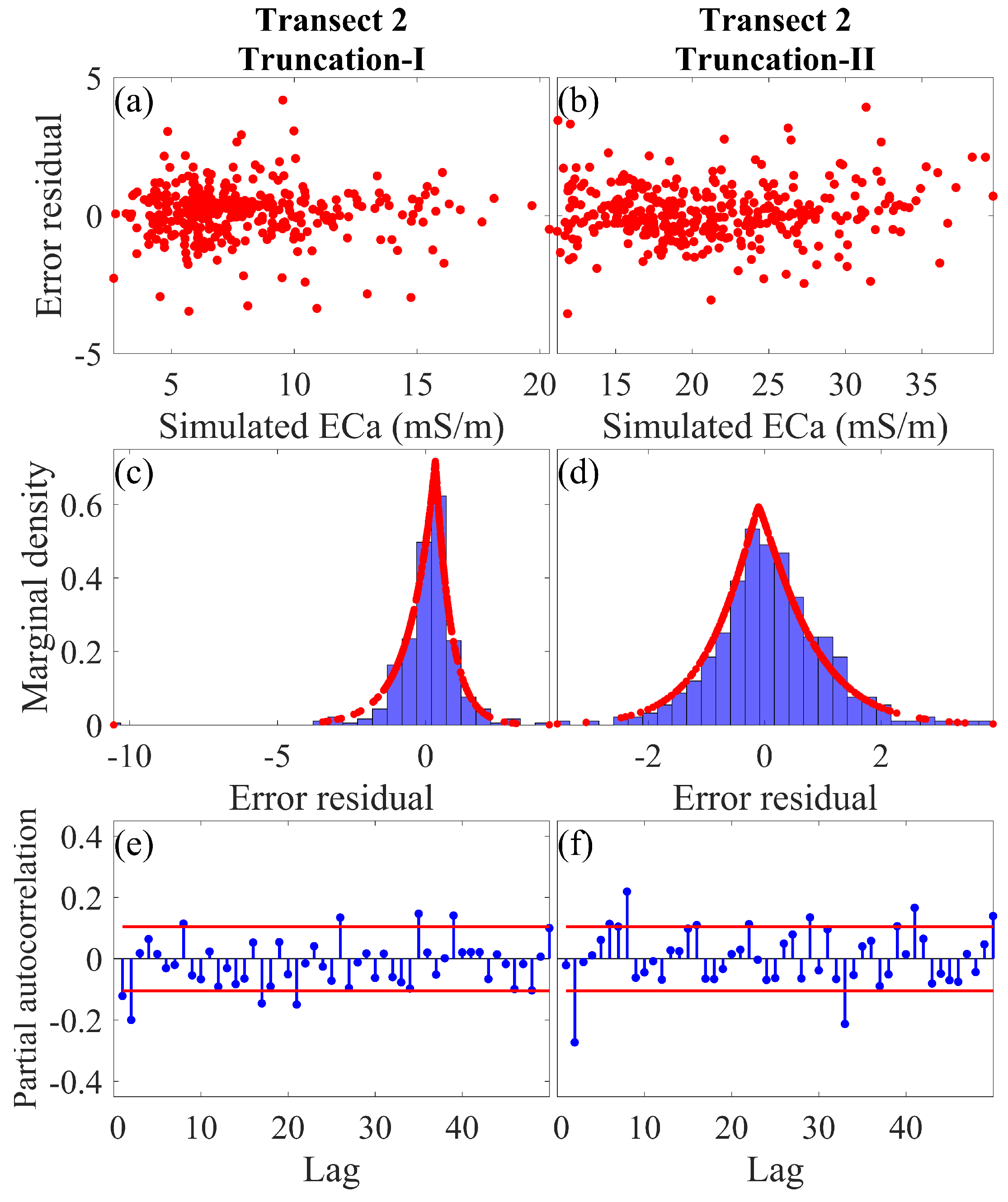
5.4. Transect 2: Inversion Results

We move on to the second transect and present in Figure 9 images of the EC derived from MCMC simulation with the MT-DREAM${}_{\left(\mathrm{ZS}\right)}$ algorithm using the GLF with Truncation-I (top row) and Truncation-II (bottom row). The left and middle columns display the MAP and posterior mean EC field, whereas the right column plots an image of the 95% confidence intervals of the EC values derived from the posterior samples. The results for Transect 2 were in close agreement with those of Transect 1 presented in Figure 5. Indeed, Truncation-I produced a highly-deficient description of the subsurface EC distribution. The MAP and posterior mean images lacked structure and spatial arrangement. The EC values appeared rather constant with depth and did not portray zonal layering. Again, the MAP and posterior mean EC images derived from Truncation-II were in excellent agreement with their counterpart from the ERT survey. The 95% confidence intervals of the posterior EC images were rather tight close to the soil surface and increased downward to the bottom of the measured EMI domain. Figure 10 displays histograms of the RMSE values of the posterior EC images for Truncation-I (light gray) and Truncation-II (dark gray) sampled by the MT-DREAM${}_{\left(\mathrm{ZS}\right)}$ algorithm. The RMSE values derived from Truncation-I (between 13 and 16 mS/m) were substantially larger than most of their counterparts of around 1 mS/m for Truncation-II. This highlights a problem with the choice of the upper and lower bounds of the uniform prior distribution of the DCT coefficients.

Next, we plot in Figure 11 histograms of the marginal posterior distribution of the nuisance variables, $s_0$, $s_1$, $\beta$, $\xi$, and ${\varphi }_1$ of the GLF for Truncation-I (left column) and Truncation-II (right column). The blue and black asterisks in each graph separately indicate the MAP and posterior mean solution of each GLF variable. The results were very similar to those of Transect 1 presented in Figure 7. Indeed, we again observe a close agreement between the MAP and posterior mean values of the nuisance variables. This holds for both truncation methods. Furthermore, most histograms were well described with a normal distribution with the exception of the marginal distribution of $s_0$ and $\beta$ for Truncation-I. Furthermore, the near-zero values of the slope, $s_1$, of the measurement error model suggested that the ECa observations exhibited a constant measurement error standard deviation on the order of 0.1 mS/m, as determined by the posterior values of the intercept, $s_0$ (top panel). The kurtosis, $\beta$, increased from values of 0.2–0.4 for Transect 1 to values of about 0.95 (Truncation-I) and 0.8 (Truncation-II) for Transect 2, respectively. The skewness, $\xi$, on the other hand, took on values of about 0.8 and 1.05 for Truncations-I and -II, respectively, which were remarkably similar to their values of approximately 0.8 and 1.0 for Transect 1. This finding corroborates our earlier findings for Transect 1 that the ECa residuals did not exhibit much skew. Yet, for Transect 2, the ECa residuals were much better described with a Laplacian or double-exponential distribution rather than a Gaussian distribution. The marginal distribution of ${\varphi }_1$ for Truncation-I confirmed the presence of strong serial correlation among the ECa residuals. The autocorrelation reduced to values of ${\varphi }_1$ of about 0.55 for Truncation-II. This finding is in agreement with our results for Transect 1. The poor performance of Truncation-I was symptomatic of the use of inadequate lower and upper bounds for DCT coefficients. Yet, it is not particularly easy to determine suitable ranges of the DCT coefficients without the use of training data images (as done by Truncation-II). In any case, the scaling methodology of Linde and Vrugt [22] may need to be refined for EMI data inversion.

We conclude this paper with a diagnostic check of the ECa residuals of the MAP solution (see Figure 12). We display separately the results for Truncation-I (left column) and Truncation-II (right column). The results of this analysis again confirm our earlier conclusions. The residuals of Truncation-I (Figure 12a) and Truncation-II (Figure 12b) exhibited a constant variance and meander around zero. The magnitude of the ECa residuals appeared rather constant and largely independent of the simulated ECa value. Altogether, the EMI measurement error appeared mostly homoscedastic, a finding supported by the near-zero sampled values of the slope, $s_0$, of the measurement error model (see Figure 11a,b). The histograms of the ECa residuals for Truncations-I and -II in the middle row matched their supposed double-exponential distribution (red line), and the partial autocorrelation functions (bottom row) demonstrated a negligible serial correlation among the first-order decorrelated ECa residuals, $\mathsf{\epsilon }(\mathsf{\theta },{\mathbf{\Phi }}_p)$. Altogether, we conclude that the probabilistic properties of the ECa residuals satisfy their underlying assumptions of the GLF. This inspires confidence in the sampled values of the DCT coefficients. Nevertheless, the values of ${\varphi }_1$ close to unity confirmed that Truncation-I was deficient. The culprit was the prior distribution of the DCT coefficients, which prevented the MT-DREAM${}_{\left(\mathrm{ZS}\right)}$ algorithm from sampling EC fields of similar quality as those derived from Truncation-II.

Before we move on to the conclusion section, we would like to discuss and reiterate a few key points that may be of practical concern and/or importance. In our study, the main features of the EC field were successfully recovered using EM inversion with DCT-based image compression using training data images from the ECa measurements. The work presented here supports the findings by Moghadas [24] that confirmed the robustness of the DCT-based inversion of EMI data using geostatistical prior (Truncation-II) via synthetic scenarios. Moreover, we compared the EC images from the CMD-Explorer sensor measured using a frequency of 10 kHz with ERT models measured at around 1 Hz. As a consequence, we assumed a frequency-independent EC in this frequency range. Since EMI involves a diffusion-type process (due to a low operating frequency), DCT-based inversion of EMI data is not as sensitive to sudden and sharp variations in the measured data. This makes it easier for MCMC simulation to back out the preferred values of the DCT coefficients and simplifies posterior exploration in comparison to EM scattering methods such as ground penetrating radar (GPR) [22]. As our method incorporates all measured ECa data along a transect, it can provide a continuous image of the subsurface EC field with reduced variance. The use of transect data also opens up a wide-arsenal of image compression methods that help cast our Bayesian framework as an over-determined problem (the number of unknown model parameters is far less than the number of measured data points). This is particularly important in the present context as EMI measurements often exhibit limited information about the subsurface apparent electrical conductivity values. Based on our knowledge of the structure of the subsurface at the Chicken Creek watershed, a one-dimensional EM forward model was deemed sufficient to model spatial variations in the EC. This assumption may not be appropriate for subsurface systems with complex multi-dimensional structures. Such (geological) features may demand the use of a more advanced two- or three-dimensional EM models. This will lead to a more accurate subsurface characterization, but at the expense of a significant increase in the computational cost.

6. Conclusions

In this paper, we examined the power and usefulness of two different truncation approaches for model parametrization using discrete cosine transform. We applied a quasi-two-dimensional electromagnetic model to obtain the subsurface electrical conductivity distributions from EMI data measured along two transects in the Chicken Creek catchment (Brandenburg, Germany). Bayesian inference with the MT-DREAM${}_{\left(\mathrm{ZS}\right)}$ algorithm and generalized likelihood function was used to back out the relevant DCT coefficients from measured EMI transect data. Results demonstrated that arbitrary selection of the low-frequency DCT coefficients and the ranges of their prior distribution can prove futile and produce inaccurate subsurface EC fields. Instead, geostatistical simulation of the EMI measured ECa image of each transect using direct sampling provided a robust selection of the low-frequency DCT coefficients and their prior ranges. Model compression via DCT using geostatistical prior modeling thus offers a great promise for accurate subsurface EC imaging from multi-configuration EMI data with low posterior uncertainty. The EC of the subsurface is as function of soil salinity and moisture content. The DCT-based probabilistic EMI inversion framework presented herein may, therefore, hold great promise for characterization of soil water content. Repeated EMI surveys at different field sites must corroborate the potential for soil moisture monitoring. Furthermore, comparison with the other existing inversion techniques warrants further investigation.

References

1. Bradford, J.H.; Clement, W.P.; Barrash, W. Estimating porosity with ground-penetrating radar reflection tomography: A controlled 3-D experiment at the Boise Hydrogeophysical Research Site. Water Resour. Res. 2009, 45, 11. [Google Scholar] [CrossRef]
2. Yao, R.J.; Yang, J.S. Quantitative evaluation of soil salinity and its spatial distribution using electromagnetic induction method. Agric. Water Manag. 2010, 97, 1961–1970. [Google Scholar] [CrossRef]
3. Andre, F.; van Leeuwen, C.; Saussez, S.; Van Durmen, R.; Bogaert, P.; Moghadas, D.; de Resseguier, L.; Delvaux, B.; Vereecken, H.; Lambot, S. High-resolution imaging of a vineyard in south of France using ground-penetrating radar, electromagnetic induction and electrical resistivity tomography. J. Appl. Geophys. 2012, 78, 113–122. [Google Scholar] [CrossRef]
4. Dafflon, B.; Hubbard, S.; Ulrich, C.; Peterson, J.E. Electrical Conductivity Imaging of Active Layer and Permafrost in an Arctic Ecosystem, through Advanced Inversion of Electromagnetic Induction Data. Vadose Zone J. 2013, 12. [Google Scholar] [CrossRef]
5. Von Hebel, C.; Rudolph, S.; Mester, A.; Huisman, J.A.; Kumbhar, P.; Vereecken, H.; van der Kruk, J. Three-dimensional imaging of subsurface structural patterns using quantitative large-scale multiconfiguration electromagnetic induction data. Water Resour. Res. 2014, 50, 2732–2748. [Google Scholar] [CrossRef] [Green Version]
6. Jadoon, K.Z.; Weihermuller, L.; McCabe, M.F.; Moghadas, D.; Vereecken, H.; Lambot, S. Temporal Monitoring of the Soil Freeze-Thaw Cycles over a Snow-Covered Surface by Using Air-Launched Ground-Penetrating Radar. Remote. Sens. 2015, 7, 12041–12056. [Google Scholar] [CrossRef] [Green Version]
7. Moghadas, D.; Jadoon, K.Z.; McCabe, M.F. Spatiotemporal monitoring of soil water content profiles in an irrigated field using probabilistic inversion of time-lapse EMI data. Adv. Water Resour. 2017, 110, 238–248. [Google Scholar] [CrossRef] [Green Version]
8. Robinson, D.A.; Lebron, I.; Kocar, B.; Phan, K.; Sampson, M.; Crook, N.; Fendorf, S. Time-lapse geophysical imaging of soil moisture dynamics in tropical deltaic soils: An aid to interpreting hydrological and geochemical processes. Water Resour. Res. 2009, 45. [Google Scholar] [CrossRef]
9. Triantafilis, J.; Santos, F.A.M. Resolving the spatial distribution of the true electrical conductivity with depth using EM38 and EM31 signal data and a laterally constrained inversion model. Aust. J. Soil Res. 2010, 48, 434–446. [Google Scholar] [CrossRef]
10. Moghadas, D.; Andre, F.; Bradford, J.H.; van der Kruk, J.; Vereecken, H.; Lambot, S. Electromagnetic induction antenna modelling using a linear system of complex antenna transfer functions. Near Surf. Geophys. 2012, 10, 237–247. [Google Scholar] [CrossRef]
11. Huang, J.; Taghizadeh-Mehrjardi, R.; Minasny, B.; Triantafilis, J. Modeling Soil Salinity along a Hillslope in Iran by Inversion of EM38 Data. Soil Sci. Soc. Am. J. 2015, 79, 1142–1153. [Google Scholar] [CrossRef]
12. Huang, J.; Scudiero, E.; Clary, W.; Corwin, D.L.; Triantafilis, J. Time-lapse monitoring of soil water content using electromagnetic conductivity imaging. Soil Use Manag. 2016, 33, 191–204. [Google Scholar] [CrossRef]
13. Mester, A.; van der Kruk, J.; Zimmermann, E.; Vereecken, H. Quantitative Two-Layer Conductivity Inversion of Multi-Configuration Electromagnetic Induction Measurements. Vadose Zone J. 2011, 10, 1319–1330. [Google Scholar] [CrossRef]
14. Robinet, J.; von Hebel, C.; Govers, G.; van der Kruk, J.; Minella, J.P.G.; Schlesner, A.; Ameijeiras-Marino, Y.; Vanderborght, J. Spatial variability of soil water content and soil electrical conductivity across scales derived from Electromagnetic Induction and Time Domain Reflectometry. Geoderma 2018, 314, 160–174. [Google Scholar] [CrossRef]
15. Jadoon, K.Z.; Moghadas, D.; Jadoon, A.; Missimer, T.M.; Al-Mashharawi, S.K.; McCabe, M.F. Estimation of soil salinity in a drip irrigation system by using joint inversion of multicoil electromagnetic induction measurements. Water Resour. Res. 2015, 51, 3490–3504. [Google Scholar] [CrossRef] [Green Version]
16. Triantafilis, J.; Monteiro Santos, F.A. Electromagnetic conductivity imaging (EMCI) of soil using a DUALEM-421 and inversion modelling software (EM4Soil). Geoderma 2013, 211–212, 28–38. [Google Scholar] [CrossRef]
17. Christiansen, A.V.; Pedersen, J.B.; Auken, E.; Soe, N.E.; Holst, M.K.; Kristiansen, S.M. Improved Geoarchaeological Mapping with Electromagnetic Induction Instruments from Dedicated Processing and Inversion. Remote. Sens. 2016, 8, 1022. [Google Scholar] [CrossRef]
18. Auken, E.; Christiansen, A.V.; Kirkegaard, C.; Fiandaca, G.; Schamper, C.; Behroozmand, A.A.; Binley, A.; Nielsen, E.; Efferso, F.; Christensen, N.B.; et al. An overview of a highly versatile forward and stable inverse algorithm for airborne, ground-based and borehole electromagnetic and electric data. Explor. Geophys. 2015, 46, 223–235. [Google Scholar] [CrossRef] [Green Version]
19. Minsley, B.J. A trans-dimensional Bayesian Markov chain Monte Carlo algorithm for model assessment using frequency-domain electromagnetic data. Geophys. J. Int. 2011, 187, 252–272. [Google Scholar] [CrossRef] [Green Version]
20. Jadoon, K.Z.; Altaf, M.U.; McCabe, M.F.; Hoteit, I.; Muhammad, N.; Moghadas, D.; Weihermuller, L. Inferring soil salinity in a drip irrigation system from multi-configuration EMI measurements using adaptive Markov chain Monte Carlo. Hydrol. Earth Syst. Sci. 2017, 21, 5375–5383. [Google Scholar] [CrossRef] [Green Version]
21. Vrugt, J.A.; Ter Braak, C.J.F.; Diks, C.G.H.; Robinson, B.A.; Hyman, J.M.; Higdon, D. Accelerating Markov chain Monte Carlo simulation by differential evolution with self-adaptive randomized subspace sampling. Int. J. Nonlinear Sci. Numer. Simul. 2009, 10, 273–290. [Google Scholar] [CrossRef]
22. Linde, N.; Vrugt, J.A. Distributed Soil Moisture from Crosshole Ground-Penetrating Radar Travel Times using Stochastic Inversion. Vadose Zone J. 2013, 12, 16. [Google Scholar] [CrossRef]
23. Qin, H.; Xie, X.Y.; Vrugt, J.A.; Zeng, K.; Hong, G. Underground structure defect detection and reconstruction using crosshole GPR and Bayesian waveform inversion. Autom. Constr. 2016, 68, 156–169. [Google Scholar] [CrossRef] [Green Version]
24. Moghadas, D. Probabilistic Inversion of Multiconfiguration Electromagnetic Induction Data Using Dimensionality Reduction Technique: A Numerical Study. Vadose Zone J. 2019, 18. [Google Scholar] [CrossRef]
25. Lochbuhler, T.; Vrugt, J.A.; Sadegh, M.; Linde, N. Summary statistics from training images as prior information in probabilistic inversion. Geophys. J. Int. 2015, 201, 157–171. [Google Scholar] [CrossRef] [Green Version]
26. Ahmed, N.; Natarajan, T.; Rao, K.R. Discrete cosine transform. IEEE Trans. Comput. 1974, C 23, 90–93. [Google Scholar] [CrossRef]
27. Gerwin, W.; Schaaf, W.; Biemelt, D.; Fischer, A.; Winter, S.; Huttl, R.F. The artificial catchment “Chicken Creek” (Lusatia, Germany)-A landscape laboratory for interdisciplinary studies of initial ecosystem development. Ecol. Eng. 2009, 35, 1786–1796. [Google Scholar] [CrossRef]
28. Schaaf, W.; Pohle, I.; Maurer, T.; Gerwin, W.; Hinz, C.; Badorreck, A. Water Balance Dynamics during Ten Years of Ecological Development at Chicken Creek Catchment. Vadose Zone J. 2017, 16. [Google Scholar] [CrossRef]
29. Loke, M.H.; Acworth, I.; Dahlin, T. A comparison of smooth and blocky inversion methods in 2D electrical imaging surveys. Explor. Geophys. 2003, 34, 182–187. [Google Scholar] [CrossRef]
30. Wait, J.R. Mutual coupling of loops lying on the ground. Geophysics 1954, 19, 290–296. [Google Scholar] [CrossRef]
31. Ward, S.H.; Hohmann, G.W. Electromagnetic theory for geophysical application. In Electromagnetic Methods in Applied Geophysics; Investigations in Geophysics Series; Nabighian, M.N., Ed.; Society of Exploration Geophysicists: Tulsa, OK, USA, 1987; Volume 1, pp. 131–312. ISBN 978-1-56080-263-1. [Google Scholar]
32. Van der Kruk, J.; Meekes, J.A.C.; van den Berg, P.M.; Fokkema, J.T. An apparent-resistivity concept for low-frequency electromagnetic sounding techniques. Geophys. Prospect. 2000, 48, 1033–1052. [Google Scholar] [CrossRef]
33. Jafarpour, B.; Goyal, V.K.; McLaughlin, D.B.; Freeman, W.T. Transform-domain sparsity regularization for inverse problems in geosciences. Geophysics 2009, 74, R69–R83. [Google Scholar] [CrossRef]
34. Mariethoz, G.; Renard, P.; Straubhaar, J. The Direct Sampling method to perform multiple-point geostatistical simulations. Water Resour. Res. 2010, 46, 14. [Google Scholar] [CrossRef]
35. Meerschman, E.; Pirot, G.; Mariethoz, G.; Straubhaar, J.; Van Meirvenne, M.; Renard, P. A practical guide to performing multiple-point statistical simulations with the Direct Sampling algorithm. Comput. Geosci. 2013, 52, 307–324. [Google Scholar] [CrossRef]
36. Volpi, E.; Schoups, G.; Firmani, G.; Vrugt, J.A. Sworn testimony of the model evidence: Gaussian Mixture Importance (GAME) sampling. Water Resour. Res. 2017, 53, 6133–6158. [Google Scholar] [CrossRef] [Green Version]
37. Schoups, G.; Vrugt, J.A. A formal likelihood function for parameter and predictive inference of hydrologic models with correlated, heteroscedastic, and non-Gaussian errors. Water Resour. Res. 2010, 46, 17. [Google Scholar] [CrossRef]
38. Vrugt, J.A.; Massoud, E.M. Uncertainty quantification of complex system models: Bayesian Analysis. In Handbook of Hydrometeorological Ensemble Forecasting; Duan, Q., Pappenberger, F., Thielen, J., Wood, A., Cloke, H.L., Schaake, J.C., Eds.; Springer: Berlin/Heidelberg, Germany, 2018. [Google Scholar]
39. Laloy, E.; Vrugt, J.A. High-dimensional posterior exploration of hydrologic models using multiple-try DREAM((ZS)) and high-performance computing. Water Resour. Res. 2012, 48. [Google Scholar] [CrossRef]
40. Laloy, E.; Rogiers, B.; Vrugt, J.A.; Mallants, D.; Jacques, D. Efficient posterior exploration of a high-dimensional groundwater model from two- stage Markov chain Monte Carlo simulation and polynomial chaos expansion. Water Resour. Res. 2013, 49, 2664–2682. [Google Scholar] [CrossRef]
41. Rosas-Carbajal, M.; Linde, N.; Kalscheuer, T.; Vrugt, J.A. Two-dimensional probabilistic inversion of plane-wave electromagnetic data: Methodology, model constraints and joint inversion with electrical resistivity data. Geophys. J. Int. 2014, 196, 1508–1524. [Google Scholar] [CrossRef]
42. Gelman, A.; Rubin, D.B. Inference from Iterative Simulation Using Multiple Sequences. Statist. Sci. 1992, 7, 457–472. [Google Scholar] [CrossRef]
43. Vrugt, J.A. Markov chain Monte Carlo simulation using the DREAM software package: Theory, concepts, and MATLAB implementation. Environ. Model. Softw. 2016, 75, 273–316. [Google Scholar] [CrossRef] [Green Version]
44. Box, G.; Tiao, G. Bayesian Inference in Statistical Analysis; John Wiley: New York, NY, USA, 1992; p. 588. [Google Scholar]
45. Fernandez, C.; Steel, M.F.J. On Bayesian modeling of fat tails and skewness. J. Am. Stat. Assoc. 1998, 93, 359–371. [Google Scholar] [CrossRef]
Figure 1. The Chicken Creek catchment located in Lusatia, Germany: (a) areal overview of the main characteristics of the catchment (taken from Schaaf et al. [28]) and (b) bird’s eye view of the two measurement transects (red lines) and direction of the surveys (arrows).
Remotesensing 11 01549 g001
Figure 2. Different truncation approaches for model parametrization: (a) Truncation-I: a structured grid with low-frequency coefficients (colored cells) of matrix G that is used to characterize the electrical conductivity (EC) field in our DCT compression framework. The regular grid is composed of n = 12 × m = 60 cells and characterized by the d = 45 frequencies of the gray colored cells. The 45 low-frequency components and their prior distribution are arbitrarily selected without using geostatistical simulations. (b) Truncation-II: schematic progress of the model parametrization using multiple-point statistical (MPS) simulations. The apparent electrical conductivity (ECa) pseudosection derived from EMI data is considered as a training image (TI) for MPS simulations. The TI realizations are transformed to the frequency domain using DCT. Afterwards, dominant DCT coefficients and their upper and lower bounds are determined from MPS realizations considering a regular grid composed of n = 12 × m = 60 cells.
Remotesensing 11 01549 g002
Figure 3. Inversely-estimated electrical resistivity tomography (ERT) models along with the ECa images: the top panel presents images of the EC of Transects 1 (left) and 2 (right) surveyed by ERT. These images were derived from inversion of the measured ERT resistivity data using the RES2DINV program. The bottom panel displays ECa pseudosections of both transects derived from the EMI data. (a) Transect 1-ERT; (b) Transect 2-ERT; (c) Transect 1-EMI; (d) Transect 2-EMI.
Remotesensing 11 01549 g003
Figure 4. Application of geostatistical simulation to the ECa training data images of Transects 1 (left column) and 2 (right column). The top panel (a,b) presents a sample set of five realizations derived from direct sampling with the DeeSse software; the middle panel (c,d) displays graphically with a gray color the dominant DCT coefficients from the 1000 different DeeSse realizations; the bottom panel (e,f) summarizes the selection of the low frequency DCT coefficients, which were used for image compression in Truncation-II.
Remotesensing 11 01549 g004
Figure 5. Transect 1: MAP, MEAN, and 95% confidence intervals of the subsurface EC field derived from MCMC simulation with the MT-DREAM ( ZS ) algorithm using the generalized likelihood function (GLF) with (ac) Truncation-I and (df) Truncation-II, respectively.
Remotesensing 11 01549 g005
Figure 6. Transect 1: Histograms of the posterior RMSE values sampled by the MT-DREAM ( ZS ) algorithm using Truncation-I (light gray) and Truncation-II (dark gray).
Remotesensing 11 01549 g006
Figure 7. Transect 1: Histograms of the marginal posterior distributions of the nuisance variables of the GLF for Truncation-I (left column) and Truncation-II (right column): (a,b) s 0 ; (c,d) s 1 ; (e,f) β ; (g,h) ξ ; and (i,j) ϕ 1 . The blue and black asterisks in each graph signify the MAP and posterior MEAN solution.
Remotesensing 11 01549 g007
Figure 8. Transect 1: Diagnostic checks of the ECa residuals of the MAP solution sampled with the MT-DREAM ( ZS ) algorithm using the GLF with Truncation I (left column) and Truncation II (right column). (a,b) Two-dimensional scatter plot of the simulated ECa values and the ECa residuals, (c,d) Assumed (solid line) and actual distribution (histogram) of the ECa residuals and (e,f) partial autocorrelation function of the ECa residuals (= autocorrelation function of first-order decorrelated residuals, ε ( θ , Φ p ) ). The solid red lines display the 95% confidence intervals of white noise.
Remotesensing 11 01549 g008
Figure 9. Transect 2: MAP, MEAN, and 95% confidence intervals of the subsurface EC field derived from MCMC simulation with the MT-DREAM ( ZS ) algorithm using the GLF with (ac) Truncation-I and (df) Truncation-II, respectively.
Remotesensing 11 01549 g009
Figure 10. Transect 2: Histograms of the posterior RMSE values sampled by the MT-DREAM ( ZS ) algorithm using Truncation-I and Truncation-II.
Remotesensing 11 01549 g010
Figure 11. Transect 2: Histograms of the marginal posterior distributions of the nuisance variables of the GLF for Truncation-I (left column) and Truncation-II (right column): (a,b) s 0 ; (c,d) s 1 ; (e,f) β ; (g,h) ξ ; and (i,j) ϕ 1 . The blue and black asterisks in each graph signify the MAP and posterior MEAN solution.
Remotesensing 11 01549 g011
Figure 12. Transect 2: Diagnostic checks of the ECa residuals of the MAP solution sampled with the MT-DREAM ( ZS ) algorithm using the GLF with Truncation-I (left column) and Truncation-II (right column). (a,b) Two-dimensional scatter plot of the simulated ECa values and the ECa residuals, (c,d) supposed (red line) and actual distribution (histogram) of the ECa residuals, and (e,f) autocorrelation function of the first-order decorrelated residuals, ε ( θ , Φ p ) . The solid red lines display the 95% confidence intervals of white noise.
Remotesensing 11 01549 g012