Study on Mechanism of Visual Comfort Perception in Urban 3D Landscape

Abstract

Landscape visual evaluation is a key method for assessing the value of visual landscape resources. This study aims to enhance the visual environment and sensory quality of urban landscapes by establishing standards for the visual comfort of urban natural landscapes. Using line-of-sight and multi-factor analysis algorithms, the method assesses spatial visibility and visual exposure of building clusters in the core urban areas of Harbin, identifying areas and viewpoints with high visual potential. Focusing on the viewpoints of landmark 3D models and the surrounding landscape’s visual environment, the study uses the city’s sky, greenery, and water features as key visual elements for evaluating the comfort of urban natural landscapes. By integrating GIS data, big data street-view photos, and image semantic recognition, spatial analysis algorithms extract both objective and subjective visual values at observation points, followed by mathematical modeling and quantitative analysis. The study explores the coupling relationship between objective physical visual values and subjective perceived visibility. The results show that 3D visual analysis effectively reveals the relationship between landmark buildings and surrounding landscapes, providing scientific support for urban planning and contributing to the development of a more distinctive and attractive urban space.

1. Introduction

With the acceleration of urbanization, the current two-dimensional natural landscape supply can no longer meet the growing demand for urban natural landscape perception and experience. The value of the three-dimensionality of urban natural landscape perception is becoming increasingly recognized. The most intuitive measure of the three-dimensional urban natural landscape visual experience is the degree of visual perception and comfort people have towards urban natural landscapes. Therefore, a more reasonable approach is to treat it as a three-dimensional spatial system [1]. This paper comprehensively reveals the composition, layout, and visual characteristics of the landscape from a three-dimensional perspective, providing a more accurate reflection of the spatial structure of the city. Vision is the primary way for humans to acquire information, and urban visual landscapes are one of the key means by which people interpret [2,3], understand, and enjoy cities. In the documentation and analysis of human perception of the environment, the concept of the “natural city” is considered the most complex. In a “natural city”, the interface and interactions between architectural components (such as overall planning, foundational structures, buildings, or street spaces) and natural elements (such as geographical location, terrain, water bodies, and vegetation) are highly complex, providing environmental planners and designers with a rich, diverse, and multi-layered field of study. The ecological value of urban natural resources has long been a focus of attention, but the value of visual landscapes is often overlooked. Although landscape perception is the result of a multi-sensory experience, landscape visibility is fundamental to this perceptual experience. The visual relationship between the observer’s position and the target landscape plays a critical role in constructing the significance of the landscape for the observer [4].

Since the 21st century, the exponentially growing process of urbanization worldwide, along with the continuous vertical expansion and outward sprawl of urban spaces, has driven the need for urban three-dimensional spatial visual studies that align with the demands of the new era. To study the complexities of urban visual spaces, the Centre for Advanced Spatial Analysis (CASA) at University College London (UCL) developed the urban spatial analysis software Depthmap, which enables the analysis of isovist (visible space) [5]. In 2003, Marcos Llobera, an archeologist at the University of Washington, redefined the term “Visualscape” within the context of Geographic Information System Science and offered a more rigorous description of the quantitative indicators for spatial visualization [6]. And international research on visual landscape resources has expanded into various fields, including geography [7], forestry [8], tourism [9], and psychology [10]. Numerous experts have conducted studies quantitatively describing the impact of visual landscapes and establishing landscape visual indicator systems from different perspectives. Scholars abroad, such as Lothian [11], have categorized landscape aesthetics into objective and subjective branches using philosophy and aesthetic theory and developed a scenic aesthetic model integrating both objective and subjective principles, providing theoretical support for the evolutionary aesthetics of landscapes. Ayad et al. [12] used RS (Remote Sensing) and GIS (Geographic Information System) technology to model and evaluate the visual changes along Egypt’s arid northwest coast over forty years.

Nevertheless, studies both domestically and internationally highlight a notable gap in quantitative analyses of urban visual spaces, particularly on a large scale, and emphasize the limited consideration of urban spaces from a holistic viewpoint. The emergence of urban design signifies a shift in urban planning approaches, evolving from traditional two-dimensional frameworks to three-dimensional and even four-dimensional models that incorporate temporal changes. Urban design seeks to integrate the roles of architecture, planning, and landscape within urban spaces, fostering coordination among these elements from a three-dimensional perspective. At present, most urban visual quantitative landscape analyses are conducted primarily on a two-dimensional plane. However, with the increasing complexity of urban environments, two-dimensional analysis has become insufficient to manage the intricate urban spaces effectively [13,14,15]. In the absence of spatial information, the results of two-dimensional analysis tend to be rough, which in turn can lead to insufficiently effective control strategies in subsequent planning and management. With the continuous advancement of digital technology, urban space management is gradually shifting toward a multi-information integrated management model based on three-dimensional digital cities [16,17,18,19].The structure of this paper is as follows: Section 2 introduces the research methods and data sources, detailing the integration of 3D city modeling, line-of-sight analysis, and multi-factor analysis. Section 3 presents the background of the study area and data collection process, discussing the relevance of Harbin as a case study. Section 4 showcases the results of the visibility analysis based on the proposed methods and discusses the findings. Finally, Section 5 summarizes the main conclusions of the study and offers suggestions for future research on urban landscape visibility analysis.

2. Area and Data Sources

2.1. Study Area Overview

Harbin is located in Northeast China and is the capital city of Heilongjiang Province. The study area map is shown in Figure 1, situated within the Songhua River Basin. The boundary coordinates of Harbin City are longitude 125°41′30″ to 130°13′40″ and latitude 44°03′30″ to 46°40′20″. The total land area is 53,076.4 square kilometers, of which the urban area covers 10,198 square kilometers. As one of the central cities in Northeast China, Harbin is notable for its historical, cultural, and natural landscapes. Additionally, Harbin possesses abundant natural and cultural resources, including several large parks, wetlands, and other natural landscapes within the city. Cultural landmarks such as Central Street, the Flood Control Monument, and Saint Sophia Cathedral provide a wealth of subjects for urban visual landscape studies.

2.2. Data Sources

This study utilizes medium-resolution remote sensing imagery, primarily obtained from the Landsat 8 satellite, which has a spatial resolution of 30 m for multispectral bands and 15 m for panchromatic bands. The Landsat 8 images referenced in the data section were primarily used to extract spatial distribution information of Harbin’s topography, landforms, and major natural landscape features such as rivers and vegetation. The images were acquired during the period of 2018–2020. Multispectral Bands (Bands 2, 3, 4, 5): These bands were used for urban zoning analysis, land cover classification, and extraction of key geographic features like urban areas, buildings, and vegetation. Panchromatic Band (Band 8): This high-resolution band was used in combination with other data sources to improve the accuracy of the DEM (Digital Elevation Model) for elevation analysis. Other Bands (Bands 4, 5, 6): These were used in traffic accessibility and green space analysis, with Bands 4 (Red), 5 (Near-Infrared), and 6 (Shortwave Infrared) helping assess road networks, traffic density, and vegetation classification. These images and bands provide a comprehensive foundation for the visual and spatial analysis conducted in this study. These images were used to extract spatial distribution information on Harbin’s topography, landforms, and major natural landscape elements, such as rivers and vegetation. Spatial data on urban buildings, street networks, and green space distribution were also sourced, along with open online geographic information platforms like OpenStreetMap. For 3D visual analysis, this study employs 3D building model data of Harbin’s central urban area. These datasets provide a robust foundation for the 3D visual landscape analysis of Harbin, ensuring the scientific validity and practical applicability of the research results.

3. Methods

As shown in Technical Roadmap Figure 2, the visual characteristics of urban landscapes are systematically quantified and evaluated through digital model construction and visibility analysis. Using 3D models and multi-factor analysis, spatial relationships among urban topography, buildings, and key viewpoints are established. Visibility between viewpoints and target objects is analyzed based on factors such as transportation accessibility, skyline, and landscape ecology. Finally, the results are visualized to display visibility and landscape value across different areas, providing scientific support for urban planning.

3.1. Principles of Urban Landscape Visual Analysis and Evaluation

Basic Visual Analysis Units

Basic visual analysis units are fundamental elements used to evaluate and analyze visual characteristics within a landscape or urban environment. These units typically include: Viewshed (Visibility Area), Spatial Viewpoints, and Visual Cone (Field of View) [20]. The three proposed basic visual analysis units share a consistent operational model, all based on assessing visibility by determining whether the line of sight between the viewpoint and the target landscape is obstructed. Among these units, the viewshed serves as a two-dimensional analysis (or 2.5D, pseudo-3D) and acts as a preliminary assessment tool to identify visible areas over a large scale. In urban spaces that lack strict design control, public spaces with viewing potential may have been overlooked by existing plans, but viewshed analysis can help researchers identify these potentially overlooked yet valuable scenic areas. Meanwhile, the spatial visibility point set and visual cone analyses are based on 3D spatial models, involving highly data-intensive processes [21]. In urban studies, these models often require computationally intensive datasets containing billions of data points. Before conducting detailed computations, efficient two-dimensional spatial analysis serves as an initial screening process, permitting only the most promising viewpoints to advance to the 3D visual analysis stage. Spatial visibility point sets and visual cones generate a range of quantifiable visual characteristics, enabling this study to both scientifically and intuitively evaluate the visual effects from diverse viewpoints. Quantitative visual indicators are urban spatial metrics derived from these basic visual analysis components, with visibility serving as the most fundamental metric. Visibility refers to whether, and to what extent, a target object is visible from a specific viewpoint, but it does not convey any intrinsic attributes of the physical space. In this context, the concept of the “visual scene” is introduced to more effectively articulate the essential components of quantitative visual landscape metrics.

3.2. Method for Obtaining Spatial Visibility Point Set Analysis Units

3.2.1. Line-of-Sight Algorithm

The basic principle of the line-of-sight (LOS) algorithm is based on the principle of light propagation, where light travels in a straight line [22]. This algorithm calculates visibility between two points or from one point to multiple points. The specific process of line-of-sight analysis begins by generating a ray from the viewpoint to the target point. The algorithm then uses the terrain and existing obstacles (such as vegetation, buildings, and other structures) to determine whether the target point is visible from the viewpoint, as illustrated in Figure 3a,b. In practical scenarios, visibility is influenced by Earth’s curvature and atmospheric refraction. When the distance between the viewpoint and the target point is sufficiently large, the bending effect of light due to curvature and refraction can significantly impact visibility analysis results. Corrections for curvature and atmospheric refraction can be applied by selecting an appropriate coordinate system and using correction formulas. Correction Formula (1) is as follows:

$$Z={\displaystyle \frac{[Z_0+D^2(R-1)]}{d}}$$

(1)

where Z is the corrected elevation considering the atmospheric refraction, Z₀ is the surface elevation at the viewpoint, D is the horizontal distance between the viewpoint and the target point, d is the Earth’s diameter (12,740 km), and R is the refraction coefficient of light (0.13 under standard atmospheric conditions).

3.2.2. Extraction of Visible Sightlines

The spatial visibility point set includes three components: the viewpoint, the control points of visible objects, and the visible space between them [23]. This study primarily focuses on the mutual visibility between the viewpoint and target objects, so only the line-of-sight (visible sightline) between the viewpoint and the target control points is extracted for analysis. By analyzing the unobstructed sightlines between the viewpoint and the target control points, a spatial visibility point set relative to a specific viewpoint can be obtained, representing the control points of target objects visible from that viewpoint. The spatial visibility point set is derived from a 3D model, and if the urban 3D model is sufficiently comprehensive and accurate, the visibility analysis results of the spatial visibility point set will closely match the actual visibility in real-world scenarios.

Figure 3 shows a visibility analysis model of certain areas, where the red region represents the invisible area, and the green region represents the visible area. By analyzing these images, the sightlines (visible sightlines) between the viewpoint and the target control points can be extracted, thereby obtaining a spatial visibility point set relative to a specific viewpoint, which represents the control points of the target objects visible from that viewpoint.

3.3. Visual Quantitative Analysis

3.3.1. Preliminary Selection and Screening of Viewing Points

The control of viewing landscapes is based on a comprehensive analysis of existing viewing resources, first clarifying the importance and value of viewing points and landscapes within the city [20,24,25]. Multiple viewpoints are selected appropriately, and after performing viewshed analysis, building height control results are calculated to manage the core control zone of the view corridor and surrounding coordination zones. This approach aims to protect valuable viewing resources within the city. Given the public and social nature of viewing landscapes, the selection of viewing points should consider not only the terrain conditions of the objects being viewed but also the location of the viewing points, the accessibility of the area, its popularity among residents and tourists, and the quality of the view from each point. Therefore, viewing points should be located at key open space nodes within the city. Viewing points should be open, shared, and situated within accessible urban spaces that can accommodate sufficient numbers of residents and tourists for extended visits. They should provide comfortable environments, allow for easy mobility, and offer clear sightlines to the scenic target while ensuring safety for visitors. The basic selection principles for preliminary viewing point selection are summarized as follows [26,27,28]:

First, Transportation Accessibility: Locations that are easily accessible by public transportation and have convenient parking for vehicles;

Second, Public Gathering Capacity: Open spaces that are easy for the public to access and provide a high level of safety.

There are many factors influencing the selection of viewing points, and it is essential to prioritize key factors by importance, making an effective evaluation system necessary. The Analytic Hierarchy Process (AHP) is a multi-criteria strategy suitable for developing a viewing point evaluation system. This method, first proposed by Saaty, is a hierarchical weight decision-making approach that can be divided into the following steps: 1. establish a judgment matrix; 2. create a single-factor evaluation matrix to assess the importance of each evaluation factor; 3. normalize the analysis results and conduct a consistency check. After obtaining the weight score for each evaluation factor, the evaluation score for each viewing point is calculated in ArcGIS to produce the corresponding analysis results. The detailed steps are as follows:

• Establish the Judgment Matrix: Based on the comparison rules in

  Table 1. Judgment Matrix Scale and Comparison Rules.

  Importance Level Pij	9	7	5	3	1	1/3	1/5	1/7	1/9
  Degree of Importance	Extremely Important	Very Important	Important	Somewhat Important	Not Important	Relatively Unimport-ant	Slightly Importa-nt	Not Important	Very Unimportant

  Note: The importance level Pij indicates the degree of importance of element Pi, with choices available as 8, 6, 4, 2, or 1/2, 1/4, 1/6, 1/8, etc.

  , assess and score the importance of the seven influencing factors. This process ultimately produces the judgment matrix for the evaluation factors affecting the viewpoints;
• Single-Factor Weight Calculation: After establishing the judgment matrix for single-factor evaluation, each result in the matrix needs to be normalized according to the following formula to obtain the final weight.

$$\overline{Pij}={\displaystyle \frac{P\mathrm{ij}}{{\displaystyle \sum _{\mathrm{k}=1}^{\mathrm{n}}\overline{Pij}}}}$$

(2)

$$\overline{W\mathrm{i}}={\displaystyle \sum _{\mathrm{j}}^{\mathrm{n}}\overline{Pij}(i,j=1,2,3...n)}$$

(3)

$$W\mathrm{i}={\displaystyle \frac{\overline{Wi}}{{\displaystyle {\sum }_{\mathrm{j}=1}^{\mathrm{n}}W\mathrm{j}}}}(i,i=1,2,3...n)$$

(4)

First, substitute the comparison results of each factor, denoted as $\overline{P\mathrm{ij}}$, into Formula (2) to obtain the normalized result $W\mathrm{i}$ and the comparison matrix. Then, sum $\overline{P\mathrm{ij}}$ according to Formula (3) to obtain $\overline{W\mathrm{i}}$. Finally, use Formula (4) to calculate the result.

3.

Consistency Check: Since the weights of the factors above are derived from mutual comparisons and lack a fixed reference standard, it is necessary to conduct a consistency check on the evaluation results to avoid errors. The formula and steps for the consistency check are as follows:

$$CI={\displaystyle \frac{\lambda \max -n}{n-1}}$$

(5)

$$CR={\displaystyle \frac{CI}{RI}}$$

(6)

First, multiply the normalized result of each column by the corresponding factor weight Wi, and then sum the products for each row to obtain the consistency vector. Next, calculate the average of the consistency vector to find the max, and substitute it into Formula (5) to obtain the consistency index CI. Finally, substitute the consistency index CI into Formula (6) to calculate the CR value (where RI is a constant).

3.3.2. Measurement of Visual Exposure

Non-binary visibility considers the distance factor of sightlines, whereas in detailed 3D spatial models, more comprehensive visibility analysis can be performed. Accessibility of Sight Lines (ASL) takes into account not only the distance but also the angle between the sightline and the target plane. ASL provides a more accurate representation of the visibility relationship between the observer point and the target point. Visual exposure (VE) describes the degree of attention a target point receives within the urban visual landscape environment. In areas with high visual exposure, even minor changes are keenly perceived by observers, while changes in areas with low visual exposure tend to be noticed more sluggishly.

The height information for visibility analysis comes from the city’s 3D model, generated using high-resolution LiDAR data and satellite imagery, which includes the heights of buildings and natural terrain. These data are crucial for accurately calculating visibility relationships and ensuring the correct positioning of buildings and landmarks from the observer’s viewpoint. If there are m viewpoints (P1, P2, ..., Pm) from which the target point PT is visible, where m represents the number of viewpoints observing the target point, then the visual exposure of PT is defined as follows in Formula (7):

$$VE={\displaystyle {\sum }_{i=1}^{m}AS{L}_{\mathrm{ij}}}$$

(7)

Visual exposure reveals the degree to which buildings and building groups are observed. A higher value indicates that the area represented by the target point is more easily appreciated in its entirety from the viewpoint, while a lower value suggests that the area represented by the target point has a lower exposure from the viewpoint and cannot fully showcase its overall appearance. The average visual exposure of sightlines measures the average degree of attention received by a visible target building point within an urban cluster. A low average visual exposure indicates that the average projected area of that point from the viewpoint is small, resulting in a lower average degree of attention received. The calculation method for average exposure is shown in Formula (8).

$$V{E}_{\mathrm{avg}}={\displaystyle \frac{1}{\mathrm{m}}}\times VE$$

(8)

4. Results and Analysis

This study applies the line-of-sight-based visual analysis method proposed earlier to a case study of Harbin, focusing on the city’s central urban area as the research region. The analysis considers the Songhua River and its surrounding buildings and natural landscapes as visual objects, integrating them with the city’s spatial structure to explore the intrinsic relationships within Harbin’s visual space. The analysis specifically examines the visibility and visual prominence of these landscapes within the city, the visual connectivity between different landscapes, and how they fit into the city’s overall spatial framework. Based on the results of the visual analysis, this paper provides planning and design recommendations to protect and enhance Harbin’s visual landscapes, helping to preserve and strengthen the city’s unique character.

4.1. Analysis Method for Selecting Viewing Points

Through multi-factor analysis, we identified the key factors affecting building height and assigned them different weights based on their significance. By collecting vector data on terrain, buildings, roads, mountains, and water bodies, a model is established in ArcGIS, which addresses some limitations of visibility analysis methods in large-scale urban design. This approach is suitable for meeting the economic needs of most cities in their development. However, from the perspective of quantitative precision alone, it may lead to the omission of unique landscapes and historical buildings in urban design.

Therefore, combining visibility analysis with multi-factor analysis can address the limitations of using a single method, making urban design more comprehensive. Visibility analysis refers to modeling the areas of important urban nodes within the range of human sight, controlling the height of buildings in urban areas. This method is mainly applicable for the preservation of historical buildings, which helps to highlight the city’s characteristics, but it also has certain drawbacks. Controlling the urban skyline may lead to the phenomenon where buildings are taller on the sides and lower in the center, similar to a canyon effect. Additionally, traditional control methods typically rely on simple empirical estimates. Thus, the integration of visibility analysis and multi-factor analysis serves to complement this deficiency.

The land use data shown in Figure 4 indicate that buildings in Harbin are primarily concentrated in the central urban area. Given this, multiple viewpoints are selected within densely built areas to ensure a clear observation of the overall layout of buildings and their interactions with surrounding natural landscapes, such as green spaces and rivers. This serves as a key criterion for selecting viewpoints. Priority is given to locations with open views, such as main roads and plazas, to facilitate an in-depth analysis of the visual impact of building clusters.

Transportation accessibility directly affects the accessibility of observation points. In urban environments, accessibility is a critical factor for residents and tourists to experience visual landscapes, particularly for urban landmarks and public spaces. Buildings in the city center are densely concentrated and well-connected to the road network, facilitating the observation of building layouts (Figure 5a,b). In areas close to major rivers, the cityscape can be viewed from both sides of the waterway, enabling an analysis of the impact of water bodies on building visibility. The high-rise building clusters offer the advantage of observing the density and layered arrangement of structures from elevated viewpoints. According to POI (Point of Interest) data factors (Figure 5c), the main urban area has the highest density of POI distributions, indicating its dominant role in the city and its strong contribution to the city’s economic development. Green space analysis (Figure 5d) shows that green areas are relatively scarce in the main urban area compared to other regions, primarily due to the high density of buildings, with parks and forested areas being comparatively limited. Landscape ecology represents the interaction between natural elements (such as vegetation and water bodies) and urban spaces. These interactions directly influence visual quality by integrating ecological aesthetics into the visibility framework.

Consequently, this study sets viewpoints near landmark buildings to analyze their prominence and visibility within the city skyline. By selecting these factors, the study enables a comprehensive assessment of the visibility in densely built areas and allows for comparisons with surrounding natural landscapes, providing a basis for urban planning and landscape design.

The selection of viewpoints in visual landscape analysis is influenced by several key factors, including the physical accessibility of the location, the surrounding environment, and the vantage point’s ability to capture significant features of the urban or natural landscape. Accessibility plays a critical role, as viewpoints situated along major roads, public spaces, or elevated areas are easier to reach and offer clearer, unobstructed views. Additionally, the spatial arrangement and density of buildings in the area impact how well landmarks or natural features are visible, with open spaces providing better sightlines compared to densely built-up areas. The presence of significant natural elements, such as rivers or green spaces, also contributes to viewpoint selection, as they enhance the visual appeal and interaction between urban and natural landscapes. The prominence and visual impact of the landmark or focal point itself are also key considerations, with viewpoints that highlight the unique characteristics of the landmark, like its height or architectural style, being prioritized. These factors collectively ensure that the selected viewpoints provide a comprehensive and representative visual experience of the landscape while also facilitating the design and preservation of the urban environment.

Figure 5, based on the land use data in Figure 4, shows that the buildings in Harbin are mainly concentrated in the central urban area, providing a basis for subsequent viewpoint selection. Further analysis, considering four other influencing factors, reveals that the central urban area (indicated by the red circle on the left side of the map) stands out across all indicators, further highlighting its dominant role in the city. Therefore, focusing the selection of landmark buildings and viewpoints in the central urban area not only more effectively reflects the core features of the city’s landscape pattern but also better showcases the overall image and functional distribution of the city. After selecting the appropriate visual factors, we will proceed to statistical analysis to quantify the impact of these factors on the urban landscape.

4.2. Landscape Visual Analysis Based on Multiple Building Clusters

This section provides a detailed explanation of the statistical analysis methods used to evaluate the visibility of urban landscapes. By quantitatively analyzing various visual factors, we can gain a clearer understanding of how these factors influence the visibility of buildings and natural landscapes in the city. These statistical methods were chosen because they allow for the quantification of relationships between different factors, providing data-driven support for urban planners to optimize spatial layouts and enhance the visual experience of the landscape.

First, this study utilized high-resolution LiDAR datasets to accurately capture the elevation and structural details of the buildings, as well as the changes in the surrounding terrain, ensuring vertical accuracy in the models. To further refine the visual features of the buildings, high-resolution satellite imagery was incorporated, providing texture and surface details for the models. Additionally, ground-level photographs and aerial images were processed using photogrammetry techniques to generate detailed 3D texture-mapped models. The overall city model was derived from multiple data sources, which provided the geometric layout of the city and surrounding buildings, ultimately helping to construct an accurate urban environment model. By integrating these data sources and employing advanced 3D modeling and spatial analysis techniques, the models of the Flood Control Monument and Saint Sophia Cathedral were generated. The Flood Control Monument is located at the northern end of Central Street in Daoli District, Harbin, Heilongjiang Province, specifically at the intersection of Stalin Street and Flood Control Alley, near Stalin Park along the Songhua River. Saint Sophia Cathedral is located at 88 Toulong Street, Daoli District, Harbin, Heilongjiang Province.

In the landscape visual analysis of Harbin, the spatial distribution of building clusters has a profound impact on the overall visual experience of the city. The distance between buildings and their relative heights determines the spatial density and sense of openness in the city. Additionally, in Harbin’s visual landscape, the building clusters along both sides of the Songhua River serve as key visual guiding elements. The arrangement and height control of these buildings create visual continuity and also direct citizens’ lines of sight and movement paths within the physical space. Especially at key urban nodes, such as the Flood Control Monument and along Central Street, building clusters are connected through symmetrical layouts and distant structures, shifting the city’s focus from historical landmarks to modern urban landscapes and establishing a unique visual order for Harbin.

In the landscape visual analysis of Harbin, the Flood Control Monument (Figure 6a) and Saint Sophia Cathedral (Figure 6b) are two highly representative landmark buildings. They hold significant positions in the city’s historical and cultural heritage, serving as key nodes for selecting visual focal points. Analyzing viewpoint selection for these two landmarks reveals their roles in the city’s spatial layout and their influence on the overall visual experience. Distant Viewpoints: From the opposite bank of the Songhua River or from the Songhua River Bridge, the height and unique shape of the Flood Control Monument are clearly visible against the expansive water background. These distant viewpoints use the open river and sky as a backdrop to highlight the monument’s commemorative and symbolic qualities. Close-Up Viewpoints: From the plaza where the Flood Control Monument is located and nearby pedestrian areas, the monument appears from below at an upward angle. Here, the interaction between the surrounding buildings and the open plaza creates a strong contrast between the monument’s vertical lines and the horizontal space of the plaza.

Figure 7 shows viewpoints selected from five different directions (F1–F5, S1–S5) arranged around a landmark building in Harbin. The figure presents the front view of the building as seen from both a top-down plan view and an actual photograph, along with two different 3D sectional views (left view and right view) from distinct angles. Based on these statistical results, the next step is to further explore the visual impact of building clusters through spatial layout analysis.

4.3. Exploring the Relationship Between Building Distribution and Visual Impact

This study conducts a visibility analysis of a landmark building in Harbin, examining its relationship with the spatial distribution of surrounding buildings. Five representative viewpoints were selected to perform a skyline visibility analysis, aimed at evaluating the visual impact of the building from different perspectives. Using the skyline analysis method, visibility was quantitatively and qualitatively assessed from five different viewpoints around the landmark. This method evaluates the prominence of the building in the urban landscape by analyzing its height within the line of sight, the degree of obstruction, and its impact on the surrounding scenery.

As shown in Figure 8, Impact of Perspective on Visibility: From closer viewpoints (such as the city center), the landmark building’s height allows it to stand out among surrounding buildings, ensuring high visibility. However, as the viewpoint distance increases, the visibility of the landmark is gradually diminished by variations in surrounding high-rise buildings and terrain. The landmark’s visibility is reduced in areas with taller surrounding buildings, as shown by the skyline analysis. In areas densely populated with tall buildings, the landmark’s skyline prominence is reduced, whereas in areas with lower or open buildings, its visibility is significantly enhanced, becoming a focal point in the visual landscape.

Viewpoint F1, being directly facing the building, offers the highest visibility, allowing observers to intuitively perceive the overall structure and grandeur of the building. Viewpoints F2 and F3 provide oblique side views of the building, maintaining relatively high visibility and effectively showcasing the side profile of the structure. Viewpoints F4 and F5 gradually move away from the building and shift outward, which may result in partial obstruction by surrounding buildings and vegetation, leading to a relative decrease in visibility.

As shown in

Table 2. Flood Control Monument Visibility Analysis.

Visibility Level	Area (m2)	Area Percentage (%)	Viewpoint Distribution	Visibility Rating
1	34.85	24.85	F1	Extremely High Visibility (A Grade)
2	20.41	19.97	F2	High Visibility (B Grade)
3	18.64	18.66	F3	Medium-High Visibility (C Grade)
4	10.69	15.32%	F5	Low Visibility (D Grade)
5	8.42	12.91%	F4	Low Visibility (D Grade)

, viewpoint F1 is rated as “Very High Visibility” (Grade A) and covers the largest area, accounting for 24.85% of the total area. This indicates that F1 provides the best visual experience and is the most ideal position for observing the target building or landmark. In terms of layout, F1 is likely situated in a position that directly faces the building with minimal obstructions, thus achieving the highest visibility level. Viewpoints F2 and F3 are rated as “High Visibility” (Grade B) and “Moderate-High Visibility” (Grade C), with area proportions of 19.97% and 18.66%, respectively. This suggests that, while these viewpoints do not offer as high visibility as F1, they still allow for a relatively good view of the building’s main features, making them suitable as secondary observation points. These viewpoints are likely positioned at the side or a bit further from the building, resulting in slightly reduced visibility. Viewpoints F4 and F5 are rated as “Low Visibility” (Grade D), with area proportions of 15.32% and 12.91%, respectively. These areas have poorer visibility, and observers may experience partial obstruction from surrounding buildings or vegetation, making it difficult to view the target building in its entirety. These viewpoints are often located behind the building, in corners, or in areas blocked by other tall structures.

From

Table 3. Saint Sophia Cathedral Visibility Analysis.

Visibility Level	Area (m2)	Area Percentage (%)	Viewpoint Distribution	Visibility Rating
1	66.42	30.97	S2	Extremely High Visibility (A Grade)
2	42.64	18.70	S1	High Visibility (B Grade)
3	26.73	12.19	S3	Medium-High Visibility (C Grade)
4	21.85	11.69	S4	Medium-High Visibility (C Grade)
5	9.42	11.71	S5	Medium-High Visibility (C Grade)

, it can be seen that viewpoint S2 was rated as Extremely High Visibility (A Grade), making it the most visible viewpoint. From this perspective, observers can achieve the best visual experience, with the building’s appearance and details clearly visible, without significant obstruction.

Viewpoint S1 was rated as High Visibility (B Grade). This viewpoint still allows for a good observation of the building’s main features, although some side aspects may be obstructed, resulting in an overall visual effect slightly inferior to S2.

The other viewpoints (S3, S4, S5) were categorized as Medium-High Visibility (C Grade). These viewpoints have weaker visibility, with portions of the building obscured, preventing observers from fully observing the complete structure of the building.

The experimental results indicate that the visibility of the building is closely related to its coverage area. The table shows that the area within the Extremely High Visibility (A Grade) range is 66.42 m², accounting for 30.97% of the total area. This means that approximately one-third of the area can achieve the best observation effect.

The area of the High Visibility (B Grade) zone is 42.64 m², accounting for 18.70% of the total area. This area has slightly lower visibility than Grade A but still maintains a high level of visibility.

The Medium-High Visibility (C Grade) area is more widely distributed, occupying the remaining portion of the total area. The visibility areas for S3, S4, and S5 are 26.73 m², 21.85 m², and 9.42 m², respectively, with proportions of 12.19%, 11.69%, and 11.71%.

4.4. Calculation Based on Spatial Visual Quantification and Viewpoint Coupling

The calculation of viewpoint coupling based on spatial visual quantification is primarily used to analyze the visual coverage and mutual influence among multiple viewpoints, thereby optimizing the visibility of buildings, urban landscapes, or landmarks. By coupling multiple viewpoints, the overlapping visibility ranges, independence, and contribution values of each viewpoint can be analyzed to achieve more precise urban planning and landscape design.

By calculating the coupling coefficients between various viewpoints, the shared visibility range of multiple viewpoints can be assessed. The coupling coefficient represents the degree of visual contribution and redundancy between viewpoints. The calculation formula is as follows:

$$C_{\mathrm{ij}}={\displaystyle \frac{A_{\mathrm{ij}}}{A_{\mathrm{i}}+A_{\mathrm{j}}-A_{\mathrm{ij}}}}$$

(9)

where A_ij represents the area of overlap between the visibility regions of viewpoint i and viewpoint j, while A_i and A_j represent the visibility areas of viewpoint iii and viewpoint j, respectively. By calculating the degree of overlap between the visibility domains of the viewpoints, the independence and complementarity of each viewpoint can be assessed. If two viewpoints have a high degree of overlap in their visibility domains, it indicates that their contributions are redundant. Conversely, if there is minimal overlap, it suggests that the two viewpoints have good complementarity and are suitable for coupling design.

From the viewpoints selected in Figure 9’s aerial perspective images, Figure 9a captures an expansive perspective of the Songhua River Basin, showcasing the surrounding environment of the Flood Control Memorial Tower. The scene includes a significant portion of water bodies, vegetation, and urban buildings, illustrating the prominent position of the Flood Control Memorial Tower as one of the core landscapes in the city, and its integration with both natural and urban elements. This perspective offers a direct view of the riverside landscape layout, as well as the spatial relationship between the tower, the river, and the city.

Figure 9b is taken from a more elevated angle, primarily displaying a comprehensive view of the Flood Control Memorial Tower and its surrounding square layout. This perspective places the memorial tower at the center of the frame, with the greenery and square space clearly visible, reflecting the openness of this landmark and its function as an urban public space.

Figure 9c presents a frontal approach towards Saint Sophia Cathedral, highlighting its unique Byzantine architectural features. The surrounding buildings and plaza are included, creating an overall atmosphere rich in history and urban vitality. This perspective also emphasizes the cathedral’s central role as a significant landmark within the cultural landscape of the city.

Figure 9d shows a side view of Saint Sophia Cathedral, where its onion-shaped dome contrasts with the surrounding modern buildings, highlighting the connection between historic and modern architecture. This perspective also underscores the cathedral’s prominent position in the city.

As shown in Figure 10, these two sets of images, respectively, display the multi-viewpoint 3D model visibility analysis of the Flood Control Memorial Tower (F1–F5) and Saint Sophia Cathedral (S1–S5). Each set of images is captured from different perspectives, demonstrating the spatial relationship between the landmark and its surrounding environment.

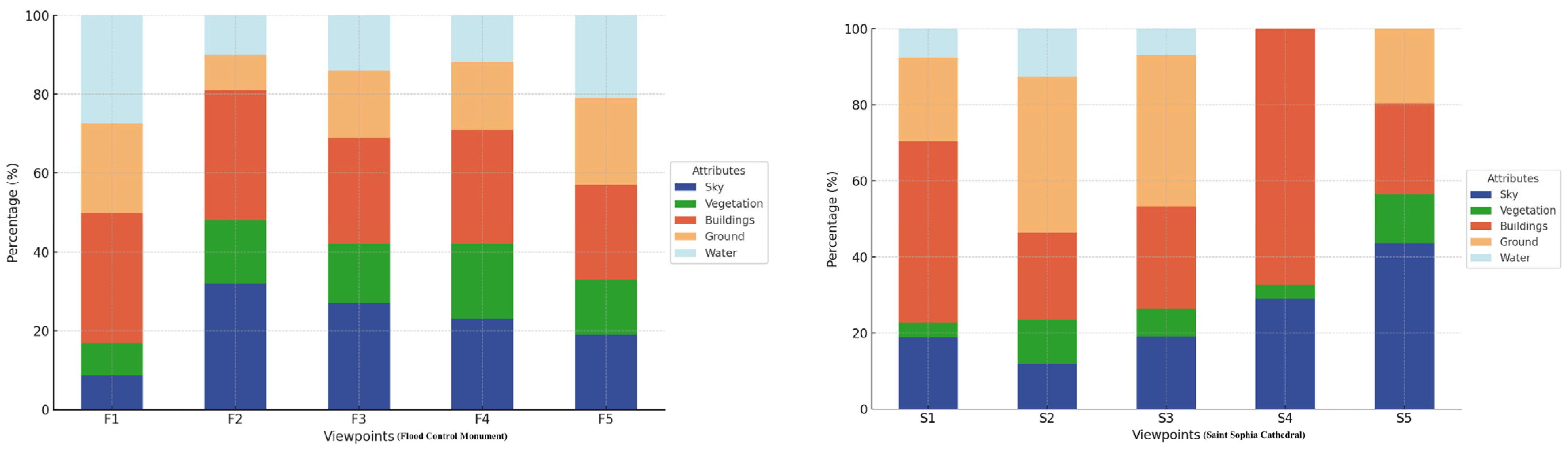
As shown in Figure 11, in the two sets of viewpoints (F1–F5 and S1–S5), the sky occupies the largest proportion, generally above 30–40%, indicating a significant amount of open space around the two landmark buildings, with the sky having a substantial visual share in the landscape. Among S1–S5, the sky proportion is higher in S1 and S2, while it is slightly lower in S3, S4, and S5, which may be related to the density and height of the surrounding buildings.

In the viewpoints F1–F5 and S1–S5, the proportion of vegetation is quite similar, typically between 10 and 20%. The distribution of vegetation is balanced, indicating a certain level of greenery around both landmarks, though it does not dominate the landscape. Buildings have a higher proportion in S1–S5, especially in S4 and S5, suggesting a denser built environment around Saint Sophia Cathedral, resulting in a more enclosed space. In contrast, the proportion of buildings in F1–F5 is slightly lower, particularly in viewpoints F2 and F3, indicating a more open area around the Flood Control Memorial Tower. The increased proportion of buildings in the Saint Sophia Cathedral viewpoints reflects that the landmark is surrounded by buildings, creating a stronger sense of enclosure visually.

The proportion of ground coverage is relatively stable in both sets of viewpoints, at around 10–20%. In the viewpoints of the Flood Control Memorial Tower (F1–F5), the proportions of ground and water also reflect the influence of the Songhua River waterfront space. In viewpoints F1 and F2, the proportion of water is relatively high, indicating that these viewpoints are closer to the Songhua River. In the viewpoints of Saint Sophia Cathedral (S1–S5), the proportion of both ground and water is lower, mainly because it is located away from the waterfront and closer to the urban core area.

Through the use of the Analytic Hierarchy Process (AHP), we conducted a weighted analysis of urban landscape visibility. Specifically, AHP was applied to calculate the weights of evaluation factors for two architectural landmarks (such as the Flood Control Memorial Tower and Saint Sophia Cathedral) as well as the landscape of the Songhua River Basin. First, urban landscape visibility [29] was set as the overall objective level, with key criteria factors selected in the criteria level, including relative slope, visual probability, prominence, and relative visibility distance. Subsequently, we constructed pairwise comparison matrices for each criterion, combined with the matrix scales and their meanings (as shown in Table 1), to determine the values in each judgment matrix and rank the importance of each evaluation factor in the system.

In this process, we used yaahp 10.3 software to establish the hierarchical model and perform statistical analysis, inputting the comparative importance values of the criteria to determine the weights of the four evaluation factors, namely, relative slope, visual probability, prominence, and relative visibility distance. Based on the experimental results presented in the charts (viewpoints F1–F5 and S1–S5), we analyzed the visibility attributes of each viewpoint, including sky, vegetation, buildings, ground, and water.

To ensure the reasonableness and scientific validity of the weights of each evaluation factor, we constructed pairwise comparison matrices for each criterion and used yaahp software for analysis. This process helped quantify the role of each viewpoint in urban landscape visibility, resulting in more objective and systematic evaluation results, thus providing significant scientific evidence and planning recommendations for urban planning and visual landscape preservation.

As shown in Figure 12, this is a hierarchical structure diagram for visual factor statistical analysis. It categorizes visual factors into four main types: relative slope, relative distance, visual probability, and visibility. Each category includes specific value ranges to quantify the attributes of each factor. These factors are used to evaluate and analyze the visibility of different landscape areas.

Figure 13 illustrates the key spatial elements in the urban landscape of Harbin and their interrelationships. The landmark buildings, road spaces, landscape spaces, and architectural spaces in the figure collectively form the visual and functional structure of the city. Through red arrows and numerical markings, the diagram highlights the importance and spatial positioning of these elements in the city. Landmark buildings, such as “Landmark Building 1” and “Landmark Building 2”, not only represent the city’s history and culture but also, through their unique forms and locations, become the core of the urban landscape. Road spaces play a role in connecting different areas and guiding traffic flow in the city; they are not only paths for movement but also visually influence people’s movement trajectories. Landscape spaces, mainly including green spaces and open areas, contrast with the surrounding buildings and roads, adding openness to the city and integrating natural elements, enhancing both ecological and aesthetic value. Architectural spaces showcase the building density and layout of the city center, determining the city’s spatial sense and structural characteristics. These spaces interact with roads and landscape spaces, influencing the city’s visual form. Through the combination of these spatial elements, Figure 13 effectively demonstrates how Harbin’s urban landscape is shaped by the interconnections and functions of various spaces, providing an in-depth spatial analysis perspective for urban planning and design. The figure uses red dots to mark 23 viewpoints, which are evenly distributed across the study area based on scale calculations, highlighting key landmarks such as Landmark Building 1 (the Flood Control Monument) and Landmark Building 2 (St. Sophia Cathedral). The road space traverses the area, serving not only as a functional transportation corridor but also as a visual guide directing sightlines to specific targets. The landscape space showcases the importance of green pathways and open public spaces, while the architectural space reflects the dense urbanized core and its impact on the visual landscape. By analyzing the connections between these viewpoints and key landscape elements, the figure reveals the complex interactions among visual landscape elements.

Figure 14 illustrates the distribution characteristics of different elements (water bodies, buildings, vegetation, terrain, soil, and others) across viewpoints (V1–V23) and regions (A1–A14) in an urban area. The analysis reveals that water bodies occupy a significant proportion in many regions, particularly in A1, A2, and A7, indicating that these areas are likely close to rivers or lakes, serving as important natural landscapes within the city. Buildings are primarily concentrated in the urban core areas, such as A3, A10, and A11, reflecting high building density in these regions, which are likely central urban zones. Vegetation is more distributed in peripheral regions, such as A4, A12, and A13, suggesting that these areas may consist of green belts, parks, or nature reserves. Terrain and soil are mainly concentrated in A5 and A8, potentially representing hills, exposed soil, or areas with lower levels of development. Other elements are scattered and may be associated with industrial zones or special functional areas. Overall, the interaction between viewpoints and regions reveals the visual characteristics of urban functional zoning: core areas are dominated by buildings and water bodies, showcasing a combination of functionality and natural landscapes; peripheral areas are dominated by vegetation, highlighting their ecological value; and mixed areas, such as A7 and A8, are rich in elements, representing a fusion of natural and artificial landscapes.

The results in

Table 4. Impact Factor Matrix Table for Visual Factor Statistical Analysis.

Visual Factor Statistical Analysis	Relative Slope	Relative Distance	Visual Probability	Visibility	Weight
Relative slope	1	0.5	2	2	0.2707
Relative distance	2	1	3	2	0.4182
visual probability	0.5	0.3333	1	0.5	0.1205
visibility	0.5	0.5	2	1	0.1906

indicate, in the comparison with other factors, a score of 1 indicates equal relative importance. In the comparison between relative slope and relative distance, a score of 2 indicates that relative slope is considered more important than relative distance. The final weight of 0.2707 suggests that it has a significant influence on the overall landscape visibility analysis, but it is not the most important factor.

The importance of relative distance is reflected in the pairwise comparison, where it scored 2 and 3 compared to relative slope and visual probability, respectively. With a weight of 0.4182, it is the highest among all the factors, indicating that relative distance is the most critical factor in the visibility analysis.

Visual probability scored relatively low in the pairwise comparison, particularly against relative distance, with a score of 0.3333, indicating relatively low importance.

In comparison with other factors, such as relative slope and relative distance, visibility scored 0.5, indicating a lower level of importance. With a weight of 0.1906, it is at a moderate level but still lower than the relative slope and relative distance, suggesting its influence is relatively limited.

The study of visual landscapes generally involves establishing evaluation models that guide the visual planning of urban landscapes based on the evaluation results. There are three main evaluation methods for visual landscapes internationally: the public perception-based method, the expert design method, and the combined expert and public perception method. The public perception-based method directly addresses the subjective preferences of viewers towards visual landscapes, with visual evaluation indicators varying in applicability depending on different environments and landscape types. The expert design method relies on the physical attributes of the landscape and involves professionals using multi-criteria evaluation (MCE), logistic regression (LR), and other methods to assess visual quality. The combined expert and public perception method is currently a more comprehensive evaluation approach that bridges the gap between expert and public perceptions.

As shown in

Table 5. Comprehensive Visual Analysis Ranking Table.

Level	Level Description	Grading Criteria	Score (′)
Level 1	The landscape changes are diverse and varied, with a high visual probability, steep slopes, and a high level of attention.	4.24–5.78	9
Level 2	The landscape changes significantly, is close to near-view distance, has a relatively high visual probability, and is mostly in areas where roads pass through, attracting higher public attention.	3.63–4.24	7
Level 3	Mostly at mid-view distance, with average visual probability, some roads pass through, and it receives moderate public attention.	3.03–3.63	5
Level 4	Mostly at a relatively far viewing distance, with low visual probability, few roads pass through, and it attracts low public attention.	2.24–3.03	3
Level 5	Primarily at distant viewing distances, with sparse roads, mostly located in non-visible areas, and receiving very little attention.	1–2.24	1

, through expert judgment, we constructed a pairwise comparison matrix and calculated the relative weights of each main indicator. The scoring of each indicator was based on its relative importance, and the results were input into the matrix for the calculation of the final weights.

Based on the three-dimensional spatial ranking chart, urban landscape areas classified as higher-ranked (Level 1 and Level 2) are mainly distributed around landmarks such as the Songhua River Basin, the Flood Control Memorial Tower, and Saint Sophia Cathedral. These areas are characterized by rich vegetation and steep slopes.

The mid-level areas (Level 3) are primarily located in foreground zones with steeper slopes, positioned at the boundary between flatlands and hilly terrain, featuring diverse landscape types.

Lower-ranked areas (Level 4 and Level 5) are mainly found in mid-view and distant areas, dominated by relatively flat farmland. Vegetation in these areas is sparse, with roads often inaccessible, or the view is obstructed by terrain features, such as the less visible regions behind hills.

The relative distance between the landscape and observation points significantly impacts its ranking, underscoring its importance in determining the visual prominence of urban landscapes.

5. Conclusions

In conclusion, this study employed a visual coupling 3D model visibility analysis method, integrating multiple approaches for spatial analysis, to comprehensively evaluate the urban landscape visibility of two prominent architectural landmarks—the Flood Control Memorial Tower and Saint Sophia Cathedral. From the visibility analysis of these two sets of viewpoints, it can be observed that the Flood Control Memorial Tower has a closer connection with the Songhua River, visually characterized by open waterfront spaces, with greenery and water elements occupying a large proportion. In contrast, Saint Sophia Cathedral is located in a more bustling city center with dense buildings, and the proportion of structures surrounding the landmark has significantly increased, enhancing its visual appeal as an urban historical landmark. The coupling analysis highlights the significance of accounting for overlapping viewpoints to reduce redundancy and enhance the visual experience within the urban landscape. In this study, we employed a visual coupling 3D model visibility analysis method, which integrates multiple spatial analysis approaches to comprehensively assess the urban landscape visibility of the Flood Control Memorial Tower and Saint Sophia Cathedral. While it is true that similar observations could be made using 2D maps or images or street view, the 3D visibility analysis method offers distinct advantages. By considering multiple viewpoints and accounting for the spatial relationships between landmarks and surrounding structures, the 3D model provides a more precise understanding of the visibility dynamics within the urban landscape. This allows for a deeper insight into how the Flood Control Memorial Tower and Saint Sophia Cathedral are perceived in their respective environments, which would not be apparent through 2D methods alone. Additionally, the coupling analysis method, which accounts for overlapping viewpoints, further enhances the accuracy and reduces redundancy, improving the overall visual experience. Thus, while the conclusions can be visually supported by images or maps, the 3D visibility analysis offers a scientifically rigorous foundation for understanding these spatial relationships.

References

1. Bai, Z.; Wang, Z.; Li, D.; Wang, X.; Jian, Y. The relationships between 2D and 3D green index altered by spatial attributes at high spatial resolution. Urban For. Urban Green. 2024, 101, 128540. [Google Scholar] [CrossRef]
2. Medeiros, A.; Fernandes, C.; Gonçalves, J.F.; Farinha-Marques, P. Optimising a landscape visual quality protocol: A Method for reducing respondent fatigue and obtaining site-specific indicators. MethodsX 2023, 11, 102455. [Google Scholar] [CrossRef] [PubMed]
3. Beatrice, S.; Sonja, K. Validation of a visual landscape quality indicator for agrarian landscapes using public participatory GIS data. Landsc. Urban Plan. 2024, 241, 104906. [Google Scholar]
4. Ruochen, M.; Yuxin, L.; Katsunori, F. Gender Differences and Optimizing Women’s Experiences: An Exploratory Study of Visual Behavior While Viewing Urban Park Landscapes in Tokyo, Japan. Sustainability 2023, 15, 3957. [Google Scholar] [CrossRef]
5. Wang, Q.; Zhao, Z.; Zhang, B.; Wang, X. Study on Capacity Control of Harbin Historical City Based on Visual Landscape Analysis. Chin. Landsc. Archit. 2019, 35, 59–63. [Google Scholar]
6. Llobera, M. Extending GIS-based visual analysis: The concept of visualscapes. Int. J. Geogr. Inf. Sci. 2010, 17, 25–48. [Google Scholar] [CrossRef]
7. Esperanza, A.; José, J.R.; Ángeles, M.G.; Muñoz-Violero, D. Differences in Visual Preference in Rural Landscapes on the Plain of La Mancha in Spain. Sustainability 2021, 13, 13799. [Google Scholar] [CrossRef]
8. Dong, S.; Ma, J.; Mo, Y.; Yang, H. GIS-Based Watershed Unit Forest Landscape Visual Quality Assessment in Yangshuo Section of Lijiang River Basin, China. Sustainability 2022, 14, 14895. [Google Scholar] [CrossRef]
9. Cerić, D.; Więckowski, M.; Timothy, J.D. Visual representation of tourism landscapes: A comparative analysis of DMOs in a cross-border destination. J. Destin. Mark. Manag. 2024, 34, 100932. [Google Scholar] [CrossRef]
10. Ren, H.; Cheng, L.; Zhang, J.; Wang, Q.; Zhang, L. Emotional Design and Validation Study of Human–Landscape Visual Interaction. Buildings 2024, 14, 1966. [Google Scholar] [CrossRef]
11. Lothian, A. Landscape and the philosophy of aesthetics: Is landscape quality inherent in the landscape or in the eye of the beholder? Landsc. Urban Plan. 1999, 44, 177–198. [Google Scholar] [CrossRef]
12. Ayad, Y.M. Remote sensing and GIS in modeling visual landscape change: A case study of the northwestern arid coast of Egypt. Landsc. Urban Plan. 2005, 73, 307–325. [Google Scholar] [CrossRef]
13. Zheng, Z.; Qingyun, H.; Xiang, Z. Spatial Analysis for the Landscape Visual Aesthetic Quality of Urban Residential Districts Based on 3D City Modeling. Sustainability 2022, 14, 11500. [Google Scholar] [CrossRef]
14. Janjira, S.; Nobuo, M.; Nattasit, S. Balancing Cultural Heritage Conservation: Visual Integrity Assessment to Support Change Management in the Buffer Zone of Chiang Mai Historic City Using GIS and Computer-Generated 3D Modeling. Land 2022, 11, 666. [Google Scholar] [CrossRef]
15. Li, M.; Xue, F.; Yeh, A.G. Bi-objective analytics of 3D visual-physical nature exposures in high-rise high-density cities for landscape and urban planning. Landsc. Urban Plan. 2023, 233, 104714. [Google Scholar] [CrossRef]
16. Guo, J.; Sun, B.; Qin, Z.; Wong, S.W.; Wong, M.S.; Yeung, C.W.; Shen, Q. A study of plot ratio/building height restrictions in high density cities using 3D spatial analysis technology: A case in Hong Kong. Habitat Int. 2017, 65, 13–31. [Google Scholar] [CrossRef]
17. Guo, J.; Sun, B.; Qin, Z.; Wong, S.W.; Wong, M.S.; Yeung, C.W.; Shen, Q. Exploring surface urban heat island (SUHI) intensity and its implications based on urban 3D neighborhood metrics: An investigation of 57 Chinese cities. Sci. Total Environ. 2022, 847, 157662. [Google Scholar]
18. Yang, C.; Kui, T.; Zhou, W.; Fan, J.; Pan, L.; Wu, W.; Liu, M. Impact of refined 2D/3D urban morphology on hourly air temperature across different spatial scales in a snow climate city. Urban Clim. 2023, 47, 101404. [Google Scholar] [CrossRef]
19. Xu, H.; Li, C.; Hu, Y.; Li, S.; Kong, R.; Zhang, Z. Quantifying the effects of 2D/3D urban landscape patterns on land surface temperature: A perspective from cities of different sizes. Build. Environ. 2023, 233, 110085. [Google Scholar] [CrossRef]
20. Zhang, X.; Cheng, Z.; Zhang, N. From Viewpoint to Space: Quantitative Analysis Method of Landscape Spatial Visual Characteristics Based on Point Cloud. Landsc. Archit. 2024, 31, 115–121. [Google Scholar] [CrossRef]
21. Liu, Z.; Gao, J. Application of GIS Methods in Landscape Spatial Perception Evaluation. Surv. Spat. Geogr. Inf. 2012, 35, 58–62. [Google Scholar]
22. Xu, J.; Lu, Y. Performance Study of Viewshed Analysis Algorithm Based on DEM. Inf. Technol. Informatiz. 2023, 1, 74–77. [Google Scholar]
23. Li, Q.; Huang, H.; Jiang, S.; Hu, Q.; Yu, W. Optimal Photogrammetry Method and Accuracy Analysis. J. Geod. Cartogr. 2022, 51, 996–1007. [Google Scholar]
24. Madureira, H.; Nunes, F.; Oliveira, J.V.; Cormier, L.; Madureira, T. Urban residents’ beliefs concerning green space benefits in four cities in France and Portugal. Urban For. Urban Green. 2015, 14, 56–64. [Google Scholar] [CrossRef]
25. Ke, Y.; Lin, Y.; Lin, B.; Liu, J. Research on Optimized Control of “Mountain City Viewing” Landscape Based on ArcGIS: A Case Study of Fuzhou Fudao. Chin. Landsc. Archit. 2021, 37, 43–47. [Google Scholar] [CrossRef]
26. Chen, Z.; Li, L.; Yan, M. Study on Soil Erosion Grading Mapping Based on GIS Multi-Factor Analysis and Information Fusion Technology. Remote Sens. Inf. 1998, 2, 16–19. [Google Scholar]
27. Lv, H.; Gao, Y.; Zhang, G. An effective approach to landscape perception in historic urban areas: Selection of rooftop viewpoints and protection and operation of the scenic landscape in Guangzhou’s historic urban area. Urban Plan. 2024, 48, 57–66. [Google Scholar]
28. Yin, M.; Zhou, J.; Xue, J.; Wu, X. Research on the construction of a mountain landscape viewing system in overall urban design: A case study of Wuyishan City. Landsc. Archit. 2017, 12, 101–106. [Google Scholar] [CrossRef]
29. Guo, F.; Sun, B.; Li, J.; Li, R.; Xing, Q.; Zhang, R. Visual Landscape Resources and Perception Location Calculation Method of the Great Wall. Geogr. Geo-Inf. Sci. 2022, 38, 9–16. [Google Scholar]
Figure 1. Map of the study area.
Buildings 15 00628 g001
Figure 2. Technical Roadmap for Comprehensive Landscape Visual Analysis.
Buildings 15 00628 g002
Figure 3. (a) Digital Elevation Model Analysis; (b) viewshed analysis of the city.
Buildings 15 00628 g003
Figure 4. Harbin city land use type map. (The red-circled area is the building complex of the study area).
Buildings 15 00628 g004
Figure 5. (a) Traffic accessibility analysis map; (b) traffic factor influence map; (c) POI data influence; (d) green space influence factor.
Buildings 15 00628 g005
Figure 6. (a) Flood control monument model and surrounding Buildings (Post-Modeling); (b) Saint Sophia Cathedral and surrounding buildings (Post-Modeling).
Buildings 15 00628 g006
Figure 7. Comparison of Viewpoint Selection Based on Street View Images and Models. (a) Flood control monument model; (b) Saint Sophia Cathedral. (The viewpoints of F1–F5 and S1–S5 correspond one-to-one in different perspectives).
Buildings 15 00628 g007
Figure 8. Skyline Analysis (a) F1–F5 Analysis Diagram; (b) S1–S5 Analysis Diagram (c) Skyline Radar Chart for F1–F5; (d) Skyline Radar Chart for S1–S5.
Buildings 15 00628 g008
Figure 9. Multi-Viewpoint Street Scenes of Flood Control Memorial Tower and Saint Sophia Cathedral. (Landmark buildings—Flood Control Memorial Tower has been circled in yellow, and Saint Sophia Cathedral has been circled in red). (a) Perspective 1; (b) Perspective 2 (c) Perspective 3; (d) Perspective 4.
Buildings 15 00628 g009aBuildings 15 00628 g009b
Figure 10. Multi-view Visibility Analysis of 3D Models. (a) View directions of F1–F5; (b) view directions of S1–S5.
Buildings 15 00628 g010
Figure 11. Percentage Statistical Chart of Comprehensive Analysis for Visual Evaluation Factors.
Buildings 15 00628 g011
Figure 12. Hierarchical Model Diagram for Statistical Analysis of Visual Factors.
Buildings 15 00628 g012
Figure 13. Visual Landscape Control Elements Diagram. (Red in the picture: Viewpoints 1–23).
Buildings 15 00628 g013
Figure 14. Spatial Distribution Analysis of Urban Landscape Elements.
Buildings 15 00628 g014