Prediction of Utility Tunnel Performance in a Soft Foundation during an Operation Period Based on Deep Learning

Abstract

The underground utility tunnel in a soft foundation is generally affected by the serious disturbance of the vehicle load during the operation period. Therefore, in this study, for the typical utility tunnel engineering in Suqian City of Jiangsu Province, China, field tests were conducted to monitor the performance of the utility tunnel structure in a soft foundation affected by the ground traffic loads during the operation period. Based on the test results, the datasets whose number is 15,376, composed of the five main disturbance factors (four vehicle operating load parameters and one operating time parameter), and the corresponding two main structure responses (displacement and stress) have been constructed. Based on the obtained datasets, using the proposed new deep learning model called WO-DBN, in which the seven hyperparameters of a deep belief network (DBN) are determined by the whale optimization algorithm (WOA), the safety responses of the utility tunnel structure have been predicted. The results show that for the prediction results, the average absolute error for the displacement is 0.1604, and for the stress, it is 12.3726, which are not significant and can meet the requirement of the real engineering. Therefore, the deep learning model can accurately predict the performance of the utility tunnel structure under a vehicle load and other disturbances, and the model has good applicability.

1. Introduction

The underground utility tunnel is one kind of underground structure in which there are more than one utility pipe or cable. For the utility tunnel, it can not only reduce the excavation needs and costs, and consequently reduce traffic congestion caused by excavation, but also provide enough shallow underground space to avoid utility interference and enough space for new utilities, which meets the sustainable development requirements of underground space. Therefore, in light of urban development and the growing need for public facilities in big cities, the utility tunnel has been rapidly developed in the world. The first utility tunnel was built in France in 1850 [1]. However, the development of utility tunnels in China was very late, and the first one was built in Shanghai in 1994 [2]. Actually, the rapid development of the utility tunnel in China is from the 21st century, and recently, China has made big progress in utility tunnel construction as an essential urban infrastructure development. In China, the eastern coastal area is the economically developed region, and there are many big cities. In this area, the soft soil layers are widely distributed. Therefore, in China, many utility tunnels are constructed in the soft foundation. As a kind of urban underground engineering that is shallowly buried under the road, pavement and green areas, the utility tunnel in a soft foundation will be seriously affected by the ground traffic loads during the operation period. Because the mechanical properties of soft soils are very poor, under the loading disturbance, large deformation will be caused for the soft soils. Therefore, it is very hard work to determine the long-term mechanical status of soft soil after a disturbance, which will cause significant difficulties for the safety operation of the utility tunnels. Thus, it is a very important work to analyze the safety status of utility tunnels constructed in a soft foundation during the operation period.

Nowadays, there are many works on the safety analysis of utility tunnels during operation periods affected by external loads similar to ground traffic loads. These studies include two main types, which are experimental studies and numerical studies. For the experimental studies, based on the in-field explosion experiments, the protective performance of utility tunnels under a ground accidental explosion has been studied, which includes two types of utility tunnels (steel bars-reinforced concrete utility tunnel and basalt fiber reinforced polymer bars-reinforced utility tunnel) [3,4]. By a similar ground surface explosion experiment, the structural dynamic responses of a double-box-reinforced concrete utility tunnel buried in calcareous sand have been analyzed [5]. Moreover, based on a quasi-static experiment, the cross-sectional mechanical behavior of a prefabricated multi-cabin-reinforced concrete utility tunnel under free-field racking deformation by earthquake action has been studied [6]. Also, based on quasi-static load tests on the full-size model, the mechanical behavior of a prefabricated concrete utility tunnel and the seismic behavior of top joints for the hybrid precast utility tunnel consisting of the precast composite top slab and double-skin sidewalls with reserved rebar have been researched [7,8]. Based on the quasi-static cyclic tests for simulating earthquake action, the seismic performance of the precast concrete composite walls of utility tunnels with a grouting-sleeve connection out-of-plane has been studied [9]. By using the low-cyclic-loading tests conducted on the bottom joints, the seismic behavior of the prefabricated utility tunnel created by transferring reserved rebars from the double-skin concrete sidewalls to the bottom slab has been investigated [10]. Moreover, the shaking table model test is one widely used method for studying the dynamic response of utility tunnels, and there are many works involving this experimental method. For example, by employing a multi-shaking table array system for a 1/30-scale utility tunnel model, the transverse response of a reinforced concrete utility tunnel under near-fault ground motions with and without a velocity pulse has been studied [11]. And by a series of shaking table model tests, the dynamic responses of a prefabricated corrugated steel utility tunnel under earthquake action have been studied [12]. To ensure the sustainable and safe operation of a cast-in-place concrete utility tunnel over a design life of 100 years, the seismic response pattern of a utility tunnel in a layered liquefiable site by earthquake excitation has been studied by the shaking table tests [13]. By using the 1/20 scaled shaking table tests to simulate the earthquake excitation, the seismic performance of a prefabricated T-shaped cross micro-concrete utility tunnel has been studied [14]. And in a study [15], the dynamic response of a reinforced concrete utility tunnel under earthquake seismic action has been investigated through the shaking table tests. Moreover, in the study [16], the seismic failure mechanism of a prefabricated corrugated steel utility tunnel on liquefiable ground under earthquake excitation was investigated by the shaking table test, too. From the abovementioned studies, it can be found that two types of dynamic loads (ground surface explosion and earthquake excitation) have been simulated in these experimental studies. Most of them studied the dynamic response of utility tunnels by the influence of a short time disturbance. Therefore, there is a big gap between those experimental studies and the study on a utility tunnel affected by ground traffic loads during the operation period, which is a long-term disturbance.

For the numerical studies, by using the two-dimensional (2D) numerical model constructed by the general finite element software (ABAQUS 6.12), the response characteristics of a concrete rectangular tunnel that is similar to a utility tunnel in soft soil subjected to transversal ground shaking have been analyzed [17]. Using the 2D numerical model constructed by the same software, too, the dynamic behavior of the pipe-arched main compartment for the corrugated steel utility tunnel has been investigated [18]. By using the general finite element software (ABAQUS 6.10), a three-dimensional (3D) numerical model has been constructed for analyzing the mechanical performance of the perforated steel plate-reinforced utility tunnel with the use of ultra-high-performance concrete and an engineered cementitious composite under dynamic loads [19]. Also based on the 3D real-site numerical model constructed by the same software, the seismic responses of prefabricated utility tunnels with different incident angles of P-waves were analyzed [20]. Based on the 3D rigorous numerical model developed in the platform of Displacement Analyzer (DIANA), the cross-sectional mechanical behavior of a prefabricated multi-cabin-reinforced concrete utility tunnel under free-field racking deformation by earthquake action has been studied [6]. Using the 3D finite element model of the explicit dynamic software (LS-DYNA R8.0), the blast performance of a reinforced concrete utility tunnel subjected to a ground surface explosion has been investigated [21]. Moreover, by using the 2D discrete element numerical model of Particle Flow Code (PFC) software (PFC 2D 5.0), the dynamic response of the reinforced concrete utility tunnel in soft soil of a horizontal non-homogeneous site has been analyzed [15]. And, to investigate the seismic performance of prefabricated corrugated steel utility tunnels in liquefiable soil, the numerical plane model constructed by the finite difference software of Fast Lagrangian Analysis of Continua (FLAC) 3D (FLAC 3.0) has been used [16]. In most of the abovementioned studies, the effect of earthquake action on the mechanical behavior of utility tunnels has been investigated, except one in which the effect of a ground surface explosion has been considered. Therefore, no study is on the long-term effect of the ground traffic loads during the operation period on the performance of the utility tunnel.

Currently, with the development of artificial intelligence and information technology, some new methods have been used to analyze the safety operation of utility tunnels. For example, a building information modeling (BIM)-based framework for the operation and maintenance of utility tunnels has been constructed, which includes three modules (BIM model, database, and monitoring system) [22,23]. Based on the past monitoring data, a multi-layer long short-term memory and recurrent neural network architecture has been proposed for forecasting the temperature and relative humidity inside utility tunnels [24]. Moreover, based on the selected information, the risk assessment of utility tunnels can be conducted using different methods, such as an integrated model based on dynamic hazard scenario identification, Bayesian networks and risk analysis [25] and risk interaction-based deep learning [26]. Lastly, based on the collected data from previous studies, by using the traditional artificial neural network (ANN), the damage of a tunnel deeply buried in a mountain affected by an earthquake and landslide has been predicted [27]. It can be found that, in those studies, although the safety operation of a utility tunnel or a tunnel affected by some factors using monitored information has been analyzed, the used information is collected from other studies. Therefore, only the research framework or simple method have been proposed, and a prediction of the safety of a utility tunnel affected by ground traffic loads during the operation period has not been conducted.

In summarizing the previous studies, it can be found that the current studies are on the analysis of the dynamic mechanical behavior of utility tunnels affected by short time loads such as ground surface explosions or earthquake excitation, and the new methods are only used for the system analysis of the utility tunnel operation based on the collected information from other studies. Therefore, there are no studies on the prediction and evaluation of the safety performance of utility tunnels under long-term disturbance by ground vehicle loads during the operation period, especially the studies using the new methods, such as deep learning. To address this gap, here, field tests have been conducted for one real utility tunnel to obtain the big data information about the safety performance of a utility tunnel under disturbance by ground loads during the operation period. And based on a deep learning method–deep belief network (DBN) and the swarm intelligence optimization method–whale optimization algorithm (WOA), one new deep learning model–whale optimization deep belief network (WO-DBN) has been proposed. Lastly, based on the collected big data information, and by using the new deep learning model, the prediction of the performance of a utility tunnel under disturbance by ground vehicle loads during the operation period has been conducted.

The novelty and aim of this study are summarized as follows: (1) it is the first study on the prediction of the safety performance of a utility tunnel under long-term disturbance by ground vehicle loads during the operation period, (2) it is a new study on monitoring the long-term performance of utility tunnels by field tests, (3) it is the first study on the selection and analysis of big data to describe the safety of utility tunnels under long-term disturbances during the operation period and (4) it is the first study on an application deep learning method for predicting the safety performance of a utility tunnel under long-term disturbance during the operation period.

The rest of this paper is as follows. Section 2 gives the methodologies, including DBN, WOA, WO-DBN and field test methods. The results are provided in Section 3. Section 4 includes the discussions. Finally, the main conclusions of this study are summarized in Section 5.

2. Methodologies

2.1. Deep Belief Network (DBN)

The DBN has the special network structure represented by the multiple-layer restricted Boltzmann machines (RBMs) [28], as shown in Figure 1. For its excellent data analysis ability, DBN has become one of the most commonly used deep learning methods, and it is widely used in big data prediction, data mining, recognition and classification [28,29]. For DBN, the unsupervised pre-training method is applied to learn the input features by the multiple-layer RBMs. Multiple-layer RBMs will increase the upper bound of the log-likelihood, which can greatly enhance the data mining ability and improve the prediction accuracy. In comparison with ANN, in DBN, the initial weights are learned from the structure of the input data, which is closer to the global optimum. The learned weights are used as the initial values of other networks with the same structure, and thus, the drawbacks of initialization parameters falling into the local optima and a long training time can be avoided. Moreover, for its complex network structure, the DBN can treat big data problems. Nowadays, DBNs have already been used to solve the big data problems in geotechnical engineering [30]. Therefore, in this study, the DBN is applied to the performance prediction of a utility tunnel in a soft foundation during the operation period.

For one RBM in the DBN (Figure 2), there are only two layers, which are the visible layer (v) and hidden layer (h). Therefore, the visible layer of the first RBM is the first layer of the DBN, for which the original data are inputted. The hidden layer of the first RBM is the second layer of the DBN and is also the visible layer of the second RBM. The DBN including multiple hidden layers can be constructed. For multiple RBMs in the DBN, the DBN has a strong learning ability which can extract deep features of the complex data [31].

As a typical deep learning method, the training of a DBN is complex and generally includes two parts, unsupervised learning and supervised learning, corresponding to two stages, namely, forward pre-training and reverse fine-tuning. The training process of the DBN is shown in Figure 3.

The detailed steps are as follows:

(1) Parameter initialization

First, for the first RBM, its model parameters $\mathit{\theta }=(\mathit{W},\mathit{a},\mathit{b})$ should be initialized randomly, which include the connection weights $\mathit{W}=(w_{ij})\in (0,1)$ between the visible layer v_i and the hidden layer h_j and the biases of visible and hidden layers ($\mathit{a}={(a_1,a_2,\cdots ,a_i)}^T$ and $\mathit{b}={(b_1,b_2,\cdots ,b_j)}^T$). The other initial parameters should be determined by the control variable method [29], including the number of RBM layers K, the numbers of neurons in hidden layers n_k (k = 1, K), the learning rate η and the maximum iteration numbers of pre-training and fine-tuning (T₁ and T₂).

(2) Forward pre-training

In this stage, the network is trained by the unsupervised learning method. Therefore, the input data have no labels, and the model parameters of DBN are updated by the greedy layer-by-layer learning algorithm [31]. That is to say, the first RBM is trained by the original input data, and thus, its model parameters can be obtained. Then, the model parameters of the first RBM remain unchanged, and its output data are used to train the second RBM until the last RBM is trained. The flow chart of the greedy layer-by-layer learning algorithm is shown in Figure 4, whose detail process is as follows:

First, for the first RBM, which is trained by the contrastive divergence (CD) algorithm, its outputs (the hidden layer, reconstructed visible layer and reconstructed hidden layer) can be obtained using the following equations:

$${\left(h_j\right)}_{data}^{(t_1)}=p(h_j^{(t_1)}=1\left|{\mathit{v}}^{(t_1)}\right.)=\sigma (b_j+{\displaystyle \sum _i}{(v_i)}_{data}^{(t_1)}{w}_{ij}),$$

(1)

$${\left(v_i\right)}_{recon}^{(t_1)}=p(v_i^{(t_1)}=1\left|{\mathit{h}}^{(t_1)}\right.)=\sigma (a_i+{\displaystyle \sum _j}{(h_j)}_{data}^{(t_1)}{w}_{ij}),$$

(2)

$${\left(h_j\right)}_{recon}^{(t_1)}=p(h_j^{(t_1)}=1\left|{\mathit{v}}^{(t_1)}\right.)=\sigma (b_j+{\displaystyle \sum _i}{(v_i)}_{recon}^{(t_1)}{w}_{ij}),$$

(3)

where ${\left(h_j\right)}_{data}^{(t_1)}$ represents the calculated output of the hidden layer neuron $\left(h_j\right)$ at the t1th update, ${\left(v_i\right)}_{data}^{(t_1)}$ represents the input of the visible layer neuron $\left(v_i\right)$ at the t1th update. ${\left(v_i\right)}_{recon}^{(t_1)}$ and ${\left(h_j\right)}_{recon}^{(t_1)}$ represents the reconstructed output of the visible layer neuron $\left(v_i\right)$ and hidden layer neuron $\left(h_j\right)$ at the t1th update, respectively. $p(h_j^{(t_1)}=1\left|{\mathit{v}}^{(t_1)}\right.)$ represents the probability that the hidden layer is activated when it is updated. σ(x) is the logistic sigmoid function. The probability that the hidden layer, the reconstructed visible layer and the reconstructed hidden layer are activated when they are updated is the corresponding output value.

After the visible layer and hidden layer are reconstructed, the model parameters of this RBM are updated as

$$\Delta w_{ij}=\eta (〈{(v_i)}_{data}^{(t_1)}{(h_j)}_{data}^{(t_1)}〉-〈{(v_i)}_{recon}^{(t_1)}{(h_j)}_{recon}^{(t_1)}〉),$$

(4)

$$\Delta a_i=\eta ({(v_i)}_{data}^{(t_1)}-{(v_i)}_{recon}^{(t_1)}),$$

(5)

$$\Delta b_j=\eta ({(h_j)}_{data}^{(t_1)}-{(h_j)}_{recon}^{(t_1)}),$$

(6)

where ∆w_ij is the update values of the weight, ∆a_j is the bias of the visible layer, ∆b_j is the bias of the hidden layer and η is the learning rate. Through the above formula, the initial weights of the model are learned from the structure of the input data in the pre-training stage, which can greatly improve the performance of the DBN.

Then, it is judged whether the number of pre-trainings (t₁) reaches the maximum number of iterations (T₁). If the number of pre-trainings (t₁) does not reach the maximum number of iterations (T₁), the updated model parameters are used as the initial value to continue to update the first RBM. Until the iteration number of pre-training (t₁) reaches the maximum number of iterations (T₁), the pre-training of the first RBM ends. The model parameters of this RBM are used for the visible layer of the next RBM.

Finally, the CD algorithm is used to train the high-level RBMs sequentially. Until the model parameters of all RBMs are updated, the pre-training of the DBN is over. The greedy layer-by-layer learning algorithm optimizes the weight of a DBN that is linear to network size and depth in time complexity. Moreover, since the approximation of the likelihood function only requires one step in this algorithm, the training time is significantly reduced.

It can be found that, using the greedy layer-by-layer learning algorithm, the training of the DBN can be simplified to the training of multiple RBMs. Therefore, for the DBN, the computing process can be simplified, and the training speed can be improved. Moreover, the data in this stage are not labeled, and thus, the data mining ability of the DBN has been improved too.

(3) Reverse fine-tuning

In this stage, the network is trained by the supervised learning method. Therefore, the data have labels. In the training, based on the errors between the computed output and the real output values, the weight and bias of the network have been updated by using the back propagation method. Therefore, in this stage, to further optimize the DBN, its parameters are fine-tuned after pre-training, whose details are as follows.

In this stage, the DBN is trained by a contrastive version of the wake–sleep algorithm called the updown algorithm [31]. Here, for the top layer, the mean square error (MSE) can be obtained as

$$\mathrm{MSE}=\frac{1}{J}{\displaystyle \sum _{j=1}^J}{\left({\rho }_j-O_j\right)}^2,$$

(7)

where J is the neuron number of the top layer. ${\rho }_j$ and $o_j$ represent the computed and real output values of the top layer of the jth neuron, respectively.

Then, by using the gradient descent method, the connection weights and bias are continuously updated based on the computed MSE, which is propagated backward layer by layer. Finally, when the fine-tuning iteration whose number is t₂ reaches the maximum iteration whose number is T₂, the reverse fine-tuning is over.

In summary, for the DBN composed of multiple RBMs, multiple-layer RBMs will increase the upper bound of the log-likelihood, which means a stronger learning ability. The training process is divided into two parts, which are an unsupervised pre-training procedure performed in a bottom-up manner and a supervised up-down fine-tuning process. The pre-training process can be regarded as feature learning, in which the better initial values of weights can be determined, and then, the updown algorithm is to adjust the whole network.

2.2. Whale Optimization Algorithm (WOA)

A WOA is a typical swarm intelligence optimization method [32] for simulating the efficient hunting behavior of humpback whale populations. Whales use spiral bubble nets to hunt their prey in order to achieve optimal results, and thus, whale herds possess extremely high swarm intelligence. In the WOA, the position of each whale represents one solution of the optimization problem. During whale hunting, whales exhibit two behaviors. One is the shrinking circle movement, in which all whales move towards other whales, and another is spiral bubble hunting, in which the whales swim in a circular motion and spray bubbles to drive their prey. The whales randomly choose these two behaviors for hunting. That is to say, whales will randomly choose whether to swim towards the whale in the optimal position or randomly choose a whale as their target and approach it. Therefore, there are three modes in the behavior patterns of whales, which are shrinking circle movement, spiral bubble hunting, and the exploration of prey. Using those three modes, the whales continuously update their position until they reach the optimal position.

For the above complex behavior patterns of whales, there are excellent exploration and exploitation abilities for the WOA. In the WOA, the current optimal solution is assumed to be the target prey. In the exploration phase, whales swim to a randomly selected individual, that is, a global search is performed. However, in the exploitation phase, whales swim around the target prey in a shrinking circle and along a spiral-shaped path simultaneously, that is, a local refinement search is performed. Moreover, a probability of 50% was applied to select a shrinking encircling mechanism or spiral model for updating the whale position in the WOA.

The flow chart of the WOA is shown in Figure 5.

The details of the WOA are as follows.

(1) The initial values of the parameters should be determined, which include the solution dimension D, whale population size N, maximum iteration number T_max, and spiral size constant b. Moreover, the initial positions of whales $\overrightarrow{Z_i}=(z_i^1,z_i^2,\cdots ,z_i^D),i=1,2,\cdots ,N$ are assigned randomly.

(2) The optimal individual and its position are recorded, which is represented as $\overrightarrow{Z^{*}}=(z^1,z^2,\cdots ,z^D)$. The adaptation of each individual to the environment is assessed.

(3) If the iteration number t reaches the maximum iteration number T_max, the process is over and the optimal solution should be outputted. Otherwise, the process continues.

(4) The probability p and coefficients vector $\overrightarrow{r}$ are assigned randomly. According to the probability p and the adaptive variation of the search vector $\overrightarrow{A}$, the individual position is updated as follows:

When $p<50\%$ and $\overrightarrow{\left|A\right|}<1$, the shrinking encircling mechanism is used to update the individual position, which is expressed as

$$\overrightarrow{Z}(t+1)=\overrightarrow{Z^{*}}(t)-\overrightarrow{A}·\overrightarrow{B},$$

(8)

where $\overrightarrow{Z}(t+1)$ is the next position vector and $\overrightarrow{Z^{*}}(t)$ is the current optimal position vector. It is worth noting that if there is a better solution, it needs to be updated in each iteration. t is the current iteration number, and

$$\overrightarrow{A}=2\overrightarrow{a}·\overrightarrow{r}-\overrightarrow{a},$$

(9)

$$\overrightarrow{B}=\left|\overrightarrow{C}\right.·\overrightarrow{Z^{*}}(t)-\left.\overrightarrow{Z}(t)\right|,$$

(10)

where $\overrightarrow{A}$ is one coefficient vector, $\overrightarrow{a}$ is a vector that decreases linearly from two to zero throughout the computing process, $\overrightarrow{r}$ is a random vector in the range of [0, 1], $\overrightarrow{Z}(t)$ is the current position vector and $\overrightarrow{C}$ is another coefficient vector which can be expressed as

$$\overrightarrow{C}=2\overrightarrow{r},$$

(11)

When $p<50\%$ and $\overrightarrow{\left|A\right|}\ge 1$, the random search is used to update the position, which is expressed as

$$\overrightarrow{Z}(t+1)={\overrightarrow{Z}}_{rand}-\overrightarrow{A}·\left|\overrightarrow{C}\right.·{\overrightarrow{Z}}_{rand}-\left.\overrightarrow{Z}(t)\right|,$$

(12)

where ${\overrightarrow{Z}}_{rand}$ is a random position vector. Here, $\overrightarrow{\left|A\right|}\ge 1$ emphasizes that the exploration shows that the WOA algorithm performs a global search.

Lastly, when $p\ge 50\%$, the spiral upward movement is used to update the position, which is expressed as

$$\overrightarrow{Z}(t+1)=\overrightarrow{Z^{*}}(t)+\overrightarrow{B^{\prime }}·e^{bl}·\cos (2\pi l),$$

(13)

where b represents a constant spiral size, l is a random number in the range of [−1, 1] and

$$\overrightarrow{B^{\prime }}=\left|\overrightarrow{{\mathrm{Z}}^{*}}(t)\right.-\left.\overrightarrow{Z}(t)\right|,$$

(14)

After the position updating operation, the process returns to step (2).

The previous study [32] shows that, because the exploitation and exploration phases have been conducted separately and in almost half of the iterations each, the WOA can solve the global optimization easily and with a high convergence speed. Moreover, the adaptive change in the $\overrightarrow{A}$ allows the WOA to make a smooth transition between exploitation and exploration. It is worth noting that the two main internal parameters, $\overrightarrow{A}$ and $\overrightarrow{C}$, need to be adjusted in the WOA.

2.3. Whale Optimization Deep Belief Network (WO-DBN)

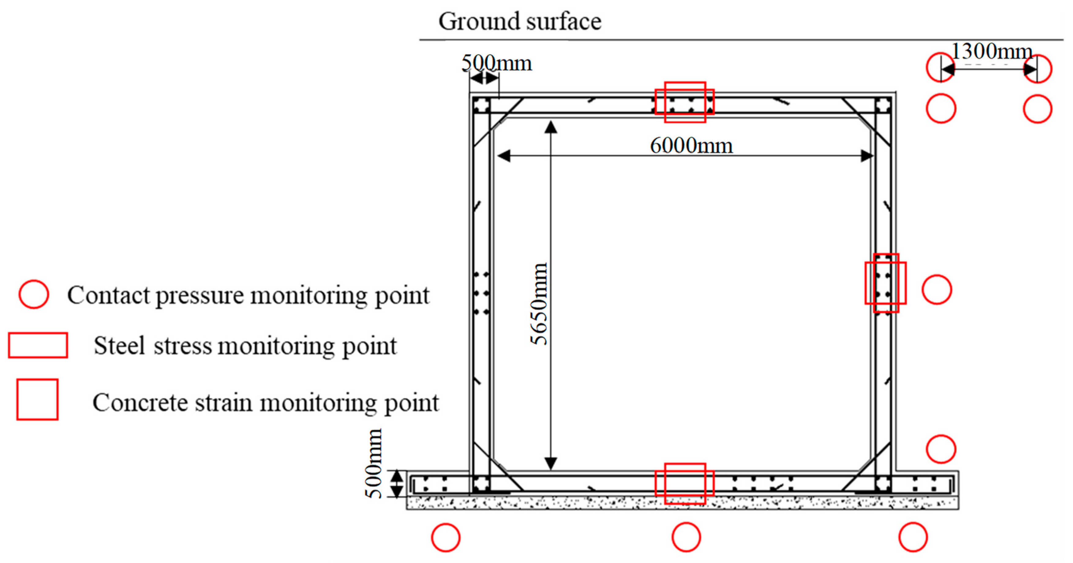
For a complex structure of a DBN which is composed of multiple-layer RBMs, there are many hyperparameters in the DBN that should be determined beforehand. Generally, those hyperparameters are determined by the control variable method. However, using the control variable method, there are three main shortcomings [31], which are as follows: (1) For many search parameters, it is hard work to implement a control variable method. (2) For a small search range, the searched optimal value is only the result in this small range, rather than the real optimal one. (3) The theoretical basis of the control variable method is lacking. To solve those shortcomings, it is a very suitable way to use the optimization method to select the suitable hyperparameters of a DBN. As one good global optimization method, the WOA can be used to select the optimal hyperparameters of the machine learning model [33]. Therefore, in this study, the WOA is used to determine the suitable hyperparameters of the DBN, and a new deep learning model called a whale optimization deep belief network (WO-DBN) is proposed, whose flow chart is shown in Figure 6.

It must be noted that, in this deep learning model, based on the experience and our tests, there are four hidden layers. The ReLU activation function, which only requires a threshold to obtain the activation value and has a very fast convergence speed, is used [34].

The main steps of the new deep learning model are as follows:

(1) Based on the experience, the searched ranges of the DBN hyperparameters that should be determined are provided. The hyperparameters include the neuron numbers for the first, second, third and fourth hidden layers (n₁, n₂, n₃ and n₄), the learning rate η and the maximum iteration numbers for pre-training and fine-tuning (T₁ and T₂), which are taken as the whale position $\overrightarrow{Z}$, represented as,

$$\overrightarrow{Z}=\left[n_1,n_2,n_3,n_4,\eta ,T_1,T_2\right],$$

(15)

(2) Based on the experiments and our tests, the initial parameters of the WOA are given, including the maximum iteration number T_max, the whale population size N and the spiral size constant b. According to the number of optimized hyperparameters, the dimension D is determined to be 7. Moreover, the initial whale population is generated randomly.

(3) According to the solved problem, the fitness function is defined as

$$f=\frac{{\displaystyle \sum _{i=1}^M{\left(y_i-y_i^{\prime }\right)}^2}}{M},$$

(16)

where $y_i^{\prime }$ and $y_i$ are the computed and real values of the ith sample, respectively, and M is the number of samples.

By using this fitness function, the fitness values of whale individuals can be obtained. According to its fitness value, the most adaptive individual is taken as the prey, whose position is selected as the target position.

(4) Based on the computing operations in the fourth step of the WOA, the positions of whale individuals have been updated, and the new whale population is generated.

(5) If the iteration number reaches the maximum iteration number T_max, the process is over. Otherwise, the process returns to step (3).

(6) The whale individual with the best position is selected and outputted, whose position is the optimized DBN hyperparameters. And by using those hyperparameters, the suitable DBN model can be obtained.

2.4. Filed Test

The utility tunnel engineering is in the high-speed railway business district of Suqian City, Jiangsu Province of China. For this engineering, one section is along the Guangzhou Road, whose width is 40 m and length is 1851 m. The single cabin structure of this utility tunnel should meet the entering requirement of power, communication and water supply pipelines in the tunnel. The utility tunnel is under the central green isolation zone, as shown in Figure 7.

For this utility tunnel engineering, the main tunnel structure is constructed by the segmented open excavation and cast-in-place and is one long strip single-cabin-reinforced concrete structure. The length of one segment is 25 m. The width and height of a standard section for this utility tunnel structure are 3 m and 3.5 m, and those for the directly buried outlet shaft are 6 m and 5.65 m. For a large size and complex structure for the section of the directly buried outlet shaft, in this study, the utility tunnel of the directly buried outlet shaft between the pile number of GZK 0 + 820 to GZK 0 + 900 is selected as the research object. For this utility tunnel of the directly buried outlet shaft, the covered depth is only about 2 m.

The site of this utility tunnel engineering belongs to the Xuhuai Yellow River alluvial plain geomorphic area, which is a unit of the abandoned ancient Yellow River channel geomorphology and has a flat terrain. By using the geological investigation method, such as the drilling method, in the report of engineering geological exploration, the engineering geological cross-section of this utility tunnel engineering can be obtained, which is shown in Figure 8.

From Figure 8 and according to the report of engineering geological exploration, there are six soil layers, for which the basic engineering geological conditions are summarized as follows.

For layer 1, it is the plain fill soil layer with the color of yellow or grayish yellow, it is loose and its main composition is silt, including the plant roots and stems, and locally contains crushed stones, bricks, etc. For its poor mechanical properties, this layer has been removed.

For layer 2-1, it is the silt layer with the color of grayish yellow, and it is wet and slightly dense. For this layer, the thin layers of soft plastic clay are mixed in local layers, and there is a feeling of sand when rubbing hands with a rapid shaking response. This layer has low toughness and dry strength with moderate compressibility.

For layer 2-2, it is the clay layer, whose color is from grayish brown to yellowish gray with soft plastic and local plastic. For this layer, the thin layers of silt are partially mixed with the glossy cut surface. Moreover, this soil layer has high toughness and dry strength, with no shaking response and medium to high compressibility.

For layer 2-2A, it is the sullage silty clay layer, whose color is from grayish brown to yellowish gray, too. For this layer with a mechanical property from soft plastic to flow plastic, the thin layers of silt are also mixed with the slight glossy cut surface. Moreover, this soil layer has medium toughness and dry strength, with no shaking response and high compressibility.

For layer 2-3, which is the clay layer whose color is grayish brown or yellowish gray, it is from soft to plastic, with the glossy cut surface including a small number of iron manganese spots. This layer has high toughness and dry strength with no shaking response and medium compressibility.

For layer 2-4, it is the silty clay layer whose color is from gray yellow to brown yellow, and the mechanical property is from plastic to hard plastic. Moreover, the local layers of this layer are clay including iron manganese spots and a small number of calcareous nodules. As for layer 2-3, this layer has high toughness and dry strength, with no shaking response and medium compressibility, too.

From the above analysis, it can be found that, for the soil layers in which the utility tunnel is located, there are mainly two parts, which are soft soil in lower layers and filling soil in upper layers. The soft soil layers mainly include the sullage silty clay and the silty clay. Therefore, the soil layers in which the utility tunnel is located belongs to the typical soft soil.

Because the utility tunnel engineering, which is a typical soft foundation engineering, is shallowly buried under the green isolation areas, it will be seriously affected by the ground traffic load during the operation period, which will cause large deformation for the utility tunnel. Moreover, for locations near multiple ground transportation routes, this engineering will be repeatedly affected by the loads of incoming and outgoing ground vehicles. Therefore, for this utility tunnel engineering with its big size and complex structure during the operation period, the ground traffic load will significantly influence its safety. It is very important work to monitor and predict the safety for this utility tunnel during the operation period.

To monitor the response of the utility tunnel structure during the operation period in-site, the steel stress gauge and concrete strain gauge are placed at the middle of the floor, the side wall and the roof of the structure for the directly buried outlet shaft. Moreover, the contact pressure monitoring sensors are embedded in soil at different depths along the side wall of the utility tunnel and along the floor. The layout of field monitoring points is shown in Figure 9.

In this study, the used data acquisition instrument is the dynamic and static signal testing system of Chentu CT5808W, whose adjustable maximum frequency is 50 Hz. This instrument can capture the slight changes in sensors within a short period of time. In the field test, to simulate the vehicle load under normal two-way traffic and one-way traffic conditions, on the second lane from east to west and the opposite lane, vehicle load action tests have been conducted, with rear axle loads of 8.3 tons, 9 tons and 11 tons. The vehicle load, which is a one-time action, is applied by a dump truck.

3. Results

3.1. Construction Datasets from Field Tests Results

From the field test, it can be found that the sensors buried in the roof of the structure can obviously reflect the disturbance of vehicle loads during the operation period. Therefore, the results of those sensors are used in this study. From the comprehensive analysis of the engineering condition, site investigation and real measurement data, it can be found that the main load disturbance factors affecting the response of the utility tunnel structure include the vehicle driving speed, the magnitude of the vehicle load, the lateral distance between the vehicle wheel load center and the mid span of the structure roof, the symmetry of the vehicle load distribution and the operating time. The disturbance response of the utility tunnel structure is mainly represented by the settlement and the horizontal stress at the mid span of the structure roof. It must be noted that the settlement of the mid span of the structure roof can be computed by the obtained concrete strain results at the corresponding position, and the horizontal stress at the mid span of the structure roof is also computed by the obtained steel stress results at the corresponding position. Therefore, to predict the safety of the utility tunnel structure, the four vehicle operating load parameters and one operating time parameter are selected as the influence factors, which are the input variables of the prediction model, and the response factors of the utility tunnel structure are the settlement and the horizontal stress at the mid span of the structure roof, which are the output variables of the prediction model. According to the requirements for the input and output variables of the prediction model, field test data have been organized to establish the datasets for the training the model. For the large number of field test datasets, in order to illustrate the form of the dataset, only part of the data are provided here, as shown in

Table 1. Part data of field test datasets.

Input Variables					Output Variables
Operating Time /h	Vehicle Speed /km/h	Symmetry of Vehicle Load	Magnitude of Vehicle Load /kN	Load Position /m	Vertical Displacement /mm	Horizontal Stress /kPa
1	22.5	1	156.49	5.25	2.0053	720.342
1.6	41.25	1	169.17	5.25	2.2926	730.722
2.17	60	1	190.01	5.25	2.2596	725.702
1.26	60	1	195.81	5.25	2.4146	728.099
4.31	41.25	1	180.01	5.25	2.0452	720.963
4.63	80	2	90.01	6.39	1.8	391.573
1.17	41.25	2	81.25	7.34	1.17	303.95
4.06	80	2	100.1	6.39	2.24	383.41
1.25	80	2	96.58	6.39	2.76	340.47
1	41.25	2	96.58	7.34	2.16	288.28

.

It must be noted that, in Table 1, the “1” in the third column represents load symmetry, and “2” represents load asymmetry. For the data in each line, the first five ones represent the five disturbance factors, and the last two represent the two corresponding responses of the utility tunnel structure affected by the first five disturbance factors. The data in each line are one training sample of the prediction model, and the datasets of the prediction model are constructed by numerous lines of the training sample.

Finally, it must be noted that, because the load disturbance factors can be determined easily in the field tests at one engineering site, in this study, only the main load disturbance factors have been considered. Actually, in real engineering, there are other influence factors on the performance of the utility tunnel structure, such as the type of soft foundation soil. However, those factors are unchanged for one particular utility tunnel during the operation period. Therefore, those influence factors cannot be taken as the disturbance factors for one particular form of engineering. Moreover, for one particular utility tunnel, the influence of the type of soft foundation soil has been represented in the implicit relationship between the load disturbance factors and structural responses. Therefore, for this prediction study, the influence of the type of soft foundation soil is not considered. That is to say, the type of soft foundation soil does not affect the predictive accuracy of the deep learning model.

3.2. Process of Prediction by WO-DBN

The prediction process of the settlement and the horizontal stress at the mid span of the structure roof based on WO-DBN is shown in Figure 10.

From Figure 10, the computing process of the prediction structure response of the utility tunnel is as follows.

(1) Based on the field test results, the datasets for the safety prediction model of the utility tunnel structure during the operation period have been constructed, that is, the field test datasets for the response of the utility tunnel structure during the operation period (including the structure deformation index data and structure stress index data) have been selected. Here, the field test data of a one-year simulated operation period have been used.

(2) The field test datasets have been preprocessed. The duplicate data and obvious abnormal data have been removed. The zero values in the datasets have been revised to the very small values (greater than zero). After preprocessing, a total of 15,376 sets of valid data have been obtained.

It should be noted that, if the amount of training data is very huge, to reduce the workload of processing the training data, the digital signal processing methods such as the wavelet analysis or filtration methods can be employed to optimize the selection and preprocessing of training data.

(3) Considering the total amount of data, the datasets have been divided. Approximately 80% of the data have been selected as the training sets, including a total of 12,110 sets, and the remaining data are as the testing sets. The used datasets are summarized in

Table 2. The used datasets.

Name	Field Test Datasets	Training Sets	Testing Sets
Number of sets	15,376	12,110	3266

.

(4) The hyperparameters of the DBN have been optimized by the WOA, and the prediction model by the DBN based on the optimization results has been established. The predication model has been trained by the training sets to determine the parameters of the predication model, and the WO-DBN model for the prediction of the vertical displacement and the horizontal stress at the mid span of the structure roof can be obtained.

(5) The data of the load and operating time of the testing sets have been substituted into the obtained WO-DBN model, and the corresponding structure response can be obtained, which are the predicted results of the vertical displacement and the horizontal stress at the mid span of the structure roof.

3.3. Evaluation Index of the Prediction Model

In this study, the square root mean square error (RMSE), mean absolute error (MAE) and correlation coefficient (R) are used to evaluate the prediction accuracy of the model, which are as follows:

$$\mathrm{RMSE}=\sqrt{\frac{{\displaystyle \sum _{i=1}^N{\left(y_i-y_i^{\prime }\right)}^2}}{N}},$$

(17)

$$\mathrm{MAE}=\frac{{\displaystyle \sum _{i=1}^N\left|y_i-y_i^{\prime }\right|}}{N},$$

(18)

$$\mathrm{R}=\frac{{\displaystyle \sum _{i=1}^N(y_i-\overline{y})(y_i^{\prime }-\overline{y^{\prime }})}}{\sqrt{{\displaystyle \sum _{i=1}^N{(y_i-\overline{y})}^2}{\displaystyle \sum _{i=1}^N{(y_i^{\prime }-\overline{y^{\prime }})}^2}}},$$

(19)

where $y_i^{\prime }$ represents the prediction value corresponding to the i-th input data, $\overline{y^{\prime }}$ represents the average value of prediction values, $y_i$ represents the real test value corresponding to the i-th input data, $\overline{y}$ represents the average value of real test values and N represents the number of prediction samples.

3.4. Analysis of Predication Results

The training sets are used to train the predication model, and the WO-DBN model can be obtained. The optimized hyperparameters of the DBN, which are the parameters of the WO-DBN, are summarized in

Table 3. Parameters of the WO-DBN model.

Parameters	n1	n2	n3	n4	η	t1	t2
Values	44	47	34	18	0.0044	13	60

.

The testing sets have been substituted into the obtained WO-DBN model, and the prediction results of the structure response can be obtained, which are as shown in Figure 11. It must be noted that, for comparison, the real test results are also shown in this figure.

It must be noted that, in Figure 11, to show the computing errors between the prediction results and the real test ones clearly, the scattered points of vertical displacement and the horizontal stress of the structure roof corresponding to different samples were artificially connected to form variation curves. Therefore, the variation curves in Figure 11 have no practical meaning.

From Figure 11, it can be found that the prediction results of the WO-DBN model are in agreement with the real test results—that is, the performance of the constructed prediction model in this study is suitable.

To deeply analyze the prediction results, based on Equations (17)–(19), the quantitative evaluation indexes (RMSE, MAE and R) can be obtained, which are summarized in

Table 4. Evaluation indexes of the WO-DBN prediction model.

Indexes	RMSE	MAE	R
Vertical Displacement	0.2312	0.1604	0.9742
Horizontal stress	22.0217	12.3726	0.6825

.

From Table 4, it can be found that, for the vertical displacement of the structure roof, the values of RMSE and MAE are all small, and the value of R is 0.9742, which is near 1. Therefore, the prediction results are very good. However, for the horizontal stress of the structure roof, the values of RMSE and MAE are large. The reason is that the computing values of RMSE and MAE are related with the magnitude of the data [27,35]. Because the magnitude of the data for the horizontal stress is much larger than that for the vertical displacement, there are big differences for the computing values of RMSE and MAE between them. Moreover, the computing value of R is not related with the magnitude of the data [27,35]. Therefore, its result is relatively effective. Actually, for the horizontal stress of the structure roof, its computing value of R is 0.6825, which is near 0.7, that is, the prediction result of WO-DBN is somewhat suitable too. Obviously, the prediction result of vertical displacement is better than that of horizontal stress, that is, the obtained WO-DBN prediction model has a better predictive effect on the structure deformation response. The reason is that the displacement response of the utility tunnel structure to the disturbances such as operation loads is more obvious than the stress response, which is represented by the more obvious change in results in Figure 11a than that in Figure 11b.

From the above analysis, it can be found that, based on the constructed WO-DBN model and considering the disturbance factors of the utility tunnel structure during the operation period, the corresponding disturbance response of the utility tunnel structure can be predicted well. Therefore, this study can provide an effective way to dynamically predict the safety response of the utility tunnel structure during the operation period based on the big data analysis by the artificial intelligent method.

4. Discussion

To further analyze the performance of the WO-DBN model, a comparison study between WO-DBN, DBN, ANN and another deep learning method called long short-term memory (LSTM) has been conducted.

For the DBN model, the trial-and-error method is generally used to determine its hyperparameters, which can be described as follows.

(1) According to the experience, the possible ranges of hyperparameters have been determined.

(2) Several sets of hyperparameter combinations have been selected in their possible ranges by the experimental design or other methods, and these hyperparameter combinations have been used for prediction.

(3) The prediction errors of models by the different combinations of hyperparameters have been used for comparison, that is, the evaluation indexes of the prediction models have been compared. The parameter combination with the smallest prediction error has been selected as the final hyperparameters of the prediction model.

By using the trial-and-error method, the determined hyperparameters of the DBN model are summarized in

Table 5. Parameters of the DBN model.

Parameters	n1	n2	n3	n4	η	t1	t2
Values	45	50	30	10	0.0014	15	65

.

As one typical artificial intelligence method, the ANN is generally used for prediction study [27,35,36,37]. Therefore, it is used here for comparison. By using the trial-and-error method, too, its hyperparameters can be determined, which are summarized in

Table 6. Parameters of the ANN and LSTM models.

	Parameters	n1	n2	η	Epoch
ANN	Values	32	16	0.01	50
LSTM	Values	16	8	0.001	100

.

It should be noted that, in Table 6, n₁ and n₂ are neuron numbers for the first and second hidden layers, respectively. η is the learning rate, and Epoch is the maximum iteration number.

Moreover, for the LSTM which belongs to the recurrent neural network (RNN) [38], it is one generally used deep learning method for the prediction study [38,39]. Therefore, here, for a comparison with the new deep learning model (WO-DBN), the LSTM is applied. By using the trial-and-error method, the hyperparameters of LSTM can also be determined. Because the determined structure of LSTM is the same as that of ANN, the hyperparameters of LSTM are also summarized in Table 6.

By using the determined parameters in Table 5 and Table 6, the prediction models for the response of the utility tunnel structure based on DBN, ANN and LSTM can be constructed. For comparison, the prediction results of the DBN, ANN and LSTM models are also shown in Figure 11. From Figure 11, it can be found that there are some differences between the prediction results of the three models (DBN, ANN and LSTM) and the real test results, and the results of WO-DBN approach the real data more. Therefore, the prediction results of the new WO-DBN model are the best, which are much better than those of the three models. Moreover, to compare the four models (WO-DBN, DBN, ANN and LSTM) more clearly, the quantitative evaluation indexes (RMSE, MAE and R) of the four prediction models are summarized in

Table 7. Comparison of evaluation indexes for four prediction models (WO-DBN, DBN, ANN and LSTM).

		WO-DBN	DBN	ANN	LSTM
Vertical displacement	RMSE	0.2312	0.5697	0.6563	0.5595
	MAE	0.1604	0.4285	0.4852	0.3777
	R	0.9742	0.8642	0.7585	0.8435
Horizontal stress	RMSE	22.0217	31.2888	38.1835	34.5109
	MAE	12.3726	24.7234	30.4551	28.2891
	R	0.6825	0.5011	0.3411	0.5145

.

From Table 7, it can be found that, both for the vertical displacement and for the horizontal stress, the computing errors of the WO-DBN model are all much less than those of the three other models (DBN, ANN and LSTM). For example, the R for the vertical displacement by WO-DBN is 0.9742, which is much larger than those by DBN (0.8642), ANN (0.7585) and LSTM (0.8435). The R for the horizontal stress by WO-DBN is 0.6825, which is also much larger than those by DBN (0.5011), ANN (0.3411) and LSTM (0.5145). Therefore, the performance of the prediction model by WO-DBN is significantly better than those by DBN, ANN and LSTM. The proposed WO-DBN model is a more suitable method for predicting the performance of the utility tunnel structure during the operation period. Moreover, in four prediction models, the performance of ANN is the poorest, whose computed R for the vertical displacement and the horizontal stress is the least. The computed R for the vertical displacement by DBN is larger than that by LSTM, but the computed R for the horizontal stress by DBN is slightly less than that by LSTM. However, with comprehensive consideration of the computing errors, the performance of DBN is superior. Therefore, for the prediction of the performance of the utility tunnel structure during the operation period, the order of the four models is as follows: WO-DBN, DBN, LSTM and ANN.

Although the proposed WO-DBN model can well predict the performance of the utility tunnel structure in a soft foundation during the operation period and its performance is much better than that of other models (DBN, ANN and LSTM), as a preliminary study, the amount of used data is not very large, and the considered structure disturbance factors are not very comprehensive. Moreover, in this deep learning model, the WOA is only used to select the hyperparameters of the DBN, and the DBN is still trained by the traditional greedy layer-by-layer learning algorithm. Finally, in this study, the offline data are used in the prediction model, which restricts the real-time prediction. Therefore, the future works can be summarized as follows: (1) a prediction study on the real big data of the measured disturbance of the utility tunnel structure during the operation period, (2) a prediction study considering more structure disturbance factors for the utility tunnel structure during the operation period, (3) the development of a new deep learning model, in which both the hyperparameters and algorithm parameters of DBN are all optimized by the WOA and (4) a prediction study based on the real-time monitoring data to enhance the predictive capabilities of the deep learning model.

5. Conclusions

In this study, to monitor the performance of the utility tunnel structure in a soft foundation affected by ground traffic loads during the operation period, the field tests have been conducted in the typical engineering site (one utility tunnel engineering in Suqian City of Jiangsu Province, China). From the field test results, the five main disturbance factors (four vehicle operating load parameters and one operating time parameter) on the utility tunnel structure and the two main structural safety responses (displacement and stress) have been determined to construct the big datasets whose number is 15,376 for the prediction model. To treat the datasets, one new deep learning model called WO-DBN has been proposed, in which the WOA is used to optimize the hyperparameters of the DBN. Finally, using the WO-DBN model, and based on the datasets, the main safety responses of the utility tunnel structure have been predicted. From the studies, the following conclusions can be drawn: (1) For the utility tunnel structure in a soft foundation during the operation period, the two main safety responses affected by the five main disturbance factors such as the load and time are the displacement and stress at the mid span of the structure roof. (2) For its special structure and good computing performance, the deep learning method (DBN) can analyze the big data from the field tests well; however, for the numerous hyperparameters of DBN, which cannot be determined easily, the WOA is used to optimize those hyperparameters, and a new deep learning model (WO-DBN) is proposed to treat the big data. (3) Based on the new WO-DBN model, the dynamic safety status of the utility tunnel structure in a soft foundation during the operation period can be predicted well, whose results show that the computing errors are not significant (the average absolute error for the displacement is 0.1604 and that for the stress is 12.3726) and can meet the requirement of real engineering.

References

1. Luo, Y.; Alaghbandrad, A.; Genger, T.; Hammad, A. History and recent development of multi-purpose utility tunnels. Tunn. Undergr. Space Technol. 2020, 103, 103511. [Google Scholar] [CrossRef]
2. Yang, C.; Peng, F.-L. Discussion on the Development of Underground Utility Tunnels in China. Procedia Eng. 2016, 165, 540–548. [Google Scholar] [CrossRef]
3. Zhou, Q.; He, H.; Liu, S.; Wang, P.; Zhou, Y.; Zhou, J.; Fan, H.; Jin, F. Evaluation of blast-resistant ability of shallow-buried rein-forced concrete urban utility tunnel. Eng. Fail. Anal. 2021, 119, 105003. [Google Scholar] [CrossRef]
4. Zhou, Q.; He, H.-G.; Liu, S.-F.; Chen, X.-S.; Tang, Z.-X.; Liu, Y.; Qiu, Z.-Y.; Li, S.-S.; Wang, H.; Zhou, Y.-Z.; et al. Blast resistance evaluation of urban utility tunnel reinforced with BFRP bars. Def. Technol. 2020, 17, 512–530. [Google Scholar] [CrossRef]
5. Pan, Y.; Zong, Z.; Li, J.; Qian, H.; Wu, C. Investigating the dynamic response of a double-box utility tunnel buried in calcareous sand against ground surface explosion. Tunn. Undergr. Space Technol. 2024, 146, 105636. [Google Scholar] [CrossRef]
6. Zhao, G.; Zhu, L.; Wu, S.; Liu, W.; Duan, S. Experimental and numerical investigation on the cross-sectional mechanical behavior of prefabricated multi-cabin RC utility tunnels. Structures 2022, 42, 466–479. [Google Scholar] [CrossRef]
7. Zhang, J.; Zhang, Y.; Peng, C.; Lei, Y.; Zhang, A.; Zuo, Z.; Chen, Z. Experimental and Numerical Investigation into Full-Scale Model of New Type Assembled Integral Utility Tunnel. Buildings 2023, 13, 1428. [Google Scholar] [CrossRef]
8. Xue, W.; Chen, S.; Wang, Q. Cyclic Loading Test Conducted on the Bottom Joints of a Hybrid Precast Utility Tunnel Composed of Double-Skin Sidewalls and a Precast Bottom Slab. Buildings 2024, 14, 341. [Google Scholar] [CrossRef]
9. Zhong, Z.; Li, G.; Li, J.; Shen, J.; Zhao, M.; Du, X. Experimental study on out-of-plane seismic performance of precast composite sidewalls of utility tunnel with grouting-sleeve joints. Undergr. Space 2024, 16, 1–17. [Google Scholar] [CrossRef]
10. Xue, W.; Chen, S.; Bai, H. Pseudo-Static Tests on Top Joints of Hybrid Precast Utility Tunnel. Buildings 2023, 13, 2567. [Google Scholar] [CrossRef]
11. Chen, H.; El Naggar, M.H.; Chu, J.; Li, X.; He, Q.; Wang, L.; Liu, X.; Zhou, L. Transverse response of utility tunnel under near fault ground motions: Multi-shake table array tests. Soil Dyn. Earthq. Eng. 2023, 174, 108135. [Google Scholar] [CrossRef]
12. Yue, F.; Liu, B.; Zhu, B.; Jiang, X.; Chen, S.; Jaisee, S.; Chen, L.; Lv, B. Shaking table investigations on seismic performance of prefabricated corrugated steel utility tunnels. Tunn. Undergr. Space Technol. 2020, 105, 103579. [Google Scholar] [CrossRef]
13. Yao, A.; Tian, T.; Gong, Y.; Li, H. Shaking Table Tests of Seismic Response of Multi-Segment Utility Tunnels in a Layered Liquefiable Site. Sustainability 2023, 15, 6030. [Google Scholar] [CrossRef]
14. Liang, J.; Zhang, J.; Dong, B.; Xu, A.; Ba, Z. Shaking table tests on the seismic performance of prefabricated T-shaped cross utility tunnel. Structures 2023, 58, 105516. [Google Scholar] [CrossRef]
15. Huang, D.-L.; Zong, Z.-L.; Tao, X.-X.; Liu, Q.; Huang, Z.-Y.; Tang, A.-P. Seismic response of utility tunnel in horizontal nonhomogeneous site based on improved discrete element method. Structures 2023, 57, 105179. [Google Scholar] [CrossRef]
16. Yue, F.; Liu, B.; Zhu, B.; Jiang, X.; Chen, L.; Liao, K. Shaking table test and numerical simulation on seismic performance of prefabricated corrugated steel utility tunnels on liquefiable ground. Soil Dyn. Earthq. Eng. 2020, 141, 106527. [Google Scholar] [CrossRef]
17. Tsinidis, G. Response characteristics of rectangular tunnels in soft soil subjected to transversal ground shaking. Tunn. Undergr. Space Technol. 2017, 62, 1–22. [Google Scholar] [CrossRef]
18. Zhang, Y.; Liu, B.; Meng, L. Structural behavior and soil arching state of underground corrugated steel utility tunnel. J. Constr. Steel Res. 2023, 203, 107798. [Google Scholar] [CrossRef]
19. Huang, B.-T.; Zhu, J.-X.; Weng, K.-F.; Huang, J.-Q.; Dai, J.-G. Prefabricated UHPC-concrete-ECC underground utility tunnel reinforced by perforated steel plate: Experimental and numerical investigations. Case Stud. Constr. Mater. 2022, 16, e00856. [Google Scholar] [CrossRef]
20. Huang, Z.; Feng, Y.; Tang, A.; Liu, Q. Influence of oblique incidence of P-waves on seismic response of prefabricated utility tunnels considering joints. Soil Dyn. Earthq. Eng. 2023, 167, 107797. [Google Scholar] [CrossRef]
21. Qian, H.; Zong, Z.; Wu, C.; Li, J.; Gan, L. Numerical study on the behavior of utility tunnel subjected to ground surface explosion. Thin-Walled Struct. 2021, 161, 107422. [Google Scholar] [CrossRef]
22. Yin, X.; Liu, H.; Chen, Y.; Wang, Y.; Al-Hussein, M. A BIM-based framework for operation and maintenance of utility tunnels. Tunn. Undergr. Space Technol. 2020, 97, 103252. [Google Scholar] [CrossRef]
23. Yang, L.; Zhang, F.; Yang, F.; Qian, P.; Wang, Q.; Wu, Y.; Wang, K. Generating Topologically Consistent BIM Models of Utility Tunnels from Point Clouds. Sensors 2023, 23, 6503. [Google Scholar] [CrossRef]
24. Peng, F.-L.; Qiao, Y.-K.; Yang, C. A LSTM-RNN based intelligent control approach for temperature and humidity environment of urban utility tunnels. Heliyon 2023, 9, e13182. [Google Scholar] [CrossRef]
25. Wu, J.; Bai, Y.; Fang, W.; Zhou, R.; Reniers, G.; Khakzad, N. An Integrated Quantitative Risk Assessment Method for Urban Underground Utility Tunnels. Reliab. Eng. Syst. Saf. 2021, 213, 107792. [Google Scholar] [CrossRef]
26. Xue, G.; Liu, S.; Ren, L.; Gong, D. Risk assessment of utility tunnels through risk interaction-based deep learning. Reliab. Eng. Syst. Saf. 2024, 241, 109626. [Google Scholar] [CrossRef]
27. Ansari, A.; Rao, K.; Jain, A.; Ansari, A. Formulation of multi-hazard damage prediction (MhDP) model for tunnelling projects in earthquake and landslide-prone regions: A novel approach with artificial neural networking (ANN). J. Earth Syst. Sci. 2023, 132, 164. [Google Scholar] [CrossRef]
28. Liu, W.; Wang, Z.; Liu, X.; Zeng, N.; Liu, Y.; Alsaadi, F.E. A survey of deep neural network architectures and their applications. Neurocomputing 2017, 234, 11–26. [Google Scholar] [CrossRef]
29. Gong, B.; Shu, C.; Han, S.; Cheng, S.-G. Mine Vegetation Identification via Ecological Monitoring and Deep Belief Network. Plants 2021, 10, 1099. [Google Scholar] [CrossRef]
30. Zhou, C.; Gao, W.; Cui, S.; Zhong, X.; Hu, C.; Chen, X. Ground Settlement of High-Permeability Sand Layer Induced by Shield Tunneling: A Case Study under the Guidance of DBN. Geofluids 2020, 2020, 6617468. [Google Scholar] [CrossRef]
31. Hinton, G.E.; Osindero, S.; Teh, Y.-W. A Fast Learning Algorithm for Deep Belief Nets. Neural Comput. 2006, 18, 1527–1554. [Google Scholar] [CrossRef]
32. Mirjalili, S.; Lewis, A. The whale optimization algorithm. Adv. Eng. Softw. 2016, 95, 51–67. [Google Scholar] [CrossRef]
33. Zhou, J.; Zhu, S.; Qiu, Y.; Armaghani, D.; Zhou, A.; Yong, W. Predicting tunnel squeezing using support vector machine opti-mized by whale optimization algorithm. Acta Geotech. 2022, 17, 1343–1366. [Google Scholar] [CrossRef]
34. Krizhevsky, A.; Sutskever, I.; Hinton, G.E. Imagenet classification with deep convolutional neural networks. Commun. ACM 2017, 60, 84–90. [Google Scholar] [CrossRef]
35. Ahmad, S.A.; Ahmed, H.U.; Rafiq, S.K.; Ahmad, D.A. Machine learning approach for predicting compressive strength in foam concrete under varying mix designs and curing periods. Smart Constr. Sustain. Cities 2023, 1, 16. [Google Scholar] [CrossRef]
36. Nguyen, L.Q.; Le, T.T.T.; Nguyen, T.G.; Tran, D.T. Prediction of underground mining-induced subsidence: Artificial neural network based approach. Min. Miner. Depos. 2023, 17, 45–52. [Google Scholar] [CrossRef]
37. Kim, Y.; Lee, S.S. Application of Artificial Neural Networks in Assessing Mining Subsidence Risk. Appl. Sci. 2020, 10, 1302. [Google Scholar] [CrossRef]
38. Yang, T.; Wen, T.; Huang, X.; Liu, B.; Shi, H.; Liu, S.; Peng, X.; Sheng, G. Predicting Model of Dual-Mode Shield Tunneling Parameters in Complex Ground Using Recurrent Neural Networks and Multiple Optimization Algorithms. Appl. Sci. 2024, 14, 581. [Google Scholar] [CrossRef]
39. He, Y.; Chen, Q. Construction and Application of LSTM-Based Prediction Model for Tunnel Surrounding Rock Deformation. Sustainability 2023, 15, 6877. [Google Scholar] [CrossRef]
Figure 1. Structure of the DBN.
Applsci 14 02334 g001
Figure 2. Structure of the RBM.
Applsci 14 02334 g002
Figure 3. Training process of the DBN.
Applsci 14 02334 g003
Figure 4. Flow chart of the greedy layer-by-layer learning algorithm.
Applsci 14 02334 g004
Figure 5. Flow chart of the WOA.
Applsci 14 02334 g005
Figure 6. Flow chart of the WO-DBN.
Applsci 14 02334 g006
Figure 7. Layout of the utility tunnel.
Applsci 14 02334 g007
Figure 8. Cross-section of engineering geology.
Applsci 14 02334 g008
Figure 9. Layout of monitoring points.
Applsci 14 02334 g009
Figure 10. Flow chart of the prediction structure response of the utility tunnel based on WO-DBN.
Applsci 14 02334 g010
Figure 11. Prediction results of the structure response for the utility tunnel: (a) Vertical displacement at the mid span of the structure roof; (b) Horizontal stress at the mid span of the structure roof.
Applsci 14 02334 g011