NSVDNet: Normalized Spatial-Variant Diffusion Network for Robust Image-Guided Depth Completion

Abstract

Depth images captured by low-cost three-dimensional (3D) cameras are subject to low spatial density, requiring depth completion to improve 3D imaging quality. Image-guided depth completion aims at predicting dense depth images from extremely sparse depth measurements captured by depth sensors with the guidance of aligned Red–Green–Blue (RGB) images. Recent approaches have achieved a remarkable improvement, but the performance will degrade severely due to the corruption in input sparse depth. To enhance robustness to input corruption, we propose a novel depth completion scheme based on a normalized spatial-variant diffusion network incorporating measurement uncertainty, which introduces the following contributions. First, we design a normalized spatial-variant diffusion (NSVD) scheme to apply spatially varying filters iteratively on the sparse depth conditioned on its certainty measure for excluding depth corruption in the diffusion. In addition, we integrate the NSVD module into the network design to enable end-to-end training of filter kernels and depth reliability, which further improves the structural detail preservation via the guidance of RGB semantic features. Furthermore, we apply the NSVD module hierarchically at multiple scales, which ensures global smoothness while preserving visually salient details. The experimental results validate the advantages of the proposed network over existing approaches with enhanced performance and noise robustness for depth completion in real-use scenarios.

1. Introduction

Depth sensing and estimation are of vital importance in a wide range of applications, e.g., robotics [1], autonomous driving [2], and augmented reality [3]. However, depth sensors, such as Light Detection and Ranging (LiDAR) and Time-of-Flight (ToF) sensors, typically provide relatively low output density [4,5], as demonstrated in Figure 1b. This hinders the application of depth sensors in downstream applications that require dense depth maps.

To improve three-dimensional (3D) imaging quality, direct interpolation with only sparse depth measurements can efficiently provide a dense depth map [6] but results in blurry edges and structural details as shown in Figure 1c. On the other hand, Red–Green–Blue (RGB) cameras capture the high-resolution shape and structure information of the scene, and a cost-effective way to obtain dense depth is to estimate it directly from a single image based on monocular depth estimation algorithms [7,8]. However, the inference accuracy is relatively low and the generalization ability is limited, which restrict their applications in scenarios requiring high accuracy and robustness in depth estimation [9,10]. For example, in Figure 1d, although the monocular depth estimation is able to preserve the relative distance, it is hard to provide accurate absolute measurement [7]. This is consistent with the quantitative evaluation using the Root Mean Squared Error (RMSE) metric [11], where the result in Figure 1d shows a relatively larger RMSE indicating low accuracy. Therefore, existing approaches use RGB images as guidance to recover dense depth maps from sparse sensor depth measurements; this is called image-guided depth completion [4,11]. For example, with the RGB image input in Figure 1a as guidance, the structural details are better preserved to achieve improved accuracy as shown in Figure 1e.

Figure 1. Example in NYUv2 dataset [12]. (a) RGB image input, (b) sparse depth input, depth estimation with (c) PNCNN [6] using single depth, (d) MiDaS [7] using single RGB, (e) NLSPN [11], and (f) proposed NSVDNet using both RGB and depth. As highlighted in the black rectangles, (f) NSVDNet generates more accurate structural details than (e) NLSPN due to the uncertainty-aware diffusion scheme. The results are evaluated using RMSE metric, where (f) NSVDNet achieves the smallest RMSE, indicating improved accuracy.

Figure 1. Example in NYUv2 dataset [12]. (a) RGB image input, (b) sparse depth input, depth estimation with (c) PNCNN [6] using single depth, (d) MiDaS [7] using single RGB, (e) NLSPN [11], and (f) proposed NSVDNet using both RGB and depth. As highlighted in the black rectangles, (f) NSVDNet generates more accurate structural details than (e) NLSPN due to the uncertainty-aware diffusion scheme. The results are evaluated using RMSE metric, where (f) NSVDNet achieves the smallest RMSE, indicating improved accuracy.

In recent years, deep neural networks have achieved great success in various applications [1,4,13] and have been successfully applied in image-guided depth completion tasks, achieving remarkable improvements in depth estimation accuracy. Various network architectures have been proposed to integrate features from RGB and depth completion tasks [14,15]. The problem is, most depth completion approaches ignore the fact that the sensor depth is inherently noisy [16,17], and the performance will fail at inaccurate depth measurements.

To enhance the network robustness to input noise and guarantee reliability in real-world usage, increasing attention has been paid to incorporating prior knowledge about depth images into the network design [18,19]. In this way, the solution space of the network is restricted to avoid over-fitting to the training dataset, which in turn enhances the generalization ability to unseen real test data. However, the task of image-guided depth completion has not received enough attention in terms of network reliability, and the corruption in the input sparse sensor depth is not fully considered, which leads to degradation in the resulting depth prediction.

To tackle the above problems, we propose the normalized spatial-variant diffusion network (NSVDNet) based on uncertainty-aware diffusion to enhance performance robustness to input corruption. Specifically, the sparse depth is diffused with end-to-end learned spatially adaptive kernels that incorporate (1) the input depth uncertainty to avoid diffusing corrupted depth measurements and (2) the semantic features learned from RGB images to further enhance structural detail reconstruction. By utilizing the above uncertainty-aware diffusion, we essentially implemented anisotropic diffusion in the network, making the network interpretable and thus limiting the solution space to avoid over-fitting to the training dataset. This explains why the proposed NSVDNet is robust to the noise in corrupted input data that is not included in the training dataset.

To implement the uncertainty-aware diffusion on depth maps, we design the normalized spatial-variant diffusion (NSVD) module utilizing the learned depth certainty as a normalization factor to mitigate depth noise, and the spatial-variant affinity extracted from RGB to guide structural enhancement. Furthermore, the NSVD module is applied hierarchically at multiple scales so as to ensure global smoothness while preserving visually salient details.

In sum, previous approaches for depth completion can be classified into three categories: (1) modifying convolution layers to adapt to sparse input [20]; (2) utilizing RGB-D fusion to recover dense depth with RGB guidance [14,15]; and (3) constructing affinity matrices to refine structural details [11]. However, when the input depth measurements are corrupted [16,17], the extracted features do not unveil the underlying structure of the depth, which degrades the resulting depth estimation for these schemes. In contrast, the proposed NSVDNet provides the following advantages over existing schemes: (1) NSVDNet utilizes uncertainty-aware diffusion to enhance the network robustness to input corruption based on the input depth uncertainty; (2) NSVD modules are applied hierarchically to the depth features to further enhance the RGB-D fusion efficiency; (3) NSVDNet essentially implements anisotropic diffusion, which limits the solution space to avoid over-fitting and enhance generalization ability. More discussions about the comparison with existing schemes are provided in Section 2. The example in Figure 1f shows that the proposed NSVDNet outperforms the competing scheme NLSPN [11] where the global smoothness and local detail are better preserved without introducing extra textures, e.g., on the bicycle and the table corner highlighted in the black rectangles. Also, the result in Figure 1f shows a smaller RMSE value than that in Figure 1e, validating the enhanced accuracy of NSVDNet. In summary, the main contributions of our work include:

• We design the uncertainty-aware diffusion network to enhance the robustness to depth measurement corruption, where the input depth uncertainty is integrated into the diffusion to avoid input noise from propagating to neighboring pixels;
• We implement the diffusion with the normalized spatial-variant diffusion (NSVD) module, which diffuses the input depth with spatial-variant kernels constructed from the semantic structural features extracted from the RGB image;
• We design the hierarchical deployment of NSVD modules to ensure both global smoothness and local detail preservation.
• We conduct extensive experiments to demonstrate that the proposed NSVDNet is more robust to input depth corruption than competing schemes. Additionally, the ablation study validates the design of the network architecture.

The paper is organized as follows. Related works are discussed in Section 2. Section 3 and Section 4 provide a detailed discussion of the proposed method and the network architecture. An ablation study and a comparison with competing methods are demonstrated in Section 5, and the work is concluded in Section 6.

2. Related Works

In this section, we will first overview the existing schemes for the depth completion task and then focus on the affinity-based methods that are most related to the proposed approach.

2.1. Depth Completion

Depth completion recovers dense depth from sparse depth input. With the development of deep neural networks, deep learning-based approaches provide state-of-the-art performance and outperform model-based methods [21,22,23] by a wide margin. Early methods relied only on sparse depth measurement. For example, SparseConvNet [20] proposed the sparse convolution layer and used a binary mask to distinguish between valid and missing values so that convolution operated only among valid data. The sparse convolution is not suitable to be applied to classical encoder–decoder networks, so the sparsity-invariant multi-scale encoder–decoder network (HMS-Net) [24] is proposed to effectively utilize multi-scale features from different layers for depth completion.

Methods using only sparse depth input suffer from blurry edges and missing structural details, so recent methods have used RGB images as guidance for accurate detail preservation in depth prediction. Various network architectures have been proposed to fuse the multi-modal RGB-D features. For example, sparse-to dense [14] proposed to accomplish depth completion by concatenating the RGB image and the sparse depth map before feeding them to an encoder–decoder network built on a ResNet-50 network. ACMNet [15] used co-attention-guided graph propagation to propagate the multi-modal information from RGB and depth, which were then fused by the symmetric gated fusion module to obtain the final dense depth output. Recent methods introduced more sophisticated RGB-D fusion networks to enhance the depth estimation accuracy. For example, MFF-Net [25] extracted and fused features with different modals in both encoding and decoding processes. CompletionFormer [26] coupled the convolutional attention layer with Vision Transformer to take advantage of both the local connectivity of convolutions and the global context of the Transformer in one single model. BEV@DC [27] projected the geometric features onto a unified Bird’s-Eye-View (BEV) space and combined them with RGB features to perform BEV completion.

Intermediate 3D geometric cues are also used to faciliate depth completion. For example, DeepLidar [28] used a two-branch encoder–decoder network to estimate the dense depth and surface normal simultaneously, where the surface normal was used as an intermediate representation and merged with the predicted dense depth to predict the final dense depth. FuseNet [29] used 3D continuous convolutions to extract 3D geometric clues in the 3D point domain, which were back-projected to the two-dimensional (2D) plane and fused with 2D features to obtain the depth prediction.

While learning-based methods can achieve remarkable enhancements in depth completion, the results usually suffer from blurry edges. This motivates recent methods utilizing affinity-based spatial propagation networks to reconstruct more accurate structural details.

2.2. Affinity-Based Depth Completion

The affinity matrix is learned from the encoder–decoder network in the spatial propagation network (SPN) [30] in a data-driven manner, which updated the current pixel by the weighted sum of the neighboring pixels. However, SPN only used two neighbors in a row or column for spatial propagation, which was not comprehensive enough to capture all the local information simultaneously. As a variant of SPN, CSPN [31] overcame this limitation by using eight local neighbors for spatial propagation. CSPN++ [32] improved over CSPN by learning adaptive convolutional kernel sizes and the iteration number for the propagation; thus, the context and computational resource needed at each pixel could be dynamically assigned upon request. NLSPN [11] further improved CSPN by adopting a non-local neighborhood for spatial propagation, which avoided mixed-depth problems. PENet [33] proposed a two-branch backbone for depth estimation, and the output was refined by a dilated and accelerated CSPN++ [32].

Nevertheless, the SPN-based approaches use fixed affinity learned from the RGB-D input by the neural network. When the RGB-D input is corrupted, the learned affinity matrices do not unveil the underlying correlation of the depth, which can result in erroneous textures in the depth map. While PNCNN [6] used the estimated input confidence map in convolutions for suppressing the input corruptions, the convolutions were applied to different pixels invariantly and resulted in blurry artifacts.

Different from existing SPN-based schemes, we propose the normalized spatial-variant diffusion (NSVD), which utilizes the input depth uncertainty to refine the affinity learning, which enhances the network robustness to input corruption and avoids erroneous texture generation as shown in Figure 1f. Moreover, NSVD is applied to the depth feature hierarchically to allow for efficient RGB-D fusion. Furthermore, NSVD overcomes the limitation of PNCNN in pixel-invariant convolution by fusing the RGB-dominant features in the depth feature diffusion to avoid blurry artifacts.

3. Normalized Spatial-Variant Diffusion

In this section, we formulate the depth completion problem as a weighted least-squares (WLS) optimization problem. By considering the corruption in the input depth, we generalize the WLS problem to the uncertainty-aware formulation in order to attenuate the contribution of less confident pixels in the depth completion. Then, we solve the optimization problem with the proposed normalized spatial-variant diffusion scheme, which applies the spatially adaptive filters iteratively to further boost the depth reconstruction.

3.1. Problem Formulation and Solution Interpretation

Assume the sparse input depth image $\mathbf{y}\in {\mathbb{R}}^N$ is sampled from the dense depth $\mathbf{x}\in {\mathbb{R}}^N$, where N is the number of pixels. To recover the i-th pixel $x_i$, we consider the input $\mathbf{y}$ equipped with the diagonal sampling matrix $\mathbf{S}\in {\mathbb{R}}^{N\times N},\mathbf{S}(j,j)\in \{0,1\}$ indicating the sampling locations of the depth measurements. Following [34], we formulate the depth completion problem as the weighted least-squares problem:

$$x_i^{★}=arg\underset{x_i}{min}\parallel {\mathbf{W}}_i\mathbf{S}(x_i\mathbf{1}-\mathbf{y})\parallel ,$$

(1)

where $\mathbf{1}$ is an all-one vector. The weight matrix ${\mathbf{W}}_i$ is used to scale the difference between the estimated $x_i$ and the neighboring pixels in $\mathbf{y}$, assigning more influence to data points with higher weights and less influence to those with lower weights. Specifically, ${\mathbf{W}}_i$ is the diagonal weighting matrix, where the j-th element ${\mathbf{W}}_i(j,j)$ indicates the similarity between the center pixel $x_i$ and its neighboring pixel $y_j$. Considering the input corruption, we further generalize $\mathbf{S}$ to indicate the certainty of $\mathbf{y}$, where $\mathbf{S}(j,j)$ becomes a scalar in the range of $[0,1]$. ${\mathbf{W}}_i$ and $\mathbf{S}$ are end-to-end learned in the deep neural network, with computation details introduced in Section 4.

The close-form solution to the weighted least-squares problem in (1) is given as:

$$x_i^{★}={\left({\mathbf{1}}^{\top }{\mathbf{S}}^2{\mathbf{W}}_i^2\mathbf{1}\right)}^{-1}{\mathbf{1}}^{\top }{\mathbf{S}}^2{\mathbf{W}}_i^2\mathbf{y}.$$

(2)

Therefore, solution (2) is given by a weighted sum of all the neighboring pixels in $\mathbf{y}$, where the weight depends on its certainty $\mathbf{S}$ and its similarity ${\mathbf{W}}_i$ with $x_i$.

3.2. Normalized Spatial-Variant Diffusion

While [6] implemented the solution (2) by applying a normalized convolution to $\mathbf{y}$, the matrices $\mathbf{S}$ and ${\mathbf{W}}_i$ are extracted from the noisy $\mathbf{y}$, which can be suboptimal in practice. To remedy the lack of optimality of the choice of $\mathbf{S}$ and ${\mathbf{W}}_i$, we implement (2) with the diffusion scheme, which applies the resulting filters iteratively. Details are shown as follows.

With the simplified notation ${\mathbf{a}}_i={\mathbf{S}}^2{\mathbf{W}}_i^2\mathbf{1}={\mathbf{s}}^2⨀{\mathbf{w}}_i^2\in {\mathbb{R}}^N$ to denote the positive filter coefficients, where $\mathbf{s}=\mathrm{diag}\left(\mathbf{S}\right)$, ${\mathbf{w}}_i=\mathrm{diag}\left({\mathbf{W}}_i\right)$, and ⨀ is the Hadamard product, then (2) is rewritten as

$$x_i^{★}={\left({\mathbf{1}}^{\top }{\mathbf{a}}_i\right)}^{-1}{\mathbf{a}}_i^{\top }\mathbf{y}.$$

(3)

By arranging the filter coefficients into matrix form, i.e., $\mathbf{A}={[{\mathbf{a}}_1,\cdots ,{\mathbf{a}}_N]}^{\top }$, then the solution for all pixels can be written as

$${\mathbf{x}}^{★}={\mathbf{D}}^{-1}\mathbf{A}\mathbf{y},$$

(4)

where $\mathbf{D}=\mathrm{diag}\left(\mathbf{A}\mathbf{1}\right)$ is the normalization. As derived in [35], when applying the filter in (4) multiple times, i.e., with the initial state ${\mathbf{x}}^0=\mathbf{y}$, the iterations ${\mathbf{x}}^t={\mathbf{D}}^{-1}\mathbf{A}{\mathbf{x}}^{t-1}={\left({\mathbf{D}}^{-1}\mathbf{A}\right)}^t\mathbf{y}$ are essentially a discrete version of anisotropic diffusion [36]. More importantly, it is shown that optimizing $\mathbf{A}$ through diffusion can make the filter spectrum closer to those of an ideal Wiener filter that minimizes the reconstruction error. Therefore, in our approach, we implement (2) with the following diffusion scheme. Denote $\mathbf{W}={[{\mathbf{w}}_1^2,\cdots ,{\mathbf{w}}_N^2]}^{\top }$ as the spatial-variant filter; then, for the t-th iteration, the output ${\mathbf{x}}^t$ is computed as,

$${\mathbf{x}}^t={\mathbf{D}}^{-1}\mathbf{A}{\mathbf{x}}^{t-1}=\frac{\mathbf{W}({\left({\mathbf{s}}^{t-1}\right)}^2⨀{\mathbf{x}}^{t-1})}{\mathbf{W}{\left({\mathbf{s}}^{t-1}\right)}^2},$$

(5)

where ${\mathbf{s}}^{t-1}$ denotes the certainty of ${\mathbf{x}}^{t-1}$, which also gets updated with the spatial-variant filter as follows,

$$\begin{array}{cc}\hfill {\mathbf{s}}^t& =\frac{\mathbf{W}{\mathbf{s}}^{t-1}}{\mathbf{W}\mathbf{1}}\hfill \end{array}$$

(6)

With (5) and (6), we define the normalized spatial-variant diffusion, referred to as NSVD for short, with input feature $\mathbf{y}$ and the corresponding $\mathbf{s}$, which is filtered iteratively via the spatial-variant kernels $\mathbf{W}$ until the results converge.

Different from PNCNN [6], where $\mathbf{W}$ is chosen as a spatial-invariant filter leading to blurry object boundaries, NSVD adopts spatial-variant kernels adaptive to the structural features in the signal. Meanwhile, different from NLSPN [11] where the confidence indicates the reliability of the depth initial prediction and does not consider the input corruption, the certainty $\mathbf{s}$ in NSVD indicates the reliability of the depth measurement, which is used to exclude the noisy pixels from propagating to neighboring pixels. In the case of disrupted depth input, e.g., containing noise and outliers, the certainty reweights the corresponding depth features and enhances performance robustness to depth corruption. In Section 4, we will discuss how $\mathbf{s}$ and $\mathbf{W}$ are end-to-end learned in the deep neural network.

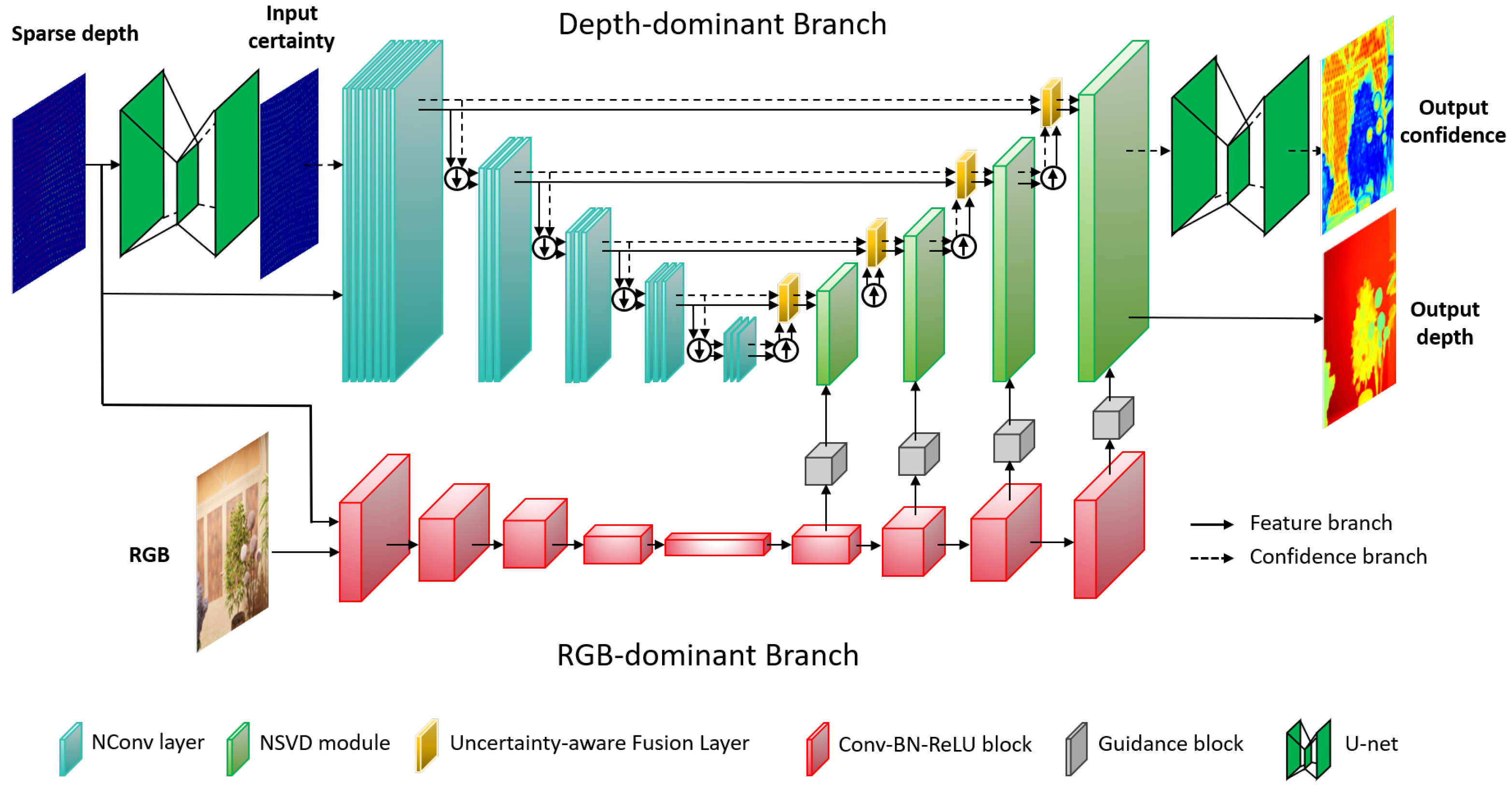
4. Network Architecture

In this section, we propose the normalized spatial-variant diffusion network (NSVDNet) for image-guided depth completion based on the NSVD module proposed in Section 3. As illustrated in Figure 2, the network is composed of the depth-dominant branch, which estimates the initial dense depth from the sparse sensor depth, and the RGB-dominant branch, which generates the semantic structural features. The two branches are fused in the hierarchical NSVD modules, where the initial dense depth is diffused with spatial-variant diffusion kernels constructed from RGB features. Details are provided as follows.

4.1. Depth-Dominant Branch

A hierarchical multi-scale architecture based on the U-Net [37] is adopted for the depth-dominant branch, which is illustrated at the top of Figure 2. First, the input confidence estimation network is adopted from [6], which uses sparse depth input to produce an estimate for the input confidence, indicating the reliability of the depth measurements, i.e., $\mathbf{S}$ in (2). The sparse depth and the estimated confidence are then fed into the encoder of the depth branch, which adopts the NConv layer from [38] for initial dense depth estimation. At the decoder, we use the proposed NSVD modules to refine depth at each scale, and the features from the encoder are fused with the decoder features via the uncertainty-aware feature fusion as follows.

4.2. Uncertainty-Aware Feature Fusion

To preserve details in the input features, skip connections are used to fuse the features at the corresponding scale. While direct concatenation will increase the feature channels, thus increasing the computational complexity in NSVConv layer, we instead fuse the features from the encoder and decoder via the uncertainty-aware feature fusion. Specifically, at each scale l, the decoder feature ${\mathbf{x}}_l^{dec}$ with corresponding ${\mathbf{s}}_l^{dec}$ and the encoder feature ${\mathbf{x}}_l^{enc}$ with corresponding ${\mathbf{s}}_l^{enc}$ at the same scale are fused based on the certainty, which generates the fused feature ${\mathbf{x}}_l^{fuse}$ as,

$$\begin{array}{c}\hfill {\mathbf{x}}_l^{fuse}=\frac{{\mathbf{s}}_l^{dec}⨀{\mathbf{x}}_l^{dec}+{\mathbf{s}}_l^{enc}⨀{\mathbf{x}}_l^{enc}}{{\mathbf{s}}_l^{dec}+{\mathbf{s}}_l^{enc}},\end{array}$$

(7)

and the output confidence is computed as

$$\begin{array}{c}\hfill {\mathbf{s}}_l^{fuse}=\frac{{\mathbf{s}}_l^{dec}⨀{\mathbf{s}}_l^{dec}+{\mathbf{s}}_l^{enc}⨀{\mathbf{s}}_l^{enc}}{{\mathbf{s}}_l^{dec}+{\mathbf{s}}_l^{enc}}.\end{array}$$

(8)

With (7) and (8), we define the uncertainty-aware feature fusion module, which integrates the encoder–decoder features as well as the corresponding certainty. In our work, the features are fused at four different scales, i.e., $l\in \{1,1/2,1/4,1/8\}$. The fused depth features and certainty measures are then fed into the NSVD modules for further refinement.

4.3. RGB-Dominant Branch

In the NSVD modules, while the inputs are generated from the fused depth features, the spatial-variant kernels are generated from the RGB-dominant branch at the bottom of Figure 2. The network adopts the encoder–decoder structure built upon residual networks [39] with ResNet34 as the encoder backbone to extract features from both RGB and sparse depth input. Specifically, the encoder and the decoder are composed of the Conv-BN-ReLU layers, where each layer is composed of the convolution, Batch-Normalization, and ReLU layer. The output of the decoder features is fed into the guidance block to generate kernels in the corresponding scales in the depth-dominant branch, where the guidance block is implemented using two layers of Conv-BN-ReLU. The spatial-variant kernels generated from the guidance block are used as the filter weight for diffusing the depth features and the corresponding certainty, i.e., $\mathbf{W}$ used in (5) and (6).

4.4. Hierarchical Normalized Spatial-Variant Diffusion

For efficient depth diffusion, the NSVD modules are applied hierarchically at the different scales in the decoder so that the spatial-variant diffusion operates at both the global region for overall scene depth accuracy and the local region for detail refinement. We adopt four NSVD modules for hierarchical calculation. For the modules at the smaller scales, i.e., scales of $1/8$ and $1/4$, the spatial-variant diffusion in NSVD covers a non-local region, which promotes global smoothness and overall scene depth accuracy. For the modules at the larger scales, i.e., $1/2$ scale and original scale, NSVD operates at a localized neighborhood, which refines the structural details. Meanwhile, the noise variance estimation network takes the output certainty from the last NSVD module as input to provide the final output depth certainty.

4.5. Loss Function

For the accurate prediction of the dense depth map, we train our network with the reconstruction loss function below supervised by the ground truth depth:

$$\begin{array}{cc}\hfill L_{recon}& ({\mathbf{x}}^{gt},{\mathbf{x}}^{pred},{\mathbf{s}}^{pred})=\hfill \\ \hfill & \frac{1}{\left|\mathcal{V}\right|}\sum _{v\in \mathcal{V}}[{\mathbf{s}}_v^{pred}{({\mathbf{x}}_v^{pred}-{\mathbf{x}}_v^{gt})}^2-log\left({\mathbf{s}}_v^{pred}\right)]\hfill \end{array}$$

(9)

where ${\mathbf{x}}^{gt}$ is the ground-truth depth, ${\mathbf{x}}^{pred}$ is the predicted dense depth, and ${\mathbf{s}}^{pred}$ is the output certainty measure. ${\mathbf{x}}_v$, $\mathcal{V}$, and $\left|\mathcal{V}\right|$ denote the depth values at pixel index v, the valid pixels of ${\mathbf{x}}^{gt}$, and the number of valid pixels, respectively. The first term in (9) is the data term weighted by the certainty measure, where high weights are assigned to more reliable measures. The second term is the regularization term for the certainty estimation, to avoid the trivial solution where ${\mathbf{s}}^{pred}$ goes all zero. Note that we do not maintain any supervision of the certainty because there is no ground truth; therefore, it is indirectly trained based on $L_{recon}$.

5. Experimental Results

In this section, we evaluate the depth completion performance of the proposed NSVDNet and demonstrate a comparison with existing algorithms, including sparse-to dense [14]; NCONV with RGB guidance using EncDec-Net [38]; CSPN [31]; and NLSPN [11]. We first provide a description of the implementation details in Section 5.1, where the network architecture details are provided in Table 1 and Table 2. Then, quantitative and qualitative comparisons to previous algorithms on indoor and outdoor datasets are presented and organized as follows.

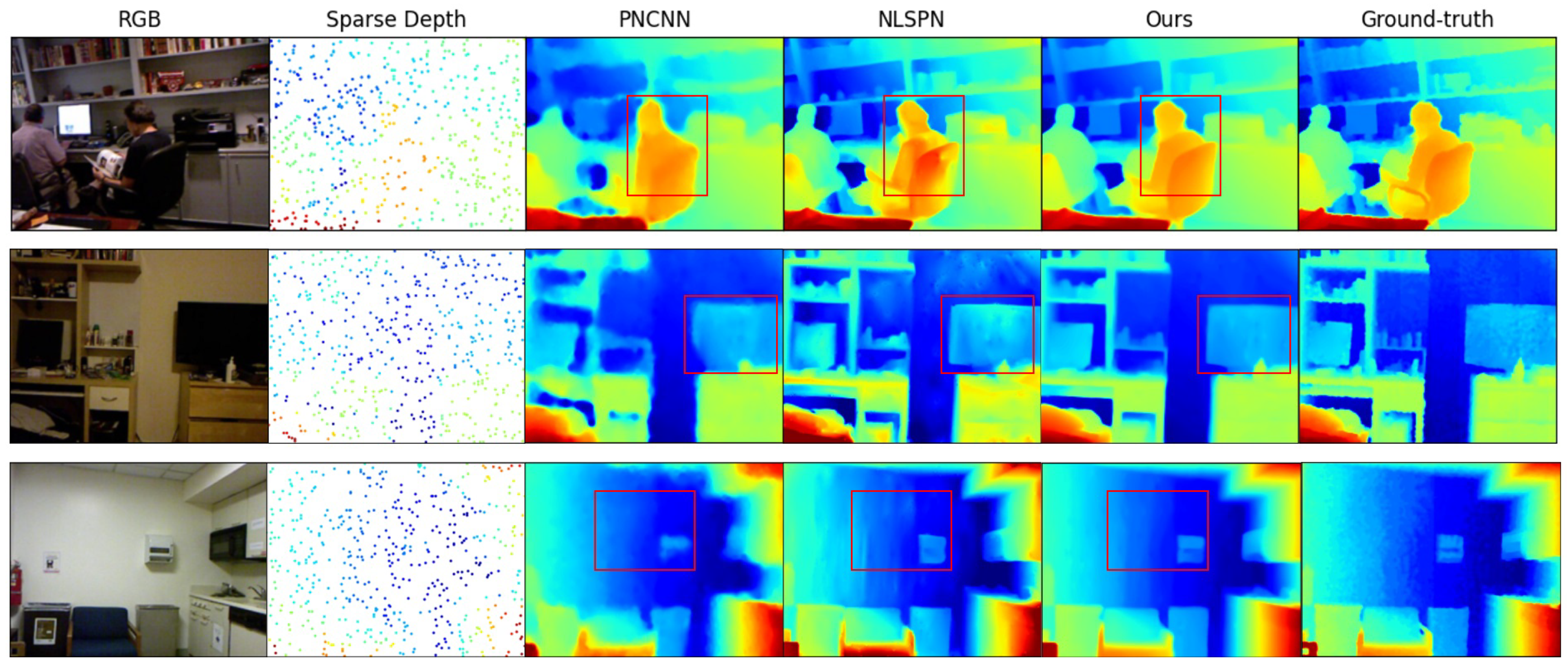
• In Section 5.2, we adopt the NYUv2 [12] and KITTI [20] datasets for evaluation in indoor and outdoor scenarios. The quantitative evaluation results using the two datasets are shown in Table 3 and Table 4, respectively, while the qualitative results further demonstrates the visual comparison using the NYUv2 dataset.
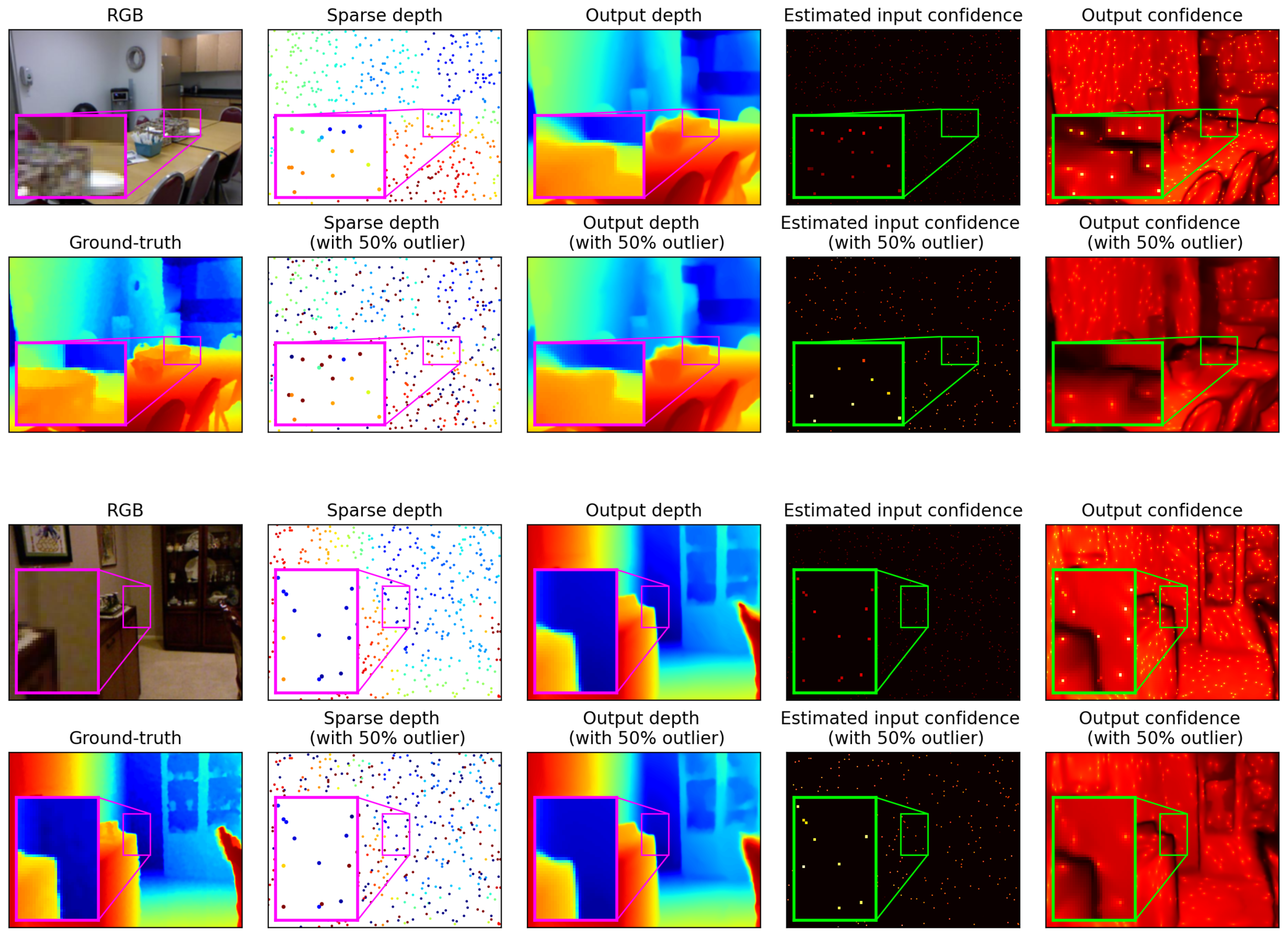
• In Section 5.3, we focus on the evaluation of robustness to input corruption in sparse depth, where we simulate corrupted sparse-depth using NYUv2 and show strong robustness of NSVDNet.
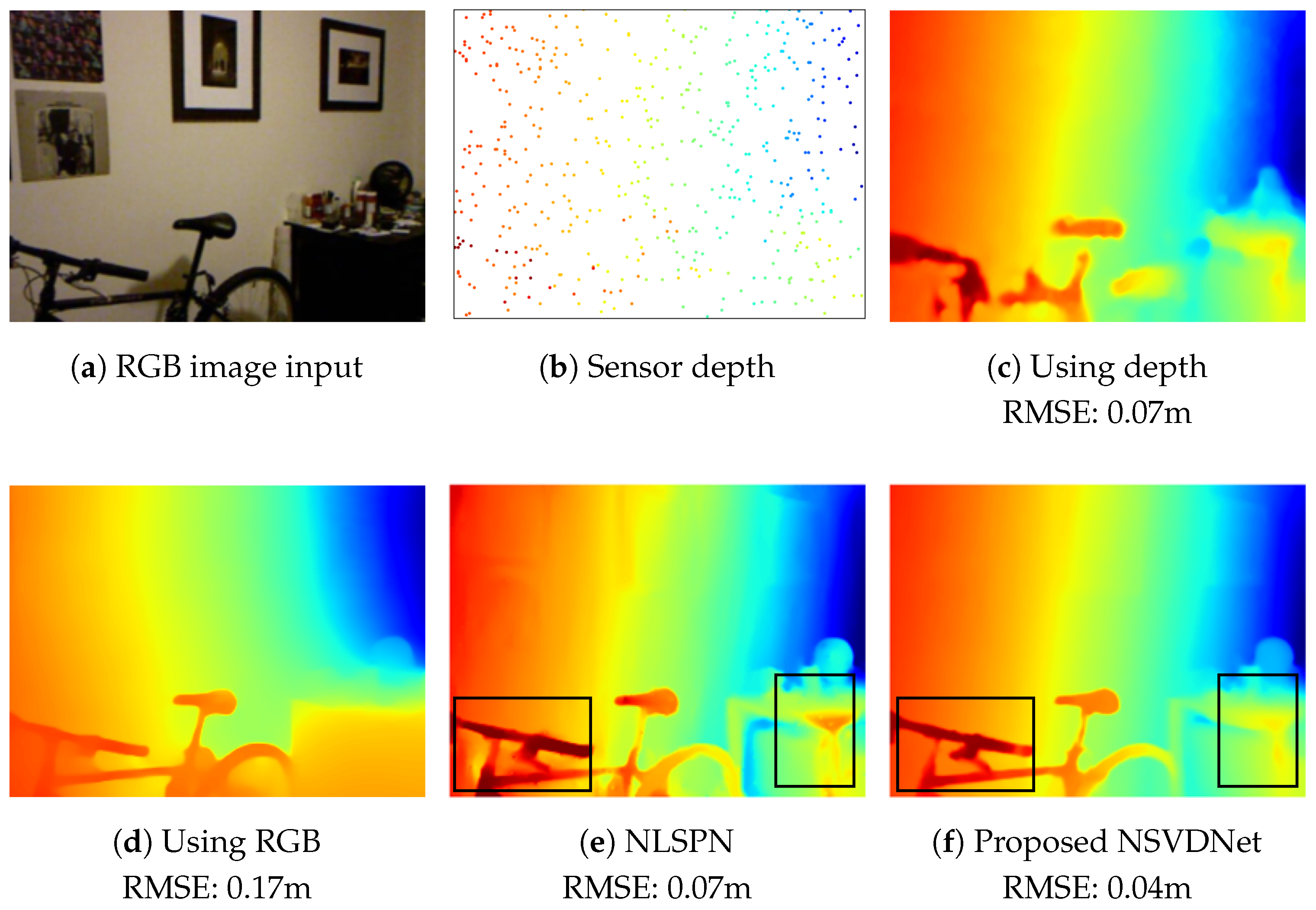
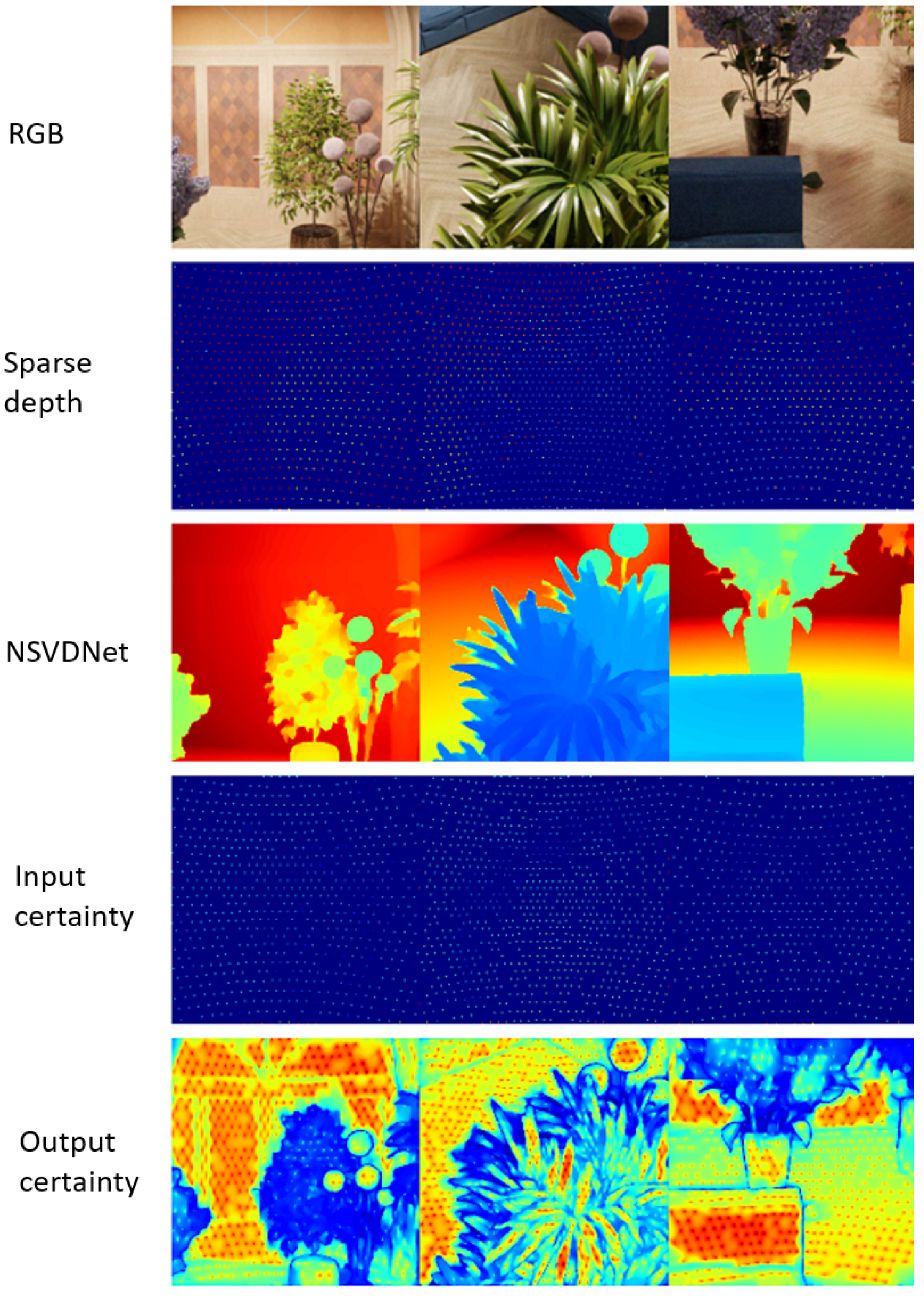
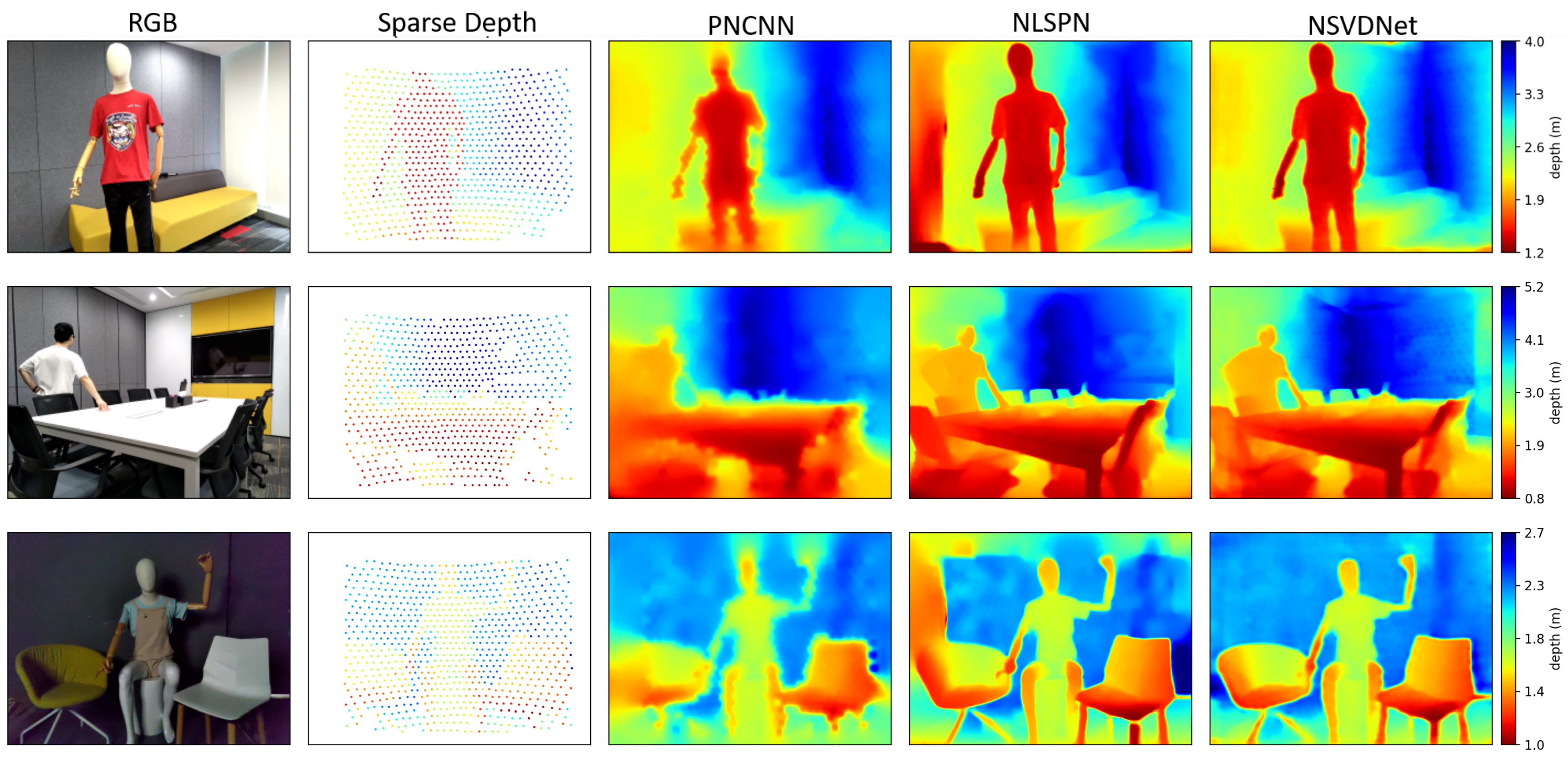
• In Section 5.3, we further test the generalization ability of NSVDNet to the new dataset via testing on the TetrasRGBD dataset [40] with the model trained on the NYUv2 noisy dataset. The visual results using simulated noise and the visual comparison with existing schemes using real sensor data are demonstrated, which validates that NSVDNet has a strong generalization ability to real usage scenarios.
• In Section 5.4, we present ablation studies to verify the effectiveness of each module in the NSVDNet.

5.1. Implementation Details

Training Details: We use the Adam optimizer with the initial learning rate set to ${10}^{-3}$ and decayed at epoch $[10,20,30,40]$ with decay rate $0.1$. The model is trained from scratch without a pretrained model for 50 epochs. We implement with PyTorch 1.10.1 [41] on 2 NVIDIA GeForce RTX 3090 GPUs.

Network Architecture: Details of the NSVDNet architecture are shown in Table 1 and Table 2, illustrating the depth-dominant branch and the RGB-dominant branch, respectively. Here, we use the input size of $256\times 256$ as the example, and input and output dimensions are shown in the table where H, W, and D denote the height, weight, and channel number of the input/output tensors, respectively.

As shown in Table 1, the depth-dominant branch takes the sparse depth as input and generates input certainty using UNet [6]; then, the sparse depth and input certainty are fed into the encoder, which is composed NConv layers [6] and MaxPool layers for downsampling. The decoder is composed of the proposed NSVD modules, uncertainty-aware fusion layers, and nearest-neighbor interpolation for upsampling, denoted as NSVD, Fusion, and NN interpolation, respectively. The number of iterations in NSVD modules is set to 10, which ensures result convergence. Along with the dense depth output, the decoder also outputs the confidence feature, which is fed into the output confidence estimator [6] for final confidence generation.

Table 1. Network Architecture for depth-dominant branch with input dimension $256\times 256$. For each module, the operators and the number of operators are specified. The input and output feature dimensions are specified, where H, W, and D refer to height, weight, and channel number of the tensors, respectively. The positions for input sparse depth and output dense depth/confidence are specified.

Module	Operator	# Operator	Input Dimension (H × W × D)	Output Dimension (H × W × D)
Input confidence estimator	UNet	1	256 × 256 × 1 (sparse depth)	256 × 256 × 1 (input certainty)
Encoder	NConv	7	256 × 256 × (1+1) (sparse depth + input certainty)	256 × 256 × 2
	MaxPool	1	256 × 256 × 2	128 × 128 × 2
	NConv	3	128 × 128 × 2	128 × 128 × 2
	MaxPool	1	128 × 128 × 2	64 × 64 × 2
	NConv	3	64 × 64 × 2	64 × 64 × 2
	MaxPool	1	64 × 64 × 2	32 × 32 × 2
	NConv	3	32 × 32 × 2	32 × 32 × 2
	MaxPool	1	32 × 32 × 2	16 × 16 × 2
	NConv	3	16 × 16 × 2	16 × 16 × 2
Decoder	NN interpolation	1	16 × 16 × 2	32 × 32 × 2
	Fusion	1	32 × 32 × (2 + 2)	32 × 32 × 2
	NSVD	1	32 × 32 × 2	32 × 32 × 2
	NN interpolation	1	32 × 32 × 2	64 × 64 × 2
	Fusion	1	64 × 64 × (2 + 2)	64 × 64 × 2
	NSVD	1	64 × 64 × 2	64 × 64 × 2
	NN interpolation	1	64 × 64 × 2	128 × 128 × 2
	Fusion	1	128 × 128 × (2 + 2)	128 × 128 × 2
	NSVD	1	128 × 128 × 2	128 × 128 × 2
	NN interpolation	1	128 × 128 × 2	256 × 256 × 2
	Fusion	1	256 × 256 × (2 + 2)	256 × 256 × 2
	NSVD	1	256 × 256 × 2	256 × 256 × (1 + 1) (output depth + confidence feature)
Output confidence estimator	UNet	1	256 × 256 × 1 (confidence feature)	256 × 256 × 1 (output confidence)

Table 1. Network Architecture for depth-dominant branch with input dimension $256\times 256$. For each module, the operators and the number of operators are specified. The input and output feature dimensions are specified, where H, W, and D refer to height, weight, and channel number of the tensors, respectively. The positions for input sparse depth and output dense depth/confidence are specified.

Module	Operator	# Operator	Input Dimension (H × W × D)	Output Dimension (H × W × D)
Input confidence estimator	UNet	1	256 × 256 × 1 (sparse depth)	256 × 256 × 1 (input certainty)
Encoder	NConv	7	256 × 256 × (1+1) (sparse depth + input certainty)	256 × 256 × 2
	MaxPool	1	256 × 256 × 2	128 × 128 × 2
	NConv	3	128 × 128 × 2	128 × 128 × 2
	MaxPool	1	128 × 128 × 2	64 × 64 × 2
	NConv	3	64 × 64 × 2	64 × 64 × 2
	MaxPool	1	64 × 64 × 2	32 × 32 × 2
	NConv	3	32 × 32 × 2	32 × 32 × 2
	MaxPool	1	32 × 32 × 2	16 × 16 × 2
	NConv	3	16 × 16 × 2	16 × 16 × 2
Decoder	NN interpolation	1	16 × 16 × 2	32 × 32 × 2
	Fusion	1	32 × 32 × (2 + 2)	32 × 32 × 2
	NSVD	1	32 × 32 × 2	32 × 32 × 2
	NN interpolation	1	32 × 32 × 2	64 × 64 × 2
	Fusion	1	64 × 64 × (2 + 2)	64 × 64 × 2
	NSVD	1	64 × 64 × 2	64 × 64 × 2
	NN interpolation	1	64 × 64 × 2	128 × 128 × 2
	Fusion	1	128 × 128 × (2 + 2)	128 × 128 × 2
	NSVD	1	128 × 128 × 2	128 × 128 × 2
	NN interpolation	1	128 × 128 × 2	256 × 256 × 2
	Fusion	1	256 × 256 × (2 + 2)	256 × 256 × 2
	NSVD	1	256 × 256 × 2	256 × 256 × (1 + 1) (output depth + confidence feature)
Output confidence estimator	UNet	1	256 × 256 × 1 (confidence feature)	256 × 256 × 1 (output confidence)

As shown in Table 2, we adopt ResNet34 [39] as our encoder–decoder baseline network for the RGB-dominant branch. To generate the spatial-variant kernels, the features from the decoder are fed into the guidance layers before fed into the NSVD modules, where the guidance layer is implemented using two layers of Conv-BN-ReLU. The number of output features from the guidance layers for spatial-variant kernels is set to 9 for a fair comparison to other affinity-based algorithms using $3\times 3$ local neighbors.

Table 2. Network Architecture for RGB-dominant Branch with input dimension $256\times 256$. For each module, the layer type is specified. The input and output feature dimensions are specified, where H, W, and D refer to height, weight, and channel number of the tensors, respectively. The positions for sparse depth and RGB input are specified, and the features generated by the guidance modules are fed into the NSVD modules in the depth-dominant branch.

Module	Layer	Input Dimension (H × W × D)	Output Dimension (H × W × D)
Encoder	Conv-BN-ReLU	256 × 256 × (1 + 3)	256 × 256 × 64
		(sparse depth + RGB image)
Encoder	ResNet34-layer1	256 × 256 × 64	256 × 256 × 64
Encoder	ResNet34-layer2	256 × 256 × 64	128 × 128 × 128
Encoder	ResNet34-layer3	128 × 128 × 128	64 × 64 × 256
Encoder	ResNet34-layer4	64 × 64 × 256	32 × 32 × 512
Encoder	Conv-BN-ReLU	32 × 32 × 512	16 × 16 × 512
Decoder	Convt-BN-ReLU	16 × 16 × 512	32 × 32 × 256
Guidance	Conv-BN-ReLU	32 × 32 × (256 + 512)	32 × 32 × 64
	Conv-BN-ReLU	32 × 32 × 64	32 × 32 × 9
Decoder	Convt-BN-ReLU	32 × 32 × (256 + 512)	64 × 64 × 128
Guidance	Conv-BN-ReLU	64 × 64 × (128 + 256)	64 × 64 × 64
	Conv-BN-ReLU	64 × 64 × 64	64 × 64 × 9
Decoder	Convt-BN-ReLU	64 × 64 × (128 + 256)	128 × 128 × 64
Guidance	Conv-BN-ReLU	128 × 128 × (64 + 128)	128 × 128 × 64
	Conv-BN-ReLU	128 × 128 × 64	128 × 128 × 9
Decoder	Convt-BN-ReLU	128 × 128 × (64 + 128)	256 × 256 × 64
Guidance	Conv-BN-ReLU	256 × 256 × (64 + 64)	256 × 256 × 64
	Conv-BN-ReLU	256 × 256 × 64	256 × 256 × 9

Table 2. Network Architecture for RGB-dominant Branch with input dimension $256\times 256$. For each module, the layer type is specified. The input and output feature dimensions are specified, where H, W, and D refer to height, weight, and channel number of the tensors, respectively. The positions for sparse depth and RGB input are specified, and the features generated by the guidance modules are fed into the NSVD modules in the depth-dominant branch.

Module	Layer	Input Dimension (H × W × D)	Output Dimension (H × W × D)
Encoder	Conv-BN-ReLU	256 × 256 × (1 + 3)	256 × 256 × 64
		(sparse depth + RGB image)
Encoder	ResNet34-layer1	256 × 256 × 64	256 × 256 × 64
Encoder	ResNet34-layer2	256 × 256 × 64	128 × 128 × 128
Encoder	ResNet34-layer3	128 × 128 × 128	64 × 64 × 256
Encoder	ResNet34-layer4	64 × 64 × 256	32 × 32 × 512
Encoder	Conv-BN-ReLU	32 × 32 × 512	16 × 16 × 512
Decoder	Convt-BN-ReLU	16 × 16 × 512	32 × 32 × 256
Guidance	Conv-BN-ReLU	32 × 32 × (256 + 512)	32 × 32 × 64
	Conv-BN-ReLU	32 × 32 × 64	32 × 32 × 9
Decoder	Convt-BN-ReLU	32 × 32 × (256 + 512)	64 × 64 × 128
Guidance	Conv-BN-ReLU	64 × 64 × (128 + 256)	64 × 64 × 64
	Conv-BN-ReLU	64 × 64 × 64	64 × 64 × 9
Decoder	Convt-BN-ReLU	64 × 64 × (128 + 256)	128 × 128 × 64
Guidance	Conv-BN-ReLU	128 × 128 × (64 + 128)	128 × 128 × 64
	Conv-BN-ReLU	128 × 128 × 64	128 × 128 × 9
Decoder	Convt-BN-ReLU	128 × 128 × (64 + 128)	256 × 256 × 64
Guidance	Conv-BN-ReLU	256 × 256 × (64 + 64)	256 × 256 × 64
	Conv-BN-ReLU	256 × 256 × 64	256 × 256 × 9

Evaluation Metrics: For quantitative evaluation, we adopted the commonly used metrics [11]:

• The Root Mean Squared Error (RMSE):
  $\sqrt{\frac{1}{\left|\nu \right|}{\sum }_{v\in \nu }{(d_v^{gt}-d_v^{pred})}^2}$;
• The Mean Absolute Error (MAE):
  $\frac{1}{\left|\nu \right|}{\sum }_{v\in \nu }|d_v^{gt}-d_v^{pred}|$;
• The Root Mean Squared Error of the inverse depth (iRMSE):
  $\sqrt{\frac{1}{\left|\nu \right|}{\sum }_{v\in \nu }{(\frac{1}{d_v^{gt}}-\frac{1}{d_v^{pred}})}^2}$;
• The Mean Absolute Error of the inverse depth (iMAE):
  $\frac{1}{\left|\nu \right|}{\sum }_{v\in \nu }|\frac{1}{d_v^{gt}}-\frac{1}{d_v^{pred}}|$;

Datasets: To demonstrate the performance in both indoor and outdoor scenarios, we adopt the NYUv2 [12] and KITTI [20] datasets for evaluation. Furthermore, the TetrasRGBD dataset [40] is used to evaluate the generalization ability of the proposed network to the unseen test dataset with simulated sensor noise.

5.2. Main Results

NYU Depth v2: The NYUv2 dataset contains video sequences from a variety of indoor scenes recorded by both the RGB and depth cameras from the Microsoft Kinect. Following [11], we use a subset of 45K images from the official training split as training data, and 654 official labeled images are used for evaluation. Every image is resized to $320\times 240$ and then center-cropped to $304\times 228$.

Similar to previous works [11], we randomly sampled 500 points from the ground truth depth as the sparse depth, which is combined with RGB image as the input of our network. Table 3 shows the quantitative result of our method on the NYUv2 dataset, and we can see that the proposed NSVDNet outperforms existing schemes, including sparse-to dense [14]; NCONV with RGB guidance using EncDec-Net [38]; CSPN [31]; and NLSPN [11].

In addition, we provide the number of network parameters of the competing methods in Table 3. The proposed method achieves the best performance with a reasonable amount of network parameters. We also provide the average running time (s) in Table 3, which is tested on one GeForce RTX 3090 GPU. As shown in Table 3, the most competitive method—NLSPN—consumes a higher runtime, while NSVDNet achieves higher accuracy at moderate complexity with a 43% runtime reduction. Therefore, NSVDNet outperforms competing methods with high efficiency, which is suitable for real-time applications.

Table 3. Quantitative evaluation of NYUv2 dataset compared with existing schemes, including Sparse2Dense, NCONV, CSPN, and NLSPN, respectively.

Method	Runtime	# Params.	RMSE	MAE	iRMSE	iMAE
	(s)	(M)	(m)	(m)	(1/m)	(1/m)
Sparse2dense	0.010	42.82	$0.2097$	$0.1346$	$0.0394$	$0.0230$
NCONV	0.003	0.670	0.1232	0.0491	0.0176	0.0067
CSPN	0.020	17.41	0.1183	0.0472	0.0183	0.0071
NLSPN	0.016	25.84	$0.0922$	$0.0348$	$0.0139$	$0.0051$
Proposed NSVDNet	0.009	29.14	0.0908	0.0338	0.0129	0.0045

Table 3. Quantitative evaluation of NYUv2 dataset compared with existing schemes, including Sparse2Dense, NCONV, CSPN, and NLSPN, respectively.

Method	Runtime	# Params.	RMSE	MAE	iRMSE	iMAE
	(s)	(M)	(m)	(m)	(1/m)	(1/m)
Sparse2dense	0.010	42.82	$0.2097$	$0.1346$	$0.0394$	$0.0230$
NCONV	0.003	0.670	0.1232	0.0491	0.0176	0.0067
CSPN	0.020	17.41	0.1183	0.0472	0.0183	0.0071
NLSPN	0.016	25.84	$0.0922$	$0.0348$	$0.0139$	$0.0051$
Proposed NSVDNet	0.009	29.14	0.0908	0.0338	0.0129	0.0045

To demonstrate visual comparison, in Figure 3, we show our depth completion results tested with the NYUv2 dataset with a qualitative comparison to the depth-only PNCNN, and the state-of-the-art NLSPN. We can see that with only the depth input, the result of PNCNN has blurry edges and the object shapes are not preserved. Meanwhile, with RGB guidance, NLSPN and the proposed NSVDNet provide much sharper and more complete depth details. However, without certainty guidance, NLSPN introduces extra textures, e.g., the back of the chair contains a bumpy surface in the first row of Figure 3. This is because the initial depth and affinity matrix are implicitly learnt lacking interpretability. On the other hand, with the inherent diffusion model in the network design, the proposed NSVDNet gives sharp results without extra textures from the RGB features. This is consistent with the metric values in Table 3.

KITTI Depth Completion Dataset: The KITTI dataset is an outdoor dataset for autonomous driving, which contains 85,000 color images and corresponding dense annotated depth maps and sparse raw LiDAR scans for training, 6000 for validation, and 1000 for testing. One thousand color images and corresponding sparse depth maps with unpublished depth maps are selected as the benchmark for algorithm evaluation. For training, we crop the first 100 rows of color and depth images (which have no corresponding ground truth depth) and then randomly crop color and depth images to $1216\times 240$.

Table 4 shows the quantitative result of our method on the KITTI DC dataset, and we can see that the proposed approach outperforms existing schemes, including sparse-to dense [14], NCONV with RGB guidance [38], CSPN [31], PENet [33], and NLSPN [11]. Note that the performance enhancement is less obvious because the input depth noise level is small, and the advantage of noise robustness in NSVDNet is not fully exhibited. Nevertheless, NSVDNet achieves competing results due to the hierarchical spatially adaptive filtering.

Table 4. Quantitative evaluation on KITTI DC dataset compared with existing schemes, including Sparse2Dense, NCONV, CSPN, PENet, and NLSPN.

Method	RMSE	MAE	iRMSE	iMAE
	(mm)	(mm)	(1/km)	(1/km)
Sparse2dense	1299.851	350.326	4.073	1.576
NCONV	1009.258	238.692	2.917	1.007
CSPN	1019.64	279.46	2.932	1.151
PENet	757.197	209.001	2.222	0.923
NLSPN	741.685	199.594	1.994	0.845
NSVDNet	739.645	196.451	2.032	0.832

Table 4. Quantitative evaluation on KITTI DC dataset compared with existing schemes, including Sparse2Dense, NCONV, CSPN, PENet, and NLSPN.

Method	RMSE	MAE	iRMSE	iMAE
	(mm)	(mm)	(1/km)	(1/km)
Sparse2dense	1299.851	350.326	4.073	1.576
NCONV	1009.258	238.692	2.917	1.007
CSPN	1019.64	279.46	2.932	1.151
PENet	757.197	209.001	2.222	0.923
NLSPN	741.685	199.594	1.994	0.845
NSVDNet	739.645	196.451	2.032	0.832

5.3. Data with Corruption

NYU Depth v2 with Simulated Corruption: In real-world scenarios, the captured depth is highly likely to be corrupted by noise. To demonstrate the robustness of our algorithm to noisy depth input, we simulate the corrupted sparse-depth using the NYUv2 depth dataset. Specially, we randomly set $50\%$ of the outliers in the sparse depth, including $25\%$ of the valid pixels to be 10 m, which is the maximum depth value, and $25\%$ to be 0 m, which is the minimum depth value. The network is retrained on the NYUv2 dataset with simulated noise. The visual results are provided in Figure 4, comparing the cases of adding and not adding outliers to the sparse input.

As shown in Figure 4, the output depth of NSVDNet is not obviously affected by the input outliers, demonstrating good overall smoothness and detail preservation. This is due to the input certainty estimation that distinguishes the outliers from the accurate pixels and excludes the outliers from propagating to neighboring pixels. For better demonstration, we provide a zoom-in version of a selected region of each scene. All depth-related images are colored with the ‘jetr’ color map. All of the certainty maps are colored with the ‘hot’ color map. The black pixels indicate a low certainty value, and the yellow pixels indicate a high certainty value. All of the outliers are set to almost-zero values in the estimated input certainty, which explains why NSVDNet is able to suppress the noise. Moreover, the output certainty map provides the confidence measurement for the depth estimation, where we can see the outliers obviously decrease the confidence for known pixels, providing an accurate output reliability map.

Generalization Evaluation on TetrasRGBD: To test the generalization ability of NSVDNet on the new dataset, we use the model trained on NYUv2 noisy dataset and test with the new dataset called TetrasRGBD [40]. TetrasRGBD contains 2.3k pairs of testing data from mixed sources. All the data are collected in indoor scenarios, and the synthetic dataset is generated with ground-truth 3D geometry.

To demonstrate the robustness to noisy depth measurement, we adopt the TetrasRGBD dataset augmented with outliers in sparse depth input. As shown in Figure 5, 20% of the pixels in the sparse depth are corrupted by outliers. The proposed NSVDNet generalizes well to the unseen test dataset, showing strong robustness to the outliers and high depth estimation accuracy. This is due to the use of interpretable uncertainty-aware diffusion that limits the solution space of the network and avoids overfitting to the training data. To visualize how NSVD rivals the noisy input, Figure 5 shows the estimated certainty map for the input, indicating depth measurement reliability. When used in the NSVD module, the certainty map prevents outlier information from propagating to the neighboring pixels. Further, the output certainty provides the reliability of the network output depth, where we can see the known depth pixels show higher values, while the regions with fine details show lower values, which are typical with lower accuracy.

To further demonstrate the generalization to real-world scenarios, we use the real data captured by mobile devices provided in the TetrasRGBD dataset [40] for testing, where the input depth suffers from large sensor noise. We again use the pre-trained model trained on the NYUv2 noisy dataset, and the results are shown in Figure 6. By comparison with competitive methods, including PNCNN [38] and NLSPN [11], the proposed NSVDNet shows more accurate global depth estimation with sharp structural details. In sum, the evaluation with real sensor data illustrates the strong generalization ability of NSVDNet, indicating the potential to apply NSVDNet in practice.

5.4. Ablation Study

In the ablation study, we regard the PNCNN network [6] as a simplified variant of the proposed NSVDNet, which replaces the NSVD module with the NConv module without spatial-varying filters and hierarchical implementation. With PNCNN as the baseline model, we then show a comparison among different variants in

Table 5. Ablation study using TetrasRGBD dataset. With PNCNN as the baseline model, we compare multi-scale NSVD (MS-NSVD) used in NSVDNet with simplified variant single-scale NSVD (OS-NSVD), where MS-NSVD outperforms OS-NSVD due to enhanced global smoothness. Additionally, we compare feature-fusion (FF) used in NSVDNet with its variant feature-concatenation (FC), where FF outperforms FC due to the utilization of input uncertainty.

Metrics	PNCNN + FC + OS-NSVD	PNCNN + FF + OS-NSVD	PNCNN + FF + MS-NSVD
MAE(m)	0.0706	0.0677	0.0615
RMSE(m)	0.2704	0.2619	0.2447
iMAE(1/m)	0.0064	0.0061	0.0056
iRMSE(1/m)	0.0229	0.0221	0.0209

that validates the importance of the designed modules. First, we compare the multi-scale deployment and single-scale deployment of NSVD, which are referred to as MS-NSVD and OS-NSVD, respectively. By comparing PNCNN+FF+MS-NSVD and PNCNN+FF+OS-NSVD in Table 5, we can see that MS-NSVD greatly improves compared to OS-NSVD due its enhanced global smoothness.

Next, we compare the uncertainty-aware feature-fusion with feature-concatenation used in the dept decoder, which are referred to as FF and FC, respectively. By comparing PNCNN+FC+OS-NSVD and PNCNN+FF+OS-NSVD in Table 5, we can see that a simple concatenation without considering depth feature certainty can degrade the final prediction due to the inclusion of low-confident features in the decoder.

6. Conclusions

In this work, we propose a hierarchical normalized spatial-variant diffusion network for image-guided depth completion. The network is designed to incorporate the anisotropic diffusion model, where the diffusion is deployed via the proposed normalized spatial-variant diffusion (NSVD) module. NSVD diffuses the input depth feature and corresponding confidence with the semantic structural guidance extracted from the RGB image. Moreover, the hierarchical deployment of NSVD modules is adopted to ensure both global smoothness and local details. Extensive experimental results demonstrate that the proposed NSVDNet outperforms the existing methods at providing more accurate depth completion and sharper visually salient features. Ablation studies validate the effectiveness of the proposed hierarchical NSVDNet at enhancing the robustness to noisy pixels in the sensor depth input.

Despite the improvements introduced by the proposed network, focusing on interpretable depth diffusion design with noise robustness, several limitations still remain requiring further investigation. Instead of utilizing localized spatial filtering in the depth diffusion, future work could develop more powerful spatial filtering techniques to exploit adaptive neighborhood with non-local filtering kernels. In this way, a longer-range context would be involved in the diffusion with more accurate global smoothness and faster convergence. More importantly, the non-local filtering would benefit from the case where more severe noise corruption were involved with non-uniform sparsity.

Another crucial aspect that needs to be considered in future work is the time-domain consistency in depth video completion, which is required in various applications such as 3D scene reconstruction and SLAM. This aspect necessitates depth completion to enforce coherence between consecutive frames. Furthermore, the redundancy in temporal sequence can be utilized to reduce the computational complexity by re-using the features from neighboring frames. Toward this end, we plan to explore the spatial-temporal depth video completion algorithm to enhance algorithm efficiency and temporal consistency, which should be of great importance to real-time 3D vision applications.

References

1. Dong, X.; Garratt, M.A.; Anavatti, S.G.; Abbass, H.A. Towards real-time monocular depth estimation for robotics: A survey. IEEE Trans. Intell. Transp. Syst. 2022, 23, 16940–16961. [Google Scholar] [CrossRef]
2. Fu, C.; Mertz, C.; Dolan, J.M. Lidar and monocular camera fusion: On-road depth completion for autonomous driving. In Proceedings of the 2019 IEEE Intelligent Transportation Systems Conference (ITSC), Auckland, New Zealand, 27–30 October 2019; IEEE: Piscataway, NJ, USA, 2019; pp. 273–278. [Google Scholar]
3. Kahn, S. Reducing the gap between Augmented Reality and 3D modeling with real-time depth imaging. Virtual Real. 2013, 17, 111–123. [Google Scholar] [CrossRef]
4. Nowak, M.K. WeaveNet: Solution for Variable Input Sparsity Depth Completion. Electronics 2022, 11, 2222. [Google Scholar] [CrossRef]
5. El-Yabroudi, M.Z.; Abdel-Qader, I.; Bazuin, B.J.; Abudayyeh, O.; Chabaan, R.C. Guided Depth Completion with Instance Segmentation Fusion in Autonomous Driving Applications. Sensors 2022, 22, 9578. [Google Scholar] [CrossRef] [PubMed]
6. Eldesokey, A.; Felsberg, M.; Holmquist, K.; Persson, M. Uncertainty-aware cnns for depth completion: Uncertainty from beginning to end. In Proceedings of the IEEE/CVF Conference on Computer Vision and Pattern Recognition, Seattle, WA, USA, 13–19 June 2020; pp. 12014–12023. [Google Scholar]
7. Ranftl, R.; Lasinger, K.; Hafner, D.; Schindler, K.; Koltun, V. Towards robust monocular depth estimation: Mixing datasets for zero-shot cross-dataset transfer. IEEE Trans. Pattern Anal. Mach. Intell. 2020, 44, 1623–1637. [Google Scholar] [CrossRef] [PubMed]
8. Fu, H.; Gong, M.; Wang, C.; Batmanghelich, K.; Tao, D. Deep ordinal regression network for monocular depth estimation. In Proceedings of the IEEE/CVF Conference on Computer Vision and Pattern Recognition, Salt Lake City, UT, USA, 18–23 June 2018; pp. 2002–2011. [Google Scholar]
9. You, Y.; Wang, Y.; Chao, W.L.; Garg, D.; Pleiss, G.; Hariharan, B.; Campbell, M.; Weinberger, K.Q. Pseudo-LiDAR++: Accurate Depth for 3D Object Detection in Autonomous Driving. In Proceedings of the International Conference on Learning Representations (ICLR), Addis Ababa, Ethiopia, 30 April 2020. [Google Scholar]
10. Li, Y.; Yu, A.W.; Meng, T.; Caine, B.; Ngiam, J.; Peng, D.; Shen, J.; Lu, Y.; Zhou, D.; Le, Q.V.; et al. Deepfusion: Lidar-camera deep fusion for multi-modal 3d object detection. In Proceedings of the IEEE/CVF Conference on Computer Vision and Pattern Recognition, New Orleans, LA, USA, 18–24 June 2022; pp. 17182–17191. [Google Scholar]
11. Park, J.; Joo, K.; Hu, Z.; Liu, C.K.; So Kweon, I. Non-local spatial propagation network for depth completion. In Proceedings of the European Conference on Computer Vision, Glasgow, UK, 23–28 August 2020; Springer: Berlin/Heidelberg, Germany, 2020; pp. 120–136. [Google Scholar]
12. Silberman, N.; Hoiem, D.; Kohli, P.; Fergus, R. Indoor segmentation and support inference from rgbd images. In Proceedings of the European Conference on Computer Vision, Florence, Italy, 7–13 October 2012; Springer: Berlin/Heidelberg, Germany, 2012; pp. 746–760. [Google Scholar]
13. Ren, W.; Jin, N.; OuYang, L. Phase Space Graph Convolutional Network for Chaotic Time Series Learning. IEEE Trans. Ind. Inform. 2024, 20, 7576–7584. [Google Scholar] [CrossRef]
14. Ma, F.; Karaman, S. Sparse-to-dense: Depth prediction from sparse depth samples and a single image. In Proceedings of the 2018 IEEE International Conference on Robotics and Automation (ICRA), Brisbane, Australia, 21–25 May 2018; IEEE: Piscataway, NJ, USA, 2018; pp. 4796–4803. [Google Scholar]
15. Zhao, S.; Gong, M.; Fu, H.; Tao, D. Adaptive context-aware multi-modal network for depth completion. IEEE Trans. Image Process. 2021, 30, 5264–5276. [Google Scholar] [CrossRef] [PubMed]
16. Chang, A.; Dai, A.; Funkhouser, T.; Halber, M.; Niebner, M.; Savva, M.; Song, S.; Zeng, A.; Zhang, Y. Matterport3D: Learning from RGB-D Data in Indoor Environments. In Proceedings of the 2017 International Conference on 3D Vision (3DV), Qingdao, China, 10–12 October 2017; pp. 667–676. [Google Scholar]
17. Zeng, J.; Tong, Y.; Huang, Y.; Yan, Q.; Sun, W.; Chen, J.; Wang, Y. Deep surface normal estimation with hierarchical RGB-D fusion. In Proceedings of the IEEE/CVF Conference on Computer Vision and Pattern Recognition, Long Beach, CA, USA, 15–20 June 2019; pp. 6153–6162. [Google Scholar]
18. Shlezinger, N.; Whang, J.; Eldar, Y.C.; Dimakis, A.G. Model-based deep learning. Proc. IEEE 2023, 111, 465–499. [Google Scholar] [CrossRef]
19. Zeng, J.; Pang, J.; Sun, W.; Cheung, G. Deep graph Laplacian regularization for robust denoising of real images. In Proceedings of the IEEE/CVF Conference on Computer Vision and Pattern Recognition Workshops, Long Beach, CA, USA, 16–17 June 2019. [Google Scholar]
20. Uhrig, J.; Schneider, N.; Schneider, L.; Franke, U.; Brox, T.; Geiger, A. Sparsity invariant CNNs. In Proceedings of the 2017 International Conference on 3D Vision (3DV), Qingdao, China, 10–12 October 2017; IEEE: Piscataway, NJ, USA, 2017; pp. 11–20. [Google Scholar]
21. Ferstl, D.; Reinbacher, C.; Ranftl, R.; Rüther, M.; Bischof, H. Image guided depth upsampling using anisotropic total generalized variation. In Proceedings of the IEEE International Conference on Computer Vision, Sydney, Australia, 1–8 December 2013; pp. 993–1000. [Google Scholar]
22. Herrera, D.; Kannala, J.; Ladický, L.U.; Heikkilä, J. Depth map inpainting under a second-order smoothness prior. In Proceedings of the Scandinavian Conference on Image Analysis, Espoo, Finland, 17–20 June 2013; Springer: Berlin/Heidelberg, Germany, 2013; pp. 555–566. [Google Scholar]
23. Schneider, N.; Schneider, L.; Pinggera, P.; Franke, U.; Pollefeys, M.; Stiller, C. Semantically guided depth upsampling. In Proceedings of the German Conference on Pattern Recognition, Hannover, Germany, 12–15 September 2016; Springer: Berlin/Heidelberg, Germany, 2016; pp. 37–48. [Google Scholar]
24. Huang, Z.; Fan, J.; Cheng, S.; Yi, S.; Wang, X.; Li, H. Hms-net: Hierarchical multi-scale sparsity-invariant network for sparse depth completion. IEEE Trans. Image Process. 2019, 29, 3429–3441. [Google Scholar] [CrossRef] [PubMed]
25. Liu, L.; Song, X.; Sun, J.; Lyu, X.; Li, L.; Liu, Y.; Zhang, L. MFF-Net: Towards Efficient Monocular Depth Completion With Multi-Modal Feature Fusion. IEEE Robot. Autom. Lett. 2023, 8, 920–927. [Google Scholar] [CrossRef]
26. Zhang, Y.; Guo, X.; Poggi, M.; Zhu, Z.; Huang, G.; Mattoccia, S. CompletionFormer: Depth completion with convolutions and vision transformers. In Proceedings of the IEEE/CVF Conference on Computer Vision and Pattern Recognition, Vancouver, BC, Canada, 17–24 June 2023; pp. 18527–18536. [Google Scholar]
27. Zhou, W.; Yan, X.; Liao, Y.; Lin, Y.; Huang, J.; Zhao, G.; Cui, S.; Li, Z. BEV@ DC: Bird’s-Eye View Assisted Training for Depth Completion. In Proceedings of the IEEE/CVF Conference on Computer Vision and Pattern Recognition, Vancouver, BC, Canada, 17–24 June 2023; pp. 9233–9242. [Google Scholar]
28. Qiu, J.; Cui, Z.; Zhang, Y.; Zhang, X.; Liu, S.; Zeng, B.; Pollefeys, M. Deeplidar: Deep surface normal guided depth prediction for outdoor scene from sparse lidar data and single color image. In Proceedings of the IEEE/CVF Conference on Computer Vision and Pattern Recognition, Long Beach, CA, USA, 15–20 June 2019; pp. 3313–3322. [Google Scholar]
29. Chen, Y.; Yang, B.; Liang, M.; Urtasun, R. Learning joint 2d-3d representations for depth completion. In Proceedings of the IEEE/CVF International Conference on Computer Vision, Seoul, Republic of Korea, 27 October–2 November 2019; pp. 10023–10032. [Google Scholar]
30. Liu, S.; De Mello, S.; Gu, J.; Zhong, G.; Yang, M.H.; Kautz, J. Learning affinity via spatial propagation networks. Adv. Neural Inf. Process. Syst. 2017, 30, 1–11. [Google Scholar]
31. Cheng, X.; Wang, P.; Yang, R. Depth estimation via affinity learned with convolutional spatial propagation network. In Proceedings of the European Conference on Computer Vision (ECCV), Munich, Germany, 8–14 September 2018; pp. 103–119. [Google Scholar]
32. Cheng, X.; Wang, P.; Guan, C.; Yang, R. Cspn++: Learning context and resource aware convolutional spatial propagation networks for depth completion. In Proceedings of the AAAI Conference on Artificial Intelligence, Hilton, NY, USA, 7–12 February 2020; Volume 34, pp. 10615–10622. [Google Scholar]
33. Hu, M.; Wang, S.; Li, B.; Ning, S.; Fan, L.; Gong, X. PENet: Towards Precise and Efficient Image Guided Depth Completion. In Proceedings of the IEEE International Conference on Robotics and Automation (ICRA), Xi’an, China, 30 May–5 June 2021. [Google Scholar]
34. Knutsson, H.; Westin, C.F. Normalized and differential convolution. In Proceedings of the IEEE Conference on Computer Vision and Pattern Recognition, New York, NY, USA, 15–17 June 1993; IEEE: Piscataway, NJ, USA, 1993; pp. 515–523. [Google Scholar]
35. Milanfar, P. A tour of modern image filtering: New insights and methods, both practical and theoretical. IEEE Signal Process. Mag. 2012, 30, 106–128. [Google Scholar] [CrossRef]
36. Perona, P.; Malik, J. Scale-space and edge detection using anisotropic diffusion. IEEE Trans. Pattern Anal. Mach. Intell. 1990, 12, 629–639. [Google Scholar] [CrossRef]
37. Ronneberger, O.; Fischer, P.; Brox, T. U-net: Convolutional networks for biomedical image segmentation. In Proceedings of the International Conference on Medical Image Computing and Computer-Assisted Intervention, Munich, Germany, 5–9 October 2015; Springer: Berlin/Heidelberg, Germany, 2015; pp. 234–241. [Google Scholar]
38. Eldesokey, A.; Felsberg, M.; Khan, F.S. Confidence propagation through cnns for guided sparse depth regression. IEEE Trans. Pattern Anal. Mach. Intell. 2019, 42, 2423–2436. [Google Scholar] [CrossRef] [PubMed]
39. He, K.; Zhang, X.; Ren, S.; Sun, J. Deep residual learning for image recognition. In Proceedings of the IEEE Conference on Computer Vision and Pattern Recognition, Las Vegas, NV, USA, 27–30 June 2016; pp. 770–778. [Google Scholar]
40. Sun, W.; Zhu, Q.; Li, C.; Feng, R.; Zhou, S.; Jiang, J.; Yang, Q.; Loy, C.C.; Gu, J.; Hou, D.; et al. Mipi 2022 challenge on rgb+ tof depth completion: Dataset and report. In Proceedings of the European Conference on Computer Vision, Tel Aviv, Israel, 23–27 October 2022; Springer: Berlin/Heidelberg, Germany, 2022; pp. 3–20. [Google Scholar]
41. Paszke, A.; Gross, S.; Chintala, S.; Chanan, G.; Yang, E.; DeVito, Z.; Lin, Z.; Desmaison, A.; Antiga, L.; Lerer, A. Automatic Differentiation in Pytorch. In Proceedings of the 31st Conference on Neural Information Processing Systems (NIPS 2017), Long Beach, CA, USA, 4–9 December 2017. [Google Scholar]
Figure 2. An overview of NSVDNet architecture to predict a dense depth from a disturbed sparse depth with RGB guidance. NSVDNet is composed of the depth-dominant branch, which estimates the initial dense depth from the sparse sensor depth, and the RGB-dominant branch, which generates the semantic structural features. The two branches are fused in the hierarchical NSVD modules, where the initial dense depth is diffused with spatial-variant diffusion kernels constructed from RGB features.
Electronics 13 02418 g002
Figure 3. Depth completion with different algorithms, tested on NYUv2 dataset. As highlighted in the red rectangles, the proposed NSVDNet achieves more accurate depth completion results with detail preservation and noise robustness.
Electronics 13 02418 g003
Figure 4. Comparison of depth completion with original sparse depth and noisy sparse depth with 50% outliers, tested on NYUv2 dataset. The comparison between results with original and noisy inputs demonstrates the robustness to input corruption for the proposed method. The selected patches are enlarged in the colored rectangles.
Electronics 13 02418 g004
Figure 5. Generalization ability evaluation tests on TetrasRGBD dataset with outliers. The certainty maps explain the robustness of NSVDNet to input corruptions.
Electronics 13 02418 g005
Figure 6. Generalization ability evaluation tests on TetrasRGBD dataset with real sensor data, where the proposed NSVDNet generates more accurate depth estimation than competitive methods, including PNCNN [38] and NLSPN [11].
Electronics 13 02418 g006