A Deep Learning Approach for Trajectory Control of Tilt-Rotor UAV

Abstract

This paper investigates the development of a deep learning-based flight control model for a tilt-rotor unmanned aerial vehicle, focusing on altitude, speed, and roll hold systems. Training data is gathered from the X-Plane flight simulator, employing a proportional–integral–derivative controller to enhance flight dynamics and data quality. The model architecture, implemented within the TensorFlow framework, undergoes iterative tuning for optimal performance. Testing involved two scenarios: wind-free conditions and wind disturbances. In wind-free conditions, the model demonstrated excellent tracking performance, closely tracking the desired altitude. The model’s robustness is further evaluated by introducing wind disturbances. Interestingly, these disturbances do not significantly impact the model performance. This research has demonstrated data-driven flight control in a tilt-rotor unmanned aerial vehicle, offering improved adaptability and robustness compared to traditional methods. Future work may explore further flight modes, environmental complexities, and the utilization of real test flight data to enhance the model generalizability.

1. Introduction

Tilt-rotor aircraft, considered unconventional configurations, combine the capabilities of both helicopters and fixed-wing aircraft. This unique design allows them to perform maneuvers traditionally associated with both types of aircraft. Consequently, tilt-rotor craft can perform vertical takeoff and landing (VTOL) within confined spaces while also exhibiting the extended range and endurance characteristics of fixed-wing aircraft during forward flight. However, the change in configuration throughout operation, achieved through tilting the rotors, introduces significant complexities in terms of dynamic response. Notably, the transition phase between helicopter and fixed-wing modes undergoes drastic changes in dynamic behavior, requiring specific considerations for handling and control.

In designing the flight controller of a tilt-rotor aircraft, the dynamic behavior during the transition phase must be anticipated and specifically treated. This is necessary to obtain a good-closed response during this critical maneuver. The potential of rotorcraft, especially tilt-rotor UAVs, has attracted institutions to develop this type of UAV [1,2]. The design and development of control systems for multi-rotor aircraft using different techniques are elaborated in many works, for example, in [3,4]. Some control techniques that have been used in recent tilt-rotor control development are described in [5], giving an insight into the challenges in the tilt-rotor flight control research area. An adaptive model inversion control approach is explored and implemented in [6] for developing a tilt-rotor flight control system. While, in [7], the non-linear Active Disturbance Rejection Control and Sliding Mode Control (SMC) methods are exploited for providing control of tilt-rotor aircraft in the transition flight phase. A robust (H-inf) linear control approach is proposed in [8] for constructing a tilt-rotor flight control system. This approach bases its control parameter computation on a set of linear systems, each of which represents a different flight phase of the aircraft, including the transition phase.

A scheduled control system for a conceptual tilt-rotor aircraft is developed in [9] by using two different controllers for providing body-axis horizontal and normal velocity commands. The handling of the quality criteria is also considered in this work. Flight control development for a quad-tilt-rotor UAV is discussed in [10], where the modeling and control law design are arranged in a geometric setting to obtain an intrinsic control law, providing stability and tracking capability. While, in reference [11], a control system for a hybrid UAV is discussed in which the controller is developed by implementing a control allocation scheme. The controller is constructed based on a linear approach and aims to tackle actuator saturation and disturbance problems. A robust reconfigurable control that can anticipate actuator failure is developed and implemented for a hybrid tilt-rotor system [12]. A switching controller strategy is employed to provide changes in controller parameters for some predefined failures. Research conducted in [13] presents works in developing a control allocation strategy for a tilt-rotor system, along with its implementation and flight test for evaluating the developed control scheme performance.

The multifaceted challenges associated with tilt-rotor aircraft development have driven continuous research efforts in the realm of control methodologies and strategies aimed at achieving desired performance outcomes. Data-driven learning techniques, fueled by rapid advancements in computational power, have emerged as a prominent approach within this diverse landscape. These learning-based methods offer compelling capabilities for enhancing controller performance through the provision of parameter adjustment and adaptation mechanisms. Ref. [14] presents insightful discussions on the application of data-learning methods across various domains, effectively demonstrating their potential for addressing diverse engineering challenges. Furthermore, reference [15] elaborates on the implementation of a neural network scheme utilizing a data-driven learning mechanism for computing controller parameters in the context of aircraft flight control systems. Notably, reference [16] delves into the implementation of this learning-based technique for tilt-rotor systems, highlighting its potential for achieving in-flight control parameter adaptation.

The application of neural network schemes in the context of VTOL control has been explored in numerous research endeavors. Notably, ref. [17] elaborates on the implementation of a neural network scheme for adapting controller parameters within a PID framework. Moreover, ref. [18] investigates the utilization of a neural network-based ADRC for controlling a six-rotor UAV, demonstrating the efficacy of online parameter adjustment and improved trajectory tracking performance. The potential of learning mechanisms for addressing abnormal conditions, including failures, is further explored in reference [19], which details the development of a neural network-based adaptive approach for constructing a fault-tolerant control system for UAVs. Finally, ref. [20] presents and discusses various learning-based methods, particularly deep reinforced learning techniques, for drone control applications, providing valuable insights into the features and potential of these approaches.

The implementation of deep reinforcement learning for flight control applications has been extensively explored in numerous studies, as exemplified by references [21,22]. In reference [23], a proof-of-concept demonstration is presented for the implementation of a reinforced learning method for a multicopter flight control system, where training data is generated via numerical simulation. The resulting controller is subsequently evaluated within the same simulated environment, exhibiting its ability to achieve satisfactory closed-loop performance. Further works presented in references [24,25,26] elaborate on the potential and capabilities of deep learning methodologies for constructing various types of flight control systems for UAVs, enabling the attainment of desired performance objectives, such as stability and accurate tracking, across various flight phases, including the transition phase for tilt-rotor UAVs.

Some of the works on machine learning control for multi-copter systems [23,24], and also for tilt-rotor systems [25,26], employ a reinforced learning approach, where the learning process is regulated using the reward function and cumulative cost value. In those reinforced schemes, a configuration called the actor–critic network is utilized, where the input–output variables of the controller model are initially defined, requiring a priori comprehensive knowledge about the behavior of the controlled system. The networks are trained using simulated data that is generated using Gazebo simulation software [23,26] or the more accomplished digital twin environment [24,25].

This paper discusses the development of a flight trajectory controller for a tilt-rotor UAV using a deep learning approach. The inherent complexity of tilt-rotor dynamics, particularly during the transition phase, presents a significant challenge for traditional control methods. In response, this study explores the potential of deep learning, known for its effectiveness in handling complex and non-linear systems with unmodeled dynamics. However, for initial feasibility analysis and model exploration, this investigation focuses on the simpler cruise phase. This initial application aims to gain valuable insights and establish a robust deep learning framework without introducing the full complexity of the transition phase. These learned insights and the established framework will then be leveraged in subsequent stages to develop a comprehensive control model that tackles the intricate dynamics of the transition phase and optimizes tilt-rotor performance across all flight regimes. In addition to that, a deep learning approach is employed in this research in order to construct a development framework that, instead of depending solely on the formal and structured representation of the plant dynamics for providing the required input–output relations, it can accommodate information obtained from real-world control actions or from best practice in real control system implementation, to determine the control parameters. The approach that uses the exploitation of data to obtain the dynamic representation of the plant can also, to some extent, reduce the need for the availability of a high-fidelity model for representing the dynamic complexity of the controlled system.

As has been described previously, the proposed control development framework uses data that may come from simulation, or later can also be derived from real test data, as the learning data. More direct relation between the control inputs and the system response are exploited in the developed framework. In this approach, a feature selection procedure is employed to determine the correlation between input–output data, which is important for determining the controller model, i.e., to determine the control variables and the feedback variables required to produce effective controls, especially when redundant effectors are involved. This selection procedure enables the determination of a system input–output relation based on data, to construct the required closed-loop structure. Further, in the construction of the tracking controller, the data used for the learning process are the desired variable tracking error data, which can produce a quite flexible and robust controller in terms of providing good tracking performance for different/various commanded references. The proposed framework is then applied to a UAV configuration with two main tilt-able rotors, and one fixed small rotor, a configuration of which produces a statically unstable flying system.

Three model controllers are developed, including speed hold, altitude hold, and roll hold systems. The tilt-rotor UAV being developed at the Flight Mechanics and Operations Research Group, Faculty of Mechanical and Aerospace Engineering (FMAE), Institut Teknologi Bandung (ITB), is employed as a flight vehicle in which the controller will be implemented. For the present case, this drone is modeled in the X-Plane flight simulator to mimic its characteristics [27]. The performance and characteristics of the UAV model are constrained by the X-Plane flight simulator’s capabilities and limitations.

2. Tilt-Rotor UAV and Methods

This paper presents the development of a small tilt-rotor UAV at the Flight Mechanics and Operations Research Group FMAE-ITB, Indonesia, intended as a platform for flight control development and testing. The UAV, illustrated in Figure 1, possesses a maximum takeoff weight (MTOW) of 4.5 kg, a wingspan of 1.8 m, and a fuselage length of 1.1 m. It is equipped with two main rotors mounted at the tips of the left and right wings, respectively, and a smaller tail rotor fixed to the rear fuselage. The main rotor shafts can tilt around the spanwise axis, transitioning from horizontal to vertical orientation, while the tail rotor axis remains fixed in the vertical direction. All rotors are driven by electric motors with adjustable rotational speeds. The main rotors provide the primary thrust for horizontal flight and contribute to lift generation during vertical flight (hover), while the smaller tail rotor offers pitch control, particularly during hover or vertical flight maneuvers. Additionally, the UAV incorporates an inverted V-tail for stabilization. Available control surfaces include the ruddervator on the tailplane (functioning as both elevator and rudder) and ailerons on each wing. Flight control instruments, sensors, and actuators are strategically positioned within the UAV airframe.

This tilt-rotor UAV exhibits three distinct flight phases: helicopter/rotorcraft, fixed-wing, and transition, see Figure 2. During the helicopter/rotorcraft phase, which encompasses hover and vertical flight, the rotors function as the primary lift generators. In contrast, the fixed-wing phase, associated with horizontal flight, utilizes the wing as the main lift generator, while the main rotors primarily provide thrust for forward propulsion. Additionally, control surfaces become the primary device for controlling the UAV’s attitude and maneuvering during the fixed-wing phase.

During the transition phase of tilt-rotor flight, the gradual adjustment of the main rotor orientation dynamically alters the system’s behavior. The combination of main rotor thrust, tail rotor thrust, aileron, and ruddervator deflection must be regulated correctly during this phase so that the transition can be performed safely and smoothly. A control system that can manage the maneuver by computing the required thrust and control surface deflection is critically needed. A feedback control scheme can usually be employed, as all the control variables can be computed based on the desired parameter setting and the sensed UAV response variables.

2.1. Tilt-Rotor Flight Dynamic

As has been discussed previously, the dynamic behavior of a tilt-rotor system is significantly affected by the change in the main rotor orientation. To obtain a quantitative representation of the tilt-rotor flight dynamic, a mathematical model incorporating the tilt-able main rotor thrust must be constructed. By evaluating the forces and moments that work on the vehicle, as depicted in Figure 3, the following longitudinal flight model can be derived based on equilibrium condition of these forces and moments.

$$m\frac{d}{dt}u=T\cos {\delta }_T+T_{TR}\sin {\delta }_{TR}-W\sin \theta +L_{WB}\sin \alpha +L_T\sin \alpha -D\cos \alpha$$

(1)

$$m\frac{d}{dt}w=T\sin {\delta }_T+T_{TR}\cos {\delta }_{TR}-W\cos \theta +L_{WB}\cos \alpha +L_T\cos \alpha -D\sin \alpha$$

(2)

$$I_Y\frac{d}{dt}q=M_{ac}-T\cos {\delta }_T{z}_R-T\sin {\delta }_T{x}_R-T_{TR}\sin {\delta }_{TR}{z}_{TR}-T_{TR}\cos {\delta }_{TR}{x}_{TR}-L_{WB}\sin \alpha z_{AC}-L_{WB}\cos \alpha x_{AC}-L_T\sin \alpha z_T-L_T\cos \alpha x_T+D\cos \alpha z_{AC}-D\sin \alpha x_{AC}$$

(3)

where

$u$ = Speed projected to Body frame in $x$-axis direction ($x_B$);

$w$ = Speed projected to Body from in $z$-axis direction ($z_B$);

$AC$ = UAV aerodynamic center;

$x_{AC}$, $z_{AC}$ = Horizontal and vertical distance from UAV $AC$ to $CG$;

$x_R,z_R$ = Horizontal and vertical distance from main thrust line to $CG$;

$x_{TR},z_{TR}$ = Horizontal and vertical distance from tail rotor thrust line to $CG$;

$x_T,z_T$ = Horizontal and vertical distance from tail lift to $CG$;

$\theta$ = Pitch angle;

$\alpha$ = Angle of attack;

$q$ = Pitch rate;

${\delta }_T$ = Angle between main rotor thrust and $x$-axis Body frame;

${\delta }_T$ = Angle between tail rotor thrust and $x$-axis Body frame;

$m$ = Mass of the UAV;

$I_Y$ = Momen of inertia about the $y$-axis;

$W$ = Weight of the UAV;

$T$ = Main rotor thrust;

$T_{TR}$ = Tail rotor thrust;

$L_T$ = Tailplane lift;

$L_{WB}$ = Wing body lift;

$D$ = Drag;

$M_{AC}$ = Aerodynamic moment at aerodynamic center.

Based on Equations (1)–(3), the trimmed model for a given flight condition can be determined. The linearized UAV dynamics are then obtained by linearizing this model, which is shown in the state-space formulation. This approach allows for the generation of a collection of linearized models, each representing a specific operating point.

$$\dot{\overline{x}}=A\cdot \overline{x}+B\cdot \overline{u}$$

(4)

where $\overline{x}={[u w \theta q]}^T$ and $\overline{u}={[{\delta }_A {\delta }_{RV} {\delta }_T {\delta }_{TR}]}^T$, ${\delta }_A$ and ${\delta }_{RV}$ represent aileron and ruddervator deflection, respectively, while other symbols have been described previously.

Employing the derived linearized model, the flight characteristic of the tilt-rotor UAV at some flight conditions can be analyzed at designated operating points via a linear analytical approach. The dynamic attributes of the system, contingent upon specific configurations and flight conditions, are encapsulated by the eigenvalues of each corresponding linearized model. These eigenvalues, presented in

Table 1. Eigenvalues—speed variation, ${\delta }_T=0$.

$\mathit{h}=100 \mathbf{m}, \mathit{V}=12 \mathbf{m}/\mathbf{s}$	$\mathit{h}=100 \mathbf{m}, \mathit{V}=16 \mathbf{m}/\mathbf{s}$	$\mathit{h}=100 \mathbf{m}, \mathit{V}=20 \mathbf{m}/\mathbf{s}$
−0.95	−2.7	−4.8
0.035	0.027	0.02
−0.4 + 0.42i	−0.29 + 0.26i	−0.22 + 0.22i
−0.4 − 0.42i	−0.29 − 0.26i	−0.22 − 0.22i

and

Table 2. Eigenvalues—tilt-angle variation, $h=100 \mathrm{m}, V=16 \mathrm{m}/\mathrm{s}$.

${\mathit{\delta }}_{\mathit{T}}=0^{\circ }$	${\mathit{\delta }}_{\mathit{T}}={15}^{\circ }$	${\mathit{\delta }}_{\mathit{T}}={30}^{\circ }$	${\mathit{\delta }}_{\mathit{T}}={45}^{\circ }$
−2.7	−2.28	0.005 + 0.37i	0.013 + 0.43i
0.027	−1.2	0.005 − 0.37i	0.013 − 0.43i
−0.29 + 0.26i	−0.017 + 0.3i	−1.9 + 0.84i	−2.13 + 1.4i
−0.29 − 0.26i	−0.017 − 0.3i	−1.9 − 0.84i	−2.13 − 1.4i

, offer valuable insights into the stability, controllability, and transient response of the UAV under various operational scenarios.

Table 1 shows that the variation in flight conditions; in this example, the change in speed ($V$), affects the characteristics of the tilt-rotor, which generally becomes more stable, particularly for motion related to non-oscillatory mode. This behavior is captured by the real eigenvalue, which becomes more negative as the speed increases. The speed in the present case is the kinematic speed along the UAV trajectory, while the altitude $\left(h\right)$ is the altitude measured from the ground. Conversely, Table 2 shows that the change in configuration, in this case the tilt-rotor angle, significantly alters the characteristic of the tilt-rotor response. The examples above demonstrate that the tilt-rotor configuration may produce unpredicted responses when its configuration and flight conditions are varied. Table 2 can also be viewed as an indication that in the transition phase because when the main rotor tilt angle is varied, the behavior of the system will change significantly. Therefore, the correct anticipation by the control system must be properly designed.

2.2. Flight Trajectory Control (Longitudinal)

Based on the required maneuver to operate the tilt-rotor from hover to horizontal flight and vice versa, a flight control will be developed for managing and controlling the UAV at each of the flight phases. A framework to develop the controller is constructed by first dividing the processes into each flight phases’ development and later on constructing the procedure and controller at the transition phase. At the horizontal flight phase, a flight trajectory control is developed for regulating the flight path angle of the tilt-rotor. This first development phase is conducted in such a way that a suitable controller feature can be constructed that later on will also be used as the platform for the controllers applied to other flight phases. As previously explained, a deep learning approach will be employed to construct the controller models, ensuring adaptability and robustness across various flight conditions.

2.3. Method

As already mentioned previously, this paper explores the feasibility of applying deep learning for designing the flight control system of a tilt-rotor UAV currently under development by the Flight Mechanics and Operations Research Group at ITB. For the current phase, the control model development will utilize simulated data generated from the X-Plane flight simulator. Two primary research questions guide this work: (1) Can the deep learning-based model achieve sufficient performance to control the tilt-rotor UAV in calm wind conditions?; and (2) does the model, trained under wind-free conditions, exhibit robustness when encountering wind disturbances? This paper addresses these questions and outlines the development methodology of the deep learning-based control model, as detailed below.

The deep learning-based control model development will adhere to a structured approach, as depicted in Figure 4. The process starts with the “Data Gathering” step, where relevant data for the problem at hand is collected. PID controllers are employed in this step to reduce the possibility of human error in controlling the drone. This will ensure the data collected has less error and is expected to provide good data with rich information content.

The second step, “Data Preprocessing”, involves cleaning and preparing the data. To ensure that it is in a format that the deep learning model can use, of which the data preprocessing step also includes normalization and unit conversion. Within the domain of Machine Learning, and particularly within the subfield of Deep Learning, data normalization is demonstrably effective in enhancing the convergence rate and promoting training stability, as presented by [28]. Consequently, its inclusion as a preprocessing step is essential for the present research.

Following that, the “Feature Selection and Feature Engineering” step involves identifying and extracting the most relevant features from the collected data. The Spearman correlation coefficient and physical interpretation of features are employed to select the most relevant parameters used to develop the control model.

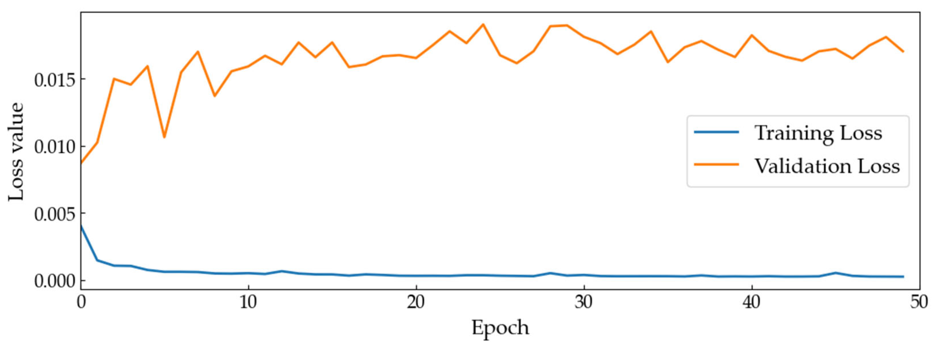
This step is then followed by the “Define Control Model Architecture” step. At this step, manual input is required from the user to set the deep learning model architecture. This entails specifying the number of layers, the type of network, optimization method, and number of epochs. Once the model structure has been defined, the training phase begins by utilizing the data that was prepared in the preceding step. This training will generate the deep learning-based control model.

The loss function is evaluated and, if it provides the expected result, the training process is terminated and the model will be evaluated in the “Model Validation” step. The model validation step employs data that has never been seen before. It is expected that the performance of the model during the validation process will be the same as that of the training model. However, it is very common that the model’s performance during the validation step is less than that of the training model, as it is hard to evaluate the model on unseen data. In this case, an engineering judgment is often required to terminate the iteration. These three steps, Define the Model Architecture, Train the Model, and Validate the Model, are an iterative process. The process will be terminated after the loss value produced by the model is as expected, or it can also be concluded via the engineering judgement. Sometimes, the process must be re-started from the data-gathering step because the trained model has not achieved the expected performance despite multiple iterations of modifying the model’s architecture. If this case arises, new data from a new experiment is needed and the process is repeated from the beginning.

Once the model achieves the expected level of performance, the developed model will be employed in the prediction step. This step involves predicting the output based on new data. Model prediction is the final stage of the deep learning-based control model development. The model obtained during this process is ready to deploy to the real system. For the case at hand, the final model is deployed in the X-Plane flight simulator and it is expected to perform its role as the controller for the UAV. Each of these steps will be further elaborated in detail in Section 3.

3. Control Model Development

3.1. Data Gathering

The data gathering for the deep learning-based flight control development is carried out using the X-Plane flight dynamics model, which allows for the systematic recording of various flight parameters. Figure 5 presents the simulated tilt-rotor unmanned aerial vehicle (UAV) within the X-Plane flight simulator environment. Figure 5a presents the UAV positioned on the designated runway, ready for takeoff. Figure 5b illustrates the UAV in a steady-state cruise phase, achieved via manual piloting. For the reader’s information, the modeling of the tilt-rotor UAV is not conducted in this X-Plane simulation environment. Rather, it was modeled in the Plane Maker, which is a sub-program of the X-Plane flight simulator.

Although the X-Plane flight simulator program may generate over two thousand parameters, only a subset of them will be employed in the deep learning-based flight control development. The X-Plane flight simulator program stores all these parameters’ addresses in a txt file named “dataref.txt”. This file is in the Resources/plugins directory within the X-Plane installation folder. In this paper, an open-source NASA plugin called X-Plane Connect, or XPC, is utilized to help with data collection [29]. Additionally, the plugin is also employed for sending control signals from the controller block to the X-Plane program. The XPC plugin allows users to develop the data recording interface in various programming languages. In this research, Python programming language is chosen for the respected purpose.

As already presented at the beginning of this paper, there will be three autopilot systems developed in this research, i.e., roll hold, attitude hold, and speed hold systems. Both attitude and speed hold systems will serve as holding systems for the attitude angle and speed at a constant value, while roll hold serves as a holding system for roll angle. The latter is an essential holding system, particularly for the present case, to support the pitch hold system. At the final stage, all these holding systems will be employed to support the altitude hold in which the purpose is to hold the altitude at a given altitude.

During the data-gathering stage, it is found that the aircraft model at hand is hard to control manually, particularly during the transition phase. To address this issue, a Proportional–Integral–Derivative (PID) controller is developed and employed to control the UAV during the hovering, transition, and cruise phases. Once the aircraft is in cruise mode, the data collection process starts. This process is repeated until all datasets are collected. Furthermore, the PID controller is also expected to minimize the intervention from human error during the data collection process. Three PID controllers are developed for this purpose, i.e., speed hold, altitude and pitch hold, and roll hold systems. In the speed hold system, indicated airspeed (IAS) is used as a feedback signal and compared with the reference airspeed. The difference between the reference and feedback signals is minimized by employing gains in proportional, integrator, and derivative blocks, and the resulted signal is used to control the throttle position. This throttle position is connected directly to the changes in the UAV airspeed. Figure 6 depicts the schematic diagram of the speed hold system.

The combined altitude and pitch hold system operates on the same basis, requiring appropriate parameter selection for the feedback signals. Typically, this system is referred to as an altitude hold system in an aircraft control development. To ensure its robustness, a pitch rate hold system is commonly utilized in the inner most loop, while the rest of the configuration is the same as the combined altitude and pitch hold system. These three loop combinations ensure the robustness of the altitude hold system. For the current combined holding system, pitch angle and altitude are used as feedback signals. Each of these hold systems has its own gains which are obtained based on a trial-and-error approach. The signal produced from this combined holding system is employed to control the ruddervator of the UAV. This holding system will maintain the altitude of the aircraft based on the reference altitude provided by the user.

The last PID controller developed for the data-gathering purpose is a roll hold system. This holding system is necessary for the data-gathering process, particularly during the cruise phase in which the deep learning-based controller will be developed. The feedback signal used for this roll hold system is the roll angle. The resulting signal of the controller will be used to control the rudder control surface. This roll hold system ensures that the UAV flies with zero roll angle during the cruise phase. Since the same principle is applied for the altitude and roll hold systems, the schematic diagrams for these holding systems are not presented here. All the controllers are implemented in Python programming language. The XPC plugin provides data needed by the controllers. Both the controller and the XPC plugin run within the X-Plane system, meaning that they will run as long as the X-Plane program is also running. The data-gathering process is started once the drone is in cruise phase. Many parameters are recorded at the same sampling rate of 50 Hz during the data collection stage. The recording process is terminated until all datasets are collected. The total datasets gathered is twenty-seven, of which twenty of them will be used for training purposes while the remaining seven datasets are for prediction. Figure 7 depicts some examples of time series parameters collected during this data-gathering step. For the data presented in Figure 7, no data preprocessing is employed yet.

3.2. Data Preprocessing

After the data is collected, the next step is to carry out the “Data Preprocessing” step. This step is necessary to ensure that the developed deep learning model works optimally. Since the collected data is a long time series data, the windowing process needs to be conducted. Windowing is a technique used to divide a time series dataset into smaller arrays with overlapping segments. By windowing the data, it ensures the deep learning model to learn temporal patterns and reduce computational complexity [30]. For instance, the time series of pitch angle data contains (0.0, 2.5, 2.7, 2.1, 2.4) and, after windowing with three windows, the data changes to ((0.0, 2.5, 2.7), (2.5, 2.7, 2.1), (2.7, 2.1, 2.4)). During the windowing process, the window size and overlap need to be carefully chosen in order to enhance the performance of the deep learning model.

3.3. Feature Selection and Feature Engineering

To reduce model complexity, prevent model overfitting, and improve model stability, the feature selection is a necessary step to be carried out [31]. Practically, feature selection is to reduce the number of parameters used during the model development. The physical interpretation of the parameters in relation to the motion of the drone serves as the foundation for parameter selection/feature selection. Furthermore, the selection of parameters is also conducted based on the type of flight control developed in this study. For example, the pitch angle parameter is selected since it has a direct correlation with the actual movement of the UAV.

As this study will develop an autopilot for the pitch hold system, this pitch angle parameter is also expected to be a feedback signal in the autopilot system. Hence, this parameter will be incorporated in the feature selection procedure. Additionally, to quantify the strength of the correlation among the parameters, a technique called correlation analysis, which is commonly used in the Deep Learning field, is employed in this research. The so-called Spearmen correlation is utilized for this purpose. The Spearmen correlation is used as it can detect both linear and non-linear correlation among the parameters. With the help of this correlation analysis, the selection of parameters to be incorporated in the model development is expected to be more robust and prevent model overfitting. Figure 8 depicts the correlation among the parameters based on the Spearman correlation coefficient.

As highlighted in Figure 8, we can observe that there is a strong correlation between certain output and input parameters. For example, the control column (yoke_pitch_ratio) has a strong correlation with the angle of attack (alpha) and elevation parameters with correlation coefficients of 0.72 and −0.63, respectively. For the data at hand, the control column (yoke_pitch_ratio) is expected to highly correlate with the pitch angle (theta) parameter. However, it is found that the correlation coefficient is 0.25, which is regarded as low. Nevertheless, from the physical point of view, these two parameters are expected to highly correlate as the main purpose of the control column is to control the attitude angle of the aircraft. Based on this physical interpretation, the pitch angle is still incorporated into the model development even though it has a low correlation coefficient. Feature engineering is carried out on two output parameters of elevation and indicated airspeed. Instead of using these two parameters directly in the model, their respected error is preferred as they provide more information to the model. The elevation is transformed into the altitude error which is obtained by subtracting the current altitude with the given reference value. The same procedure is also applied to obtain the airspeed error from the indicated airspeed parameter. The complete list of features used for the deep learning-based control model development is presented in

Table 3. Selected parameters employed for control model development.

Feature *	Unit	Description
engine_throttle	-	Throttle input for left and right engine, [−1 to 1]
yoke_pitch_ratio	-	Control column input, [−1 to 1]
yoke_roll_ratio	-	Yoke roller input, [−1 to 1]
alpha	deg	Angle of attack
beta	deg	Angle of sideslip
psi	deg	Yaw angle
phi	deg	Roll angle
theta	deg	Pitch angle
altitude_error	m	Current altitude subtracted by reference altitude
airspeed_error	m/s	Current airspeed subtracted by reference airspeed

* The variable name used in Python programming language.

.

3.4. Model Training and Validation

The control model development for the present case employs the TensorFlow framework [32]. This framework offers several advantages over other similar deep learning frameworks. Among these advantages are its maturity and stability, open-source framework, active and large community support, ease of use, and wide range of tools and libraries. The model architecture needs to be defined before the training process is carried out. The Long Short-Term Memory (LSTM) and dense layers are employed in the model architecture since both layers support well with the time series problem. While, in the activation function, the model architecture employs Relu and Linear functions. The output layer for the developed model consists of three neurons representing throttle, control column, and yoke roller parameters. Additionally, six dense hidden layers are utilized in the model architecture. The complete model architecture defined for the case at hand is presented in

Table 4. Deep learning-based control model architecture.

Layer	Number of Neuron	Activation Function
Normalization (input)	1	-
Bidirectional LSTM	64	-
Bidirectional LSTM	64	-
Bidirectional LSTM	64	-
Dense	128	Relu
Dense	128	Relu
Dense	64	Relu
Dense	64	Relu
Dense	32	Relu
Dense	32	Relu
Dense (output)	3	Linear

.

Furthermore, the loss function, optimizer, and epoch parameters are set to Huber Loss Function, Adam, and 50, respectively. The Huber loss function is preferred in the present case since it combines the mean squared error (MSE) and the mean absolute error (MAE). This combination makes this loss function less sensitive to outliers than MSE while it is still being differentiable. The model employs twenty datasets during the training and validation process. The Huber loss function is then evaluated to observe the performance of the model. Figure 9 depicts the result of the loss function for both the training and validation process.

As indicated in Figure 9, the training loss decreases rapidly at first but then slows down as the model approaches its best performance. Overall, it shows that the model fits well with the training data. However, the validation loss increases slightly at first and stays relatively constant throughout the remaining validation data. Compared to the training loss, the model does not perform well on this validation data. It is very common in data-driven modeling since the validation loss is measured on data that the model has never seen before. Despite the discrepancy between training and validation trends, the overall loss difference remains small. This suggests that the model performs adequately on unseen data, meeting acceptable criteria for model acceptance.

Further investigation will be carried out during the prediction step, in which the performance of the developed control model will be reevaluated and it will be decided whether to finally reject or accept the model.

3.5. Model Prediction

In this stage, the developed control model is employed on unseen data. The control signal generated by the model is compared with the actual data. The model’s performance is assessed by measuring the degree to which the control signal can accurately track the actual data. The challenge here is that the control model is employed on data that has never been seen by the model.

For the speed hold system, the throttle signal produced by the model is expected to follow the trend of the actual throttle signal. This comparison is depicted in Figure 10 (top figure). It can be observed that the predicted throttle signal closely tracks the actual throttle data, indicating that the deep learning model is able to accurately predict the throttle control signal. However, there are some discrepancies between the predicted and actual data, particularly at the beginning and end of the graph. As the differences are very small, the control model developed for the present case is regarded as good.

Furthermore, the control model for altitude hold is developed with the same procedure as presented previously. The aim is to develop a joystick control model which will be employed to control the elevator. To evaluate the performance of the model, the predicted pitch joystick data is compared to the actual data, see Figure 10 (middle figure). As indicated in Figure 10, the developed control model can closely track the actual data. There are a few outliers where the predicted yoke pitch ratio deviates from the actual yoke pitch ratio. However, these outliers are relatively small and do not significantly affect the overall accuracy of the model.

The last deep learning control model developed for the present case is the roll hold system. This holding system utilizes the roll angle as the feedback signal and the deep learning control model is trained to mimic the control data in order to hold the roll angle at the specified setpoint. This control model must be always activated along the pitch hold system. This is due to the fact that any movement in the longitudinal axis will be directly affecting the movement in the lateral axis. The performance of the control model developed for this holding system is assessed by comparing the control signal generated by the model and the actual data, see Figure 10 (bottom figure). As can be seen, the error between the predicted and actual control signals is generally small, particularly at the beginning of the graph. Despite discrepancies ranging from −0.008 to 0.006 corresponding to approximately 0.2 to 0.15 degrees of the actual aileron movement, these deviations are regarded as small within the context of the holding system’s performance. Consequently, the developed deep learning control model can be considered effective and suitable for the present application.

In the next section, the three controllers will be implemented in an X-Plane flight simulator environment.

4. Results

4.1. Implementation on X-Plane Flight Simulator

This section presents the implementation of the deep learning-based flight control model in an X-Plane flight simulator. The control model runs actively to control the drone within the X-Plane flight simulator. Two scenarios are specified to evaluate the performance of the control model. The first scenario is specified with the target altitude of 110 m. Once the drone achieves this setpoint, the target altitude is changed to 120 m.

The presented control model exhibits efficient altitude hold and setpoint tracking capabilities, as demonstrated in Figure 11a, where the x-axis represents the time history in second. The initial implementation commences with a UAV at 100 m. A target altitude of 110 m is then assigned, prompting the control model to initiate corrective actions. Through elevator deflection, the model controls the UAV, achieving the desired altitude. While some initial overshoot appears, the control system rapidly regulates the trajectory, ending at a stable altitude of 110 m until the second scenario triggers. To further evaluate the control model effectiveness, a second scenario is set in motion while the UAV holds at 110 m. The setpoint is abruptly adjusted to 120 m, challenging the model’s responsiveness. Once again, the control system demonstrates adeptness, utilizing appropriate control surface deflection to propel the UAV towards the new target altitude. Figure 11a visually confirms successful tracking of the second setpoint. For a comprehensive assessment of the control model’s performance, analyzing the corresponding altitude error is crucial. Figure 11b presents this error signal, revealing its minimal magnitude throughout the experiment. As evidenced by the middle and end parts of the figure, the error remains small, signifying accurate and precise altitude control by the model.

Furthermore, the effectiveness of the speed hold model was assessed by simultaneously evaluating the produced actual speed and the setpoint. Figure 11c illustrates the setpoint at 8 m/s, with the control model aiming to maintain the actual speed at this desired value. While slight deviations below the setpoint are observed, Figure 11d reveals a maximum error of less than 1 m/s. Consequently, considering the minimal error value, the developed control model demonstrates satisfactory performance for speed hold in this context.

Additionally, the performance of the roll hold system is evaluated by analyzing the deviation of the actual roll angle from the setpoint of 0 deg, Figure 11a. Following the altitude change to 110 m, a slight and transient deviation in the actual roll angle is observed, persisting until the end of the observation period. However, the magnitude of this deviation remains under 1 deg, indicating adequate performance of the developed roll hold model for the present case. It is worth noting that Figure 11 does not explicitly show the roll error since the setpoint is 0 deg and the figure already depicts the error itself.

4.2. Control Model Robustness Testing

To assess the robustness of the control model developed in this research, a new experiment, by introducing wind speed to the dynamics of the UAV, will be conducted in this section. Two wind conditions are tested, 0.8 m/s and 2 m/s. As already presented previously in the “Data Gathering” step, the data collected is free of wind disturbances; hence, the control model is developed based on wind-free data. Therefore, this experiment addresses the critical question of whether the control model, trained on wind-free data, possesses sufficient robustness to cope with realistic wind dynamics.

Prior to initiating the experiment, a step-function wind disturbance of 0.8 m/s, ten percent of the actual cruise speed, is introduced into the UAV model in the X-Plane flight simulator via the XPConnect interface. The experiment commenced with the control model already operational and actively piloting the UAV. As depicted in Figure 12a, scenario #1 involved introducing the aforementioned wind disturbance. Figure 12b,c demonstrates that the control model exhibited robust performance against external perturbation. While a slight overshoot is observed in the data, this phenomenon can be attributed to the concurrent change in altitude and the control model’s attempt to track the desired trajectory. This overshoot is further reflected in the generated signals for engine throttle, yoke pitch ratio, and yoke roll ratio, see Figure 12d,e. Interestingly, the wind disturbance’s sole impact on the input signals manifested as minor fluctuations around their respective steady-state values. In addition, the speed hold system keeps the actual speed at a new steady-state value that is slightly below the target speed, specifically less than 1 m/s. This small deviation is regarded as low and the model is still capable of providing an adequate control for the speed hold, as demonstrated in Figure 12c.

The second scenario introduces 2 m/s wind speed with a step-form to the UAV dynamics in the X-Plane flight simulator environment, as presented in Figure 13a. Similar to the first scenario, the control model demonstrated robustness to the external perturbation. As depicted in Figure 13b, the altitude hold model successfully tracked the new setpoint of 110 m. The speed hold system exhibited comparable performance, albeit with a minor deviation from the reference speed, remaining within 1 m/s, as shown in Figure 13c. The corresponding control inputs are depicted in Figure 13d–f. Compared to the first scenario, these inputs exhibit increased fluctuations, a deliberate response to counteract the wind disturbance. Nevertheless, the impact on the overall control performance is considered insignificant, as the model retains its ability to adequately control the UAV. The results obtained in this section will be further discussed in Section 5.

5. Discussion

As already presented in Section 4, two experiments are conducted to evaluate the performance of the developed control model. The initial scenario provided a baseline by assessing the model’s effectiveness under wind-free conditions. Subsequently, the second scenario introduced two distinct wind disturbances to the UAV dynamics, aiming to investigate the model’s robustness to realistic environmental perturbations. This sequential approach facilitated a comprehensive evaluation of both intrinsic performance and robustness to external interference.

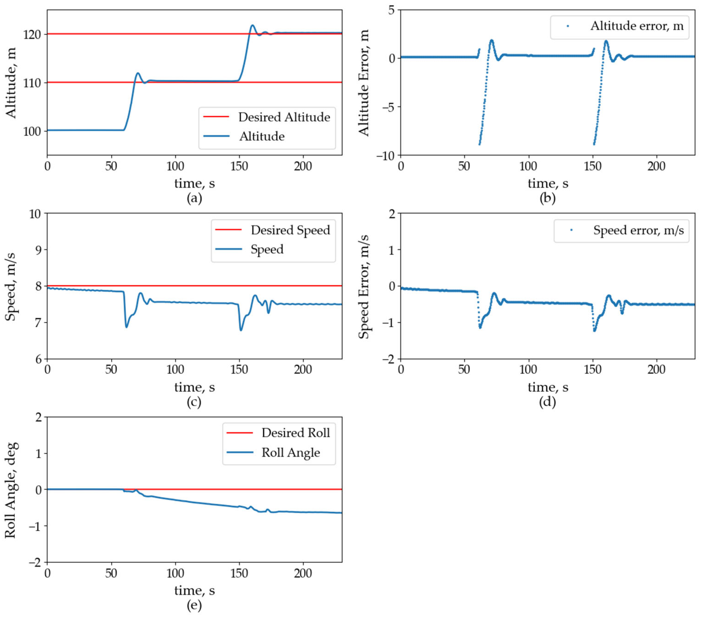
The first scenario assesses the performance of the control model by setting two altitude setpoints, where the first setpoint is 110 m, followed by 120 m. The UAV is initially placed at 100 m while the control model is actively controlling the UAV; as such, the first setpoint is altered. As presented in Figure 11, the control model is able to track the setpoint with a small overshoot at the beginning. For the remaining time of observation at this setpoint, the control model closely tracks the altitude. The speed hold system is also actively working to keep the speed at the setpoint of 8 m/s and its performance is also closely monitored by comparing the actual speed with the setpoint. As presented in Figure 11, the speed hold system provides an adequate performance as the deviation of the actual speed with the setpoint is small, specifically less than 1 m/s. Additionally, the roll hold model demonstrated satisfactory performance. While a transient deviation occurred upon setpoint change, the actual roll angle remained within one degree, indicating adequate roll control. Collectively, these results demonstrate the effectiveness of the deep learning-based control model under wind-free conditions.

Building upon the wind-free evaluation, the second scenario investigated the model’s robustness by introducing two distinct wind perturbations while the target altitude is set to 110 m. The first wind speed is set to ten percent of the cruise speed while the target altitude is introduced simultaneously with the setpoint change. Figure 13b illustrates the altitude hold system’s ability to effectively track the setpoint despite the external disturbance. Similarly, the speed hold system maintained satisfactory performance, as evidenced by the minimal deviation between actual and desired speeds, as presented in Figure 13c. Correspondingly, the generated inputs show small fluctuations due to the compensation of the external disturbances. Overall, as indicated in Figure 12, the control model exhibited robustness, suggesting its capability to handle realistic environmental disturbances without significant performance degradation.

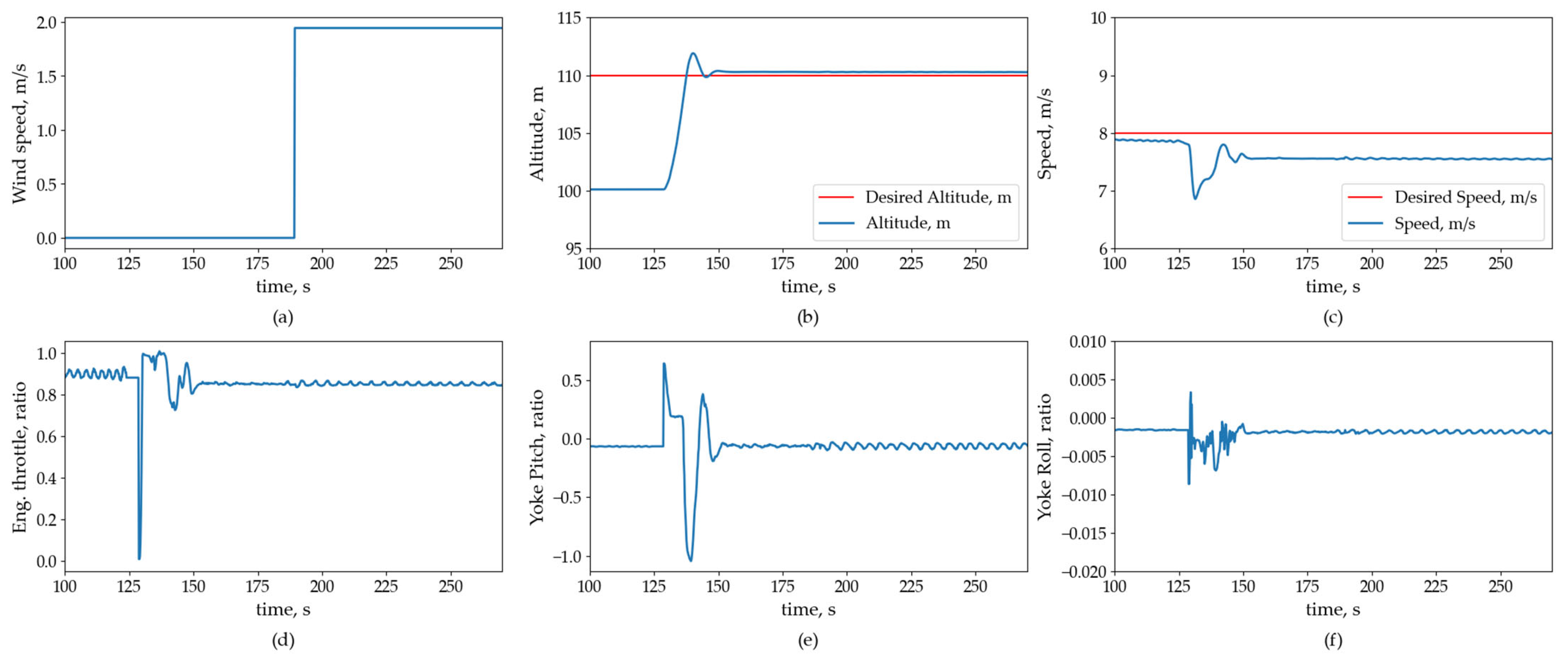
Further intensifying the evaluation, a 2 m/s step-function wind disturbance is introduced to the UAV dynamics, while simultaneously shifting the setpoint to 110 m, see Figure 13a. This triggered the control model to actively adjust its control strategies. As depicted in Figure 13b, the altitude hold system is capable of closely tracking the setpoint despite the external perturbation. Similarly, the speed hold system demonstrates satisfactory performance, evidenced by the minimal deviation between actual and desired speeds in Figure 13c. While a slight discrepancy of less than 1 m/s (to be within 6%) was observed between the target and actual speed, this deviation is regarded negligible within the context of the experiment. Analysis of the control and throttle inputs generated by the model, Figure 13d–f, reveals that the wind speed has minimal impact. Significant changes in these inputs only occur in response to the setpoint change, representing corrective actions to achieve the desired altitude. In conclusion, consistent with the previous scenario, the control model demonstrates its robustness to external disturbances, maintaining satisfactory performance under the 2 m/s wind perturbation.

Based on the investigation conducted in this paper, our research reveals some findings as presented shortly. In the context of the deep learning-based control model development, the quality of the data does significantly affect the performance of the control model. In this research, the quality of the training data is significantly improved by incorporating a PID controller during the data-gathering process. Additionally, the PID controller also helps in reducing the intervention of human error in controlling the UAV, particularly the tilt-rotor UAV at hand, which is naturally hard to control.

Secondly, the research highlights the crucial role of feature selection. While the deep learning approach possesses inherent feature selection capabilities, this can lead to significantly extended training times. Furthermore, the inclusion of many unrelated parameters during the training phase tends to produce models with overfitting performance. Some statistical measures, such as the correlation coefficient, can be employed to help in finding the most significant parameters to the model. Furthermore, modifications of features based on recorded features also contribute to a significant performance of the control model. The feature modification is facilitated via a so-called feature engineering in the context of Deep Learning field. For the present case, two additional features are incorporated in the training phase, i.e., altitude error and airspeed error, which capture the behavior of the system and contribute to the improvement of the control model significantly.

Finally, the investigation reveals the robustness of the developed control model. It is found that the deep learning-based control model, trained in wind-free conditions, provides a robust control model to withstand external disturbances, while intrinsically, it demonstrates its effectiveness in the wind-free condition.

Although the employed data were collected from an X-Plane flight simulator model, the developed deep learning-based control model demonstrates potential as an alternative control strategy for tilt-rotor UAVs, whose complex dynamic characteristics pose challenges compared to conventional fixed-wing UAVs. As future works, we plan to extend the flight phase control model development. The present work concentrates on control model development for the cruise flight phase. Future research works will focus on extending this to the more challenging transition phase. Furthermore, incorporating a data-driven flight dynamic model, estimated via System Identification of flight test data, is planned to improve the fidelity of the UAV flight dynamics model and allow for broader exploration of various flight phases.

6. Conclusions

The tilt-able configuration can provide a good combination of the flexibility of a rotorcraft and efficiency of a fixed-wing aircraft. However, this configuration inherently introduces complexities due to significant shifts in dynamic characteristics and behavior which require specific consideration and treatment, especially in relation to the control of its response and motion. The complexity of the dynamics behavior means that a set of complex equations is required for representing its dynamics, as well as to further be the basis for developing a closed-loop system. Data learning-based methods can be explored and employed for such situations, where data from “good practice” in controlling the system can be used for constructing the control parameter, instead of deriving it from the mathematical model. At the initial stage, even data from a numerical simulation process can be exploited for determining the structure of the controller and predicting the control parameters.

This paper successfully trained a deep learning-based flight control model utilizing X-Plane flight simulator data. Subsequent evaluation within the same environment demonstrated the model’s effectiveness in tracking desired setpoints with satisfactory performance. Under controlled wind-free conditions, the performance of the developed controller was evaluated via the application of two distinct setpoints. The results demonstrated the controller’s capability to effectively track both reference altitudes, showcasing its accurate and responsive feature. Furthermore, the robustness of the system was explored via its integrated hold systems, encompassing both speed and roll holds. These components displayed tracking fidelity, maintaining desired setpoints with minimal deviations, as evidenced by errors below 0.5 m/s for speed and 0.6 degrees for roll, respectively. The effectiveness of the control model extended beyond static wind-free scenarios, exhibiting a noteworthy degree of robustness against external disturbances. This robustness was further validated via simulations, introducing controlled wind speeds into the model. It was found that these simulations revealed insignificant impacts on the control model’s performance, with induced speed errors remaining within a modest 6% margin. These findings collectively prove the effectiveness and robustness of the developed deep learning-based control model, highlighting its potential for successful implementation in practical applications.

References

1. Capello, E.; Guglieri, G.; Quagliotti, F. A Design Configuration and Optimization for a Multi Rotor UAV. In Proceedings of the NATO RTO Symposium of Intelligent Uninhabited Vehicle Guidance Systems, Munich, Germany, 30 June–2 July 2009. [Google Scholar]
2. Department of the Air Force Washington DC. The U.S. Air Force Remotely Piloted Aircraft and Unmanned Aerial Vehicle Strategic Vision; Defense Technical Information Center: Fort Belvoir, VA, USA, 2005. [CrossRef]
3. Pinder, S. Control Strategy for a Four-Rotor VTOL UAV. In Proceedings of the 46th AIAA Aerospace Sciences Meeting and Exhibit; American Institute of Aeronautics and Astronautics, Reno, NV, USA, 7–10 January 2008. [Google Scholar] [CrossRef]
4. Lange, S.; Sünderhauf, N.; Protzel, P. Autonomous Landing for a Multirotor UAV Using Vision. In Proceedings of the International Conference on Simulation, Modeling, and Programming for Autonomous Robots (SIMPAR 2008), Venice, Italy, 3–4 November 2008. [Google Scholar]
5. Liu, Z.; He, Y.; Yang, L.; Han, J. Control techniques of tilt rotor unmanned aerial vehicle systems: A review. Chin. J. Aeronaut. 2016, 30, 135–148. [Google Scholar] [CrossRef]
6. Rysdyk, R.T.; Calise, A.J. Adaptive Model Inversion Flight Control for Tilt-Rotor Aircraft. J. Guid. Control Dyn. 1999, 22, 402–407. [Google Scholar] [CrossRef]
7. Lu, K.; Tian, H.; Zhen, P.; Lu, S.; Chen, R. Conversion Flight Control for Tiltrotor Aircraft via Active Disturbance Rejection Control. Aerospace 2022, 9, 155. [Google Scholar] [CrossRef]
8. Thirumaleshwar Hegde, N.; George, V.I.; Nayak, C.G.; Kumar, K. Transition Flight Modeling and Robust Control of a VTOL Unmanned Quad Tilt-Rotor Aerial Vehicle. Indones. J. Electr. Eng. Comput. Sci. 2020, 18, 1252. [Google Scholar] [CrossRef]
9. Kang, N.; Whidborne, J.; Lu, L.; Enconniere, J. Scheduled Flight Control System of Tilt-Rotor VTOL PAV. In Proceedings of the AIAA SCITECH 2023 Forum, National Harbor, MD, USA, 23–27 January 2023. [Google Scholar] [CrossRef]
10. Invernizzi, D.; Lovera, M. Geometric Tracking Control of A Quadcopter Tiltrotor UAV. IFAC-PapersOnLine 2017, 50, 11565–11570. [Google Scholar] [CrossRef]
11. Chen, Z.; Jia, H. Design of Flight Control System for a Novel Tilt-Rotor UAV. Complexity 2020, 2020, 4757381. [Google Scholar] [CrossRef]
12. Wen, J.; Song, Y.; Wang, H.; Han, D.; Yang, C. Hybrid Adaptive Control for Tiltrotor Aircraft Flight Control Law Reconfiguration. Aerospace 2023, 10, 1001. [Google Scholar] [CrossRef]
13. Chen, C.; Zhang, J.; Zhang, D.; Shen, L. Control and Flight Test of A Tilt-Rotor Unmanned Aerial Vehicle. Int. J. Adv. Robot. Syst. 2017, 14, 172988141667814. [Google Scholar] [CrossRef]
14. Abiodun, O.I.; Jantan, A.; Omolara, A.E.; Dada, K.V.; Mohamed, N.A.; Arshad, H. State-of-the-Art in Artificial Neural Network Applications: A Survey. Heliyon 2018, 4, e00938. [Google Scholar] [CrossRef]
15. Calise, A.J. Neural Networks in Nonlinear Aircraft Flight Control. IEEE Aerosp. Electron. Syst. Mag. 1996, 11, 5–10. [Google Scholar] [CrossRef]
16. Rysdyk, R.T.; Calise, D.A.J. Nonlinear Adaptive Control of Tiltrotor Aircraft Using Neural Networks. In Proceedings of the 1997 World Aviation Congress, Anaheim, CA, USA, 13–16 October 1997. [Google Scholar]
17. Taşören, A.E.; Gökçen, A.; Soydemir, M.U.; Şahin, S. Artificial Neural Network-Based Adaptive PID Controller Design for Vertical Takeoff and Landing Model. Eur. J. Sci. Technol. 2020, 2020, 87–93. [Google Scholar] [CrossRef]
18. Xi, L.; Shao, Y.; Zou, S.; Ma, Z. ADRC Based on Artificial Neural Network for a Six-Rotor UAV. In Proceedings of the 2021 40th Chinese Control Conference (CCC), Shanghai, China, 26–28 July 2021; IEEE: Shanghai, China, 2021; pp. 7809–7815. [Google Scholar] [CrossRef]
19. Abbaspour, A.; Yen, K.K.; Forouzannezhad, P.; Sargolzaei, A. A Neural Adaptive Approach for Active Fault-Tolerant Control Design in UAV. IEEE Trans. Syst. Man Cybern. Syst. 2020, 50, 3401–3411. [Google Scholar] [CrossRef]
20. Azar, A.T.; Koubaa, A.; Ali Mohamed, N.; Ibrahim, H.A.; Ibrahim, Z.F.; Kazim, M.; Ammar, A.; Benjdira, B.; Khamis, A.M.; Hameed, I.A.; et al. Drone Deep Reinforcement Learning: A Review. Electronics 2021, 10, 999. [Google Scholar] [CrossRef]
21. Dally, K. Deep Reinforcement Learning for Flight Control: Fault-Tolerant Control for the PH-LAB; TU Delft: Delft, The Netherlands, 2021; Available online: https://repository.tudelft.nl (accessed on 19 December 2023).
22. Koch, W. Flight Controller Synthesis via Deep Reinforcement Learning. arXiv 2019, arXiv:1909.06493. [Google Scholar]
23. d’Apolito, F.; Sulzbachner, C. Flight Control of a Multicopter using Reinforcement Learning. IFAC-PapersOnLine 2021, 54, 251–255. [Google Scholar] [CrossRef]
24. Koch, W.; Mancuso, R.; West, R.; Bestavros, A. Reinforcement Learning for UAV Attitude Control. ACM Trans. Cyber-Phys. Syst. 2019, 3, 1–21. [Google Scholar] [CrossRef]
25. Huo, Y.; Li, Y.; Feng, X. Tiltrotors Position Tracking Controller Design Using Deep Reinforcement Learning. IOP Conf. Ser. Mater. Sci. Eng. 2020, 751, 012047. [Google Scholar] [CrossRef]
26. Yang, R.; Du, C.; Zheng, Y.; Gao, H.; Wu, Y.; Fang, T. PPO-Based Attitude Controller Design for a Tilt Rotor Uav in Transition Process. Drones 2023, 7, 499. [Google Scholar] [CrossRef]
27. Flight Simulator|X-Plane 12: Flight Simulation Done Right. Available online: https://www.x-plane.com/ (accessed on 16 December 2023).
28. Bhanja, S.; Das, A. Impact of Data Normalization on Deep Neural Network for Time Series Forecasting. arXiv 2018, arXiv:1812.05519. [Google Scholar]
29. NASA/XPlaneConnect. NASA, 12 December 2023. Available online: https://github.com/nasa/XPlaneConnect (accessed on 16 December 2023).
30. Lim, B.; Zohren, S. Time Series Forecasting with Deep Learning: A Survey. Phil. Trans. R. Soc. A 2021, 379, 20200209. [Google Scholar] [CrossRef]
31. Li, J.; Cheng, K.; Wang, S.; Morstatter, F.; Trevino, R.P.; Tang, J.; Liu, H. Feature Selection: A Data Perspective. ACM Comput. Surv. 2018, 50, 1–45. [Google Scholar] [CrossRef]
32. TensorFlow. Available online: https://www.tensorflow.org/ (accessed on 18 December 2023).
Figure 1. The tilt-rotor UAV: (a) Tilt-rotor 3D model drawing; (b) the UAV conducted a flight test.
Aerospace 11 00096 g001
Figure 2. Tilt-rotor UAV flight phases. Started at hover flight (bottom figure) and followed by the transition phase (middle figure), and lastly, by the horizontal flight (top figure). The blue arrow represents the steps of the tilt-rotor flight, while the red arrow in the middle figure represents the tilting direction.
Aerospace 11 00096 g002
Figure 3. Tilt-rotor force–moment model.
Aerospace 11 00096 g003
Figure 4. Procedure of the deep learning-based control model development.
Aerospace 11 00096 g004
Figure 5. Tilt-rotor UAV modelled in X-Plane flight simulator: (a) On the runway, ready to takeoff, the main rotor in vertical position; (b) on cruise phase, the main rotor in horizontal position.
Aerospace 11 00096 g005
Figure 6. Schematic diagram of a PID controller for speed hold system.
Aerospace 11 00096 g006
Figure 7. Time—series of parameters collected during the data—gathering step.
Aerospace 11 00096 g007
Figure 8. Flight parameters’ correlation coefficient based on Spearman correlation approach. Red-framed part indicates the correlation coefficients of the selected parameters.
Aerospace 11 00096 g008
Figure 9. Huber loss results during training and validation process.
Aerospace 11 00096 g009
Figure 10. Comparison between actual vs. predicted data: (a) Predicted throttle and actual throttle; (b) predicted yoke pitch and actual yoke pitch; and (c) predicted yoke roll and actual yoke roll.
Aerospace 11 00096 g010
Figure 11. Control model implementation on X—Plane flight simulator: (a) Actual altitude and two setpoints; (b) corresponding altitude error; (c) actual speed compared with desired speed; (d) corresponding error of actual speed and desired speed; and (e) actual roll angle compared with desired roll angle. This figure also represents roll angle error as the setpoint is zero.
Aerospace 11 00096 g011
Figure 12. Control model implementation on X-Plane flight simulator, wind speed = 0.8 m/s: (a) Wind speed employed as a disturbance; (b) comparison of actual altitude with setpoint of 110 m; (c) comparison of actual speed and setpoint of 8 m/s; (d) generated engine throttle by the control model; (e) generated yoke pitch signal by the control model; and (f) generated yoke roll signal by the control model.
Aerospace 11 00096 g012
Figure 13. Control model implementation on X-Plane flight simulator, wind speed = 2 m/s: (a) Wind speed employed as a disturbance; (b) comparison of actual altitude with setpoint of 110 m; (c) comparison of actual speed and setpoint of 8 m/s; (d) generated engine throttle by the control model; (e) generated yoke pitch signal by the control model; and (f) generated yoke roll signal by the control model.
Aerospace 11 00096 g013