
Understanding How Image Quality Affects Transformer Neural Networks


Nokia Bell Labs, 1083 Budapest, Hungary
Signals 2024, 5(3), 562-579; https://doi.org/10.3390/signals5030031
Submission received: 8 July 2024
/
Revised: 15 August 2024
/
Accepted: 3 September 2024
/
Published: 5 September 2024
Abstract
:Deep learning models, particularly transformer architectures, have revolutionized various computer vision tasks, including image classification. However, their performance under different types and levels of noise remains a crucial area of investigation. In this study, we explore the noise sensitivity of prominent transformer models trained on the ImageNet dataset. We systematically evaluate 22 transformer variants, ranging from state-of-the-art large-scale models to compact versions tailored for mobile applications, under five common types of image distortions. Our findings reveal diverse sensitivities across different transformer architectures, with notable variations in performance observed under additive Gaussian noise, multiplicative Gaussian noise, Gaussian blur, salt-and-pepper noise, and JPEG compression. Interestingly, we observe a consistent robustness of transformer models to JPEG compression, with top-5 accuracies exhibiting higher resilience to noise compared to top-1 accuracies. Furthermore, our analysis highlights the vulnerability of mobile-oriented transformer variants to various noise types, underscoring the importance of noise robustness considerations in model design and deployment for real-world applications. These insights contribute to a deeper understanding of transformer model behavior under noisy conditions and have implications for improving the robustness and reliability of deep learning systems in practical scenarios.
1. Introduction
Visual quality evaluation in the context of computer vision refers to the process of assessing the perceived quality of digital images or digital videos generated by computer vision systems. This evaluation is critical for various applications, including image [1] and video processing [2], computer graphics [3], multimedia [4], and machine learning [5]. It involves quantifying the extent to which computer-generated visual content aligns with human perception, and it plays a pivotal role in ensuring the effectiveness and acceptability of computer vision applications [6].
One of the primary reasons for evaluating visual quality is to ensure that users are satisfied with the output of computer vision systems. Whether generating realistic images, enhancing photographs, or enabling virtual reality experiences, the quality of visual content significantly impacts user experience and engagement. High-quality visuals are more likely to be accepted and appreciated by users. Visual quality assessment aids decision-making processes in various industries. For instance, in medical imaging, accurate and high-quality visual representations are crucial for doctors to make informed diagnoses [7]. For example, in radiology, poor-quality images could lead to misdiagnosis or the failure to detect critical conditions such as tumors [8]. Visual quality evaluation ensures that images used in machine learning models for tasks like tumor detection have the necessary clarity and detail [9]. In autonomous driving, the quality of computer vision-based perception systems can determine the safety of the vehicle [10]. Namely, autonomous vehicles rely on cameras among others to interpret the environment around them. The quality of the images captured by these cameras directly affects the vehicle’s ability to detect and respond to obstacles [11]. Visual quality evaluation helps in filtering out poor-quality images that might introduce noise or errors ensuring that the algorithms work on clear and accurate images [12]. In multimedia applications, such as streaming video services or gaming, visual quality is a key factor [13]. Assessing and maintaining high-quality visuals ensures smooth content delivery, reduces buffering, and enhances the overall viewing experience for users [14]. In augmented reality (AR) and virtual reality (VR), visual quality also is paramount for immersion and user comfort. Poor-quality visuals can break immersion and even cause motion sickness [15]. For example, AR applications on mobile devices must constantly evaluate the visual quality of the environment they are augmenting to ensure smooth and accurate overlay of virtual objects [16]. This requires real-time visual quality evaluation to adjust rendering and processing based on environmental conditions. In machine learning, visual quality evaluation is essential for curating high-quality datasets. Annotated data used for training computer vision models must be of high visual quality to ensure accurate model performance. This is particularly important in applications like object recognition [17] and image segmentation [18]. In security applications, such as facial recognition systems, visual quality evaluation is essential for identifying individuals accurately [19]. In scenarios with low light or poor camera angles, the quality of the captured images may suffer, leading to false positives or negatives. Evaluating and ensuring high visual quality can mitigate these issues, leading to more reliable security systems. In manufacturing, computer vision systems are used to detect defects in products [20]. Visual quality evaluation ensures that images captured by inspection cameras are clear enough to detect even the smallest flaws. For example, in electronics manufacturing, even minor defects in circuit boards need to be detected, which requires high-quality image capture and analysis [21]. As can be seen from the above examples, visual quality evaluation is a cornerstone of effective computer vision applications. It ensures that the data used by models are of sufficient quality to produce reliable results and that the output meets the standards required for the specific use case.
In computer vision, neural network-based solutions and algorithms have achieved state-of-the-art results in a huge number of domains, i.e., image classification [22], image segmentation [23], action recognition [24], etc. In spite of their excellent performance in computer vision tasks, it was demonstrated that deep neural networks are sensitive to adversarial samples [25]. These adversarial samples are perturbations that are often imperceptible to humans, but they can significantly affect the model’s output. They can be generated using various techniques, including optimization algorithms that iteratively adjust the input to maximize the model’s prediction error [26,27]. In [28], Arjomandi et al. improved an adversarial attack against a stream of online images by implementing an optimization method to eliminate weight decay loss from the total loss term of models. Further, Dodge and Karam [29] pointed out that convolutional neural networks (CNNs) are very susceptible to certain distortion types and surprisingly resilient to JPEG or JPEG2000 compression noise.
1.1. Structure of the Paper
The rest of this paper is organized as follows. Section 1.2 reviews related and previous research work. In Section 1.3, the main contributions of this study are declared. Next, Section 2 introduces transformer networks in general and for computer vision tasks. The experimental setup used to evaluate the noise sensitivity of notable transformer models is presented in Section 3. Subsequently, Section 4 presents the obtained experimental results. Finally, a conclusion is drawn in Section 5.
1.2. Related Works
In the realm of computer vision, the ability of machines to interpret and understand visual information is paramount. However, this capability is significantly challenged by the presence of image noise, a ubiquitous phenomenon that arises from various sources. Image noise refers to random variations in pixel values that deviate from the true representation of the scene [30]. These variations can manifest as graininess, distortion, or irregular patterns in an image [31]. The sources of image noise are diverse, ranging from electronic sensor limitations in imaging devices to external factors like poor lighting conditions [32]. Regardless of the origin, the impact of image noise on computer vision algorithms is multifaceted and can impede the accuracy and reliability of visual information processing [1,33].
One of the primary challenges posed by image noise is its adverse effect on image analysis tasks. Computer vision algorithms often rely on precise pixel values to identify patterns, edges, and textures within an image. Image noise introduces spurious variations that can mislead these algorithms, leading to inaccurate feature extraction and compromising the overall quality of image analysis. As a consequence, tasks such as segmentation [34], image enhancement [35], and feature detection [36] become more challenging in the presence of noise. For instance, face recognition in low-quality images is a hot research topic in the literature [37]. Zou and Yuen [38] devised a face super-resolution method to reconstruct a higher resolution image for face recognition. In contrast, Li et al. [39] introduced the coupled mapping procedure, which first projects the images with different resolutions onto a lower dimensional space. Further, locality-preserving [40] was introduced in the optimization criterion to force identical labels as close as possible to each other in the new feature space.
1.3. Contributions
CNNs can be sensitive to certain types of noise, especially when the noise interferes significantly with the visual patterns and features that the network is trained to recognize. The impact of noise on CNNs depends on the nature and intensity of the noise, as well as the specific characteristics of the network and the task it is designed to perform. Adversarial noise is specifically crafted to deceive neural networks. Small, imperceptible perturbations added to input images can lead to misclassifications. In [29], Dodge and Karam empirically demonstrated that CNNs are susceptible to blur and Gaussian noise distortions, while being resilient to compression noise. The main contribution of this paper is a large-scale evaluation of transformer networks on natural images under different types and levels of image distortions. Specifically, the ImageNet database [41], which contains more than 1,000,000 images and 1000 semantic categories, were applied in our experiments. Namely, this dataset was augmented by applying several different distortion types. Subsequently, the performances of 22 state-of-the-art trained transformer networks on the ImageNet database [41] were measured and results reported on these distorted images.
2. Background
The transformer is a type of neural network architecture introduced by Vaswani et al. [42] in 2017. It was a breakthrough in the field of natural language processing (NLP) and machine translation. Unlike previous sequence-to-sequence models, the transformer model does not rely on recurrent neural networks (RNNs) or CNNs for sequential data processing. Instead, it is based entirely on attention mechanisms. The key components of the transformer architecture are the followings:
- Self-attention mechanism: it allows the model to weigh the importance of different words in a sequence when predicting a particular word. It can focus on different parts of the input sequence for each word in the output sequence. This is particularly useful for tasks involving long-range dependencies in the input data.
- Multi-head attention: To capture different aspects of the input sequence, the self-attention mechanism is extended to multiple heads, allowing the model to jointly attend to information from different representation subspaces.
- Positional encoding: Since the transformer does not inherently understand the order of the input sequence, positional encodings are added to the input embeddings to give the model information about the positions of the words in the sequence.
- Feed-forward neural networks: After the attention layers, the model uses feed-forward neural networks to process the information from the attention layer and produce the final output.
- Encoder and decoder stacks: The transformer model consists of an encoder stack and a decoder stack. The encoder processes the input sequence, while the decoder generates the output sequence. Both the encoder and decoder contain multiple layers of the components mentioned above.
The absence of sequential processing (like in RNNs) and the ability to attend to different parts of the input sequence simultaneously (through self-attention) make transformers highly parallelizable and efficient for training on large datasets. Transformers have become the foundation for many state-of-the-art models in NLP, including BERT [43] (bidirectional encoder representations from transformers), GPT [44] (generative pre-trained transformer), and T5 [45] (text-to-text transfer transformer), among others. They have also found applications in various other domains beyond NLP due to their flexibility and effectiveness in capturing complex patterns in data.
Transformers can be applied to various computer vision tasks, including image classification. While CNNs have traditionally been the go-to architecture for image-related tasks, recent research has shown that transformers can also achieve competitive results [46].
3. Experimental Setup
In this section, we describe the experimental setup used to evaluate the noise sensitivity of notable transformer models trained on the ImageNet dataset. First, we provide an overview of the transformer architectures considered in our study. Second, we outline the details of the used database sampled from the ImageNet dataset, including its size, content, and class distribution. Third, we discuss the types of image distortions that were applied to assess the robustness of the transformer models under various noise conditions. This comprehensive setup enables us to systematically evaluate the performance of transformer models across different noise types and levels, providing valuable insights into their noise sensitivity and robustness.
To evaluate the performance of the considered models under different noise conditions, we systematically apply common artificial distortions, i.e., additive Gaussian noise, multiplicative Gaussian noise, blur, salt-and-pepper noise, and JPEG compression, to the images and measure both top-1 and top-5 accuracies.
3.1. Transformers
The vision transformer [47] (ViT) was one of the pioneering works that applied the transformer architecture to images. Namely, it treats images as sequences of patches and processes them through transformer layers. The key features of ViT are (1) patch embeddings, where images are divided into fixed-size patches, linearly embedded, and then treated as tokens similar to words in NLP tasks; and the (2) transformer encoder, which utilizes transformer layers for capturing global dependencies among patches. ViT achieved competitive results on various image classification benchmarks and demonstrated the effectiveness of transformers in vision tasks.
Graham et al. [48] introduced LeViT, which uses a hybrid architecture that combines CNNs and transformers. Namely, it utilizes first a CNN block with -sized convolutional kernels. Next, the resulting output from this CNN block is passed to a hierarchical ViT. The authors aim was to optimize the trade-off between accuracy and efficiency in a high-speed regime by incorporating principles from both convolutional neural networks and attention-based architectures. LeViT significantly outperforms existing convnets and transformers in terms of the speed/accuracy tradeoff, achieving a 5 times faster inference speed than EfficientNet on CPU at 80% ImageNet top-1 accuracy. The architecture is a stack of transformer blocks with pooling steps to reduce the resolution of the activation maps, resembling classical convolutional architectures.
The Swin transformer [49] focuses on efficiently modeling long-range dependencies in images. The key features of Swin are the following: (1) Hierarchical transformer architecture: It introduces a hierarchical architecture where the image is first divided into non-overlapping patches, which are then further divided into smaller, overlapping patches. This hierarchical approach helps capture both local and global information effectively. (2) Shifted windows: Swin uses shifted windows for self-attention, allowing the model to efficiently handle long-range dependencies.
Mehta and Rastegari [50] introduced a lightweight transformer for mobile devices. Specifically, the proposed MobileViT (mobile vision transformer) architecture consists of the following elements. First, strided convolutions process the input image, which is followed by MobileNetV2-style [51] inverted residual blocks to downsample the resolution of the intermediate feature maps. Compact design is also achieved through techniques such as depthwise separable convolutions [52], group convolutions [53], and efficient attention mechanisms. These optimizations help reduce the number of parameters and computational operations required while preserving the model’s expressive power. MobileViT also introduces spatial tokenization, which partitions input images into smaller patches and processes them independently, further enhancing efficiency without compromising performance. Overall, MobileViT represents a trade-off between model size, computational efficiency, and performance, making it a compelling choice for applications where resource constraints are a primary concern, such as mobile image classification, object detection, and image segmentation tasks.
As pointed out in the literature [54,55], convolutions are very good at capturing low-level, local features in images. Motivated by this, convolutional vision transformer (CVT) [56] first applies a convolution-based projection for capturing spatial structures in an input image and for tokenization of image patches. To mimic the effects of CNNs’ spatial downsampling, CVT implements a hierarchical design by gradually decreasing the number of tokens and increasing the width of tokens at the same time.
The main factors that limit the inference speed of ViTs include the massive number of parameters, quadratic-increasing computation complexity with respect to token length, non-foldable normalization layers, and lack of compiler level optimizations. These factors contribute to the high latency of ViTs, making them impractical for real-world applications on resource-constrained hardware such as mobile devices and wearables. Additionally, patch embedding with large kernel and stride has been identified as a speed bottleneck on mobile devices, and the choice of token mixer and the implementation of reshape operations also impact the latency of ViTs. In [57], the authors introduce a new model called EfficientFormer, which aims to achieve high performance with low inference latency on mobile devices. The study focuses on revisiting the network architecture and operators used in ViT-based models and identifying inefficient designs. It proposes a dimension-consistent design paradigm for vision transformers and performs latency-driven slimming to obtain a series of final models dubbed EfficientFormer.
Shaker et al. [58] introduced a novel efficient additive attention mechanism designed to replace the quadratic matrix multiplication operations in self-attention with linear element-wise multiplications. This approach aims to address the computational complexity of self-attention, making it more practical for deployment on resource-constrained mobile devices. The efficient additive attention eliminates the need for expensive matrix multiplication operations and allows for linear complexity with respect to the input image resolution. By incorporating this mechanism, the authors introduce a series of models called SwiftFormer, which achieve state-of-the-art performance in terms of accuracy and mobile inference speed. The proposed efficient additive attention enables the usage of attention at all stages of the network, providing a more effective trade-off between accuracy and latency compared to existing methods.
Guo et al. [59] presented a novel linear attention mechanism named large kernel attention (LKA) designed for computer vision tasks. LKA leverages the strengths of both convolution and self-attention mechanisms, addressing their respective limitations. Namely, LKA decomposes a large kernel convolution into three components: depthwise convolution, depthwise dilation convolution, and pointwise convolution. This decomposition allows for capturing long-range dependencies with reduced computational cost and parameters. The visual attention network (VAN) was then introduced, leveraging LKA for feature extraction in a simple hierarchical structure.
We present a summary of notable transformer architectures used in our study, including their publication year, number of parameters, and memory footprint. This information, outlined in Table 1, provides insights into the characteristics and scale of the transformer models evaluated in our experiments. The publication year indicates the temporal context of each model’s development, while the number of parameters and memory footprint offer insights into their computational complexity and resource requirements.
3.2. Dataset
ImageNet [41] is a large-scale visual database designed for use in visual object recognition research. It was created by researchers at Stanford University and is widely used in the field of computer vision. The database contains millions of labeled images, covering a vast range of object categories. The test was carried out on a subset of ImageNet’s validation set, since the labels for the test set of ImageNet are not publicly available. The ImageNet Large-Scale Visual Recognition Challenge (ILSVRC) organizers have historically kept the labels of the test set private to prevent overfitting and to ensure that the competition remains fair and unbiased. To create a database for our experiments, we sampled the ImageNet validation database by randomly selecting 50 classes. From each of these classes, we then randomly chose 100 images, resulting in a database containing 5000 images.
3.3. Distortion Types
In the context of image processing, additive Gaussian distortion involves adding random values sampled from a Gaussian distribution to each pixel in an image. This process can simulate various real-world scenarios where noise is present, such as electronic sensor noise in cameras or transmission noise in communication channels. Mathematically, if represents the intensity of a pixel at coordinates in the original image, and represents the Gaussian noise at those coordinates, the distorted image can be expressed as [60]:
Here, is a random variable with values sampled from a Gaussian distribution. In our experiments, we adjusted the variance in from 0 to 0.3 in increments of 0.01.
Multiplicative Gaussian distortion in image processing involves introducing multiplicative noise to an image, where the noise values are sampled from a Gaussian distribution [61]. Unlike additive Gaussian distortion, which adds noise directly to the pixel values, multiplicative distortion multiplies the pixel values by a factor determined by Gaussian noise. Mathematically, if represents the intensity of a pixel at coordinates in the original image, and represents the Gaussian noise at those coordinates, the distorted image can be expressed as:
Here, is a random variable with values sampled from a Gaussian distribution. The term represents the multiplicative factor applied to the original pixel value. In our experiments, we adjusted the variance in from 0 to 0.3 in increments of 0.01.
A Gaussian blur is a common technique used to reduce image noise and detail. The mathematical definition involves applying a Gaussian function to the image, which effectively smooths it. The Gaussian function in two dimensions is given by:
where is the standard deviation, which determines the extent of the blur. Further, x and y are the distances from the origin in the horizontal and vertical axes, respectively. A larger results in a greater blur, as the Gaussian function spreads out more. Conversely, a smaller results in less blur, with the function more concentrated around the center. To apply this blur to an image, the Gaussian function is used as a convolution kernel. Each pixel in the image is replaced by a weighted average of its neighbors, with the weights given by the Gaussian function. This process smooths out rapid intensity variations, thereby blurring the image. In our experiments, we used sized kernels and we adjusted the standard variation from 0 to 5 in increments of 0.1.
Salt-and-pepper noise, often referred to as salt-and-pepper distortion, is a type of image noise that manifests as randomly occurring bright and dark pixels in an image [62]. The name “salt-and-pepper” is derived from the visual analogy of the white and black specks resembling grains of salt and pepper on food. In images affected by salt-and-pepper noise, some pixels are randomly assigned the maximum intensity value (white), while others are assigned the minimum intensity value (black). The rest of the pixels retain their original values. This type of noise can be caused by various factors, including errors in image acquisition, transmission, or storage. Mathematically, the salt-and-pepper distortion can be represented as follows:
Here, represents the original intensity of the pixel at coordinates , is the maximum intensity value (white), is the minimum intensity value (black), and p is the probability of a pixel being affected by salt-and-pepper noise. The process involves independently deciding for each pixel whether it should become white, black, or remain unchanged based on the specified probabilities. In our experiments, we adjusted the relative prevalence (density) of noisy pixels from 0 to 0.3 in increments of 0.01.
Joint Photographic Experts Group (JPEG) compression is a widely used method for reducing the file size of digital images [63]. It is a lossy compression technique, meaning that some image information is discarded to achieve higher compression ratios. The goal is to reduce file size while preserving visual quality to an acceptable extent. JPEG compression introduces distortion in images, and this distortion is commonly referred to as JPEG compression artifacts. The primary artifacts associated with JPEG compression include [64]: blocking artifacts, quantization artifacts, chrominance subsampling artifacts, ring effects, and high-frequency detail loss. The degree of distortion depends on the compression settings chosen (e.g., quality factor), and higher compression ratios generally result in more noticeable artifacts. While JPEG compression is highly effective for reducing file sizes, it may not be suitable for applications where preserving every detail is critical, such as medical imaging or certain professional photography scenarios. In such cases, lossless compression or other compression methods may be preferred. In our experiments, the quality level of JPEG compression was adjusted from 100 to 5 in decrements of 5. Further, the quality level from 5 to 1 was adjusted in decrements of 1.
4. Results
Top-1 accuracy and top-5 accuracy are performance metrics commonly used in image classification tasks, particularly in the context of evaluating models trained on datasets like ImageNet [41]. Top-1 accuracy is a straightforward metric that measures the percentage of test images for which the correct class label is predicted as the top (most probable) prediction by the model. If the predicted class label is the same as the ground truth (actual label), then the prediction is considered correct. The formula for calculating top-1 accuracy is:
Top-5 accuracy is a more lenient metric that considers a prediction to be correct if the correct class label is among the top 5 predictions made by the model in order of probability. This is particularly relevant for large-scale image classification tasks where an image may belong to a fine-grained category, and the model might correctly identify a closely related class. The formula for calculating top-5 accuracy is:
In both cases, “correct prediction” refers to the model’s prediction aligning with the ground truth label.
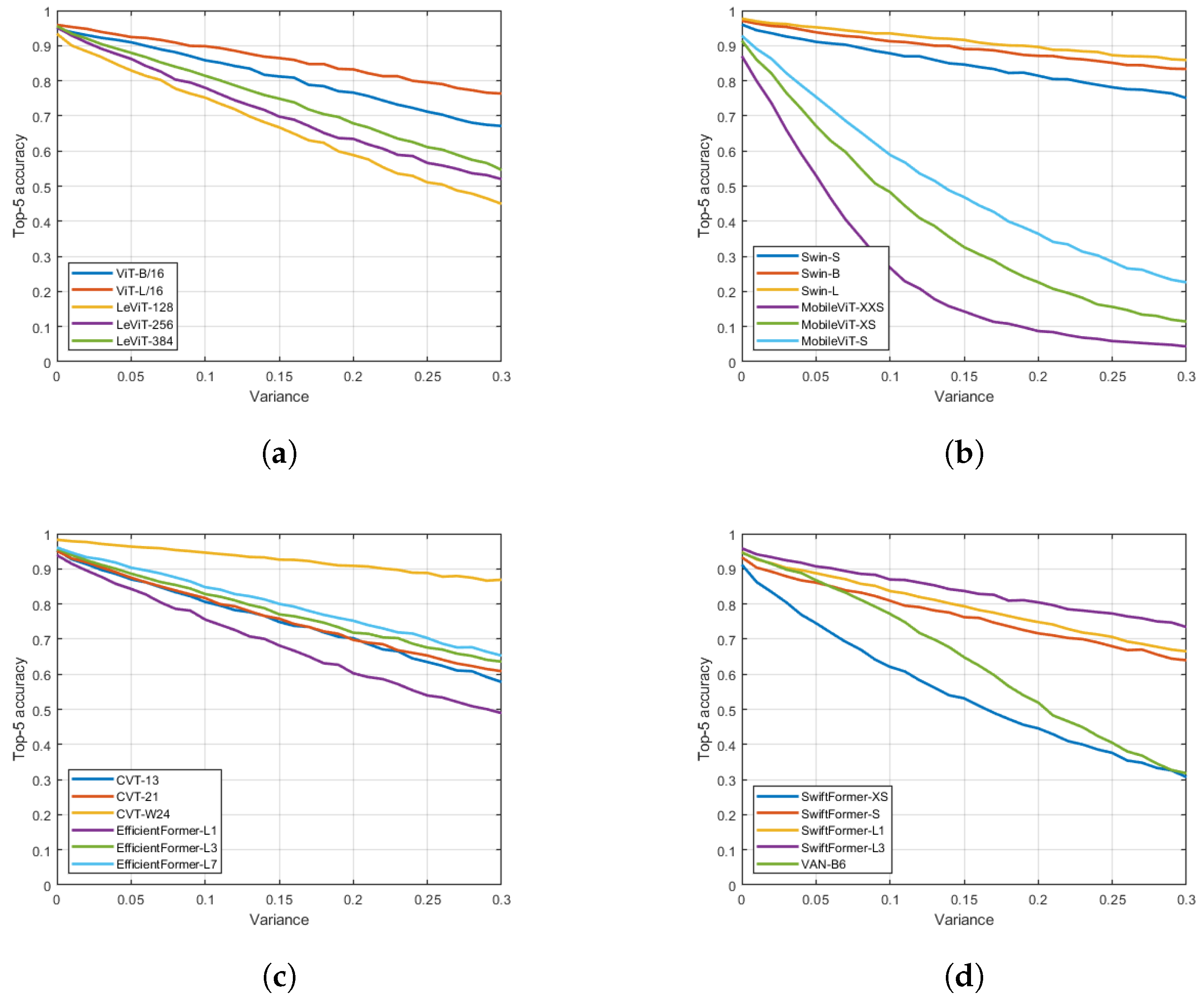
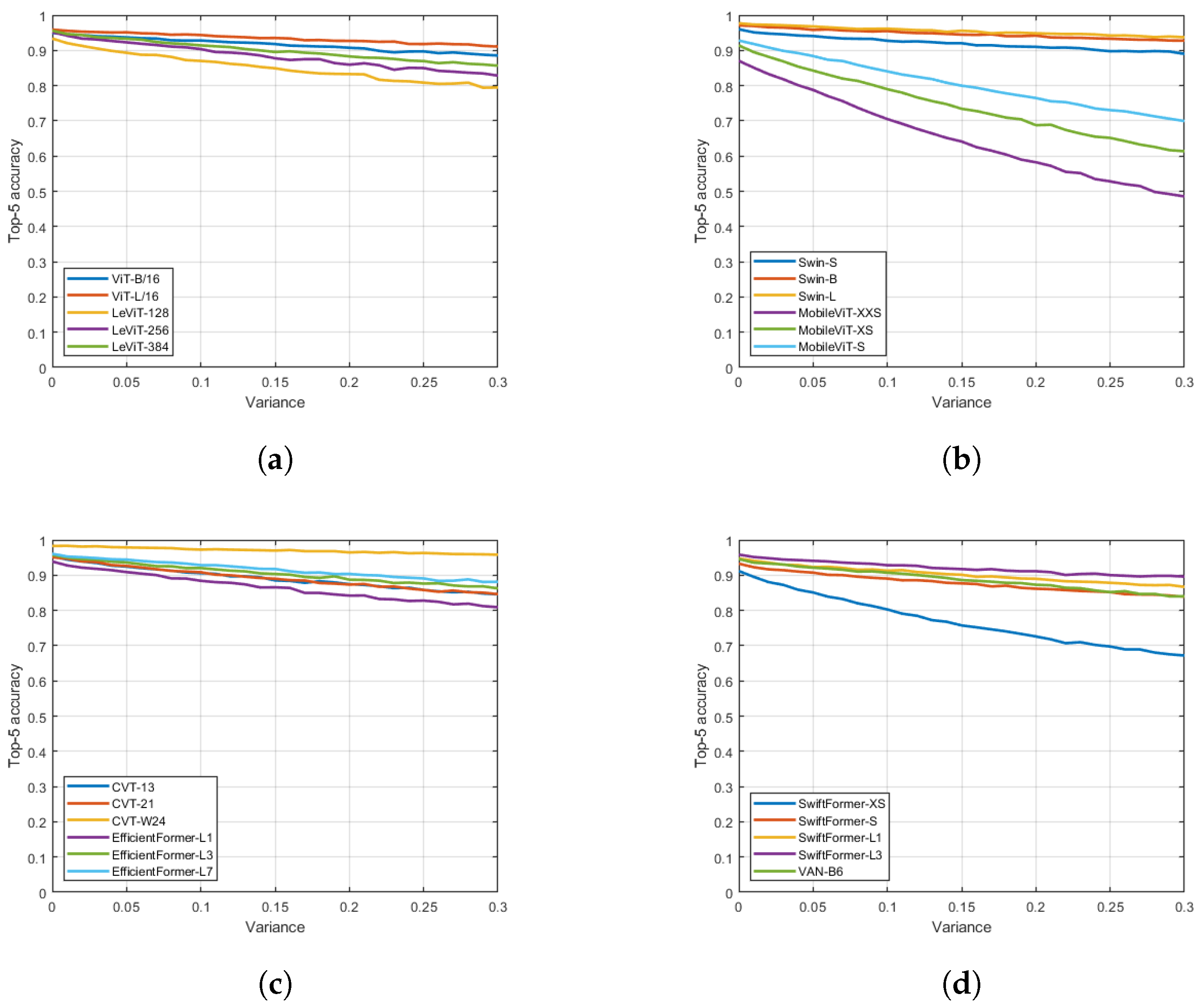
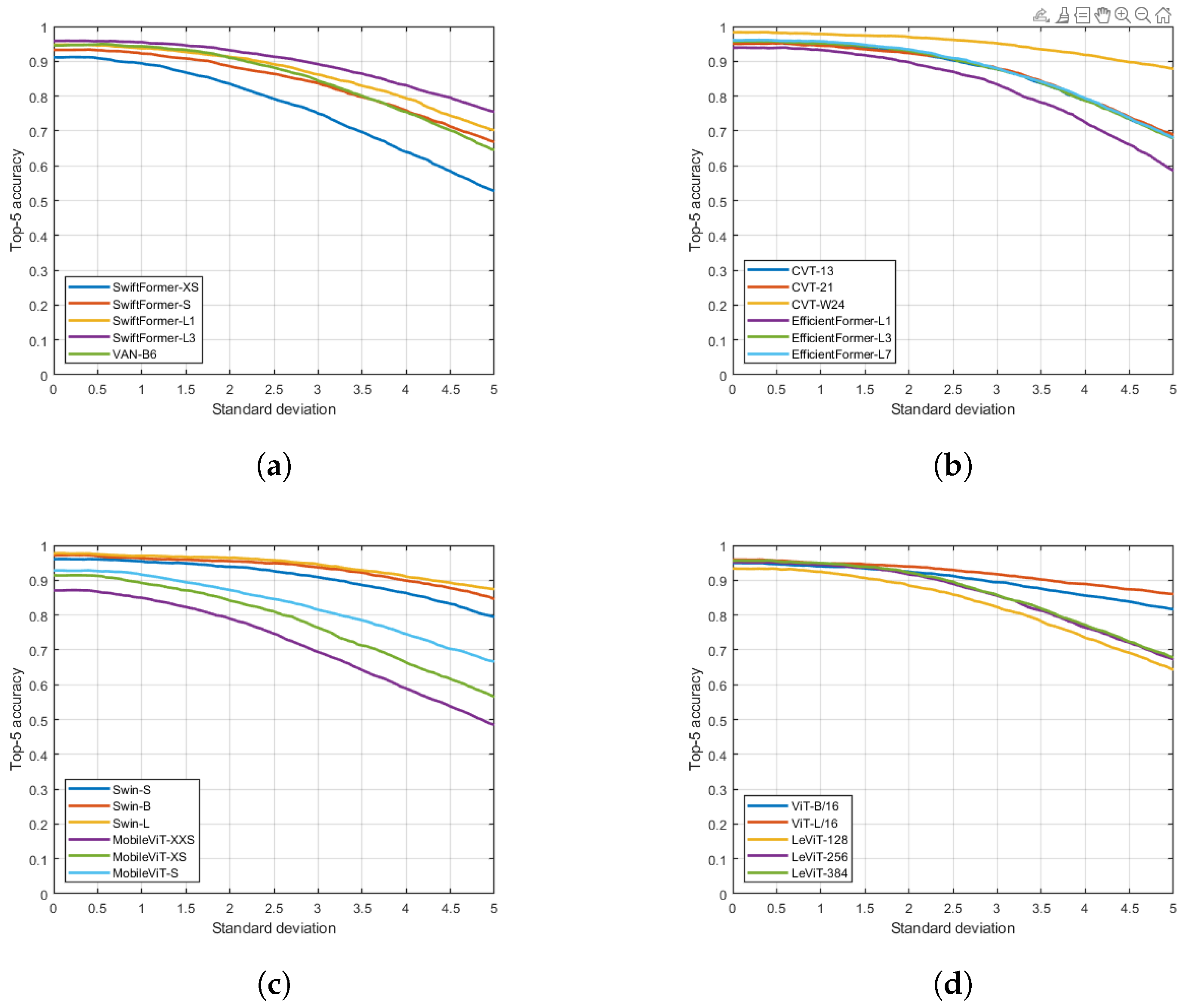
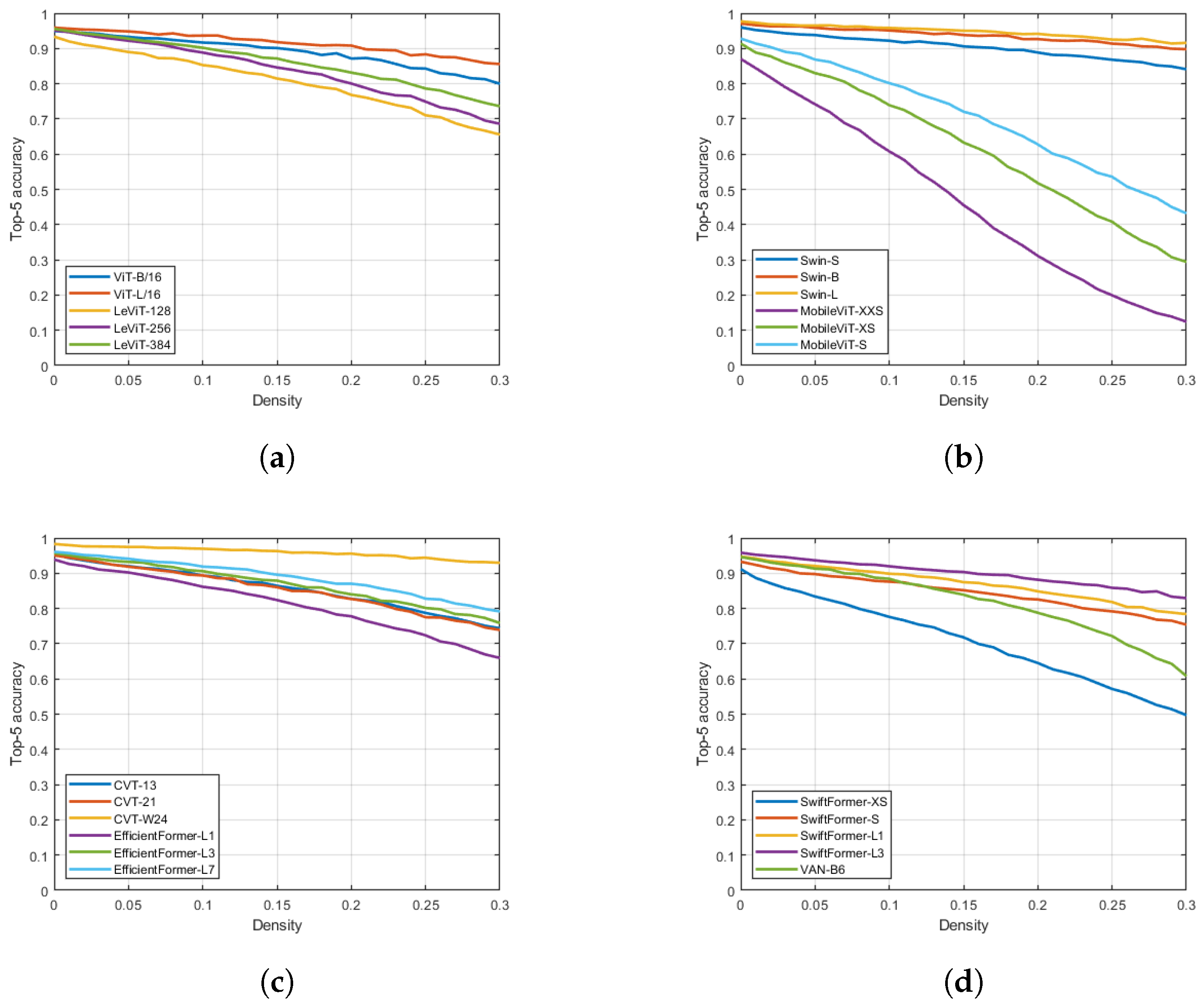
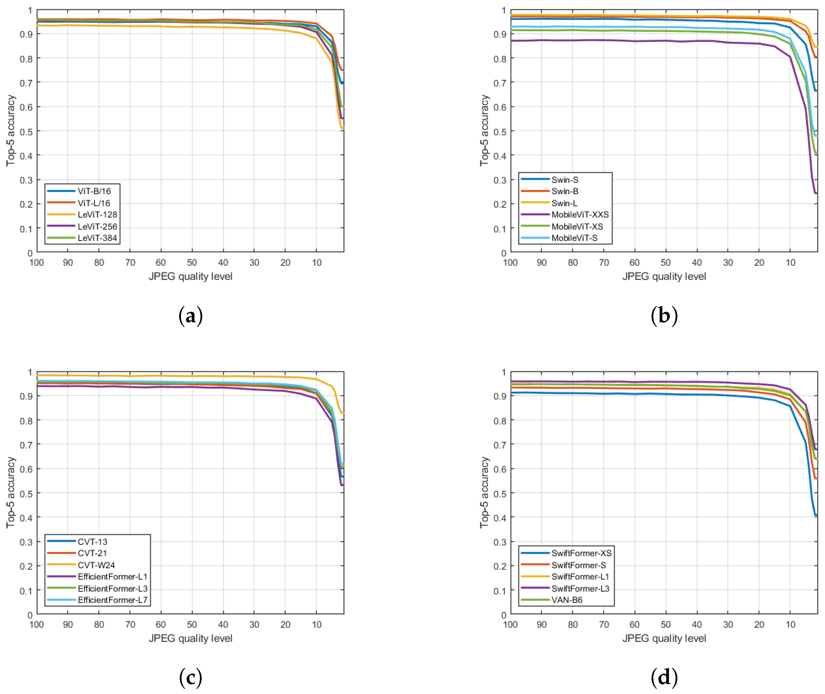
The numerical results of our experiments are summarized in Figure 1, Figure 2, Figure 3, Figure 4, Figure 5, Figure 6, Figure 7, Figure 8, Figure 9 and Figure 10. Specifically, top-1 accuracy values under five different distortion types with varying intensities are summarized in Figure 1, Figure 2, Figure 3, Figure 4 and Figure 5, while top-5 accuracy values can be seen in Figure 6, Figure 7, Figure 8, Figure 9 and Figure 10. From these figures, several conclusions can be drawn. First of all, various transformer networks exhibit distinct sensitives to noise. Even at moderate levels of noise, with the exception of JPEG compression, there is a noticeable decrease in top-1 accuracy performance across all transformer networks. This suggests that noise, regardless of intensity, generally impacts the performance of these networks, highlighting its significant influence on their robustness. The performance of transformers designed for mobile applications, such as MobileViT-XXS, MobileViT-XS, and MobileViT-S, exhibits exceptional sensitivity to various types of noise, with notable decreases observed in both top-1 and top-5 accuracy across all noise types, except for JPEG compression. This indicates a heightened vulnerability of these mobile-oriented transformers to noise interference, underscoring the need for robustness enhancements in such architectures. The outstanding sensitivity of mobile transformers to noise could be attributed to the following factors. Mobile transformers are typically designed to be lightweight and efficient to run on mobile devices with limited computational resources. This emphasis on efficiency may result in reduced model complexity compared to larger transformers, making them more susceptible to noise interference. The architectural choices made in designing mobile transformers, such as the size of the model, the number of layers, and the use of attention mechanisms, may not be optimized for noise robustness. Techniques like quantization and model compression, which are commonly employed to reduce the size of models for mobile deployment, can sometimes amplify the effects of noise, leading to decreased performance.
All transformers demonstrate high robustness to JPEG noise, maintaining stable top-1 and top-5 accuracies even up to 20% JPEG quality level. However, a sharp decrease in performance becomes evident at the 10% quality level. This indicates that JPEG noise has minimal impact on transformer performance until a certain threshold, beyond which there is a notable decline in accuracy. Namely, the JPEG compression algorithm primarily affects high-frequency components of an image, such as fine details and textures, while preserving low-frequency components, such as overall shapes and colors. This characteristic of JPEG compression often results in perceptually similar images despite significant compression, which may not significantly affect the performance of transformer models. Further, transformer models leverage self-attention mechanisms to capture long-range dependencies and relationships between different parts of an image. This allows them to focus on relevant features while disregarding irrelevant or noisy information. As a result, transformer models can effectively handle the distortions introduced by JPEG compression without significantly compromising performance.
From Figure 6, Figure 7, Figure 8, Figure 9 and Figure 10, it can be observed that top-5 accuracies are less sensitive to noise compared to top-1 accuracies. This could be explained by one important factor. As already mentioned, top-5 accuracy measures the percentage of test images for which the correct label is among the model’s top five predictions. This metric provides a more relaxed measure of performance and reflects the model’s ability to generalize and recognize the correct class among multiple plausible candidates. Therefore, even if the top-ranked prediction is affected by noise, the correct class may still be present within the top five predictions, leading to a higher top-5 accuracy. Most models are surprisingly robust against multiplicative Gaussian distortions both in terms top-1 and top-5 accuracies.
5. Conclusions
In this study, we evaluated the robustness of 22 state-of-the-art transformer models to five different types of image distortion: additive Gaussian noise, multiplicative Gaussian noise, Gaussian blur, salt-and-pepper noise, and JPEG compression noise. Our comprehensive analysis provides critical insights into how well these advanced models can maintain performance in the presence of various common distortions. Our results indicate a notable variance in robustness across the transformer models, with some models exhibiting significant resilience to certain noise types while others showed considerable degradation in performance. Additive and multiplicative Gaussian noise were particularly challenging for many models, leading to substantial performance drops. Conversely, the models handled JPEG compression artifacts very effectively. These findings highlight the importance of incorporating noise-specific augmentation techniques during the training phase to bolster model robustness. Future work should explore targeted training methodologies, incorporating a broader range of noise types and real-world distortions, to develop models that are not only accurate but also reliable in diverse and unpredictable environments. In summary, our study provides a valuable benchmark for the robustness of transformer models to image noise, offering guidance for future research and development in creating more resilient computer vision systems. By addressing the vulnerabilities identified in this analysis, we can enhance the practical applicability of these models in real-world scenarios where image quality can often be compromised.
In future work, we plan to extend our exploration of noise robustness to other computer vision tasks beyond image classification, including object detection, segmentation, and image generation. Additionally, it would be valuable to examine the practical implications of our findings, such as the development of noise-aware model selection or deployment strategies for real-world applications.
Funding
This research received no external funding.
Data Availability Statement
The data used in this study are available for download at https://huggingface.co/datasets/imagenet-1k (accessed on 1 August 2024). The experimental and numerical results supporting the findings of this study are available at https://github.com/elektrische-schafen/Understanding-How-Image-Quality-Affects-Transformer-Neural-Networks (accessed on 1 August 2024).
Acknowledgments
We would like to express our sincere gratitude to our colleague Krisztián Varga for his invaluable assistance and expertise in GPU computing. His guidance and support have been instrumental in optimizing our computational workflows and accelerating the progress of this research project. We would like to express our heartfelt gratitude to the entire team of Nokia Bell Labs, Budapest for fostering an environment of collaboration, support, and positivity throughout the duration of this project. We thank the anonymous reviewers and the academic editor for their careful reading of our manuscript and their many insightful comments and suggestions.
Conflicts of Interest
The authors declare no conflicts of interest.
Abbreviations
The following abbreviations are used in this manuscript:
| AR | augmented reality |
| BERT | bidirectional encoder representations from transformers |
| CNN | convolutional neural network |
| CVT | convolutional vision transformer |
| GPT | generative pre-trained transformer |
| ILSVRC | ImageNet large-scale visual recognition challenge |
| JPEG | joint photographic experts group |
| LKA | large kernel attention |
| MobileViT | mobile vision transformer |
| NLP | natural language processing |
| RNN | recurrent neural network |
| T5 | text-to-text transfer transformer |
| VAN | visual attention network |
| ViT | vision transformer |
| VR | virtual reality |
References
- Jenadeleh, M.; Pedersen, M.; Saupe, D. Blind quality assessment of iris images acquired in visible light for biometric recognition. Sensors 2020, 20, 1308. [Google Scholar] [CrossRef]
- Men, H.; Hosu, V.; Lin, H.; Bruhn, A.; Saupe, D. Subjective annotation for a frame interpolation benchmark using artefact amplification. Qual. User Exp. 2020, 5, 1–18. [Google Scholar] [CrossRef]
- Delepoulle, S.; Bigand, A.; Renaud, C. A no-reference computer-generated images quality metric and its application to denoising. In Proceedings of the 2012 6th IEEE International Conference Intelligent Systems, Sofia, Bulgaria, 6–8 September 2012; pp. 67–73. [Google Scholar]
- Saupe, D.; Hahn, F.; Hosu, V.; Zingman, I.; Rana, M.; Li, S. Crowd workers proven useful: A comparative study of subjective video quality assessment. In Proceedings of the QoMEX 2016: 8th International Conference on Quality of Multimedia Experience, Lisbon, Portugal, 6–8 June 2016. [Google Scholar]
- Men, H.; Lin, H.; Jenadeleh, M.; Saupe, D. Subjective image quality assessment with boosted triplet comparisons. IEEE Access 2021, 9, 138939–138975. [Google Scholar] [CrossRef]
- Götz-Hahn, F.; Hosu, V.; Lin, H.; Saupe, D. KonVid-150k: A Dataset for No-Reference Video Quality Assessment of Videos in-the-Wild. IEEE Access 2021, 9, 72139–72160. [Google Scholar] [CrossRef]
- Jenadeleh, M.; Pedersen, M.; Saupe, D. Realtime quality assessment of iris biometrics under visible light. In Proceedings of the IEEE Conference on Computer Vision and Pattern Recognition Workshops, Salt Lake City, UT, USA, 18–22 June 2018; pp. 443–452. [Google Scholar]
- Martin, C.; Sharp, P.; Sutton, D. Measurement of image quality in diagnostic radiology. Appl. Radiat. Isot. 1999, 50, 21–38. [Google Scholar] [CrossRef]
- Rosenkrantz, A.B.; Neil, J.; Kong, X.; Melamed, J.; Babb, J.S.; Taneja, S.S.; Taouli, B. Prostate cancer: Comparison of 3D T2-weighted with conventional 2D T2-weighted imaging for image quality and tumor detection. Am. J. Roentgenol. 2010, 194, 446–452. [Google Scholar] [CrossRef] [PubMed]
- Michaelis, C.; Mitzkus, B.; Geirhos, R.; Rusak, E.; Bringmann, O.; Ecker, A.S.; Bethge, M.; Brendel, W. Benchmarking robustness in object detection: Autonomous driving when winter is coming. arXiv 2019, arXiv:1907.07484. [Google Scholar]
- Wang, Z.; Zhao, D.; Cao, Y. Image Quality Enhancement with Applications to Unmanned Aerial Vehicle Obstacle Detection. Aerospace 2022, 9, 829. [Google Scholar] [CrossRef]
- Xin, L.; Yuting, K.; Tao, S. Investigation of the Relationship between Speed and Image Quality of Autonomous Vehicles. J. Min. Sci. 2021, 57, 264–273. [Google Scholar] [CrossRef]
- Zhu, K.; Asari, V.; Saupe, D. No-reference quality assessment of H. 264/AVC encoded video based on natural scene features. In Proceedings of the Mobile Multimedia/Image Processing, Security, and Applications, Baltimore, MS, USA, 29–30 April 2013; International Society for Optics and Photonics: San Francisco, CA, USA, 2013; Volume 8755, p. 875505. [Google Scholar]
- Kara, P.A.; Martini, M.G.; Kovács, P.T.; Imre, S.; Barsi, A.; Lackner, K.; Balogh, T. Perceived quality of angular resolution for light field displays and the validy of subjective assessment. In Proceedings of the 2016 International Conference on 3D Imaging (IC3D), Liege, Belgium, 13–14 December 2016; pp. 1–7. [Google Scholar]
- Chattha, U.A.; Janjua, U.I.; Anwar, F.; Madni, T.M.; Cheema, M.F.; Janjua, S.I. Motion sickness in virtual reality: An empirical evaluation. IEEE Access 2020, 8, 130486–130499. [Google Scholar] [CrossRef]
- Muthu Kumara Swamy, S.; Han, Q. Quality Evaluation of Image Segmentation in Mobile Augmented Reality. In Proceedings of the International Conference on Mobile and Ubiquitous Systems: Computing, Networking, and Services, Melbourne, VIC, Australia, 14–17 November 2023; Springer: Berlin/Heidelberg, Germany, 2023; pp. 415–427. [Google Scholar]
- Temel, D.; Lee, J.; AlRegib, G. Cure-or: Challenging unreal and real environments for object recognition. In Proceedings of the 2018 17th IEEE International Conference on Machine Learning and Applications (ICMLA), Orlando, FL, USA, 17–20 December 2018; pp. 137–144. [Google Scholar]
- Pednekar, G.V.; Udupa, J.K.; McLaughlin, D.J.; Wu, X.; Tong, Y.; Simone, C.B., II; Camaratta, J.; Torigian, D.A. Image quality and segmentation. In Proceedings of the Medical Imaging 2018: Image-Guided Procedures, Robotic Interventions, and Modeling, Houston, TX, USA, 12–15 February 2018; SPIE: Bellingham, WE, USA, 2018; Volume 10576, pp. 622–628. [Google Scholar]
- Galbally, J.; Marcel, S.; Fierrez, J. Image quality assessment for fake biometric detection: Application to iris, fingerprint, and face recognition. IEEE Trans. Image Process. 2013, 23, 710–724. [Google Scholar] [CrossRef]
- Zhou, L.; Zhang, L.; Konz, N. Computer vision techniques in manufacturing. IEEE Trans. Syst. Man, Cybern. Syst. 2022, 53, 105–117. [Google Scholar] [CrossRef]
- Pau, L.F. Computer Vision for Electronics Manufacturing; Springer Science & Business Media: Berlin/Heidelberg, Germany, 2012. [Google Scholar]
- Li, S.; Song, W.; Fang, L.; Chen, Y.; Ghamisi, P.; Benediktsson, J.A. Deep learning for hyperspectral image classification: An overview. IEEE Trans. Geosci. Remote. Sens. 2019, 57, 6690–6709. [Google Scholar] [CrossRef]
- Minaee, S.; Boykov, Y.; Porikli, F.; Plaza, A.; Kehtarnavaz, N.; Terzopoulos, D. Image segmentation using deep learning: A survey. IEEE Trans. Pattern Anal. Mach. Intell. 2021, 44, 3523–3542. [Google Scholar] [CrossRef]
- Koohzadi, M.; Charkari, N.M. Survey on deep learning methods in human action recognition. IET Comput. Vis. 2017, 11, 623–632. [Google Scholar] [CrossRef]
- Goodfellow, I.J.; Shlens, J.; Szegedy, C. Explaining and harnessing adversarial examples. arXiv 2014, arXiv:1412.6572. [Google Scholar]
- Szegedy, C.; Zaremba, W.; Sutskever, I.; Bruna, J.; Erhan, D.; Goodfellow, I.; Fergus, R. Intriguing properties of neural networks. arXiv 2013, arXiv:1312.6199. [Google Scholar]
- Zhang, M.; Chen, Y.; Qian, C. Fooling Examples: Another Intriguing Property of Neural Networks. Sensors 2023, 23, 6378. [Google Scholar] [CrossRef]
- Arjomandi, H.M.; Khalooei, M.; Amirmazlaghani, M. Low-epsilon adversarial attack against a neural network online image stream classifier. Appl. Soft Comput. 2023, 147, 110760. [Google Scholar] [CrossRef]
- Dodge, S.; Karam, L. Understanding how image quality affects deep neural networks. In Proceedings of the 2016 Eighth International Conference on Quality of Multimedia Experience (QoMEX), Lisbon, Portugal, 6–8 June 2016; pp. 1–6. [Google Scholar]
- Zhu, K.; Saupe, D. Performance evaluation of HD camcorders: Measuring texture distortions using Gabor filters and spatio-velocity CSF. In Proceedings of the Image Quality and System Performance X. International Society for Optics and Photonics, Burlingame, CA, USA, 4 February 2013; Volume 8653, p. 86530A. [Google Scholar]
- Zhu, K.; Li, S.; Saupe, D. An objective method of measuring texture preservation for camcorder performance evaluation. In Proceedings of the Image Quality and System Performance IX. International Society for Optics and Photonics, Burlingame, CA, USA, 24 January 2012; Volume 8293, p. 829304. [Google Scholar]
- Li, C.T. Source camera identification using enhanced sensor pattern noise. IEEE Trans. Inf. Forensics Secur. 2010, 5, 280–287. [Google Scholar]
- Su, S.; Lin, H.; Hosu, V.; Wiedemann, O.; Sun, J.; Zhu, Y.; Liu, H.; Zhang, Y.; Saupe, D. Going the Extra Mile in Face Image Quality Assessment: A Novel Database and Model. arXiv 2022, arXiv:2207.04904. [Google Scholar] [CrossRef]
- Ali, H.; Rada, L.; Badshah, N. Image segmentation for intensity inhomogeneity in presence of high noise. IEEE Trans. Image Process. 2018, 27, 3729–3738. [Google Scholar] [CrossRef]
- Rahman, Z.U.; Jobson, D.J.; Woodell, G.A.; Hines, G.D. Image enhancement, image quality, and noise. In Proceedings of the Photonic Devices and Algorithms for Computing VII, San Diego, CA, USA, 15 September 2005; SPIE: Bellingham, WE, USA, 2005; Volume 5907, pp. 164–178. [Google Scholar]
- Kim, Y.H.; Lee, J. Image feature and noise detection based on statistical hypothesis tests and their applications in noise reduction. IEEE Trans. Consum. Electron. 2005, 51, 1367–1378. [Google Scholar]
- Wang, Z.; Miao, Z.; Jonathan Wu, Q.; Wan, Y.; Tang, Z. Low-resolution face recognition: A review. Vis. Comput. 2014, 30, 359–386. [Google Scholar] [CrossRef]
- Zou, W.W.; Yuen, P.C. Very low resolution face recognition problem. IEEE Trans. Image Process. 2011, 21, 327–340. [Google Scholar] [CrossRef]
- Li, B.; Chang, H.; Shan, S.; Chen, X. Low-resolution face recognition via coupled locality preserving mappings. IEEE Signal Process. Lett. 2009, 17, 20–23. [Google Scholar]
- He, X.; Niyogi, P. Locality preserving projections. In Proceedings of the Advances in Neural Information Processing Systems 16 (Neural Information Processing Systems, NIPS 2003), Vancouver, BC, Canada, 8–13 December 2003. [Google Scholar]
- Krizhevsky, A.; Sutskever, I.; Hinton, G.E. Imagenet classification with deep convolutional neural networks. Adv. Neural Inf. Process. Syst. 2012, 25, 1097–1105. [Google Scholar] [CrossRef]
- Vaswani, A.; Shazeer, N.; Parmar, N.; Uszkoreit, J.; Jones, L.; Gomez, A.N.; Kaiser, Ł.; Polosukhin, I. Attention is all you need. In Proceedings of the 31st Conference on Neural Information Processing Systems (NIPS 2017), Long Beach, CA, USA, 4–9 December 2017. [Google Scholar]
- Alaparthi, S.; Mishra, M. Bidirectional Encoder Representations from Transformers (BERT): A sentiment analysis odyssey. arXiv 2020, arXiv:2007.01127. [Google Scholar]
- Zhu, Q.; Luo, J. Generative pre-trained transformer for design concept generation: An exploration. Proc. Des. Soc. 2022, 2, 1825–1834. [Google Scholar] [CrossRef]
- Mastropaolo, A.; Scalabrino, S.; Cooper, N.; Palacio, D.N.; Poshyvanyk, D.; Oliveto, R.; Bavota, G. Studying the usage of text-to-text transfer transformer to support code-related tasks. In Proceedings of the 2021 IEEE/ACM 43rd International Conference on Software Engineering (ICSE), Madrid, Spain, 22–30 May 2021; pp. 336–347. [Google Scholar]
- Khan, S.; Naseer, M.; Hayat, M.; Zamir, S.W.; Khan, F.S.; Shah, M. Transformers in vision: A survey. ACM Comput. Surv. CSUR 2022, 54, 1–41. [Google Scholar] [CrossRef]
- Dosovitskiy, A.; Beyer, L.; Kolesnikov, A.; Weissenborn, D.; Zhai, X.; Unterthiner, T.; Dehghani, M.; Minderer, M.; Heigold, G.; Gelly, S.; et al. An image is worth 16x16 words: Transformers for image recognition at scale. arXiv 2020, arXiv:2010.11929. [Google Scholar]
- Graham, B.; El-Nouby, A.; Touvron, H.; Stock, P.; Joulin, A.; Jégou, H.; Douze, M. Levit: A vision transformer in convnet’s clothing for faster inference. In Proceedings of the IEEE/CVF International Conference on Computer Vision, Montreal, QC, Canada, 11–17 October 2021; pp. 12259–12269. [Google Scholar]
- Liu, Z.; Lin, Y.; Cao, Y.; Hu, H.; Wei, Y.; Zhang, Z.; Lin, S.; Guo, B. Swin transformer: Hierarchical vision transformer using shifted windows. In Proceedings of the IEEE/CVF International Conference on Computer Vision, Montreal, QC, Canada, 11–17 October 2021; pp. 10012–10022. [Google Scholar]
- Mehta, S.; Rastegari, M. Mobilevit: Light-weight, general-purpose, and mobile-friendly vision transformer. arXiv 2021, arXiv:2110.02178. [Google Scholar]
- Sandler, M.; Howard, A.; Zhu, M.; Zhmoginov, A.; Chen, L.C. Mobilenetv2: Inverted residuals and linear bottlenecks. In Proceedings of the IEEE Conference on Computer Vision and Pattern Recognition, Salt Lake City, UT, USA, 18–22 June 2018; pp. 4510–4520. [Google Scholar]
- Guo, Y.; Li, Y.; Wang, L.; Rosing, T. Depthwise convolution is all you need for learning multiple visual domains. In Proceedings of the AAAI Conference on Artificial Intelligence, Honolulu, HI, USA, 27 January–1 February 2019; Volume 33, pp. 8368–8375. [Google Scholar]
- Zhang, T.; Qi, G.J.; Xiao, B.; Wang, J. Interleaved group convolutions. In Proceedings of the IEEE International Conference on Computer Vision, Venice, Italy, 22–29 October 2017; pp. 4373–4382. [Google Scholar]
- Yuan, K.; Guo, S.; Liu, Z.; Zhou, A.; Yu, F.; Wu, W. Incorporating convolution designs into visual transformers. In Proceedings of the IEEE/CVF International Conference on Computer Vision, Montreal, QC, Canada, 11–17 October 2021; pp. 579–588. [Google Scholar]
- Yoo, H.J. Deep convolution neural networks in computer vision: A review. IEIE Trans. Smart Process. Comput. 2015, 4, 35–43. [Google Scholar] [CrossRef]
- Wu, H.; Xiao, B.; Codella, N.; Liu, M.; Dai, X.; Yuan, L.; Zhang, L. Cvt: Introducing convolutions to vision transformers. In Proceedings of the IEEE/CVF International Conference on Computer Vision, Montreal, QC, Canada, 11–17 October 2021; pp. 22–31. [Google Scholar]
- Li, Y.; Yuan, G.; Wen, Y.; Hu, J.; Evangelidis, G.; Tulyakov, S.; Wang, Y.; Ren, J. Efficientformer: Vision transformers at mobilenet speed. Adv. Neural Inf. Process. Syst. 2022, 35, 12934–12949. [Google Scholar]
- Shaker, A.; Maaz, M.; Rasheed, H.; Khan, S.; Yang, M.H.; Khan, F.S. SwiftFormer: Efficient additive attention for transformer-based real-time mobile vision applications. In Proceedings of the IEEE/CVF International Conference on Computer Vision, Paris, France, 2–3 October 2023; pp. 17425–17436. [Google Scholar]
- Guo, M.H.; Lu, C.Z.; Liu, Z.N.; Cheng, M.M.; Hu, S.M. Visual attention network. Comput. Vis. Media 2023, 9, 733–752. [Google Scholar] [CrossRef]
- Liu, W.; Lin, W. Additive white Gaussian noise level estimation in SVD domain for images. IEEE Trans. Image Process. 2012, 22, 872–883. [Google Scholar] [CrossRef]
- Tourneret, J.Y. Detection and estimation of abrupt changes contaminated by multiplicative Gaussian noise. Signal Process. 1998, 68, 259–270. [Google Scholar] [CrossRef]
- Chan, R.H.; Ho, C.W.; Nikolova, M. Salt-and-pepper noise removal by median-type noise detectors and detail-preserving regularization. IEEE Trans. Image Process. 2005, 14, 1479–1485. [Google Scholar] [CrossRef]
- Rabbani, M.; Joshi, R. An overview of the JPEG 2000 still image compression standard. Signal Process. Image Commun. 2002, 17, 3–48. [Google Scholar] [CrossRef]
- Wang, Z.; Sheikh, H.R.; Bovik, A.C. No-reference perceptual quality assessment of JPEG compressed images. In Proceedings of the International Conference on Image Processing, Rochester, NY, USA, 22–25 September 2002; Volume 1, pp. I–I. [Google Scholar]
Figure 1.
Top-1 accuracy rates under different additive Gaussian distortions. (a) SwiftFormer-XS, SwiftFormer-S, SwiftFormer-L1, SwiftFormer-L3, VAN-B6. (b) CVT-13, CVT-21, CVT-W24, EfficientFormer-L1, EfficientFormer-L3, EfficientFormer-L7. (c) Swin-S, Swin-B, Swin-L, MobileViT-XXS, MobileViT-XS, MobileViT-S. (d) ViT-B/16, ViT-L/16, LeViT-128, LeViT-256, LeViT-384.

Figure 2.
Top-1 accuracy rates under different multiplicative Gaussian distortions. (a) SwiftFormer-XS, SwiftFormer-S, SwiftFormer-L1, SwiftFormer-L3, VAN-B6. (b) CVT-13, CVT-21, CVT-W24, EfficientFormer-L1, EfficientFormer-L3, EfficientFormer-L7. (c) Swin-S, Swin-B, Swin-L, MobileViT-XXS, MobileViT-XS, MobileViT-S. (d) ViT-B/16, ViT-L/16, LeViT-128, LeViT-256, LeViT-384.

Figure 3.
Top-1 accuracy rates under Gaussian blur. (a) SwiftFormer-XS, SwiftFormer-S, SwiftFormer-L1, SwiftFormer-L3, VAN-B6. (b) CVT-13, CVT-21, CVT-W24, EfficientFormer-L1, EfficientFormer-L3, EfficientFormer-L7. (c) Swin-S, Swin-B, Swin-L, MobileViT-XXS, MobileViT-XS, MobileViT-S. (d) ViT-B/16, ViT-L/16, LeViT-128, LeViT-256, LeViT-384.

Figure 4.
Top-1 accuracy rates under different salt-and-pepper distortions. (a) SwiftFormer-XS, SwiftFormer-S, SwiftFormer-L1, SwiftFormer-L3, VAN-B6. (b) CVT-13, CVT-21, CVT-W24, EfficientFormer-L1, EfficientFormer-L3, EfficientFormer-L7. (c) Swin-S, Swin-B, Swin-L, MobileViT-XXS, MobileViT-XS, MobileViT-S. (d) ViT-B/16, ViT-L/16, LeViT-128, LeViT-256, LeViT-384.

Figure 5.
Top-1 accuracy rates under different JPEG distortions. (a) SwiftFormer-XS, SwiftFormer-S, SwiftFormer-L1, SwiftFormer-L3, VAN-B6. (b) CVT-13, CVT-21, CVT-W24, EfficientFormer-L1, EfficientFormer-L3, EfficientFormer-L7. (c) Swin-S, Swin-B, Swin-L, MobileViT-XXS, MobileViT-XS, MobileViT-S. (d) ViT-B/16, ViT-L/16, LeViT-128, LeViT-256, LeViT-384.

Figure 6.
Top-5 accuracy rates under different additive Gaussian distortions. (a) SwiftFormer-XS, SwiftFormer-S, SwiftFormer-L1, SwiftFormer-L3, VAN-B6. (b) CVT-13, CVT-21, CVT-W24, EfficientFormer-L1, EfficientFormer-L3, EfficientFormer-L7. (c) Swin-S, Swin-B, Swin-L, MobileViT-XXS, MobileViT-XS, MobileViT-S. (d) ViT-B/16, ViT-L/16, LeViT-128, LeViT-256, LeViT-384.

Figure 7.
Top-5 accuracy rates under different multiplicative Gaussian distortions. (a) SwiftFormer-XS, SwiftFormer-S, SwiftFormer-L1, SwiftFormer-L3, VAN-B6. (b) CVT-13, CVT-21, CVT-W24, EfficientFormer-L1, EfficientFormer-L3, EfficientFormer-L7. (c) Swin-S, Swin-B, Swin-L, MobileViT-XXS, MobileViT-XS, MobileViT-S. (d) ViT-B/16, ViT-L/16, LeViT-128, LeViT-256, LeViT-384.

Figure 8.
Top-5 accuracy rates under Gaussian blur. (a) SwiftFormer-XS, SwiftFormer-S, SwiftFormer-L1, SwiftFormer-L3, VAN-B6. (b) CVT-13, CVT-21, CVT-W24, EfficientFormer-L1, EfficientFormer-L3, EfficientFormer-L7. (c) Swin-S, Swin-B, Swin-L, MobileViT-XXS, MobileViT-XS, MobileViT-S. (d) ViT-B/16, ViT-L/16, LeViT-128, LeViT-256, LeViT-384.

Figure 9.
Top-5 accuracy rates under different salt-and-pepper distortions. (a) SwiftFormer-XS, SwiftFormer-S, SwiftFormer-L1, SwiftFormer-L3, VAN-B6. (b) CVT-13, CVT-21, CVT-W24, EfficientFormer-L1, EfficientFormer-L3, EfficientFormer-L7. (c) Swin-S, Swin-B, Swin-L, MobileViT-XXS, MobileViT-XS, MobileViT-S. (d) ViT-B/16, ViT-L/16, LeViT-128, LeViT-256, LeViT-384.

Figure 10.
Top-5 accuracy rates under different JPEG distortions. (a) SwiftFormer-XS, SwiftFormer-S, SwiftFormer-L1, SwiftFormer-L3, VAN-B6. (b) CVT-13, CVT-21, CVT-W24, EfficientFormer-L1, EfficientFormer-L3, EfficientFormer-L7. (c) Swin-S, Swin-B, Swin-L, MobileViT-XXS, MobileViT-XS, MobileViT-S. (d) ViT-B/16, ViT-L/16, LeViT-128, LeViT-256, LeViT-384.


Table 1.
Considered transformer architectures.
| Architecture | Year | Number of Parameters | Memory Footprint in Bytes |
|---|---|---|---|
| ViT-B/16 [47] | 2020 | 86,567,656 | 346,270,624 |
| ViT-L/16 [47] | 2020 | 304,326,632 | 1,217,306,528 |
| LeViT-128 [48] | 2021 | 9,213,936 | 38,448,128 |
| LeViT-256 [48] | 2021 | 18,893,876 | 77,266,064 |
| LeViT-384 [48] | 2021 | 39,128,836 | 158,338,896 |
| Swin-S [49] | 2021 | 49,606,258 | 198,886,024 |
| Swin-B [49] | 2021 | 87,768,224 | 351,533,888 |
| Swin-L [49] | 2021 | 196,532,476 | 786,590,896 |
| MobileViT-XXS [50] | 2021 | 1,272,024 | 5,104,800 |
| MobileViT-XS [50] | 2021 | 2,317,848 | 9,305,440 |
| MobileViT-S [50] | 2021 | 5,578,632 | 22,363,808 |
| CVT-13 [56] | 2021 | 19,997,480 | 80,093,144 |
| CVT-21 [56] | 2021 | 31,622,696 | 126,658,712 |
| CVT-W24 [56] | 2021 | 277,196,392 | 1,109,323,744 |
| EfficientFormer-L1 [57] | 2022 | 12,289,928 | 49,306,864 |
| EfficientFormer-L3 [57] | 2022 | 31,406,000 | 125,934,952 |
| EfficientFormer-L7 [57] | 2022 | 82,229,328 | 329,429,000 |
| SwiftFormer-XS [58] | 2023 | 3,475,360 | 13,925,488 |
| SwiftFormer-S [58] | 2023 | 6,092,128 | 24,404,344 |
| SwiftFormer-L1 [58] | 2023 | 12,057,920 | 48,281,280 |
| SwiftFormer-L3 [58] | 2023 | 28,494,736 | 114,061,408 |
| VAN-B6 [59] | 2023 | 26,579,496 | 106,421,776 |
Disclaimer/Publisher’s Note: The statements, opinions and data contained in all publications are solely those of the individual author(s) and contributor(s) and not of MDPI and/or the editor(s). MDPI and/or the editor(s) disclaim responsibility for any injury to people or property resulting from any ideas, methods, instructions or products referred to in the content. |
© 2024 by the author. Licensee MDPI, Basel, Switzerland. This article is an open access article distributed under the terms and conditions of the Creative Commons Attribution (CC BY) license (https://creativecommons.org/licenses/by/4.0/).
Share and Cite
MDPI and ACS Style
Varga, D. Understanding How Image Quality Affects Transformer Neural Networks. Signals 2024, 5, 562-579. https://doi.org/10.3390/signals5030031
AMA Style
Varga D. Understanding How Image Quality Affects Transformer Neural Networks. Signals. 2024; 5(3):562-579. https://doi.org/10.3390/signals5030031
Chicago/Turabian StyleVarga, Domonkos. 2024. "Understanding How Image Quality Affects Transformer Neural Networks" Signals 5, no. 3: 562-579. https://doi.org/10.3390/signals5030031