Markov Chain Monte Carlo simulation sounds, admittedly, like a method better left to professional practitioners and the like; but please don’t let the esoteric name fool you. MCMC, as we like to call is, is a powerful yet deceptively simple technique that can be useful in problems ranging throughout science and engineering.

Since this promises to be a practical introduction, let’s skip the usual statistical jargon (and nonsense) about priors, posterior distributions and . Instead we will focus on a direct and intuitive demonstration.

Optimization

Let’s start by setting up a problem for us to solve. A frequently encountered class of problems found in science, engineering and even finance, is to minimize (or optimize) a value. For example, given that building a bridge is a rather pricey endeavour, civil engineers will attempt to minimize the length of the bridge so to keep the cost down. In a similar vein, a stock broker would love to estimate how high (or low) a stock will go so as to know when to buy and when to sell. These are the sorts of problems that optimization tries to solve.

The second example is actually quite pertinent to our discussion because unlike finding the shortest distance between two shores (where there can be a sure answer), most problems don’t have a guaranteed answer. In these cases we’re searching for a good enough solution, one where the trade off between time and accuracy is appropriate.

Markov Chain and Cost Functions

A Markov Chain is a special term for a certain class of processes that are essentially ‘memory-less’. What this means is that the evolution of the system does not depend on where the system has been. To illustrate this, consider a coin flip. At each flipping, their is a 50/50 chance for eith side to land upright. This is a Markov process. Now something which would not fulfill this criteria might be the spread of the flu. When trying to predict how many people will suffer the flu in the next week, you better take into account how many people had the flu right now. With the flu, the past trends are quite helpful in predicting the course of future events, but in the Markov process of a coin flip is doesn’t help at all.

In the case of a coin flip, we’ve already discussed the idea of a cost function without even knowing it. When we said the coin had a 50/50 chance of landing heads, we intuitively realized that a heads-up flip and a tails-up flip are equally difficult for the coin. If you were a fair coin, you wouldn’t care which way you land. So a Cost Function is simply a black box (for all we care) that tells us how costly a certain outcome, such as when deciding how best to avoid traffic on the way to work. For a coin this cost function is flat, or indifferent to either outcome.

This cost function tells the Markov Chain how to evolve in time by describing the weights associated with each option. Going back to the optimization that we talked about before, the cost function should always point us in the right direction in terms of providing a better and better solution as time goes on. But enough of all this talking, let’s get right into it.

Let’s first setup a domain, or area, to explore. We’ll use a well known test function that should provide the complexity we require.

test = function (x,y) {
    return(-20*exp(-0.2*sqrt((x^2+y^2)/2))-exp(0.5*(cos(2*pi*x)+cos(2*pi*y)))+22.71828 )
}

library(lattice)
points = matrix(nrow=61, ncol=61, seq(-3,3,0.1)) ## Test points for plotting
filled.contour(x=points[,1], y=points[,1], z =test(points,t(points)), nlevels=20)

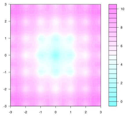
The test function is the mathematical surface that we’ll use to setup our domain. As seen in the contour plot, the function is topographically complex and offers many minimums (but only one global minimum at 0,0).

Here is an example of a cost function. This function compares the misfit between the new solution and the old solution to determine how much an improvement (or digression) the new solution offers.

accept = function(x1, y1, x2, y2) {
    score1 = test(x1,y1)
    score2 = test(x2,y2)
    if (exp(-15*(score2-score1)) > runif(1) ) {  ## is score > random number?
        return(TRUE)  ## Accept new solution
    }
    return(FALSE)  ## Reject new solution
}

If the new solution costs less than the old solution then it is guaranteed to be accepted and a poorer solution is unlikely to be accepted (but it can be, and that is important!).

For the MCMC method, we’ll start at a random point in the domain and then take steps based on whether or not the score is good enough (based on the accept function above). We’ll save all the steps we take in the MCMC with a dataframe (i.e. table) so we can plot the evolution over time.

x = runif(1,-1,1)
y = runif(1, -1,1)
position = data.frame(x,y)
position

Now we just have to setup the MCMC algorithm to use our starting point and the acceptance function. The jump length is simply how far from the current position the algorithm will search, and iter is the number of steps to take.

jmp = 0.2
iter = 50000
naccepted = 1

x = runif(1,0,2)
x = 2.3
y = runif(1, 0,2)
y = 1.98
position = data.frame(x,y)

for (i in 1:iter) {
    n = length(position[,1])
    new_x = rnorm(1, position[n,1], jmp)
    new_y = rnorm(1, position[n,2], jmp)
    
    if (accept( position[n,1], position[n,2],new_x, new_y )) {
        position[n+1,1] = new_x
        position[n+1,2] = new_y
        naccepted = naccepted + 1
    }   
}
print("Number accepted")
naccepted
print("Ratio of acceptance:")
naccepted/iter

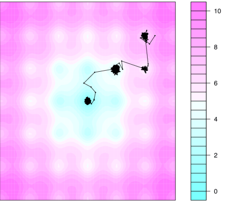
If we let it run, this is what we get:

The first point is at the top right and then as time went on the chain moved down into the local minimum right next to it. And then it climbed out of it eventually and fell into a better minimum and another before finally reaching the global minimum in the center.

Depending on how we choose the parameters, especially the cost function, the behavior and properties of the algorithm can change. Sometimes we’d want to explore the space more fully and therefore have a relatively relaxed cost function and a larger number of steps. Other times we just want a computationally cheap and quick solution for which we would use another combination of parameters.

MCMC methods are especially useful in higher dimensional cases (here ) such as for my inverse modeling research (see here) where or more.