Abstract
Consider the representative task of designing a distributed coin-tossing protocol for n processors such that the probability of heads is \(X_0\in [0,1]\). This protocol should be robust to an adversary who can reset one processor to change the distribution of the final outcome. For \(X_0=1/2\), in the information-theoretic setting, no adversary can deviate the probability of the outcome of the well-known Blum’s “majority protocol” by more than \(\frac{1}{\sqrt{2\pi n}}\), i.e., it is \(\frac{1}{\sqrt{2\pi n}}\) insecure.
In this paper, we study discrete-time martingales \((X_0,X_1,\dotsc ,X_n)\) such that \(X_i\in [0,1]\), for all \(i\in \{0,\dotsc ,n\}\), and \(X_n\in {\{0,1\}} \). These martingales are commonplace in modeling stochastic processes like coin-tossing protocols in the information-theoretic setting mentioned above. In particular, for any \(X_0\in [0,1]\), we construct martingales that yield \(\frac{1}{2}\sqrt{\frac{X_0(1-X_0)}{n}}\) insecure coin-tossing protocols. For \(X_0=1/2\), our protocol requires only 40% of the processors to achieve the same security as the majority protocol.
The technical heart of our paper is a new inductive technique that uses geometric transformations to precisely account for the large gaps in these martingales. For any \(X_0\in [0,1]\), we show that there exists a stopping time \(\tau \) such that

The inductive technique simultaneously constructs martingales that demonstrate the optimality of our bound, i.e., a martingale where the gap corresponding to any stopping time is small. In particular, we construct optimal martingales such that any stopping time \(\tau \) has

Our lower-bound holds for all \(X_0\in [0,1]\); while the previous bound of Cleve and Impagliazzo (1993) exists only for positive constant \(X_0\). Conceptually, our approach only employs elementary techniques to analyze these martingales and entirely circumvents the complex probabilistic tools inherent to the approaches of Cleve and Impagliazzo (1993) and Beimel, Haitner, Makriyannis, and Omri (2018).
By appropriately restricting the set of possible stopping-times, we present representative applications to constructing distributed coin-tossing/dice-rolling protocols, discrete control processes, fail-stop attacking coin-tossing/dice-rolling protocols, and black-box separations.
The research effort is supported in part by an NSF CRII Award CNS–1566499, an NSF SMALL Award CNS–1618822, the IARPA HECTOR project, MITRE Innovation Program Academic Cybersecurity Research Award, a Purdue Research Foundation (PRF) Award, and The Center for Science of Information, an NSF Science and Technology Center, Cooperative Agreement CCF–0939370.
You have full access to this open access chapter, Download conference paper PDF
1 Introduction
A Representative Motivating Application. Consider a distributed protocol for n processors to toss a coin, where processor i broadcasts her message in round i. At the end of the protocol, all processors reconstruct the common outcome from the public transcript. When all processors are honest, the probability of the final outcome being 1 is \(X_0\) and the probability of the final outcome being 0 is \(1-X_0\), i.e., the final outcome is a bias-\(X_0\) coin. Suppose there is an adversary who can (adaptively) choose to restart one of the processors after seeing her message (i.e., the strong adaptive corruptions model introduced by Goldwasser, Kalai, and Park [20]); otherwise her presence is innocuous. Our objective is to design bias-\(X_0\) coin-tossing protocols such that the adversary cannot change the distribution of the final outcome significantly.
The Majority Protocol. Against computationally unbounded adversaries, (essentially) the only known protocol is the well-known majority protocol [5, 10, 13] for \(X_0=1/2\). The majority protocol requests one uniformly random bit from each processor and the final outcome is the majority of these n bits. An adversary can alter the probability of the final outcome being 1 by \(\frac{1}{\sqrt{2\pi n}}\), i.e., the majority protocol is \(\frac{1}{\sqrt{2\pi n}}\) insecure.
Our New Protocol. We shall prove a general martingale result in this paper that yields the following result as a corollary. For any \(X_0\in [0,1]\), there exists an n-bit bias-\(X_0\) coin-tossing protocol in the information-theoretic setting that is \(\frac{1}{2}\sqrt{\frac{X_0(1-X_0)}{n}}\) insecure. In particular, for \(X_0=1/2\), our protocol uses only 625 processors to reduce the insecurity to, say, 1%; while the majority protocol requires 1592 processors.
General Formal Framework: Martingales. Martingales are natural models for several stochastic processes. Intuitively, martingales correspond to a gradual release of information about an event. A priori, we know that the probability of the event is \(X_0\). For instance, in a distributed n-party coin-tossing protocol the outcome being 1 is the event of interest.
A discrete-time martingale \((X_0,X_1,\dotsc ,X_n)\) represents the gradual release of information about the event over n time-steps.Footnote 1 For intuition, we can assume that \(X_i\) represents the probability that the outcome of the coin-tossing protocol is 1 after the first i parties have broadcast their messages. Martingales have the unique property that if one computes the expected value of \(X_j\), for \(j>i\), at the end of time-step i, it is identical to the value of \(X_i\). In this paper we shall consider martingales where, at the end of time-step n, we know for sure whether the event of interest has occurred or not. That is, we have \(X_n\in {\{0,1\}} \).
A stopping time \(\tau \) represents a time step \(\in \{1,2,\dotsc ,n\}\) where we stop the evolution of the martingale. The test of whether to stop the martingale at time-step i is a function only of the information revealed so far. Furthermore, this stopping time need not be a constant. That is, for example, different transcripts of the coin-tossing protocol potentially have different stopping times.
Our Martingale Problem Statement. The inspiration of our approach is best motivated using a two-player game between, namely, the martingale designer and the adversary. Fix n and \(X_0\). The martingale designer presents a martingale \({\mathcal X} = (X_0,X_1,\dotsc ,X_n)\) to the adversary and the adversary finds a stopping time \(\tau \) that maximizes the following quantity.

Intuitively, the adversary demonstrates the most severe susceptibility of the martingale by presenting the corresponding stopping time \(\tau \) as a witness. The martingale designer’s objective is to design martingales that have less susceptibility. Our paper uses a geometric approach to inductively provide tight bounds on the least susceptibility of martingales for all \(n\geqslant 1\) and \(X_0\in [0,1]\), that is, the following quantity.

This precise study of \(C_n(X_0)\), for general \(X_0\in [0,1]\), is motivated by natural applications in discrete process control as illustrated by the representative motivating problem. This paper, for representative applications of our results, considers n-processor distributed protocols and 2-party n-round protocols. The stopping time witnessing the highest susceptibility shall translate into appropriate adversarial strategies. These adversarial strategies shall imply hardness of computation results.
1.1 Our Contributions
We prove the following general martingale theorem.
Theorem 1
Let \((X_0,X_1,\dotsc ,X_n)\) be a discrete-time martingale such that \(X_i\in [0,1]\), for all \(i\in \{1,\dotsc ,n\}\), and \(X_n\in \{0,1\}\). Then, the following bound holds.

where \(C_1(X) = 2X(1-X)\), and, for \(n>1\), we obtain \(C_n\) from \(C_{n-1}\) recursively using the geometric transformation defined in Fig. 8.
Furthermore, for all \(n\geqslant 1\) and \(X_0\in [0,1]\), there exists a martingale \((X_0,\dotsc ,X_n)\) (w.r.t. to the coordinate exposure filtration for \({\{0,1\}} ^n\)) such that for any stopping time \(\tau \), it has  .
.
Intuitively, given a martingale, an adversary can identify a stopping time where the expected gap in the martingale is at least \(C_n(X_0)\). Moreover, there exists a martingale that realizes the lower-bound in the tightest manner, i.e., all stopping times \(\tau \) have identical susceptibility.
Next, we estimate the value of the function \(C_n(X)\).
Lemma 1
For \(n\geqslant 1\) and \(X\in [0,1]\), we have
As a representative example, consider the case of \(n=3\) and \(X_0=1/2\). Figure 1 presents the martingale corresponding to the 3-round majority protocol and highlights the stopping time witnessing the susceptibility of 0.3750. Figure 2 presents the optimal 3-round coin-tossing protocol’s martingale that has susceptibility of 0.2407.
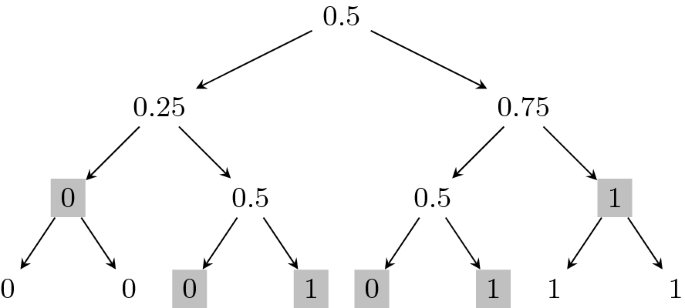
Majority Protocol Tree of depth three. The optimal score in the majority tree of depth three is 0.3750 and the corresponding stopping time is highlighted in gray.
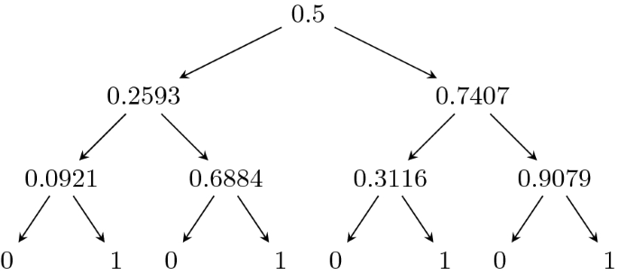
Optimal depth-3 protocol tree for \(X_0=1/2\). The optimal score is 0.2407. Observe that any stopping time achieves this score.
In the sequel, we highlight applications of Theorem 1 to protocol constructions and hardness of computation results using these estimates.
Remark 1 (Protocol Constructions)
The optimal martingales naturally translate into n-bit distributed coin-tossing and multi-faceted dice rolling protocols.
-
1.
Corollary 1: For all \(X_0\in [0,1]\), there exists an n-bit distributed bias-\(X_0\) coin-tossing protocol for n processors with the following security guarantee. Any (computationally unbounded) adversary who follows the protocol honestly and resets at most one of the processors during the execution of the protocol can change the probability of an outcome by at most \(\frac{1}{2\sqrt{n}}\sqrt{X_0(1-X_0)}\).
Remark 2 (Hardness of Computation Results)
The lower-bound on the maximum susceptibility helps demonstrate hardness of computation results. For \(X_0=1/2\), Cleve and Impagliazzo [14] proved that one encounters  with probability \(\frac{1}{5}\). In other words, their bound guarantees that the expected gap in the martingale is at least \(\frac{1}{160\sqrt{n}}\), which is significantly smaller than our bound \(\frac{1}{2\sqrt{2 n}}\). Hardness of computation results relying on [14] (and its extensions) work only for constant \(0<X_0<1\).Footnote 2 However, our lower-bound holds for all \(X_0\in [0,1]\); for example, even when \(1/\mathrm {poly} (n) \leqslant X_0 \leqslant 1-1/\mathrm {poly} (n)\). Consequently, we extend existing hardness of computation results using our more general lower-bound.
-
1.
Theorem 2 extends the fail-stop attack of [14] on 2-party bias-\(X_0\) coin-tossing protocols (in the information-theoretic commitment hybrid). For any \(X_0\in [0,1]\), a fail-stop adversary can change the probability of the final outcome of any 2-party bias-\(X_0\) coin-tossing protocol by \(\geqslant \frac{\sqrt{2}}{12\sqrt{n+1}}X_0(1-X_0)\). This result is useful to demonstrate black-box separations results.
-
2.
Corollary 2 extends the black-box separation results of [15, 16, 23] separating (appropriate restrictions of) 2-party bias-\(X_0\) coin tossing protocols from one-way functions. We illustrate a representative new result that follows as a consequence of Corollary 2. For constant \(X_0\in (0,1)\), [15, 16, 23] rely on (the extensions of) [14] to show that it is highly unlikely that there exist 2-party bias-\(X_0\) coin tossing protocols using one-way functions in a black-box manner achieving \(o(1/\sqrt{n})\) unfairness [22]. Note that when \(X_0=1/n\), there are secure 2-party coin tossing protocols with 1/2n unfairness (based on Corollary 1) even in the information-theoretic setting. Previous results cannot determine the limits to the unfairness of 2-party bias-1/n fair coin-tossing protocols that use one-way functions in a black-box manner. Our black-box separation result (refer to Corollary 2) implies that it is highly unlikely to construct bias-1/n coin using one-way functions in a black-box manner with \(< \frac{\sqrt{2}}{12\cdot n^{3/2}}\) unfairness.
-
3.
Corollary 3 and Corollary 4 extend Cleve and Impagliazzo’s [14] result on influencing discrete control processes to arbitrary \(X_0\in [0,1]\).
1.2 Prior Approaches to the General Martingale Problem
Azuma-Hoeffding inequality [6, 25] states that if  , for all \(i\in \{1,\dotsc ,n\}\), then, essentially,
  with probability 1. That is, the final information \(X_n\) remains close to the a priori information \(X_0\). However, in our problem statement, we have \(X_n\in {\{0,1\}} \). In particular, this constraint implies that the final information \(X_n\) is significantly different from the a priori information \(X_0\). So, the initial constraint “for all \(i\in \{1,\dotsc ,n\}\) we have
  ” must be violated. What is the probability of this violation?
For \(X_0=1/2\), Cleve and Impagliazzo [14] proved that there exists a round i such that  with probability 1/5. We emphasize that the round i is a random variable and not a constant. However, the definition of the “big jump” and the “probability to encounter big jumps” both are exponentially small function of \(X_0\). So, the approach of Cleve and Impagliazzo is only applicable to constant \(X_0\in (0,1)\). Recently, in an independent work, Beimel et al. [7] demonstrate an identical bound for weak martingales (that have some additional properties), which is used to model multi-party coin-tossing protocols.
For the upper-bound, on the other hand, Doob’s martingale corresponding to the majority protocol is the only known martingale for \(X_0=1/2\) with a small maximum susceptibility. In general, to achieve arbitrary \(X_0\in [0,1]\), one considers coin tossing protocols where the outcome is 1 if the total number of heads in n uniformly random coins surpasses an appropriate threshold.
2 Preliminaries
We denote the arithmetic mean of two numbers x and y as \(\text {A.M.}(x,y):= (x+y)/{2}\). The geometric mean of these two numbers is denoted by \(\text {G.M.}(x,y):= \sqrt{x\cdot y}\) and their harmonic mean is denoted by \(\text {H.M.}(x,y):= \left( \left( x^{-1}+y^{-1}\right) /2\right) ^{-1}=2xy/(x+y)\).
Martingales and Related Definitions. The conditional expectation of a random variable X with respect to an event \(\mathcal {E}\) denoted by  , is defined as
  . For a discrete random variable Y, the conditional expectation of X with respect to Y, denoted by
  , is a random variable that takes value
  with probability
  , where
  denotes the conditional expectation of X with respect to the event \(\{\omega \in \varOmega |Y(\omega )=y\}\).
Let \(\varOmega =\varOmega _1\times \varOmega _2\times \cdots \times \varOmega _n\) denote a sample space and \((E_1,E_2,\dotsc ,E_n)\) be a joint distribution defined over \(\varOmega \) such that for each \(i\in \{1,\dotsc ,n\}\), \(E_i\) is a random variable over \(\varOmega _i\). Let \(X=\{X_i\}_{i=0}^{n}\) be a sequence of random variables defined over \(\varOmega \). We say that \(X_j\) is \(E_1,\dotsc ,E_j\) measurable if there exists a function \(g_j:\varOmega _1\times \varOmega _2\times \cdots \times \varOmega _j\rightarrow \mathbb {R} \) such that \(X_j=g_j(E_1,\dotsc ,E_j)\). Let \(X=\{X_i\}_{i=0}^{n}\) be a discrete-time martingale sequence with respect to the sequence \(E=\{E_i\}_{i=1}^{n}\). This statement implies that for each \(i\in \{0,1,\dotsc ,n\}\), we have

Note that the definition of martingale implies \(X_i\) to be \(E_1,\dotsc ,E_i\) measurable for each \(i\in \{1,\dotsc ,n\}\) and \(X_0\) to be constant. In the sequel, we shall use \(\{ X=\{X_i\}_{i=0}^{n},E=\{E_i\}^n_{i=1} \}\) to denote a martingale sequence where for each \(i=1,\dotsc ,n\), \(X_i\in [0,1]\), and \(X_n\in \{0,1\}\). However, for brevity, we use \(\left( X_0,X_1,\dotsc ,X_n\right) \) to denote a martingale. Given a function \(f:\varOmega _1\times \varOmega _2\times \cdots \times \varOmega _n\rightarrow \mathbb {R}\), if we define the random variable  , for each \(i\in \{0,1,\dotsc ,n\}\), then the sequence \(Z=\{Z_i\}_{i=0}^{n}\) is a martingale with respect to \(\{E_i\}_{i=1}^{n}\). This martingale is called the Doob’s martingale.
The random variable \(\tau :\varOmega \rightarrow \{0,1,\dotsc , n\}\) is called a stopping time if for each \(k\in \{1,2,\dotsc ,n\}\), the occurrence or non-occurrence of the event \(\{\tau \leqslant k\} := \{\omega \in \varOmega | \tau (\omega )\leqslant k\}\) depends only on the values of random variables \(E_1,E_2,\dotsc ,E_k\). Equivalently, the random variable  is \(E_1,\dotsc , E_k\) measurable. Let \(\mathcal {S}(X,E)\) denote the set of all stopping time random variables over the martingale sequence \(\{ X=\{X_i\}_{i=0}^{n},E=\{E_i\}^n_{i=1} \}\). For \( \ell \in \{1,2\}\), we define the score of a martingale sequence (X, E) with respect to a stopping time \(\tau \) in the \(L_\ell \)-norm as the following quantity.

We define the max stopping time as the stopping time that maximizes the score

and the (corresponding) \(\mathrm {max}\hbox {-}\mathrm {score}\) as

Let \(A_n(x^{*})\) denote the set of all discrete time martingales \(\{X=\{X_i\}_{i=0}^n,E=\{E_i\}_{i=1}^n\}\) such that \(X_0=x^{*}\) and \(X_n \in \{0,1\}\). We define optimal score as
Representing a Martingale as a Tree. We interpret a discrete time martingale sequence \(X=\{X_i\}_{i=0}^{n}\) defined over a sample space \(\varOmega =\varOmega _1\times \cdots \times \varOmega _n\) as a tree of depth n (see Fig. 3). For \(i=0,\dotsc ,n\), any node at depth i has  children. In fact, for each i, the edge between a node at depth i and a child at depth \((i+1)\) corresponds to a possible outcome that \(E_{i+1}\) can take from the set \(\varOmega _{i+1}=\{x^{{\left( 1\right) }},\dotsc ,x^{{\left( t\right) }} \}\).
Each node v at depth i is represented by a unique path from root to v like \((e_1,e_2,\dots ,e_{i})\), which corresponds to the event \(\{\omega \in \varOmega |E_1(\omega )=e_1,\dots ,E_{i}(\omega )=e_{i}\}\). Specifically, each path from root to a leaf in this tree, represents a unique outcome in the sample space \(\varOmega \).
Any subset of nodes in a tree that has the property that none of them is an ancestor of any other, is called an anti-chain. If we use our tree-based notation to represent a node v, i.e., the sequence of edges \(e_1,\dots ,e_i\) corresponding to the path from root to v, then any prefix-free subset of nodes is an anti-chain. Any anti-chain that is not a proper subset of another anti-chain is called a maximal anti-chain. A stopping time in a martingale corresponds to a unique maximal anti-chain in the martingale tree.
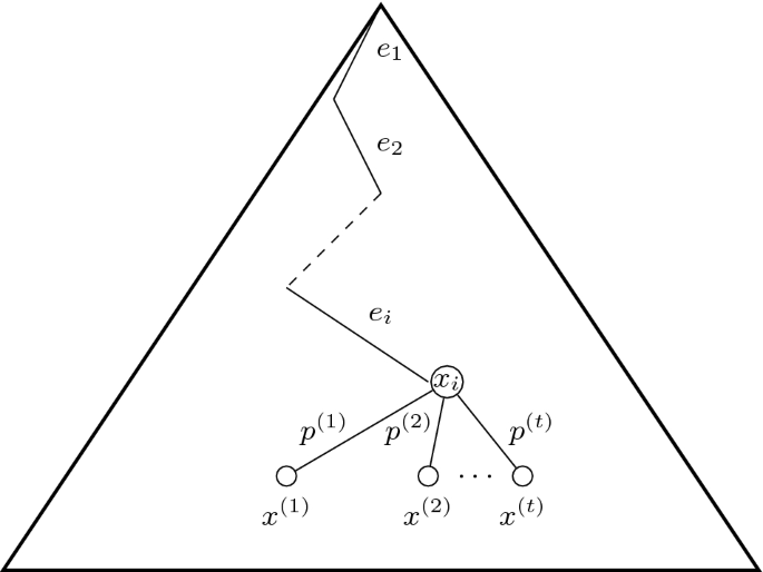
Interpreting a general martingale as a tree.
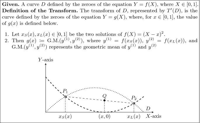
Geometric Definitions and Relations. Consider curves C and D defined by the zeroes of \(Y=f(X)\) and \(Y=g(X)\), respectively, where \(X\in [0,1]\). We restrict to curves C and D such that each one of them have exactly one intersection with \(X=x\), for any \(x\in [0,1]\). Refer to Fig. 4 for intuition. Then, we say C is above D, represented by \(C \succcurlyeq D \), if, for each \(x\in [0,1]\), we have \(f(x) \geqslant g(x)\).
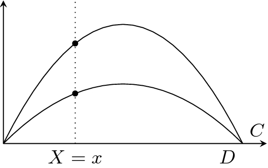
Intuition for a curve C being above another curve D, represented by \(C \succcurlyeq D \).
3 Large Gaps in Martingales: A Geometric Approach
This section presents a high-level overview of our proof strategy. In the sequel, we shall assume that we are working with discrete-time martingales \((X_0,X_1,\dotsc ,X_n)\) such that \(X_n\in {\{0,1\}} \).
Given a martingale \((X_0,\dotsc ,X_n)\), its susceptibility is represented by the following quantity

Intuitively, if a martingale has high susceptibility, then it has a stopping time such that the gap in the martingale while encountering the stopping time is large. Our objective is to characterize the least susceptibility that a martingale \((X_0,\dotsc ,X_n)\) can achieve. More formally, given n and \(X_0\), characterize

Our approach is to proceed by induction on n to exactly characterize the curve \(C_n(X)\), and our argument naturally constructs the best martingale that achieves \(C_n(X_0)\).
-
1.
We know that the base case is \(C_1(X) = 2X(1-X)\) (see Fig. 5 for this argument).
-
2.
Given the curve \(C_{n-1}(X)\), we identify a geometric transformation T (see Fig. 8) that defines the curve \(C_n(X)\) from the curve \(C_{n-1}(X)\). Section 3.1 summarizes the proof of this inductive step that crucially relies on the geometric interpretation of the problem, which is one of our primary technical contributions. Furthermore, for any \(n\geqslant 1\), there exist martingales such that its susceptibility is \(C_n(X_0)\).
-
3.
Finally, Appendix A proves that the curve \(C_n(X)\) lies above the curve \(L_n(X) := \frac{2}{\sqrt{2n-1}}X(1-X)\) and below the curve \(U_n(X) := \frac{1}{\sqrt{n}} \sqrt{X(1-X)}\).
3.1 Proof of Theorem 1
Our objective is the following.
-
1.
Given an arbitrary martingale (X, E), find the maximum stopping time in this martingale, i.e., the stopping time \(\tau _{\max }(X,E,1)\).
-
2.
For any depth n and bias \(X_0\), construct a martingale that achieves the max-score. We refer to this martingale as the optimal martingale. A priori, this martingale need not be unique. However, we shall see that for each \(X_0\), it is (essentially) a unique martingale.
We emphasize that even if we are only interested in the exact value of \(C_n(X_0)\) for \(X_0=1/2\), it is unavoidable to characterize \(C_{n-1}(X)\), for all values of \(X\in [0,1]\). Because, in a martingale \((X_0=1/2,X_1,\dotsc ,X_n)\), the value of \(X_1\) can be arbitrary. So, without a precise characterization of the value \(C_{n-1}(X_1)\), it is not evident how to calculate the value of \(C_n(X_0=1/2)\). Furthermore, understanding \(C_n(X_0)\), for all \(X_0\in [0,1]\), yields entirely new applications for our result.
Base Case of \(n=1\). For a martingale \((X_0,X_1)\) of depth \(n=1\), we have \(X_1\in {\{0,1\}} \). Thus, without loss of generality, we assume that \(E_1\) takes only two values (see Fig. 5). Then, it is easy to verify that the max-score is always equal to \(2X_0(1-X_0)\). This score is witnessed by the stopping time \(\tau =1\). So, we conclude that \(\mathrm {opt}_1(X_0,1) = C_1(X_0) = 2X_0(1-X_0)\)
Inductive Step. \(n=2\) (For Intuition). For simplicity, let us consider finite martingales, i.e., the sample space \(\varOmega _i\) of the random variable \(E_i\) is finite. Suppose that the root \(X_0=x\) in the corresponding martingale tree has t children with values \(x^{{\left( 1\right) }}, x^{{\left( 2\right) }}, \dotsc ,x^{{\left( t\right) }} \), and the probability of choosing the j-th child is \(p^{{\left( j\right) }} \), where \(j\in \{1,\dotsc ,t\}\) (see Fig. 6).
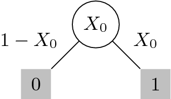
Base Case for Theorem 1. Note  . The optimal stopping time is shaded and its score is
  .
.
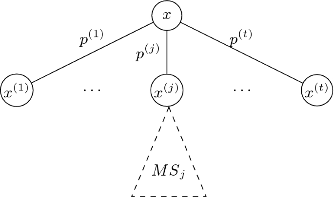
Inductive step for Theorem 1. \({MS}_j\) represents the max-score of the sub-tree of depth \(n-1\) whose rooted at \(x^{(j)}\). For simplicity, the subtree of \(x^{(j)}\) is only shown here.
Given a martingale \((X_0,X_1,X_2)\), the adversary’s objective is to find the stopping time \(\tau \) that maximizes the score  . If the adversary chooses to stop at \(\tau =0\), then the score
  , which is not a good strategy. So, for each j, the adversary chooses whether to stop at the child \(x^{{\left( j\right) }} \), or continue to a stopping time in the sub-tree rooted at \(x^{{\left( j\right) }} \). The adversary chooses the stopping time based on which of these two strategies yield a better score. If the adversary stops the martingale at child j, then the contribution of this decision to the score is
  . On the other hand, if she does not stop at child j, then the contribution from the sub-tree is guaranteed to be \(p^{{\left( j\right) }} C_1(x^{{\left( j\right) }})\). Overall, from the j-th child, an adversary obtains a score that is at least
  .
.
Let  . We represent the points \(Z^{{\left( j\right) }} =(x^{{\left( j\right) }},h^{{\left( j\right) }})\) in a two dimensional plane. Then, clearly all these points lie on the solid curve defined by
  , see Fig. 7.
Since (X, E) is a martingale, we have \(x=\sum _{j=1}^t p^{{\left( j\right) }} x^{{\left( j\right) }} \) and the adversary’s strategy for finding \(\tau _{\max }\) gives us \(\text {max-score}_1(X,E)= \sum _{j=1}^tp^{{\left( j\right) }} h^{{\left( j\right) }} \). This observation implies that the coordinate \((x,\text {max-score}_1(X,E)) = \sum _{j=1}^tp^{{\left( j\right) }} Z^{{\left( j\right) }} \). So, the point in the plane giving the adversary the maximum score for a tree of depth \(n=2\) with bias \(X_0=x\) lies in the intersection of the convex hull of the points \(Z^{{\left( 1\right) }},\dotsc ,Z^{{\left( t\right) }} \), and the line \(X=x\). Let us consider the martingale defined in Fig. 7 as a concrete example. Here \(t=4\), and the points \(Z^{{\left( 1\right) }}, Z^{{\left( 2\right) }}, Z^{{\left( 3\right) }}, Z^{{\left( 4\right) }} \) lie on  . The martingale designer specifies the probabilities \(p^{(1)}, p^{(2)}, p^{(3)}\), and \(p^{(4)}\), such that \(p^{(1)}x^{(1)} + \cdots + p^{(4)}x^{(4)}=x\). These probabilities are not represented in Fig. 7. Note that the point \(\left( p^{(1)}x^{(1)} + \dots + p^{(4)}x^{(4)}, p^{(1)}h^{(1)} +\dots + p^{(4)}h^{(4)} \right) \) representing the score of the adversary is the point \(p^{(1)}Z^{(1)}+\dots +p^{(4)}Z^{(4)}\). This point lies inside the convex hull of the points \(Z^{(1)}, \dots ,Z^{(4)}\) and on the line \(X = p^{(1)}x^{(1)} + \dots + p^{(4)}x^{(4)}=x\). The exact location depends on \(p^{(1)},\dots ,p^{(4)}\).
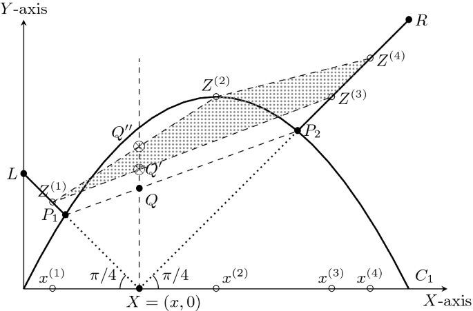
Intuitive summary of the inductive step for \(n=2\).
The point \(Q'\) is the point with minimum height. Observe that the height of the point \(Q'\) is at least the height of the point Q. So, in any martingale, the adversary shall find a stopping time that scores more than (the height of) the point Q.
On the other hand, the martingale designer’s objective is to reduce the score that an adversary can achieve. So, the martingale designer chooses \(t=2\), and the two points \(Z^{{\left( 1\right) }} =P_1\) and \(Z^{{\left( 2\right) }} =P_2\) to construct the optimum martingale. We apply this method for each \(x\in [0,1]\) to find the corresponding point Q. That is, the locus of the point Q, for \(x\in [0,1]\), yields the curve \(C_2(X)\).
We claim that the height of the point Q is the harmonic-mean of the heights of the points \(P_1\) and \(P_2\). This claim follows from elementary geometric facts. Let \(h_1\) represent the height of the point \(P_1\), and \(h_2\) represent the height of the point \(P_2\). Observe that the distance of \(x - x_S(x) = h_1\) (because the line \(\ell _1\) has slope \(\pi - \pi /4\)). Similarly, the distance of \(x_L(x)-x=h_2\) (because the line \(\ell _2\) has slope \(\pi /4\)). So, using properties of similar triangles, the height of Q turns out to be
This property inspires the definition of the geometric transformation T, see Fig. 8. Applying T on the curve \(C_1(X)\) yields the curve \(C_2(X)\) for which we have \(C_2(x) = \mathrm {opt}_2(x,1)\).
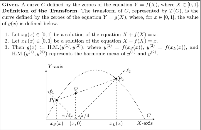
Definition of transform of a curve C, represented by T(C). The locus of the point Q (in the right figure) defines the curve T(C).
General Inductive Step. Note that a similar approach works for general \(n=d\geqslant 2\). Fix \(X_0\) and \(n=d\geqslant 2\). We assume that the adversary can compute \(C_{d-1}(X_1)\), for any \(X_1\in [0,1]\).
Suppose the root in the corresponding martingale tree has t children with values \(x^{{\left( 1\right) }}, x^{{\left( 2\right) }},\dotsc ,x^{{\left( t\right) }} \), and the probability of choosing the j-th child is \(p^{{\left( j\right) }} \) (see Fig. 6). Let \((X^{{\left( j\right) }},E^{{\left( j\right) }})\) represent the martingale associated with the sub-tree rooted at \(x^{{\left( j\right) }} \).
For any \(j\in \{1,\dotsc ,t\}\), the adversary can choose to stop at the child j. This decision will contribute  to the score with weight \(p^{{\left( j\right) }} \). On the other hand, if she continues to the subtree rooted at \(x^{{\left( j\right) }} \), she will get at least a contribution of \(\text {max-score}_1(X^{{\left( j\right) }},E^{{\left( j\right) }})\) with weight \(p^{{\left( j\right) }} \). Therefore, the adversary can obtain the following contribution to her score

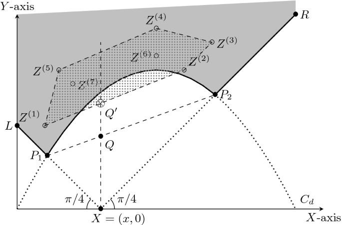
Intuitive Summary of the inductive argument. Our objective is to pick the set of points \(\{Z^{{\left( 1\right) }}, Z^{{\left( 2\right) }} \dotsc \}\) in the gray region to minimize the length of the intercept \(XQ'\) of their (lower) convex hull on the line \(X=x\). Clearly, the unique optimal solution corresponds to including both \(P_1\) and \(P_2\) in the set.
Similar to the case of \(n=2\), we define the points \(Z^{{\left( 1\right) }},\dotsc ,Z^{{\left( t\right) }} \). For \(n> 2\), however, there is one difference from the \(n=2\) case. The point \(Z^{{\left( j\right) }} \) need not lie on the solid curve, but it can lie on or above it, i.e., they lie in the gray area of Fig. 9. This phenomenon is attributable to a suboptimal martingale designer producing martingales with suboptimal scores, i.e., strictly above the solid curve. For \(n=1\), it happens to be the case that, there is (effectively) only one martingale that the martingale designer can design (the optimal tree). The adversary obtains a score that is at least the height of the point \(Q'\), which is at least the height of Q. On the other hand, the martingale designer can choose \(t=2\), and \(Z^{{\left( 1\right) }} =P_1\) and \(Z^{{\left( 2\right) }} =P_2\) to define the optimum martingale. Again, the locus of the point Q is defined by the curve \(T(C_{d-1})\).
Conclusion. So, by induction, we have proved that \(C_n(X) = T^{n-1}(C_1(X))\). Additionally, note that, during induction, in the optimum martingale, we always have  and
and  . Intuitively, the decision to stop at \(x^{{\left( j\right) }} \) or continue to the subtree rooted at \(x^{{\left( j\right) }} \) has identical consequence. So, by induction, all stopping times in the optimum martingale have score \(C_n(x)\).
Finally, Appendix A proves Lemma 1, which tightly estimates the curve \(C_n\).
4 Applications
This section discusses various consequences of Theorem 1 and other related results.
4.1 Distributed Coin-Tossing Protocol
We consider constructing distributed n-processor coin-tossing protocols where the i-th processor broadcasts her message in the i-th round. We shall study this problem in the information-theoretic setting. Our objective is to design n-party distributed coin-tossing protocols where an adversary cannot bias the distribution of the final outcome significantly.
For \(X_0=1/2\), one can consider the incredibly elegant “majority protocol” [5, 10, 13]. The i-th processor broadcasts a uniformly random bit in round i. The final outcome of the protocol is the majority of the n outcomes, and an adversary can bias the final outcome by \(\frac{1}{\sqrt{2\pi n}}\) by restarting a processor once [13].
We construct distributed n-party bias-\(X_0\) coin-tossing protocols, for any \(X_0\in [0,1]\), and our new protocol for \(X_0=1/2\) is more robust to restarting attacks than this majority protocol. Fix \(X_0\in [0,1]\) and \(n\geqslant 1\). Consider the optimal martingale \((X_0,X_1,\dotsc ,X_n)\) guaranteed by Theorem 1. The susceptibility corresponding to any stopping time is \(=C_n(X_0) \leqslant U_n(X_0) = \frac{1}{\sqrt{n}}\sqrt{X_0(1-X_0)}\). Note that one can construct an n-party coin-tossing protocol where the i-th processor broadcasts the i-th message, and the corresponding Doob’s martingale is identical to this optimal martingale. An adversary who can restart a processor once biases the outcome of this protocol by at most \(\frac{1}{2} C_n(X_0)\), this is discussed in Sect. 4.3.
Corollary 1 (Distributed Coin-tossing Protocols)
For every \(X_0\in [0,1]\) and \(n\geqslant 1\) there exists an n-party bias-\(X_0\) coin-tossing protocol such that any adversary who can restart a processor once causes the final outcome probability to deviate by \(\leqslant \frac{1}{2}C_n(X_0) \leqslant \frac{1}{2}U_n(X_0) = \frac{1}{2\sqrt{n}} \sqrt{X_0(1-X_0)}\).
For \(X_0=1/2\), our new protocol’s outcome can be changed by \(\frac{1}{4\sqrt{n}}\), which is less than the \(\frac{1}{\sqrt{2\pi n}}\) deviation of the majority protocol. However, we do not know whether there exists a computationally efficient algorithm implementing the coin-tossing protocols corresponding to the optimal martingales.
4.2 Fail-Stop Attacks on Coin-Tossing/Dice-Rolling Protocols
A two-party n-round bias-\(X_0\) coin-tossing protocol is an interactive protocol between two parties who send messages in alternate rounds, and \(X_0\) is the probability of the coin-tossing protocol’s outcome being heads. Fair computation ensures that even if one of the parties aborts during the execution of the protocol, the other party outputs a (randomized) heads/tails outcome. This requirement of guaranteed output delivery is significantly stringent, and Cleve [13] demonstrated a computationally efficient attack strategy that alters the output-distribution by O(1/n), i.e., any protocol is O(1/n) unfair. Defining fairness and constructing fair protocols for general functionalities has been a field of highly influential research [2,3,4, 8, 21, 22, 29]. This interest stems primarily from the fact that fairness is a desirable attribute for secure-computation protocols in real-world applications. However, designing fair protocol even for simple functionalities like (bias-1/2) coin-tossing is challenging both in the two-party and the multi-party setting. In the multi-party setting, several works [1, 5, 9] explore fair coin-tossing where the number of adversarial parties is a constant fraction of the total number of parties. For a small number of parties, like the two-party and the three-party setting, constructing such protocols have been extremely challenging even against computationally bounded adversaries [12, 24, 30]. These constructions (roughly) match Cleve’s O(1/n) lower-bound in the computational setting.
In the information-theoretic setting, Cleve and Impagliazzo [14] exhibited that any two-party n-round bias-1/2 coin-tossing protocol are \(\frac{1}{2560\sqrt{n}}\) unfair. In particular, their adversary is a fail-stop adversary who follows the protocol honestly except aborting prematurely. In the information-theoretic commitment-hybrid, there are two-party n-round bias-1/2 coin-tossing protocols that have \({\approx }1/\sqrt{n}\) unfairness [5, 10, 13]. This bound matches the lower-bound of \(\varOmega (1/\sqrt{n})\) by Cleve and Impagliazzo [14]. It seems that it is necessary to rely on strong computational hardness assumptions or use these primitives in a non-black box manner to beat the \(1/\sqrt{n}\) bound [7, 15, 16, 23].
We generalize the result of Cleve and Impagliazzo [14] to all 2-party n-round bias-\(X_0\) coin-tossing protocols (and improve the constants by two orders of magnitude). For \(X_0=1/2\), our fail-stop adversary changes the final outcome probability by \(\geqslant \frac{1}{24\sqrt{2}}\cdot \frac{1}{\sqrt{n+1}}\).
Theorem 2 (Fail-stop Attacks on Coin-tossing Protocols)
For any two-party n-round bias-\(X_0\) coin-tossing protocol, there exists a fail-stop adversary that changes the final outcome probability of the honest party by at least \(\frac{1}{12}C'_n(X_0)\geqslant \frac{1}{12} L'_n(X_0) := \frac{1}{12} \sqrt{\frac{2}{n+1}} X_0(1-X_0)\), where \(C'_1(X):= X(1-X)\) and \(C'_n(X):= {T}^{n-1}(C'_1(X))\).
This theorem is not a direct consequence of Theorem 1. The proof relies on an entirely new inductive argument; however, the geometric technique for this recursion is similar to the proof strategy for Theorem 1. Interested readers can refer to the full version of the paper [27] for details.
Black-Box Separation Results. Gordon and Katz [22] introduced the notion of 1/p-unfair secure computation for a fine-grained study of fair computation of functionalities. In this terminology, Theorem 2 states that \(\frac{c}{\sqrt{n+1}}X_0(1-X_0)\)-unfair computation of a bias-\(X_0\) coin is impossible for any positive constant \(c< \frac{\sqrt{2}}{12}\) and \(X_0\in [0,1]\).
Cleve and Impagliazzo’s result [14] states that \(\frac{c}{\sqrt{n}}\)-unfair secure computation of the bias-1/2 coin is impossible for any positive constant \(c< \frac{1}{2560}\). This result on the hardness of computation of fair coin-tossing was translated into black-box separations results. These results [15, 16, 23], intuitively, indicate that it is unlikely that \(\frac{c}{\sqrt{n}}\)-unfair secure computation of the bias-1/2 coin exists, for \(c< \frac{1}{2560}\), relying solely on the black-box use of one-way functions. We emphasize that there are several restrictions imposed on the protocols that these works [15, 16, 23] consider; detailing all of which is beyond the scope of this draft. Substituting the result of [14] by Theorem 2, extends the results of [15, 16, 23] to general bias-\(X_0\) coin-tossing protocols.
Corollary 2 (Informal: Black-box Separation)
For any \(X_0\in [0,1]\) and positive constant \(c< \frac{\sqrt{2}}{12}\), the existence of \(\frac{c}{\sqrt{n+1}}X_0(1-X_0)\)-unfair computation protocol for a bias-\(X_0\) coin is black-box separated from the existence of one-way functions (restricted to the classes of protocols considered by [15, 16, 23]).
4.3 Influencing Discrete Control Processes
Lichtenstein et al. [28] considered the problem of an adversary influencing the outcome of a stochastic process through mild interventions. For example, an adversary attempts to bias the outcome of a distributed n-processor coin-tossing protocol, where, in the i-th round, the processor i broadcasts her message. This model is also used to characterize randomness sources that are adversarially influenced, for example, [11, 17,18,19, 26, 31,32,33,34,35].
Consider the sample space \(\varOmega =\varOmega _1\times \varOmega _2\times \cdots \times \varOmega _n\) and a joint distribution \((E_1,\dotsc ,E_n)\) over the sample space. We have a function \(f:\varOmega \rightarrow {\{0,1\}} \) such that  . This function represents the protocol that determines the final outcome from the public transcript. The filtration, at time-step i, reveals the value of the random variable \(E_i\) to the adversary. We consider the corresponding Doob’s martingale \((X_0,X_1,\dotsc ,X_n)\). Intuitively, \(X_i\) represents the probability of \(f(E_1,\dotsc ,E_n)=1\) conditioned on the revealed values \((E_1=e_1,\dotsc ,E_i=e_i)\). The adversary is allowed to intervene only once. She can choose to intervene at time-step i, reject the current sample \(E_i=e_i\), and substitute it with a fresh sample from \(E_i\). This intervention is identical to restarting the i-th processor if the adversary does not like her message. Note that this intervention changes the final outcome by
We shall use a stopping time \(\tau \) to represent the time-step where an adversary decides to intervene. However, for some \((E_1=e_1,\dotsc ,E_n=e_n)\) the adversary may not choose to intervene. Consequently, we consider stopping times \(\tau :\varOmega \rightarrow \{1,\dotsc ,n,\infty \}\), where the stopping time being \(\infty \) corresponds to the event that the adversary did not choose to intervene. In the Doob martingale discussed above, as a direct consequence of Theorem 1, there exists a stopping time \(\tau ^*\) with susceptibility \(\geqslant C_n(X_0)\). Note that susceptibility measures the expected (unsigned) magnitude of the deviation, if an adversary intervenes at \(\tau ^*\). Some of these contributions to susceptibility shall increase the probability of the final outcome being 1, and the remaining shall decrease the probability of the final outcome being 1. By an averaging argument, there exists a stopping time \(\tau :\varOmega \rightarrow \{1,\dotsc ,n,\infty \}\) that biases the outcome of f by at least \(\geqslant \frac{1}{2} C_n(X_0)\), whence the following corollary.
Corollary 3 (Influencing Discrete Control Processes)
Let \(\varOmega _1,\dotsc ,\varOmega _n\) be arbitrary sets, and \((E_1,\dotsc ,E_n)\) be a joint distribution over the set \(\varOmega := \varOmega _1\times \cdots \times \varOmega _n\). Let \(f:\varOmega \rightarrow {\{0,1\}} \) be a function such that  . Then, there exists an adversarial strategy of intervening once to bias the probability of the outcome away from \(X_0\) by \(\geqslant \frac{1}{2}C_n(X_0) \geqslant \frac{1}{2}L_n(X_0) =\frac{1}{\sqrt{2n-1}}X_0(1-X_0)\).
The previous result of [14] applies only to \(X_0=1/2\) and they ensure a deviation of \(1/320\sqrt{n}\). For \(X_0=1/2\), our result ensures a deviation of (roughly) \(1/4\sqrt{2n} \approx 1/5.66\sqrt{n}\).
Influencing Multi-faceted Dice-Rolls. Corollary 3 generalizes to the setting where \(f:\varOmega \rightarrow \{0,1,\dotsc ,\omega -1\}\), i.e., the function f outputs an arbitrary \(\omega \)-faceted dice roll. In fact, we quantify the deviation in the probability of any subset \(S\subseteq \{0,1,\dotsc ,\omega -1\}\) of outcomes caused by an adversary intervening once.
Corollary 4 (Influencing Multi-faceted Dice-Rolls)
Let \(\varOmega _1,\dotsc ,\varOmega _n\) be arbitrary sets, and \((E_1,\dotsc ,E_n)\) be a joint distribution over the set \(\varOmega := \varOmega _1\times \cdots \times \varOmega _n\). Let \(f:\varOmega \rightarrow \{0,1,\dotsc ,\omega -1\}\) be a function with \(\omega \geqslant 2\) outcomes, \(S\subseteq \{0,1,\dotsc ,\omega -1\}\) be any subset of outcomes, and  . Then, there exists an adversarial strategy of intervening once to bias the probability of the outcome being in S away from \(X_0\) by \(\geqslant \frac{1}{2}C_n(X_0) \geqslant \frac{1}{2}L_n(X_0) =\frac{1}{\sqrt{2n-1}}X_0(1-X_0)\).
Corollary 3 and Corollary 4 are equivalent to each other. Clearly Corollary 3 is a special case of Corollary 4. Corollary 4, in turn, follows from Corollary 3 by considering “\(f(E_1,\dotsc ,E_n)\in S\)” as the interesting event for the martingale. We state these two results separately for conceptual clarity and ease of comparison with the prior work.
4.4 \(L_2\) Gaps and Their Tightness
Finally, to demonstrate the versatility of our geometric approach, we measure large \(L_2\)-norm gaps in martingales.
Theorem 3
Let \((X_0,X_1,\dotsc ,X_n)\) be a discrete-time martingale such that \(X_n\in \{0,1\}\). Then, the following bound holds.

Furthermore, for all \(n\geqslant 1\) and \(X_0\in [0,1]\), there exists a martingale \((X_0,\dotsc ,X_n)\) such that for any stopping time \(\tau \), it has  .
.
We provide a high-level overview of the proof in Appendix B.
Note that, for any martingale \((X_0,\dotsc ,X_n)\) with \(X_n\in {\{0,1\}} \), we have  . Therefore, by an averaging argument, there exists a round i such that
  . Theorem 3 proves the existence of a martingale that achieves the lower-bound even for non-constant stopping times.
This result provides an alternate technique to obtain the upper-bound to \(C_n(X)\) in Lemma 1.
Notes
- 1.
For the introduction, we do not explicitly mention the underlying filtration for brevity. The proofs, however, clearly mention the associated filtrations.
- 2.
Cleve and Impagliazzo set their problem as an optimization problem that trades off two conflicting objective functions. These objective functions have exponential dependence on \(X_0(1-X_0)\). Consequently, if \(X_0=1/\mathrm {poly} (n)\) or \(X_0=1-1/\mathrm {poly} (n)\), then their lower bounds are extremely weak.
References
Alon, B., Omri, E.: Almost-optimally fair multiparty coin-tossing with nearly three-quarters malicious. In: Hirt, M., Smith, A. (eds.) TCC 2016. LNCS, vol. 9985, pp. 307–335. Springer, Heidelberg (2016). https://doi.org/10.1007/978-3-662-53641-4_13
Asharov, G.: Towards characterizing complete fairness in secure two-party computation. In: Lindell, Y. (ed.) TCC 2014. LNCS, vol. 8349, pp. 291–316. Springer, Heidelberg (2014). https://doi.org/10.1007/978-3-642-54242-8_13
Asharov, G., Beimel, A., Makriyannis, N., Omri, E.: Complete characterization of fairness in secure two-party computation of boolean functions. In: Dodis, Y., Nielsen, J.B. (eds.) TCC 2015. LNCS, vol. 9014, pp. 199–228. Springer, Heidelberg (2015). https://doi.org/10.1007/978-3-662-46494-6_10
Asharov, G., Lindell, Y., Rabin, T.: A full characterization of functions that imply fair coin tossing and ramifications to fairness. In: Sahai, A. (ed.) TCC 2013. LNCS, vol. 7785, pp. 243–262. Springer, Heidelberg (2013). https://doi.org/10.1007/978-3-642-36594-2_14
Awerbuch, B., Blum, M., Chor, B., Goldwasser, S., Micali, S.: How to implement Bracha’s O(log n) byzantine agreement algorithm. Unpublished manuscript (1985)
Azuma, K.: Weighted sums of certain dependent random variables. Tohoku Math. J. (2) 19(3), 357–367 (1967). https://doi.org/10.2748/tmj/1178243286
Beimel, A., Haitner, I., Makriyannis, N., Omri, E.: Tighter bounds on multi-party coin flipping via augmented weak martingales and differentially private sampling. In: 2018 IEEE 59th Annual Symposium on Foundations of Computer Science (FOCS), pp. 838–849. IEEE (2018)
Beimel, A., Lindell, Y., Omri, E., Orlov, I.: 1/p-secure multiparty computation without honest majority and the best of both worlds. In: Rogaway, P. (ed.) CRYPTO 2011. LNCS, vol. 6841, pp. 277–296. Springer, Heidelberg (2011). https://doi.org/10.1007/978-3-642-22792-9_16
Beimel, A., Omri, E., Orlov, I.: Protocols for multiparty coin toss with dishonest majority. In: Rabin, T. (ed.) CRYPTO 2010. LNCS, vol. 6223, pp. 538–557. Springer, Heidelberg (2010). https://doi.org/10.1007/978-3-642-14623-7_29
Blum, M.: How to exchange (secret) keys (extended abstract). In: 15th Annual ACM Symposium on Theory of Computing, Boston, MA, USA, 25–27 April 1983, pp. 440–447. ACM Press (1983). https://doi.org/10.1145/800061.808775
Bosley, C., Dodis, Y.: Does privacy require true randomness? In: Vadhan, S.P. (ed.) TCC 2007. LNCS, vol. 4392, pp. 1–20. Springer, Heidelberg (2007). https://doi.org/10.1007/978-3-540-70936-7_1
Buchbinder, N., Haitner, I., Levi, N., Tsfadia, E.: Fair coin flipping: tighter analysis and the many-party case. In: Klein, P.N. (ed.) 28th Annual ACM-SIAM Symposium on Discrete Algorithms, Barcelona, Spain, 16–19 January 2017, pp. 2580–2600. ACM-SIAM (2017). https://doi.org/10.1137/1.9781611974782.170
Cleve, R.: Limits on the security of coin flips when half the processors are faulty (extended abstract). In: 18th Annual ACM Symposium on Theory of Computing, Berkeley, CA, USA, 28–30 May 1986, pp. 364–369. ACM Press (1986). https://doi.org/10.1145/12130.12168
Cleve, R., Impagliazzo, R.: Martingales, collective coin flipping and discrete control processes (extended abstract) (1993)
Dachman-Soled, D., Lindell, Y., Mahmoody, M., Malkin, T.: On the black-box complexity of optimally-fair coin tossing. In: Ishai, Y. (ed.) TCC 2011. LNCS, vol. 6597, pp. 450–467. Springer, Heidelberg (2011). https://doi.org/10.1007/978-3-642-19571-6_27
Dachman-Soled, D., Mahmoody, M., Malkin, T.: Can optimally-fair coin tossing be based on one-way functions? In: Lindell, Y. (ed.) TCC 2014. LNCS, vol. 8349, pp. 217–239. Springer, Heidelberg (2014). https://doi.org/10.1007/978-3-642-54242-8_10
Dodis, Y., Ong, S.J., Prabhakaran, M., Sahai, A.: On the (im)possibility of cryptography with imperfect randomness. In: 45th Annual Symposium on Foundations of Computer Science, Rome, Italy, 17–19 October 2004, pp. 196–205. IEEE Computer Society Press (2004). https://doi.org/10.1109/FOCS.2004.44
Dodis, Y., Pietrzak, K., Przydatek, B.: Separating sources for encryption and secret sharing. In: Halevi, S., Rabin, T. (eds.) TCC 2006. LNCS, vol. 3876, pp. 601–616. Springer, Heidelberg (2006). https://doi.org/10.1007/11681878_31
Dodis, Y., Spencer, J.: On the (non)universality of the one-time pad. In: 43rd Annual Symposium on Foundations of Computer Science, Vancouver, BC, Canada, 16–19 November 2002, pp. 376–387. IEEE Computer Society Press (2002). https://doi.org/10.1109/SFCS.2002.1181962
Goldwasser, S., Kalai, Y.T., Park, S.: Adaptively secure coin-flipping, revisited. In: Halldórsson, M.M., Iwama, K., Kobayashi, N., Speckmann, B. (eds.) ICALP 2015. LNCS, vol. 9135, pp. 663–674. Springer, Heidelberg (2015). https://doi.org/10.1007/978-3-662-47666-6_53
Gordon, S.D., Hazay, C., Katz, J., Lindell, Y.: Complete fairness in secure two-party computation. In: Ladner, R.E., Dwork, C. (eds.) 40th Annual ACM Symposium on Theory of Computing, Victoria, BC, Canada, 17–20 May 2008, pp. 413–422. ACM Press (2008). https://doi.org/10.1145/1374376.1374436
Gordon, S.D., Katz, J.: Partial fairness in secure two-party computation. In: Gilbert, H. (ed.) EUROCRYPT 2010. LNCS, vol. 6110, pp. 157–176. Springer, Heidelberg (2010). https://doi.org/10.1007/978-3-642-13190-5_8
Haitner, I., Omri, E., Zarosim, H.: Limits on the usefulness of random oracles. In: Sahai, A. (ed.) TCC 2013. LNCS, vol. 7785, pp. 437–456. Springer, Heidelberg (2013). https://doi.org/10.1007/978-3-642-36594-2_25
Haitner, I., Tsfadia, E.: An almost-optimally fair three-party coin-flipping protocol. In: Shmoys, D.B. (ed.) 46th Annual ACM Symposium on Theory of Computing, New York, NY, USA, 31 May–3 June 2014, pp. 408–416. ACM Press (2014). https://doi.org/10.1145/2591796.2591842
Hoeffding, W.: Probability inequalities for sums of bounded random variables. J. Am. Stat. Assoc. 58(301), 13–30 (1963). https://doi.org/10.1080/01621459.1963.10500830
Kenyon, C., Rabani, Y., Sinclair, A.: Biased random walks, Lyapunov functions, and stochastic analysis of best fit bin packing (preliminary version). In: Tardos, É. (ed.) 7th Annual ACM-SIAM Symposium on Discrete Algorithms, Atlanta, Georgia, USA, 28–30 January 1996, pp. 351–358. ACM-SIAM (1996)
Khorasgani, H.A., Maji, H., Mukherjee, T.: Estimating gaps in martingales and applications to coin-tossing: constructions and hardness. Cryptology ePrint Archive, Report 2019/774 (2019). https://eprint.iacr.org/2019/774
Lichtenstein, D., Linial, N., Saks, M.: Some extremal problems arising from discrete control processes. Combinatorica 9(3), 269–287 (1989)
Makriyannis, N.: On the classification of finite boolean functions up to fairness. In: Abdalla, M., De Prisco, R. (eds.) SCN 2014. LNCS, vol. 8642, pp. 135–154. Springer, Cham (2014). https://doi.org/10.1007/978-3-319-10879-7_9
Moran, T., Naor, M., Segev, G.: An optimally fair coin toss. In: Reingold, O. (ed.) TCC 2009. LNCS, vol. 5444, pp. 1–18. Springer, Heidelberg (2009). https://doi.org/10.1007/978-3-642-00457-5_1
Nisan, N.: Extracting randomness: how and why-a survey. In: CCC, p. 44. IEEE (1996)
Nisan, N., Ta-Shma, A.: Extracting randomness: a survey and new constructions. J. Comput. Syst. Sci. 58(1), 148–173 (1999)
Srinivasan, A., Zuckerman, D.: Computing with very weak random sources. In: 35th Annual Symposium on Foundations of Computer Science, Santa Fe, NM, USA, 20–22 November 1994, pp. 264–275. IEEE Computer Society Press (1994). https://doi.org/10.1109/SFCS.1994.365688
Trevisan, L., Vadhan, S.P.: Extracting randomness from samplable distributions. In: 41st Annual Symposium on Foundations of Computer Science, Redondo Beach, CA, USA, 12–14 November 2000, pp. 32–42. IEEE Computer Society Press (2000). https://doi.org/10.1109/SFCS.2000.892063
Zuckerman, D.: Simulating BPP using a general weak random source. Algorithmica 16(4–5), 367–391 (1996)
Author information
Authors and Affiliations
Corresponding author
Editor information
Editors and Affiliations
Appendices
A Proof of Lemma 1
In this appendix, we summarize a high-level argument proving Lemma 1. For a complete proof, readers are encouraged to read the full version of this paper [27].
Recall that we defined \(L_n(X) = \frac{2}{\sqrt{2n-1}} X(1-X)\) and \(U_n(X) = \frac{1}{\sqrt{n}}\)\(\sqrt{X(1-X)}\). Our objective is to inductively prove that \(U_n \succcurlyeq C_n \succcurlyeq L_n\), for \(n\geqslant 1\).
A crucial property of convex upwards curves that we use in our proof is the following. Suppose we have \(C\succcurlyeq D\), where C and D are two convex upwards curves above the axis \(Y=0\) defined in the domain \(X\in [0,1]\) containing the points (0, 0) and (1, 0). Then, we have \(T(C)\succcurlyeq T(D)\). This result is formalized in Lemma 2 and Fig. 10 summarizes the intuition of its proof.
Lemma 2
Let C and D be concave downward curves in the domain \(X\in [0,1]\), and both curves C and D are above the axis \(Y=0\) and contain the points (0, 0) and (1, 0). Let C and D be curves such that \(C\succcurlyeq D\) in the domain \(X\in [0,1]\), then we have \(T(C)\succcurlyeq T(D)\).
Summary of the intuition underlying the proof of Lemma 2.
Base Case of \(n=1\). Since, \(C_1(X)=L_1(X) = 2X(1-X)\), it is obvious that \(C_1\succcurlyeq L_1\). Moreover, we know that \(U_1(X) = \sqrt{X(1-X)}\). It is easy to verify that \(U_1(X) \geqslant C_1(X)\) for all \(X\in [0,1]\) which is equivalent to \(U_1 \succcurlyeq C_1\).
Inductive Argument. Figure 11 pictorially summarizes the intuition underlying our inductive argument.

The outline of the inductive proof demonstrating that if the curves \(U_i\) and \(L_i\) sandwich the curve \(C_i\), then the curves \(U_{i+1}\) and \(L_{i+1}\) sandwich the curve \(C_{i+1}\). Recall that the notation “\(A \succcurlyeq B\)” implies that the curve A lies on-or-above the curve B.
Suppose we inductively have \(U_n\succcurlyeq C_n\succcurlyeq L_n\). Then, we have \(T(U_n)\succcurlyeq T(C_n)\succcurlyeq T(L_n)\) (by Lemma 2). Note that \(C_{n+1}=T(C_n)\). In the full version of the paper [27], we prove that \(T(L_n)\succcurlyeq L_{n+1}\), and \(U_{n+1}\succcurlyeq T(U_n)\). Consequently, it follows that \(U_{n+1}\succcurlyeq C_{n+1}\succcurlyeq L_{n+1}\).
B Large \(L_2\)-Gaps in Martingale: Proof of Theorem 3
In Sect. 3 we measured the gaps in martingales using the \(L_1\)-norm. In this section, we extend this analysis to gaps in martingales using the \(L_2\)-norm. To begin, let us fix \(X_0\) and n. We change the definition of susceptibility to

Our objective is to characterize the martingale that is least susceptible

We shall proceed by induction on n and prove that \(D_n(X_0) = \frac{1}{n}X_0(1-X_0)\). Furthermore, there are martingales such that any stopping time \(\tau \) has \(D_n(X_0)\) susceptibility.
Base Case \(n=1\). Note that in this case (see Fig. 5) the optimal stopping time is \(\tau =1\).
General Inductive Step. Let us fix \(X_0=x\) and \(n=d\geqslant 2\). We proceed analogous to the argument in Sect. 3.1. The adversary can either decide to stop at the child j (see Fig. 6 for reference) or continue to the subtree rooted at it to find a better stopping time.
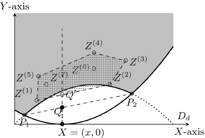
Intuitive Summary of the inductive argument. Our objective is to pick the set of points \(\{Z^{{\left( 1\right) }},Z^{{\left( 2\right) }} \dotsc \}\) in the gray region to minimize the length of the intercept \(XQ'\) of their (lower) convex hull on the line \(X=x\). Clearly, the unique optimal solution corresponds to including both \(P_1\) and \(P_2\) in this set.
Overall, the adversary gets the following contribution from the j-th child
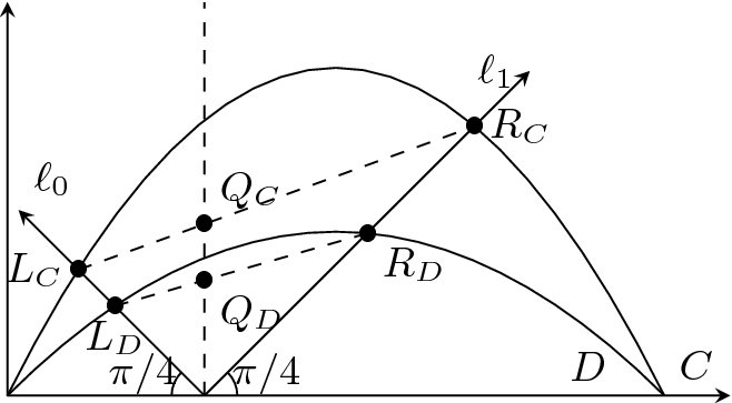
Definition of transform of a curve D, represented by \(T'(D)\). The locus of the point Q (in the right figure) defines the curve \(T'(D)\).
The adversary obtains a score that is at least the height of Q in Fig. 12. Furthermore, a martingale designer can choose \(t=2\), and \(Z^{{\left( 1\right) }} =P_1\) and \(Z^{{\left( 2\right) }} =P_2\) to define the optimal martingale. Similar to Theorem 1, the scores corresponding to all possible stopping times in the optimal martingale are identical.
One can argue that the height of Q is the geometric-mean of the heights of \(P_1\) and \(P_2\). This observation defines the geometric transformation \(T'\) in Fig. 13. For this transformation, we demonstrate that \(D_n(X_0)=\frac{1}{n}X_0(1-X_0)\) is the solution to the recursion \(D_n = {T'}^{n-1}(D_1)\).
Remark 3
It might seem curious that the upper-bound \(U_n\) happens to be the square-root of the curve \(D_n\). This occurrence is not a coincidence. We can prove that the curve \(\sqrt{D_n}\) is an upper-bound to the curve \(C_n\) (for details, refer to the full version of the paper [27]).
Rights and permissions
Copyright information
© 2019 International Association for Cryptologic Research
About this paper

Cite this paper
Khorasgani, H.A., Maji, H.K., Mukherjee, T. (2019). Estimating Gaps in Martingales and Applications to Coin-Tossing: Constructions and Hardness. In: Hofheinz, D., Rosen, A. (eds) Theory of Cryptography. TCC 2019. Lecture Notes in Computer Science(), vol 11892. Springer, Cham. https://doi.org/10.1007/978-3-030-36033-7_13
Download citation
DOI: https://doi.org/10.1007/978-3-030-36033-7_13
Published:
Publisher Name: Springer, Cham
Print ISBN: 978-3-030-36032-0
Online ISBN: 978-3-030-36033-7
eBook Packages: Computer ScienceComputer Science (R0)