Location via proxy:   [ UP ]  
[Report a bug]   [Manage cookies]                
  • Open Access

Nonergodic Delocalized States for Efficient Population Transfer within a Narrow Band of the Energy Landscape

Vadim N. Smelyanskiy, Kostyantyn Kechedzhi, Sergio Boixo, Sergei V. Isakov, Hartmut Neven, and Boris Altshuler
Phys. Rev. X 10, 011017 – Published 24 January 2020

Abstract

We address the long-standing problem of the structure of the low-energy eigenstates and long-time coherent dynamics in quantum spin-glass models. Below the spin-glass freezing transition, the energy landscape of the spin system is characterized by a proliferation of local minima where classical dynamics gets trapped. A theoretical description of quantum dynamics in this regime is challenging due to the complex nature of the distribution of the tunneling matrix elements between the local minima of the energy landscape. We study the transverse-field-induced quantum dynamics of the following “impurity band” (IB) spin model: zero energy of all spin configurations except for a small fraction of spin configurations (“marked states”) that form a narrow band at a large negative energy. At a zero transverse field, the IB model demonstrates the freezing transition at inverse temperature βf1 characterized by a nonzero value of the Edwards-Anderson order parameter. At a finite transverse field, the low-energy dynamics can be described by the effective down-folded Hamiltonian that acts in the Hilbert subspace involving only the marked states. We obtain in an explicit form the heavy-tailed probability distribution of the off-diagonal matrix elements of the down-folded Hamiltonian. This Hamiltonian is dense and belongs to the class of preferred basis Levy matrices. Analytically solving nonlinear cavity equations for the ensemble of down-folded Hamiltonians allows us to describe the statistical properties of the eigenstates. In a broad interval of transverse fields, they are nonergodic, albeit extended. It means that the band of marked states splits into a set of narrow minibands. Accordingly, the quantum evolution that starts from a particular marked state leads to a linear combination of the states belonging to a particular miniband. An analytical description of this qualitatively new type of quantum dynamics is a key result of our paper. Based on our analysis, we propose the population transfer (PT) algorithm: The quantum evolution under constant transverse field B starts at a low-energy spin configuration and ends up in a superposition of Ω spin configurations inside a narrow energy window. This algorithm crucially relies on the nonergodic nature of delocalized low-energy eigenstates. In the considered model, the run-time of the best classical algorithm (exhaustive search) is tcl=2n/Ω. For nB1, the typical run-time of the quantum PT algorithm tclen/(2B2) scales with n and Ω as that of Grover’s quantum search, except for the small correction to the exponent. Unlike the Hamiltonians proposed for analog quantum unstructured search algorithms, the model we consider is nonintegrable and the transverse field delocalizes the marked states. As a result, our PT protocol does not require fine-tuning of the transverse field and may be initialized in a computational basis state. We find that the run-times of the PT algorithm are distributed according to the alpha-stable Levy law with tail index 1. We argue that our approach can be applied to study the PT protocol in other transverse-field spin-glass models, with a potential quantum advantage over classical algorithms.

  • Figure
  • Figure
  • Figure
  • Figure
  • Figure
  • Figure
  • Figure
21 More
  • Received 28 May 2018
  • Revised 20 August 2019

DOI:https://doi.org/10.1103/PhysRevX.10.011017

Published by the American Physical Society under the terms of the Creative Commons Attribution 4.0 International license. Further distribution of this work must maintain attribution to the author(s) and the published article’s title, journal citation, and DOI.

Published by the American Physical Society

Physics Subject Headings (PhySH)

Quantum Information, Science & TechnologyCondensed Matter, Materials & Applied Physics

Authors & Affiliations

Vadim N. Smelyanskiy1,*, Kostyantyn Kechedzhi1,2,3, Sergio Boixo1, Sergei V. Isakov4, Hartmut Neven1, and Boris Altshuler5

  • 1Google, Venice, California 90291, USA
  • 2QuAIL, NASA Ames Research Center, Moffett Field, California 94035, USA
  • 3University Space Research Association, 615 National Avenue, Mountain View, California 94043, USA
  • 4Google, 8002 Zurich, Switzerland
  • 5Physics Department, Columbia University, 538 West 120th Street, New York, New York 10027, USA

  • *Corresponding author. smelyan@google.com

Popular Summary

Computational search and optimization problems are key applications of quantum computers. New insight into how efficient quantum algorithms are at solving these problems can be gained by analyzing the dynamics of quantum extensions of closely related classical spin-glass models, which allow for an analytical description of their statistical mechanics and, in limited cases, classical dynamics. We report the first analytical treatment of quantum dynamics of a model of this type and propose a protocol for the efficient search of low-energy configuration space of spin glasses.

The key technical progress of our work is the derivation of an effective low-energy Hamiltonian, which describes quantum dynamics of the model within a subspace of states with energies within a narrow band. Our derivation reduces the original spin Hamiltonian to a model of random matrix theory of exponentially smaller dimension, specified by a probability distribution of matrix elements. Within this framework, we calculate the statistics of many-body relaxation rates and demonstrate that the run-time of our “population transfer protocol” is asymptotically optimal for the impurity band model, corresponding to the multitarget Grover’s algorithm for unstructured database search.

Extensions of our analysis to a wider range of search and optimization problems present an exciting new field of research with the potential for computational speedups.
Key Image

Article Text

Click to Expand

References

Click to Expand
Issue

Vol. 10, Iss. 1 — January - March 2020

Subject Areas
Reuse & Permissions
Author publication services for translation and copyediting assistance advertisement

Authorization Required


×

Images

  • Figure 1
    Figure 1

    Cartoon of the level diagram. Horizontal blue lines depict the energy levels B(n2m) of the driver Hamiltonian HD in Eq. (1) separated by 2B. A narrow impurity band of width WB is marked in light green. The sequence of short black lines depicts the energies of marked states E(zi). Dashed lines depict the elementary path to the leading-order perturbation theory in B for the tunneling matrix element cij(E) given in Eq. (19). In this paper, we focus on the case of relatively large transverse fields B>1 so that the IB energies lie above the ground state of the total Hamiltonian (1) that corresponds to nearly all qubits polarized in the x direction.

    Reuse & Permissions
  • Figure 2
    Figure 2

    Colored lines show the dependence of the rescaled logarithm of the coupling coefficient n1logc2(E,d) [Eq. (23)] on the rescaled Hamming distance d/n for n=400. The energy E is set to the value E(0)nB2 that reflects the overall shift of the impurity band due to the transverse field [cf. Eqs. (36) and (37)]. Different colors correspond to different values of the transverse field B=1.93 (red), 1.43 (blue), 1.11 (green), 1.01 (brown), 0.99 (purple), and 0.95 (gray). The scale along the y axis suggests that c(E(0),d) scales exponentially with n for d/n=O(n0). The inset shows the leading-order factor in the d dependence of the coupling coefficient for B>|E|/n [cf. Eq. (33)]. Black dots show the boundaries d=n/2m0,n/2+m0 of the region of the oscillatory behavior of c(E,d) with d given by the WKB theory [Eq. (32)] (see Appendix pp2 for details).

    Reuse & Permissions
  • Figure 3
    Figure 3

    The black line shows the plot of 2u(m) (31) vs m between the interval boundaries ±m=L=(n+1)/2. The horizontal dashed-dotted blue line depicts the region of oscillatory behavior of Gm,n/2(E) with m for a given E described by the WKB solution (33) [see also Eq. (b5) in Appendix pp2] and shown in Fig. 4. The boundaries of this region are the turning points m=±m0(E) given by Eq. (32) and depicted with blue dots. The regions of m[m0(E),L][L,m0(E)] correspond to the exponential growth of Gm,n/2(E) with m (or decrease with d=n/2m). The WKB solution for the right region is given in Eq. (b10).

    Reuse & Permissions
  • Figure 4
    Figure 4

    The blue curve shows the d dependence of the (rescaled) coupling coefficients c(E,d) computed from the exact expression (23) with n=224 and E=226.15. We denote the binomial coefficient as (nd)Cdn. The transverse field is B=1.459. For this value of B, the impurity band levels E(zj) lie approximately in the middle of the interval between the p=34th and p=35th excited energy levels B(n2p) of the driver Hamiltonian. Red points depict the d dependence of the same rescaled coefficients c(E,d) given by Gn/2d,n/2exp(nθ) and determined by the asymptotic WKB expressions given in Appendix pp2 [see Eqs. (b10) and (b13)]. Dashed lines indicate the boundaries of the oscillatory behavior of the WKB solution [Eq. (b9)]. The inset shows the plot for the exponential d dependence of the rescaled coupling coefficient c(E,d) in the region of its monotonic behavior d[1,n/2m0(E)] [cf. Eqs. (b13) and (29)]. The solid blue line corresponds to the exact expression (23), while the approximate WKB solution is shown with red points.

    Reuse & Permissions
  • Figure 5
    Figure 5

    Plots of the WKB phase ϕdϕ(E,d) of the oscillations of the coupling coefficient c(E,d) with the Hamming distance d for a number of qubits n=1000. Both axes are rescaled by n. The phase is plotted relative to its value at d=n/2. We set the energy E=E(0), where E(0)nB2 reflects the overall shift of the impurity band due to the transverse field [cf. Eqs. (36) and (37)]. Different color curves correspond to different values of B>|E|/n with B=1.1 (brown), B=1.2 (orange), B=1.5 (red), B=2.1 (green), B=3.2 (blue), and B=10 (black). Each curve varies in its own range n/2d[m0,m0], where m0 is given in Eq. (32) and determines the region of oscillatory behavior of the coupling coefficients (see Appendix pp2 for details). For B1, the region of oscillatory behavior shrinks to a point dn/2. In the limit of large values of B1, this behavior occupies almost the entire range d[0,n].

    Reuse & Permissions
  • Figure 6
    Figure 6

    Solid lines show the dependence on the transverse field B of the eigenvalues Eβ of the nonlinear eigenvalue problem with Hamiltonian H(E) for the case of n=50 and M=2. The plot shows the repeated avoided crossing between the two systems of eigenvalues. One system (colored lines) corresponds to the eigenvalues of the transverse-field (driver) Hamiltonian HD=Bk=0nσxk in the limit Hcl0. The second system of eigenvalues corresponds to the energies of the two marked states in the limit B0. The splitting of the eigenvalues is exponentially small in n and not resolved in the plot. The asymptotic expressions (36) and (37) for the two eigenvalues E1,2(0)=E(0) neglecting the tunneling splitting and setting E(zj)=n for all j[1,M] are shown with a dashed gray line.

    Reuse & Permissions
  • Figure 7
    Figure 7

    The solid red line shows the dependence of the total weight Q vs transverse field B for n=40. Vertical black and blue lines, respectively, depict the locations of p-even and p-odd resonances B=Bp defined in the text. The total weight Q undergoes sharp decreases in the vicinity of even resonances. For p<5, the resonance regions are so narrow that dips in Q are not seen. The width of the regions grows steeply with p.

    Reuse & Permissions
  • Figure 8
    Figure 8

    Plot of the maximum value of the transverse field at midresonance point Bmax as a function of n. We define Bmax=(Bp+Bp+1)/2, where B,pn/(n2p) satisfies the equation E(0)=B,k(n2p) and the integer p is equal to its maximum possible value p=pmax for which the weight factor Q=Q((Bp+Bp+1)/2)0.98.

    Reuse & Permissions
  • Figure 9
    Figure 9

    Red points show the empirical probability distribution Mj(d) vs d with Mj(d)=j=1Mδ(dijd). Here, dij is a matrix of Hamming distances dij between the set of M randomly chosen n-bit strings (marked states), and i is a randomly chosen marked state. The distribution corresponds to M=107 and n=60. Black stars connected by a black line show the samples md from multinomial distribution with mean values Mj(d)=Mpd, where pd is binomial distribution (49).

    Reuse & Permissions
  • Figure 10
    Figure 10

    The inverse participation ratio I2=i|i|ψβ|4 as a function of the average classical (at a vanishing transverse field) energy level spacing δε in units of the typical coupling Vtyp for different numbers M of states in the impurity band. We see that for δε/Vtyp1 the eigenstates become localized and I21 independent of M, indicative of eigenstates localized on single bit string each.

    Reuse & Permissions
  • Figure 11
    Figure 11

    The rescaled inverse participation ratio I2M/3 as a function of the rescaled impurity band width W/(MVtyp) for different numbers M of states in the impurity band. We see that in the ergodic regime, W/(MVtyp)1, we have I2M/3=1, corresponding to the orthogonal Porter-Thomas distribution of states in the impurity band. The inset shows the numerical probability distribution of normalized probabilities Mp for an eigenstate over computational states z in the ergodic regime in black and the analytical orthogonal Porter-Thomas distribution in red. Qualitative arguments in Sec. 8 suggest that in the nonergodic delocalized regime I2M/3[W/(MVtyp)]2. The black line is proportional to [W/(MVtyp)]2, and we see that I2M/3 aligns with this quantity as long as we do not enter the localized regime δε/Vtyp1; see Fig. 10.

    Reuse & Permissions
  • Figure 12
    Figure 12

    The multifractal dimensions D1 [defined in Eq. (66)] and D2 [defined in Eq. (65)] as functions of γ for the ensemble of IB Hamiltonians with the dispersion of classical energies W=λVtypMγ/2, with λ=3.3. All the multifractal dimensions Dq approach 1 in the ergodic regime (γ=1) and 0 in the localized regime (γ=2). The difference between D1 and D2 is also likely due to finite size effects. We also extract a scaling exponent from the dynamical correlator [see Eqs. (68) and (69)]. The dot-dashed line corresponds to the analytical value in the Rosenzweig-Porter limit given by Eq. (72).

    Reuse & Permissions
  • Figure 13
    Figure 13

    We plot the rescaled overlap correlation function K(ω)Γϵ vs ω/Γϵ, where Γϵ=ΓtypMϵ and Γtyp=2Σtyp′′ is the typical miniband width and Σtyp′′VtypM1γ/2(logM)1/2 [Eq. (128)]. Different curves correspond to different values of M and collapse well with ϵ=0.05. We use the ensemble of IB Hamiltonians with a dispersion of classical energies W=λVtypMγ/2, with γ=1.2 and λ=3.3.

    Reuse & Permissions
  • Figure 14
    Figure 14

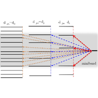
    Cartoon of the energies of the marked states εm within the impurity band. Energy levels are shown with solid black lines forming groups arranged vertically. All states |zm within one group lie at the same Hamming distance djm=d from a given state |zj with d increasing from right to left. The energy level εj is depicted at the right side of the figure with a thick black line. Arrows depict the transitions away from the initial state |ψ(0)=|zj into the marked states |zm whose energy levels lie inside the miniband of the width Γj centered at εj; i.e., they satisfy the condition |εjεm|Γj. The miniband width is indicated with the gray shading area. Arrows of the same color depict transitions within one decay channel, connecting the state |zj to the states a Hamming distance d away from it. Smaller values of d correspond to bigger typical level spacings δεjd [Eq. (87)] and fewer states in a miniband Ωd [Eq. (98)] within the decay channel given by d.

    Reuse & Permissions
  • Figure 15
    Figure 15

    The black solid line shows the plot of the Levy alpha-stable distribution LαC,β(x) [33] with tail index α=1, asymmetry parameter β=1, and unit scale parameter C=1. The inset shows asymptotic behavior of the distribution at large positive x. At x1, the function decays steeply as a double exponential, logL11,1(x)exp[(π/2)x]. The blue line shows the Cauchy distribution L11,0(x)={1/[π(1+x2)]}. We follow here the definition introduced in Ref. [33] and used in subsequent papers on Levi matrices in the physics literature. In the mathematical literature [61, 62], a different definition is usually used, corresponding to f(x;α,β,C1/α,0)=LαC,β(x).

    Reuse & Permissions
  • Figure 16
    Figure 16

    Plot of the PDF gY(x) of the random variable x={(wY2)/[(zε)2+Y2]}, where random variables ε and w obey distributions W1pA(ε/W) and g(w), respectively, and W/(2Y)=30. A detailed discussion of gY(x) is given in Appendix pp12 [see Eq. (l7)]. Its maximum is located at x(Y/W)2. The singularity at x=1 corresponds to ε=z. For large values of x1, the conditional PDF of {Y2/[(zε)2+X2]} is narrowly peaked around its mean value πY/W with |εz|Y, giving rise to the relation in Eq. (109).

    Reuse & Permissions
  • Figure 17
    Figure 17

    The solid line shows the dependence of (w) on α=(1/n)log2w from Eq. (g15). The dashed line shows the tangent to the solid curve at the point α=0 (w=1). This line corresponds to (w)logw, in accordance with Eq. (g24). The inset shows the dependence of the root ρw of Eq. (g12) on α=log2w1/n. Small α1 corresponds to Hamming distances ρw1/2. Near that point, the dependence of ρw on α follows Eq. (g23).

    Reuse & Permissions
  • Figure 18
    Figure 18

    Plot of the PDF of pη(h;0)pη(h) given in Eq. (k6).

    Reuse & Permissions
  • Figure 19
    Figure 19

    Plot of g¯η(z) given in Eq. (l8) for Kη=30.

    Reuse & Permissions
  • Figure 20
    Figure 20

    Probability distribution of the ratio |Y/X| defined in Eqs. (m1) and (m2) for γ=0.6.

    Reuse & Permissions
  • Figure 21
    Figure 21

    The same as in Fig. 20 but with γ=1.2.

    Reuse & Permissions
  • Figure 22
    Figure 22

    The same as in Fig. 20 but for γ=1.6.

    Reuse & Permissions
  • Figure 23
    Figure 23

    K(ω) rescaled with the characteristic energy Γϵ=2ΣtypMϵ where the typical miniband width is given by Eq. (128). Here, γ=1 with fitting exponent ϵ=0.025.

    Reuse & Permissions
  • Figure 24
    Figure 24

    The same as in Fig. 23 but with γ=1.4 and fitting exponent ϵ=0.04.

    Reuse & Permissions
  • Figure 25
    Figure 25

    The same as in Fig. 23 but with γ=1.8 and fitting exponent ϵ=0.05.

    Reuse & Permissions
  • Figure 26
    Figure 26

    The same as in Fig. 23 but with γ=2 and fitting exponent ϵ=0.055.

    Reuse & Permissions
  • Figure 27
    Figure 27

    Population transfer probability as a function of time t in units of 1/Vtyp for various values of parameter γ=2a.

    Reuse & Permissions
  • Figure 28
    Figure 28

    Population transfer probability as a function of time rescaled with the effective miniband width Ω where the number of states in the miniband is estimated using Fermi’s golden rule Ω=M2γ; see Eq. (100) of the main text.

    Reuse & Permissions
×

Sign up to receive regular email alerts from Physical Review X

Reuse & Permissions

It is not necessary to obtain permission to reuse this article or its components as it is available under the terms of the Creative Commons Attribution 4.0 International license. This license permits unrestricted use, distribution, and reproduction in any medium, provided attribution to the author(s) and the published article's title, journal citation, and DOI are maintained. Please note that some figures may have been included with permission from other third parties. It is your responsibility to obtain the proper permission from the rights holder directly for these figures.

×

Log In

Cancel
×

Search


Article Lookup

Paste a citation or DOI

Enter a citation
×