Abstract
We aim at analyzing in terms of a.s. convergence and weak rate the performances of the Multilevel Monte Carlo estimator (MLMC) introduced in [7] and of its weighted version, the Multilevel Richardson–Romberg estimator (ML2R), introduced in [12].
These two estimators permit to compute a very accurate approximation of
1 Introduction
In recent years, there has been an increasing interest in Multilevel Monte Carlo approach which delivers remarkable improvements in computational complexity in comparison with standard Monte Carlo in biased framework. We refer the reader to [8] for a broad outline of the ideas behind the Multilevel Monte Carlo method and various recent generalizations and extensions.
In this paper we establish a Strong Law of Large Numbers and Central Limit Theorem for two kinds of multilevel estimator,
Multilevel Monte Carlo estimator (MLMC) introduced by Giles in [7]
and the Multilevel Richardson–Romberg (weighted) estimator introduced in [12].
We consider a rather general and in some way abstract framework which will allow us to state these results
whatever the strong rate parameter is (usually denoted by β).
To be more precise, we will deal with the versions of these estimators designed to achieve a root mean squared error (RMSE) ε and establish these results as
Let
where
A standard Multilevel Monte Carlo (MLMC) estimator, as introduced by Giles in [7], reads
with
A Multilevel Richardson–Romberg (ML2R) estimator, as introduced in [12], is a weighted version of (1) which reads
with
with the convention
The calibration of the parameters is the result, a root
This calibration has been done in [12] for both estimators MLMC and ML2R under the following assumptions on the sequence
The second one, called strong approximation error assumption, states
Note that the strong error assumption can be sometimes replaced by the sharper
From now on, we set
where the finite real constant
where the finite real constant
The aim of this paper is to prove a Strong Law of Large Numbers (SLLN) and a Central Limit Theorem (CLT) for both estimators MLMC and ML2R calibrated using these optimal parameters. First notice that as these parameters have been computed under the constraint
so that
We will weaken the assumption on the sequence
with
In particular, we will prove that
where
The paper is organized as follows. In Section 2 we briefly recall the technical background for Multilevel Monte Carlo estimators. In Section 3 we stable our main results: a Strong Law of Large Numbers and a Central Limit Theorem in a quite general framework. Section 4 is devoted to the analysis of the asymptotic behavior of the optimal parameters, to the study of the weights of the ML2R estimator and to the bias of the estimators and its robustness. These are auxiliary results that we need for the proof of the main theorems, which we detail in Section 5. In Section 6 we apply these results first to the discretization schemes of Brownian diffusions, where we retrieve recent results by Ben Alaya and Kebaier in [2], and secondly to Nested Monte Carlo.
Notations.
Let
For every
If
We denote by
2 Brief background on MLMC and ML2R estimators
We follow [12] and recall briefly the construction of the optimal parameters derived from the optimization problem (3). The first step is a stratification procedure allowing us to establish the optimal allocation policy
a Multilevel estimator MLMC (1) or ML2R (2) writes
where
Given
using the Schwarz’s inequality (see [12, Theorem 3.6] for a detailed proof). The strong error assumption (${\mathrm{SE}_{\beta}}$) allows us to upper bound
The second step is to select
with
The depth parameter
We report in Tables 1 and 2 the ML2R and MLMC
values for
and
Notice that
Optimal parameters for the ML2R estimator.
Optimal parameters for the MLMC estimator.
In what follows, we will shorter these notations by setting
with
for ML2R and
with
for MLMC.
3 Main results
The asymptotic behavior, as ε goes to 0, of the parameters given in Tables 1 and 2 will be exposed in Section 4. We proceed here to the analysis of the asymptotic behavior of the estimator
3.1 Strong Law of Large Numbers
We will first prove a Strong Law of Large Numbers, namely
Theorem 3.1 (Strong Law of Large Numbers)
Let
Then, for every sequence of positive real numbers
3.2 Central Limit Theorems
A necessary condition for a Central Limit Theorem to hold will be that the ratio between the variance of the estimator and ε converges as
A necessary condition to obtain a CLT is to assume that
3.2.1 Case β > 1
In this case, note that following (${\mathrm{SE}_{\beta}}$) we have
Theorem 3.2 (Central Limit Theorem, β > 1
Assume (${\mathrm{SE}_{\beta}}$) for
with
Then the following statements hold.
ML2R estimator: Assume ((${\mathrm{WE}_{\alpha,\bar{R}}}$)) for all
(12)MLMC estimator: Assume ((${\mathrm{WE}_{\alpha,\bar{R}}}$)) for
Note that the variance of the first term
3.2.2 Case β ∈ ( 0 , 1 ]
In this case, we make the additional sharper assumption that
so that
We conclude that
Theorem 3.3 (Central Limit Theorem, 0 < β ⩽ 1
Assume (${\mathrm{SE}_{\beta}}$) for
Then the following statements hold.
ML2R estimator: Assume ((${\mathrm{WE}_{\alpha,\bar{R}}}$)) for all
(14)MLMC estimator: Assume ((${\mathrm{WE}_{\alpha,\bar{R}}}$)) for
We will see in the proof that the asymptotic variance corresponds to the variance associated to the correcting levels.
3.3 Practitioner’s corner
In the proof of Theorems 3.2 and 3.3 we will obtain the more precise expansion
where
When
When
For ML2R, owing to the expression of
For MLMC, we get
Impact of the weights 𝐖 j R j = 1 , … , R
When
4 Auxiliary results
This section contains some useful results for the proof of the Strong Law of Large Numbers and of the Central Limit Theorem. More in detail, we investigate the asymptotic behavior as
4.1 Asymptotic of the bias parameter and of the depth
An important property of MLMC and ML2R estimators is that
and we recall that this is the optimized bias found in [12] at R fixed.
Since the value of
where
We notice that
The optimal choice for the bias is the projection of
When we replace
Let us analyze the denominator
Since
which yields
For MLMC we may follow the same reasoning starting from
There exists
In what follows, we will always assume that
As
4.2 Asymptotic of the bias and robustness
As part of a Central Limit Theorem, we will be faced to the quantity
is the bias of the estimator.
This leads us to analyze carefully its asymptotic behavior as
The bias of Multilevel estimators is dramatically reduced compared to the Crude Monte Carlo, more precisely the following proposition is proved in [12]:
The following statements hold.
MLMC: Assume ((${\mathrm{WE}_{\alpha,\bar{R}}}$)) with
with
ML2R: Assume ((${\mathrm{WE}_{\alpha,\bar{R}}}$)) for all
where
We notice that the ML2R estimator requires and takes full advantage of a higher order of the expansion of the bias error
(${\mathrm{WE}_{\alpha,\bar{R}}}$),
whereas the MLMC estimator only needs a first order expansion.
As the computations were made under the constraint
and, for MLMC,
We set
For ML2R estimators, if
and
hence
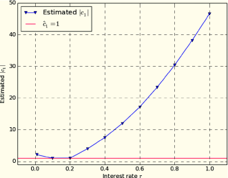
In Figures a and b we show the values of
compared to the value plugged in the simulations
In Figures a and b
we show the absolute value of the empirical bias for different values of r.
In the simulations, we fixed
Estimated
Euler scheme (

Milstein scheme (
Empirical bias
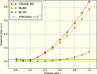
Euler scheme (
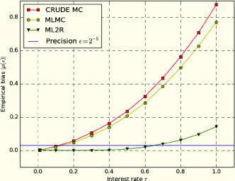
Milstein scheme (
4.3 Properties of the weights of the ML2R estimator
One significant difficulty in the proof of the Central Limit Theorem that we stated in Theorems 3.2 and 3.3,
is to deal with the weights
where the weights
Notice that
where
with the convention
As a consequence,
We will make an extensive use of the following properties, which are proved in Appendix A.
Let
The weights
(19)For every
Let
4.4 Asymptotic of the allocation policy and of the size
Let us analyze the allocation policy
the condition
Owing to Lemma 4.3 (c) with
Moreover, for all
If we set
The asymptotic of the estimator size
We have
Case
Case
where the constant
and
We notice that for
and the factor
Proof.
ML2R: The estimator size N reads
We notice that
MLMC: The result follows directly from the convergence of the series
as desired. ∎
5 Proofs
We will use the notations
where we set
These notations hold for both ML2R and MLMC estimators, where we set
where the bias
5.1 Proof of Strong Law of Large Numbers
The proof of the Strong Law of Large Numbers is a consequence of the following proposition.
Let
Proof.
ML2R: We first give the proof of (23) for the ML2R estimator.
As a first step we show that, for all
By Minkowski’s inequality,
Applying again Minkowski’s inequality, the
As
It follows from the expression of
Then, using that
Owing to Lemma 4.5, up to reducing
Moreover,
Then
with
Hence (23) holds with
MLMC: The proof for the MLMC estimator follows the same steps, by replacing
The Strong Law of Large Numbers follows as a consequence of Proposition 5.1.
Proof of Theorem 3.1.
Owing to the decomposition (22), equation (10) amounts to proving
As
To establish the a.s. convergence of
Hence, by Beppo–Levi’s Theorem,
5.2 Proof of the Central Limit Theorem
This subsection is devoted to the proof of Theorems 3.2 and 3.3.
In order to satisfy a Lindeberg condition, we will need the assumption
Since
One criterion to verify the
The following statements hold.
If there exists a
If there exists a random variable
The family
Now we are in a position to prove the Central Limit Theorem, in both cases
Proof of Theorems 3.2 and 3.3.
Owing to the decomposition (22) (with
where
ML2R: Formulas (12) and (14) amount to proving, as
and
with
In particular, since
which proves (26).
We will use Lindeberg’s Theorem for triangular arrays of martingale increments (see [10, Corollary 3.1, p. 58]) to establish (27). The random variables
Noticing that
The conclusion will follow from
and
Owing to the definition of
Case
and owing to the limit in Lemma 4.3 (d) with
Hence the convergence of the variance (28) holds for Theorem 3.2.
Case
We notice that
if
if
For (29), it follows from the expression of
Owing to the definition of
We conclude by showing that
Owing to the expression of
Moreover, using Lemma 4.5, up to another reduction of
Then (29) is proved and so is the first condition of Lindeberg’s Theorem.
For the second condition of Lindeberg’s Theorem we need to prove that, for every
Since the
We set
where we set
as
and the second condition of Lindeberg’s Theorem is proved.
MLMC:
The proofs are quite the same as for ML2R, up to the constant
We replace
which goes to 0, owing to the strict inequality assumption
6 Applications
6.1 Diffusions
In this subsection we retrieve a recent result by Kebaier and Ben Alaya (see [2]) obtained for MLMC estimators
and we extend it to the ML2R estimators and to the use of path-dependent functionals. Let
where
We know that
with
where
It is classical background that, under the above assumptions on
For the weak error expansion the existing results are less general. Let us recall as an illustration the celebrated Talay–Tubaro’s and Bally–Talay’s weak error expansions for marginal functionals of Brownian diffusions, i.e. functionals of the form
The following statements hold.
Regular setting (Talay–Tubaro [13]): If b and σ are infinitely differentiable with bounded partial derivatives and if
(33)where the coefficients
(Hypo-)Elliptic setting (Bally–Talay [1]): If b and σ are infinitely differentiable with bounded partial derivatives and if σ is uniformly elliptic in the sense that
or more generally if
For more general path-dependent functionals, no such result exists in general. For various classes of specified functionals depending on the running maximum or mean, some exit stopping time, first order weak expansions in
In this subsection we consider
We assume the weak error expansion (${\mathrm{WE}_{\alpha,\bar{R}}}$). We prove now that both estimators ML2R (2) and MLMC (1) satisfy a Strong Law of Large Numbers and a Central Limit Theorem when ε tends to 0.
Let
If
If
As a consequence, both ML2R and MLMC estimators satisfy Theorem 3.3 (case
Proof.
First, note that if F is a Lipschitz continuous functional, with Lipschitz coefficient
then
Assume now that
At this stage it remains to prove (34). The key is [2, Theorem 3], where it is proved that
where
We recall the notations of Jacod and Protter [11]
with
Here
We write, using that
where
Let two bounded Lipschitz continuous functionals be
Since
On the other hand, owing to (32), we prove that
By (36) and Lemma 5.2 (b) we have
with
6.2 Nested Monte Carlo
The aim of a nested Monte Carlo method is to compute by Monte Carlo simulation
where
and we set
where
where
so that
Still assuming that f is Lipschitz continuous. If
As a consequence, assumption (${\mathrm{SE}_{\beta}}$) and the
Proof.
Set
Assume without loss of generality that
Owing to Burkholder’s inequality, there exists a universal constant
Hence, as
Keeping in mind that
We conclude by setting
For the Central Limit Theorem to hold, the key point is the following lemma.
Assume that
Proof.
First note that
Let
with
We derive from the Strong Law of Large Numbers that
and by continuity of the function
We have now to study the convergence of the random sequence
Owing to the Central Limit Theorem and the independence of both terms on the right-hand side of the above inequality, we derive that
where
By Slutsky’s Theorem, we derive from (39), (40) and (41) that for every
Recall that
as desired. ∎
We are now in a position to prove that the nested Monte Carlo satisfies the assumptions of the Central Limit Theorem 3.3.
Assume that
As a consequence, the ML2R and MLMC estimators (2) and (1) satisfy a Central Limit Theorem in the sense of Theorem 3.3 (case
Proof.
We prove first the
Consequently, it suffices to show that
We saw in the proof of Proposition 6.4 that
We notice that
We prove now (43) using again Lemma 5.2 (b) with the convergence in law of
We notice that, if assumption (37) in Proposition 6.3 holds with
6.3 Smooth nested Monte Carlo
When the function f is smooth, namely
It is clear that
Computations similar to those carried out in Proposition 6.3 yield that, if
SLLN:
The first consequence is that the SLLN also holds for these modified estimators along the sequences of RMSE
CLT:
When (44) is satisfied with
which in turn ensures the
As a final remark, note that if the function fis convex,
These results can be extended to locally ρ-Hölder continuous functions with polynomial growth at infinity. For more details and a complete proof we refer to [9].
7 Conclusion
We proved a Strong Law of Large Numbers and a Central Limit Theorem for Multilevel estimators with and without weights and we exhibited two applications: the discretization schemes for diffusions, where we extend a result of Ben Alaya and Kebaier in [2], and the nested Monte Carlo, first mentioned in the Multilevel framework by Lemaire and Pagès in [12]. The Strong Law of Large Numbers is essentially a consequence of the strong error assumption (${\mathrm{SE}_{\beta}}$) (or of its reinforced version (9)), and of the estimator levels’ independence. The understanding of the behavior of the weights in the Multilevel Richardson–Romberg estimator is also crucial at this stage, as it is for the proof of the Central Limit Theorem which follows. Under some additional assumptions of
A Asymptotic of the weights
We focus our attention on the behavior of
with
and with the convention
For convenience, we set
The sequence
Claim (a) of Lemma 4.3 is then proved. As a consequence,
which proves claim (b) in Lemma 4.3. For the proof of claims (c) and (d), we will need the following:
Let
In particular, for all
Proof.
We write
First note that
as
Consequently,
Moreover, by definition we have
as desired. ∎
Proof of Lemma 4.3 (c) and (d).
(c) Let us consider the non-negative measure on
We notice that it is a finite measure since
Since, as we saw in Lemma A.1,
(d) If
If
Owing to Lemma A.1,
If
Let
where
This leads to analyze
Using that
since
References
[1] Bally V. and Talay D., The law of the Euler scheme for stochastic differential equations. I. Convergence rate of the distribution function, Probab. Theory Related Fields 104 (1996), no. 1, 43–60. 10.1007/BF01303802Search in Google Scholar
[2] Ben Alaya M. and Kebaier A., Central limit theorem for the multilevel Monte Carlo Euler method, Ann. Appl. Probab. 25 (2015), no. 1, 211–234. 10.1214/13-AAP993Search in Google Scholar
[3] Billingsley P., Convergence of Probability Measures, 2nd ed., Wiley Ser. Probab. Stat., John Wiley & Sons, New York, 1999. 10.1002/9780470316962Search in Google Scholar
[4] Bujok K., Hambly B. and Reisinger C., Multilevel simulation of functionals of Bernoulli random variables with application to basket credit derivatives, Methodol. Comput. Appl. Probab. 17 (2015), no. 3, 579–604. 10.1007/s11009-013-9380-5Search in Google Scholar
[5] Duffie D. and Glynn P., Efficient Monte Carlo simulation of security prices, Ann. Appl. Probab. 5 (1995), no. 4, 897–905. 10.1214/aoap/1177004598Search in Google Scholar
[6] Gerbi A. A., Jourdain B. and Clément E., Ninomiya–Victoir scheme: Strong convergence, antithetic version and application to multilevel estimators, Monte Carlo Methods Appl. 22 (2016), no. 3, 197–228. 10.1515/mcma-2016-0109Search in Google Scholar
[7] Giles M., Multilevel Monte Carlo path simulation, Oper. Res. 56 (2008), no. 3, 607–617. 10.1287/opre.1070.0496Search in Google Scholar
[8] Giles M. B., Multilevel Monte Carlo methods, Acta Numer. 24 (2015), 259–328. 10.1007/978-3-642-41095-6_4Search in Google Scholar
[9] Giorgi D., Ph.D. thesis, in progress. Search in Google Scholar
[10] Hall P. and Heyde C. C., Martingale Limit Theory and its Application, Probab. Math. Statist., Academic Press, New York, 1980. Search in Google Scholar
[11] Jacod J. and Protter P., Asymptotic error distributions for the euler method for stochastic differential equations, Ann. Probab. 26 (1998), no. 1, 267–307. 10.1214/aop/1022855419Search in Google Scholar
[12] Lemaire V. and Pagès G., Multilevel richardson-romberg extrapolation, preprint 2014, https://arxiv.org/abs/1401.1177v1; to appear in Bernoulli. 10.2139/ssrn.2539114Search in Google Scholar
[13] Talay D. and Tubaro L., Expansion of the global error for numerical schemes solving stochastic differential equations, Stoch. Anal. Appl. 8 (1990), no. 4, 483–509. 10.1080/07362999008809220Search in Google Scholar
© 2017 by De Gruyter