
Sandpile Universality in Social Inequality: Gini and Kolkata Measures


Abstract
:1. Introduction
2. Social Inequality and Its Measures
3. Calculating the Inequality Indices
3.1. Properties of the Lorenz Curve
- The Lorenz curve range from to .Proof.Equation (3) shows see that at , and . Similarly, for , we have and . Hence, as , the Lorenz curve always ranges from to . □
- The Lorenz curve is a concave and monotonically increasing function of wealth.Proof.and,so the slope of the Lorenz curve is given by,As and is always increasing, Equation (6) shows that the slope of the Lorenz curve is always increasing. Hence, the Lorenz curve is a concave and monotonically increasing function of wealth. □
- The Lorenz curve for a society in which each person possesses an equal amount of wealth is a diagonally sloping line.Proof.If each person in a society possesses an equal amount of wealth, wealth distribution follows a Dirac delta function as,Now,Therefore,Again,Hence, we can see that i.e., the Lorenz curve is a diagonal line for this particular case. □
- The upper limit of the Lorenz curve is bounded by the equality line.Proof.According to the second derivative of Equation (6),Therefore, one can conclude from the above exercise that the Lorentz curve can never exceed the diagonal line. Moreover, when and , as . In addition, the concave topology of the Lorentz curve indicates that it is bounded by the diagonal line (also known as the egalitarian line). □
3.2. Exemplary Calculations of the Lorenz Curve
- Uniform wealth distribution: Let us examine a society in which the distribution of income is uniform over a finite range of values within the interval , where . The corresponding probability density function is given by , and the cumulative distribution function is for all values of x within . Applying Equation (3), we obtain the following Lorenz curve for this distribution:The distribution has a mean of , and . It is worth noting that if , the Lorenz curve simplifies to .
- Exponential wealth distribution: Let us consider an exponential income distribution characterized by the probability density function , where , and the cumulative distribution function for all . The mean of this distribution is given by , and . The Lorenz curve for this distribution is therefore given by:
- Pareto wealth distribution: Let us now consider a society with a Pareto-like income distribution. The probability density function for this distribution is given by , and the cumulative distribution function is , where is the minimum income, , and the probability density and cumulative distribution functions are defined for all . The mean of this distribution is , and , which gives the Lorenz curve as follows:
- Discrete wealth distribution: To obtain the Lorenz function for a discrete income distribution, consider an economy comprising G groups of people, where each group (g) comprises individuals with the same income () such that . The total population of the economy is N, and the total income is M, leading to a mean income of . The income distribution is a discrete random variable (X) with a probability mass function of for all g ranging from 1 to G and a distribution function () defined by 0 if , if for any given g ranging from 1 to , and 1 if . We define and as the cumulative proportion of the population and cumulative proportion of the total income, respectively, for each group (g). For any given g ranging from 1 to G and any , it can be verified that . Using the Lorenz function formula, we can calculate the Lorenz function () for any given g ranging from 1 to G and any as,We make two observations in this context. The first observation states that the Lorenz function is piecewise linear, which means that it is composed of several line segments. The kink points represent the points where the direction of the Lorenz curve changes; they occur at the boundaries of each income group. At these points, there is a jump in the cumulative share of income that is distributed to each group, which causes a change in the slope of the Lorenz curve. The second observation is that if there is only one income group in the economy, then the Lorenz curve is a straight line passing through the origin, with a slope of 1. This means that the distribution of income is perfectly equal, and each individual in the economy has the same income. In this case, the Lorenz curve coincides with the diagonal of the unit square, which represents the line .
3.3. Properties of the Gini Index
- Range: The Gini index ranges from 0 to 1, with 0 indicating complete equality (i.e., everyone has the same income or wealth) and 1 indicating complete inequality (i.e., one person has all the income or wealth);
- Normalization: The Gini index is normalized, meaning that it can be used to compare inequality across different populations or over time. This allows for meaningful comparisons even when the populations or time periods have different sizes or levels of income;
- Sensitivity to changes in the distribution: The Gini index is sensitive to changes in the distribution of income or wealth, meaning that even small changes in the distribution can result in large changes in the Gini index. This property makes the Gini index a useful tool for measuring the impact of policies or events that affect the distribution of income or wealth;
- Unimodality: The Gini index is unimodal, meaning that it has a single peak. This property allows for the ranking of populations or time periods based on their level of inequality;
- Invariance to scale: The Gini index is invariant to scale, meaning that it is not affected by changes in the units of measurement (e.g., dollars, euros, etc.). This allows for meaningful comparisons of inequality across populations or time periods using different currencies.
3.4. Exemplary Calculations of the Gini Index
- Uniform wealth distribution: For a uniform distribution on a compact interval , following leads to the following Gini index,
- Exponential wealth distribution: An exponential distribution of the form for any and leads to the following Gini index,
- Pareto wealth distribution: A Pareto distribution of the form with as the minimum income and results in a Gini index of the following form,As we graph the Gini index for various values of , where is greater than 1, we observe that as increases, the Gini index decreases. Additionally, as approaches 1, the Gini index tends towards 1. Furthermore, if we set to be equal to , then the Gini index for is approximately 0.7565.
- Discrete wealth distribution: Consider the discrete random variable discussed previously for which the Lorenz function is given by Equation (12). Accordingly, we have the following explicit form of the Gini index,Note that if for all so that and , then it follows from Equation (16) that,
3.5. Properties of the k-Index
- The k index is a unique fixed point of the complementary Lorenz function.Proof.We can rewrite Equation (5) as,Hence, the k index is a fixed point of the complementary Lorenz function. Since the complementary Lorenz function maps [0, 1] to [0, 1] and is continuous (as shown in Figure 1), it has a fixed point according to Brouwer’s fixed-point theorem. Furthermore, since is non-increasing, the fixed point has to be unique. □
- For any distribution, , and the normalized k index () lies in the interval .Proof.Observe that if , then, according to Equation (18), , and for any other income distribution, . Also note that while the Lorenz curve typically has only two trivial fixed points, that is, and , the complementary Lorenz function () has a unique non-trivial fixed point (k). Now, the normalized k index is given by , so if , then . □
- The k index as a generalization of the Pareto Principle.Proof.The k index can be thought of as a generalization of the Pareto’s 80/20 rule. Note that ; hence, the top of the population has of the income. Hence, the ‘Pareto ratio’ for the k index is . Note that this proportion is derived internally from the distribution of income, and typically, there is no expectation that it will align with the Pareto Principle. □
- Interpreting the k index in terms of rich–poor disparity.Proof.Let us split society into two groups: the ‘poorest’ group, consisting of a fraction (p) of the population, and the ‘rich’ group, consisting of a fraction of the population. Using the Lorenz curve (L(p)), we can determine the distance between the “boundary person” and the poorest person on one hand and the distance between the “boundary person” and the richest person on the other hand. These distances can be calculated using the following equations: and , respectively. The k index is a way of dividing society into two groups such that the boundary person is equidistant from the poorest and richest persons. The disparity function value at the k index is given by . This function measures the gap between the proportion (k) of the poor from the 50/50 population split. If society is not completely equal, then , making it a useful tool to highlight the rich–poor disparity. In this case, k defines the income proportion of the top proportion of the rich population. □
- The k index as a solution to optimization problems.Proof.The k index is the unique solution to the following surplus maximization problem:The value of k is such that it maximizes the area between the complementary Lorenz function and the income distribution line linked with an egalitarian distribution for the lower-income population. Equation (19) is a consequence of the fact that for all and for all . Similarly, the k index is the only solution to the surplus minimization problem (which is the dual of the problem in (19)):Therefore, is the fraction of the higher-income population for which the area between the income distribution line associated with the egalitarian distribution and the Lorenz function is minimized. □
- To reduce inequality between groups, the k index is a better indicator.Proof.The ordering of Lorenz curves based on the k index is not the same as the ordering based on the Gini index. While the Gini index is influenced by transfers only within the poor or rich population, the ranking based on the k index is influenced only by transfers between the two groups. This implies that if the objective is to reduce inequality between the groups, then the k-index is a more appropriate measure to use. □
3.6. Exemplary Calculations of the k Index
- Uniform wealth distribution: Consider a case in which the uniform distribution (F) is defined for , where . Then, the k index is given by,and the normalized k index is given by,
- Exponential wealth distribution: For the exponential distribution (), the complementary Lorenz function is given by . One can show that the k-index is ; hence, the normalized k index is .
- Pareto wealth distribution: For the Pareto distribution (), the complementary Lorenz function is given by . The k index is therefore a solution to the following equation,It is difficult to provide a general solution to this equation. However, we have an interesting observation in this context. If , then the k index is , corresponding to the Pareto principle or the 80/20 rule. Also note that the normalized k index is .
- Discrete wealth distribution: Consider any discrete random variable with the distribution function () discussed above for which the Lorenz function is given by Equation (12). To obtain the explicit form of the k index, one can first apply a simple algorithm to identify the interval of the form defined for in which the k index can lie.Since , if we have in some step, then in the next step, this algorithm has to end, since .Suppose that for any discrete random variable with the distribution function () discussed earlier, Algorithm-1 identifies such that . If , then , and if , is the solution to the following equation:Thus, to derive the k index of any discrete random variable with distribution function , we first my identify the group such that (using Algorithm 1); then, using , we obtain the following value of :
| Algorithm 1: | |
| Step 1: | Consider the smallest such that and consider the sum of . If , then stop, and ; in particular, if and only if . Instead, if , then go to Step 2, consider the group , and repeat the process. |
⋮ | |
| Step t: | Having reached Step t means that in Step , we had . Therefore, consider the sum of . If , then, stop; , and, in particular, if and only if . If , then proceed to Step . |
4. Analytical Studies on the Emerging Coincidence of the Gini and Kolkata Indices
4.1. A Landau-like Phenomenological Expansion of the Lorenz Function
4.2. Some Typical Power Law Forms of Lorenz Functions
4.3. Some Generic Forms of Lorenz Functions
5. Real-World Data Indicating the Convergence of the Gini and Kolkata Indices in Various Socioeconomic Contexts
5.1. Socioeconomic Disparities: An Analysis of Income, Income Tax, and Box Office Earnings Data
5.2. Inequality in Bitcoin Value Fluctuations: A Data Analysis Study
5.3. Inequality Analysis of Vote Data for Election Contestants
5.4. Inequality Analysis for Citation Data of Different Journals and Universities
5.5. A Study of Inequality in Citations: An Analysis of Individual Authors and Award Recipients
5.6. Similarity in the Behavior of the Gini and Kolkata Indices across Multiple Domains: A Universality Study
5.7. Inequality Analysis for Manmade Conflicts and Natural Disasters
5.8. Inequality Analysis in Computing Systems
5.9. Inequality Analysis for Sports: Olympic Medal Share
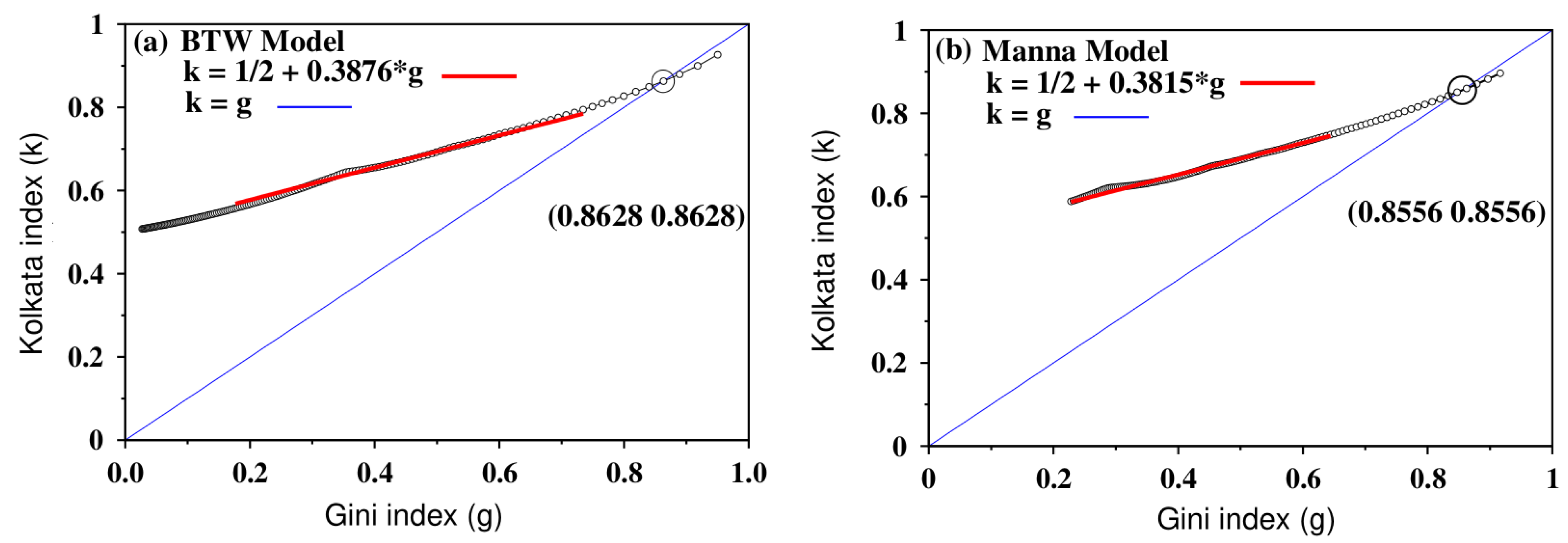
6. Growing Avalanche Size Inequalities in Sand Pile Models: Universality near the SOC Point
7. Summary and Discussion
Author Contributions
Funding
Institutional Review Board Statement
Data Availability Statement
Acknowledgments
Conflicts of Interest
References
- Pareto, V. Cours D’´economie Politique. Reprinted as a Volume of Oeuvres Compl‘etes; Droz: Geneva, Switzerland, 1965; Volume 1896, Available online: https://www.britannica.com/biography/Vilfredo-Pareto (accessed on 1 April 2023).
- Lorenz, M. Methods of measuring the concentration of wealth. Publ. Am. Stat. Assoc. 1905, 9, 209–219. [Google Scholar] [CrossRef]
- Aaberge, R. Characterizations of Lorenz curves and income distributions. Soc. Choice Welf. 2000, 17, 639–653. [Google Scholar] [CrossRef]
- Gini, C.W. Variabilitá e Mutabilitá: Contributo allo Studio delle Distribuzioni e delle Relazioni Statistiche; Cristiano Cuppini: Bologna, Italy, 1912; Available online: https://en.wikipedia.org/wiki/Gini_coefficient#:~:text=The%20Gini%20coefficient%20measures%20the,reflects%20maximal%20inequality%20among%20values (accessed on 1 April 2023).
- Bourguignon, F. Globalization of Inequality; Princeton University Press: Princeton, NJ, USA, 2015. [Google Scholar]
- Available online: https://en.wikipedia.org/wiki/Occupy_Wall_Street (accessed on 1 April 2023).
- Ghosh, A.; Chattopadhyay, N.; Chakrabarti, B.K. Inequality in society, academic institutions and science journals: Gini and k-indices. Physica A 2014, 410, 30–34. [Google Scholar] [CrossRef]
- Banerjee, S.; Chakrabarti, B.K.; Mitra, M.; Mutuswami, S. On the Kolkata index as a measure of income inequality. Physica A 2020, 545, 123178. [Google Scholar] [CrossRef]
- Banerjee, S.; Chakrabarti, B.K.; Mitra, M.; Mutuswami, S. Inequality measures: The kolkata index in comparison with other measures. Front. Phys. 2020, 8, 562182. [Google Scholar] [CrossRef]
- Subramanian, S. Further tricks with the Lorenz curve. Econ. Bull. 2019, 39, 1677–1686. Available online: http://www.accessecon.com/Pubs/EB/2019/Volume39/EB-19-V39-I3-P158.pdf (accessed on 1 April 2023).
- Watkins, N.W.; Pruessner, G.; Chapman, S.C.; Crosby, N.B.; Jensen, H.J. 25 Years of Self-organized Criticality: Concepts and Controversies. Space Sci. Rev. 2016, 198, 3–44. [Google Scholar] [CrossRef]
- Bak, P.; Tang, C.; Wiesenfeld, K. Self-organized criticality: An explanation of 1/f noise. Phys. Rev. Lett. 1987, 59, 381. [Google Scholar] [CrossRef]
- Bak, P. How Nature Works: The Science of Self-Organized Criticality; Copernicus: New York, NY, USA, 1996. [Google Scholar]
- Piketty, T. Capital in Twenty First Century; Harvard University Press: Cambridge, MA, USA, 2017. [Google Scholar]
- Banerjee, S.; Biswas, S.; Chakrabarti, B.K.; Challagundla, S.K.; Ghosh, A.; Guntaka, S.R.; Koganti, H.; Kondapalli, A.R.; Maiti, R.; Mitra, M.; et al. Evolutionary dynamics of social inequality and coincidence of Gini and Kolkata indices under unrestricted competition. Int. J. Mod. Phys. 2023, 34, 2350048. [Google Scholar] [CrossRef]
- Manna, S.S.; Biswas, S.; Chakrabarti, B.K. Near universal values of social inequality indices in self-organized critical models. Phys. A Stat. Mech. Its Appl. 2022, 596, 12721. [Google Scholar] [CrossRef]
- Joseph, B.; Chakrabarti, B.K. Variation of Gini and Kolkata indices with saving propensity in the Kinetic Exchange model of wealth distribution: An analytical study. Phys. A Stat. Mech. Its Appl. 2022, 594, 127051. [Google Scholar] [CrossRef]
- United Nations Development Program. 1992 Human Development Report; Oxford University Press: New York, NY, USA, 1992. [Google Scholar]
- Available online: https://www.irs.gov/statistics/soi-tax-stats-individual-income-tax-returns-publication-1304-complete-report (accessed on 1 April 2023).
- Ludwig, D.; Yakovenko, Y.M. Physics-inspired analysis of the two-class income distribution in the usa in 1983–2018. Phil. Trans. R. Soc. A 2021, 380, 20210162. [Google Scholar] [CrossRef]
- Available online: https://www.boxofficemojo.com/year/2011/ (accessed on 1 April 2023).
- Available online: https://www.bollywoodhungama.com/box-office-collections/filterbycountry/IND/2011/ (accessed on 1 April 2023).
- Available online: https://in.investing.com/crypto/bitcoin/historical-data (accessed on 1 April 2023).
- Available online: https://eci.gov.in/files/file/2785-constituency-wise-detailed-result/ (accessed on 1 April 2023).
- Available online: https://eci.gov.in/files/file/10929-33constituency-wise-detailed-result/ (accessed on 1 April 2023).
- Chatterjee, A.; Ghosh, A.; Chakrabarti, B.K. Universality of Citation Distributions for Academic Institutions and Journals. PLoS ONE 2016, 11, E0146762. [Google Scholar] [CrossRef]
- Chatterjee, A.; Ghosh, A.; Chakrabarti, B.K. Socio-economic inequality: Relationship between Gini and Kolkata indices. Physica A 2017, 466, 583–595. [Google Scholar] [CrossRef]
- Ghosh, A.; Chakrabarti, B.K. Limiting value of the Kolkata index for social inequality and a possible social constant. Phys. A Stat. Mech. Its Appl. 2021, 573, 125944. [Google Scholar] [CrossRef]
- Sinha, A.; Chakrabarti, B.K. Inequality in death from social conflicts: A Gini & Kolkata indices-based study. Phys. A Stat. Mech. Its Appl. 2019, 527, 121185. [Google Scholar] [CrossRef]
- Pressman, R.S. Software Engineering: A Practitioner’s Approach, 7th ed.; McGraw-Hill: Boston, MA, USA, 2010; ISBN 978-0-07-337597-7. [Google Scholar]
- Zimmerman, J. Applying the Pareto Principle (80-20 Rule) to Baseball. 4 June 2010. Available online: https://www.beyondtheboxscore.com/2010/6/4/1501048/applying-the-parento-principle-80 (accessed on 12 April 2018).
- Available online: https://en.wikipedia.org/wiki/2008_Summer_Olympics_medal_table (accessed on 1 April 2023).
- Iglesias, J.R.; Cardoso, B.F.; Gonçalves, S. Inequality, a scourge of the XXI century. Commun. Nonlinear Sci. Numer. Simul. 2021, 95, 105646. [Google Scholar] [CrossRef]
- Boghosian, B.M. Is inequality inevitable? Sci. Am. 2019, 321, 70–77. [Google Scholar]
- Zhukov, D. How the theory of self-organized criticality explains punctuated equilibrium in social systems. Methodol. Innov. 2022, 15, 163. [Google Scholar] [CrossRef]
- Pianegonda, S.; Iglesias, J.R.; Abramson, G.; Vega, J.L. Wealth redistribution with conservative exchanges. Physica A 2003, 322, 667–675. [Google Scholar] [CrossRef]
- Iglesias, J.R.; Gonçalves, S.; Pianegonda, S.; Vega, J.L.; Abramson, G. Wealth redistribution in our small world. Physica A 2003, 327, 12–17. [Google Scholar] [CrossRef]
- Pianegonda, S.; Iglesias, J.R. Inequalities of wealth distribution in a conservative economy. Physica A 2004, 42, 193–199. [Google Scholar] [CrossRef]
- Leydesdorff, L.; Wagner, C.S.; Bornmann, L. Discontinuities in citation relations among journals: Self-organized criticality as a model of scientific revolutions and change. Scientometrics 2018, 116, 623. [Google Scholar] [CrossRef]
- Biondo, A.E.; Pluchino, A.; Rapisarda, A. Order book, financial markets, and self-organized criticality. Chaos Solitons Fractals 2016, 88, 196. [Google Scholar] [CrossRef]
- Biró, T.S.; Telcs, A.; Józsa, M.; Néda, Z. Gintropic scaling of scientometric indexes. Physica A 2023, 618, 128717. [Google Scholar] [CrossRef]
- Minati, G. Big data: From forecasting to mesoscopic understanding. Meta-profiling as complex systems. Systems 2019, 7, 8. [Google Scholar] [CrossRef]
- Brunk, G.G. Self-organized criticality: A new theory of political behaviour and some of its implications. Br. J. Pol. Sci. 2001, 31, 427. [Google Scholar] [CrossRef]
- Ghosh, A.; Biswas, S.; Chakrabarti, B.K. Success of social inequality measures in predicting critical or failure points of some model physical systems. Front. Phys. 2022, 10, 803. [Google Scholar] [CrossRef]
- Korbel, J.; Lindner, S.D.; Pham, T.M.; Hanel, R.; Thurner, S. Homophily-Based Social Group Formation in a Spin Glass Self-Assembly Framework. Phys. Rev. Lett. 2023, 130, 057401. [Google Scholar] [CrossRef]
- Biró, T.S.; Néda, Z. Gintropy: Gini Index Based Generalization of Entropy. Entropy 2020, 22, 879. [Google Scholar] [CrossRef]
- Main, I.G.; Naylor, M. Entropy production and self-organized (sub) criticality in earthquake dynamics. Phil. Trans. R. Soc. A 2010, 368, 131. [Google Scholar] [CrossRef] [PubMed]
- Lang, M.; Shkolnikov, M. Harmonic dynamics of the abelian sandpile. Proc. Natl. Acad. Sci. USA 2019, 116, 2821. [Google Scholar] [CrossRef] [PubMed]


| n | |||
|---|---|---|---|
| p | 0 | ||
| 0.682 | |||
| 0.725 | |||
| 0.667 | 0.755 | ||
| 0.714 | 0.778 | ||
| 0.750 | 0.797 | ||
| 0.778 | 0.812 | ||
| 0.800 | 0.824 | ||
| 0.818 | 0.835 | ||
| 0.833 | 0.844 | ||
| 0.846 | 0.853 | ||
| 0.857 | 0.860 | ||
| 0.867 | 0.866 | ||
| 0.875 | 0.872 | ||
| 0.882 | 0.877 | ||
| 0.889 | 0.882 | ||
| 0.895 | 0.886 | ||
| 0.900 | 0.890 | ||
| 0.905 | 0.894 |
| Case | |||
|---|---|---|---|
| 0.865 | (13, 14) | ||
| 0.869 | (65, 66) | ||
| – | |||
| 0.874 | (17, 18) | ||
| 0.874 | (40, 41) | ||
| 0.877 | (29, 30) | ||
| 0.881 | (77, 78) |
| Movie | Box Office Collection from Hollywood (USA) Movies | ||
|---|---|---|---|
| Release Year | Total Movies | Gini (g) | Kolkata (k) |
| 2010 | 651 | 0.87 | 0.86 |
| 2011 | 730 | 0.87 | 0.87 |
| 2012 | 807 | 0.89 | 0.88 |
| 2013 | 826 | 0.90 | 0.88 |
| 2014 | 849 | 0.90 | 0.88 |
| 2015 | 847 | 0.91 | 0.89 |
| 2016 | 856 | 0.90 | 0.89 |
| 2017 | 852 | 0.91 | 0.89 |
| 2018 | 993 | 0.92 | 0.90 |
| 2019 | 911 | 0.92 | 0.90 |
| Movie | Box Office Collection from Bollywood (India) Movies | ||
| Release Year | Total Movies | Gini (g) | Kolkata (k) |
| 2010 | 139 | 0.77 | 0.81 |
| 2011 | 123 | 0.78 | 0.82 |
| 2012 | 132 | 0.78 | 0.81 |
| 2013 | 136 | 0.76 | 0.79 |
| 2014 | 145 | 0.8 | 0.82 |
| 2015 | 166 | 0.8 | 0.82 |
| 2016 | 215 | 0.83 | 0.83 |
| 2017 | 251 | 0.85 | 0.84 |
| 2018 | 218 | 0.84 | 0.85 |
| 2019 | 246 | 0.85 | 0.86 |
| Year | Total Voters | g | k |
|---|---|---|---|
| 2014 | 0.83 | 0.86 | |
| 2019 | 0.85 | 0.88 |
| Inst./Univ. | Year | ISI Web of Science Data | |||
|---|---|---|---|---|---|
| Index Values | |||||
| Melbourne | 1980 | 866 | 16,107 | 0.67 | 0.75 |
| 1990 | 1131 | 30,349 | 0.68 | 0.75 | |
| 2000 | 2116 | 57,871 | 0.65 | 0.74 | |
| 2010 | 5255 | 63,151 | 0.68 | 0.75 | |
| Tokyo | 1980 | 2871 | 60,682 | 0.69 | 0.76 |
| 1990 | 4196 | 108,127 | 0.68 | 0.76 | |
| 2000 | 7955 | 221,323 | 0.70 | 0.76 | |
| 2010 | 9154 | 91,349 | 0.70 | 0.76 | |
| Harvard | 1980 | 4897 | 225,626 | 0.73 | 0.78 |
| 1990 | 6036 | 387,244 | 0.73 | 0.78 | |
| 2000 | 9566 | 571,666 | 0.71 | 0.77 | |
| 2010 | 15,079 | 263,600 | 0.69 | 0.76 | |
| MIT | 1980 | 2414 | 101,929 | 0.76 | 0.79 |
| 1990 | 2873 | 156,707 | 0.73 | 0.78 | |
| 2000 | 3532 | 206,165 | 0.74 | 0.78 | |
| 2010 | 5470 | 109,995 | 0.69 | 0.76 | |
| Cambridge | 1980 | 1678 | 62,981 | 0.74 | 0.78 |
| 1990 | 2616 | 111,818 | 0.74 | 0.78 | |
| 2000 | 4899 | 196,250 | 0.71 | 0.77 | |
| 2010 | 6443 | 108,864 | 0.70 | 0.76 | |
| Oxford | 1980 | 1241 | 39,392 | 0.70 | 0.77 |
| 1990 | 2147 | 83,937 | 0.73 | 0.78 | |
| 2000 | 4073 | 191,096 | 0.72 | 0.77 | |
| 2010 | 6863 | 114,657 | 0.71 | 0.76 | |
| Inst./Univ. | Year | ISI Web of Science Data | |||
|---|---|---|---|---|---|
| Index Values | |||||
| SINP | 1980 | 32 | 170 | 0.72 | 0.74 |
| 1990 | 91 | 666 | 0.66 | 0.73 | |
| 2000 | 148 | 2225 | 0.77 | 0.79 | |
| 2010 | 238 | 1896 | 0.71 | 0.76 | |
| IISC | 1980 | 450 | 4728 | 0.73 | 0.78 |
| 1990 | 573 | 8410 | 0.70 | 0.76 | |
| 2000 | 874 | 19,167 | 0.67 | 0.75 | |
| 2010 | 1624 | 11,497 | 0.62 | 0.73 | |
| TIFR | 1980 | 167 | 2024 | 0.70 | 0.76 |
| 1990 | 303 | 4961 | 0.73 | 0.77 | |
| 2000 | 439 | 11,275 | 0.74 | 0.77 | |
| 2010 | 573 | 9988 | 0.78 | 0.79 | |
| Calcutta | 1980 | 162 | 749 | 0.74 | 0.78 |
| 1990 | 217 | 1511 | 0.64 | 0.74 | |
| 2000 | 173 | 2073 | 0.68 | 0.74 | |
| 2010 | 432 | 2470 | 0.61 | 0.73 | |
| Delhi | 1980 | 426 | 2614 | 0.67 | 0.75 |
| 1990 | 247 | 2252 | 0.68 | 0.76 | |
| 2000 | 301 | 3791 | 0.68 | 0.76 | |
| 2010 | 914 | 6896 | 0.66 | 0.74 | |
| Madras | 1980 | 193 | 1317 | 0.69 | 0.76 |
| 1990 | 158 | 1044 | 0.68 | 0.76 | |
| 2000 | 188 | 2177 | 0.64 | 0.73 | |
| 2010 | 348 | 2268 | 0.78 | 0.79 | |
| Inst./Univ. | Year | ISI Web of Science Data | |||
|---|---|---|---|---|---|
| Index Values | |||||
| Nature | 1980 | 2904 | 178,927 | 0.80 | 0.81 |
| 1990 | 3676 | 307,545 | 0.86 | 0.85 | |
| 2000 | 3021 | 393,521 | 0.81 | 0.82 | |
| 2010 | 2577 | 100,808 | 0.79 | 0.81 | |
| Science | 1980 | 1722 | 111,737 | 0.77 | 0.80 |
| 1990 | 2449 | 228,121 | 0.84 | 0.84 | |
| 2000 | 2590 | 301,093 | 0.81 | 0.82 | |
| 2010 | 2439 | 85,879 | 0.76 | 0.79 | |
| PNAS(USA) | 1980 | - | - | - | - |
| 1990 | 2133 | 282,930 | 0.54 | 0.70 | |
| 2000 | 2698 | 315,684 | 0.49 | 0.68 | |
| 2010 | 4218 | 116,037 | 0.46 | 0.66 | |
| Cell | 1980 | 394 | 72,676 | 0.54 | 0.70 |
| 1990 | 516 | 169,868 | 0.50 | 0.68 | |
| 2000 | 351 | 110,602 | 0.56 | 0.70 | |
| 2010 | 573 | 32,485 | 0.68 | 0.75 | |
| PRL | 1980 | 1196 | 87,773 | 0.66 | 0.74 |
| 1990 | 1904 | 156,722 | 0.63 | 0.74 | |
| 2000 | 3124 | 225,591 | 0.59 | 0.72 | |
| 2010 | 3350 | 73,917 | 0.51 | 0.68 | |
| PRA | 1980 | 639 | 24,802 | 0.61 | 0.73 |
| 1990 | 1922 | 54,511 | 0.61 | 0.72 | |
| 2000 | 1410 | 38,948 | 0.60 | 0.72 | |
| 2010 | 2934 | 26,314 | 0.53 | 0.69 | |
| PRB | 1980 | 1413 | 62,741 | 0.65 | 0.74 |
| 1990 | 3488 | 153,521 | 0.65 | 0.74 | |
| 2000 | 4814 | 155,172 | 0.59 | 0.72 | |
| 2010 | 6207 | 70,612 | 0.53 | 0.69 | |
| PRC | 1980 | 630 | 19,373 | 0.66 | 0.75 |
| 1990 | 728 | 15,312 | 0.63 | 0.73 | |
| 2000 | 856 | 19,143 | 0.57 | 0.71 | |
| 2010 | 1061 | 11,764 | 0.56 | 0.70 | |
| PRD | 1980 | 800 | 36,263 | 0.76 | 0.80 |
| 1990 | 1049 | 33,257 | 0.68 | 0.76 | |
| 2000 | 2061 | 66,408 | 0.61 | 0.73 | |
| 2010 | 3012 | 40,167 | 0.54 | 0.69 | |
| PRE | 1980 | - | - | - | - |
| 1990 | - | - | - | - | |
| 2000 | 2078 | 51,860 | 0.58 | 0.71 | |
| 2010 | 2381 | 16,605 | 0.50 | 0.68 | |
| Inst./Univ./Journ | Papers (%) | Citations (%) | Comments |
|---|---|---|---|
| Harvard (Univ) | 22 | 78 | About 23% of the papers |
| MIT (Univ) | 22 | 78 | published by leading |
| IISC (Inst) | 25 | 75 | universities/institutions received 77% |
| TIFR (Inst) | 23 | 77 | of the citations. |
| About 19% of the papers | |||
| Nature (Journ) | 18 | 82 | published in leading |
| Science (Journ) | 19 | 81 | journals received 81% of |
| the citations. |
| Award | Name of Recipient | Google Scholar Citation Data | |||
|---|---|---|---|---|---|
| Index Values | |||||
| NOBEL Prize (Econ.) | Joseph E. Stiglitz | 3000 | 323,473 | 0.90 | 0.88 |
| William Nordhaus | 783 | 74,369 | 0.87 | 0.86 | |
| Abhijit Banerjee | 578 | 59,704 | 0.89 | 0.88 | |
| Esther Duflo | 565 | 69,843 | 0.91 | 0.89 | |
| Paul Milgrom | 365 | 102,043 | 0.90 | 0.89 | |
| Paul Romer | 255 | 95,402 | 0.96 | 0.93 | |
| NOBEL Prize (Phys.) | Hiroshi Amano | 1300 | 44,329 | 0.80 | 0.81 |
| David Wineland | 720 | 63,922 | 0.88 | 0.87 | |
| Gérard Mourou | 700 | 49,759 | 0.82 | 0.83 | |
| Serge Haroche | 533 | 40,034 | 0.87 | 0.86 | |
| A. B. McDonald | 492 | 20,346 | 0.91 | 0.88 | |
| David-Thouless | 273 | 47,452 | 0.89 | 0.87 | |
| F.D.M. Haldane | 244 | 41,591 | 0.87 | 0.86 | |
| Donna Strickland | 111 | 10,370 | 0.95 | 0.92 | |
| NOBEL Prize (Chem.) | Joachim Frank | 853 | 48,077 | 0.80 | 0.81 |
| Frances Arnold | 682 | 56,101 | 0.75 | 0.79 | |
| Jean Pierre Sauvage | 713 | 57,439 | 0.73 | 0.77 | |
| Richard henderson | 245 | 27,558 | 0.84 | 0.84 | |
| NOBEL Prize (Bio.) | Gregg L. Semenza | 712 | 156,236 | 0.81 | 0.82 |
| Michael Houghton | 493 | 49,368 | 0.83 | 0.83 | |
| Award | Name of Recipient | Google Scholar Citation Data | |||
|---|---|---|---|---|---|
| Index Values | |||||
| FIELDS Medal (Math.) | Terence Tao | 604 | 80,354 | 0.88 | 0.86 |
| Edward Witten | 402 | 314,377 | 0.74 | 0.79 | |
| Alessio Figalli | 228 | 5338 | 0.67 | 0.75 | |
| Vladimir Voevodsky | 189 | 8554 | 0.83 | 0.85 | |
| Martin Hairer | 181 | 7585 | 0.74 | 0.78 | |
| Andrei Okounkov | 134 | 10,686 | 0.69 | 0.76 | |
| Stanislav Smirnov | 79 | 4144 | 0.76 | 0.79 | |
| Richard E. Borcherds | 61 | 5096 | 0.81 | 0.83 | |
| Ngo Bao Chau | 44 | 1214 | 0.71 | 0.76 | |
| Maryam Mirzakhani | 25 | 1769 | 0.57 | 0.74 | |
| ASICTP DIRAC Medal (Phys.) | Rashid Sunyaev | 1789 | 103,493 | 0.91 | 0.88 |
| Peter Zoller | 838 | 100,956 | 0.81 | 0.82 | |
| Mikhail Shifman | 784 | 52,572 | 0.85 | 0.84 | |
| Subir Sachdev | 725 | 58,692 | 0.83 | 0.82 | |
| Xiao Gang Wen | 432 | 46,294 | 0.8 | 0.82 | |
| Alexei Starobinsky | 328 | 47,359 | 0.81 | 0.82 | |
| Pierre Ramond | 318 | 23,610 | 0.89 | 0.87 | |
| Charles H. Bennett | 236 | 89,798 | 0.9 | 0.88 | |
| V. Mukhanov | 208 | 27,777 | 0.85 | 0.84 | |
| M A Virasoro | 150 | 12,886 | 0.9 | 0.87 | |
| BOLTZMANN Award (Stat. Phys.) | Elliott Lieb | 755 | 76,188 | 0.86 | 0.85 |
| Daan Frenkel | 736 | 66,522 | 0.8 | 0.81 | |
| Harry Swinney | 577 | 46,523 | 0.86 | 0.84 | |
| Herbert Spohn | 446 | 25,188 | 0.79 | 0.8 | |
| Giovanni Gallavotti | 446 | 15,583 | 0.86 | 0.84 | |
| JHON Von NEUMANN Award (Social Sc.) | Daron Acemoglu | 1175 | 172,495 | 0.91 | 0.89 |
| Olivier Blanchard | 1150 | 113,607 | 0.91 | 0.89 | |
| Dani Rodrik | 1118 | 136,897 | 0.9 | 0.89 | |
| Jon Elster | 885 | 79,869 | 0.89 | 0.87 | |
| Jean Tirole | 717 | 201,410 | 0.91 | 0.88 | |
| Timothy Besley | 632 | 57,178 | 0.89 | 0.88 | |
| Maurice Obstfeld | 586 | 73,483 | 0.9 | 0.88 | |
| Alvin E. Roth | 566 | 54,104 | 0.87 | 0.86 | |
| Avinash Dixit | 557 | 82,536 | 0.93 | 0.9 | |
| Philippe Aghion | 490 | 119,430 | 0.85 | 0.85 | |
| Matthew O. Jackson | 397 | 39,070 | 0.86 | 0.84 | |
| Emmanuel Saez | 310 | 48,136 | 0.86 | 0.86 | |
| Mariana Mazzucato | 236 | 12,123 | 0.87 | 0.86 | |
| Glenn Loury | 226 | 13,352 | 0.92 | 0.9 | |
| Susan Athey | 203 | 18,866 | 0.8 | 0.82 | |
| Type of Conflict | g Index | k Index |
|---|---|---|
| War | 0.83 ± 0.02 | 0.85 ± 0.02 |
| Battle | 0.82 ± 0.02 | 0.85 ± 0.02 |
| Armed conflict | 0.85 ± 0.02 | 0.87 ± 0.02 |
| Terrorism | 0.80 ± 0.03 | 0.83 ± 0.02 |
| Murder | 0.66 ± 0.02 | 0.75 ± 0.02 |
| Type of Disaster | g Index | k Index |
|---|---|---|
| Earthquake | ||
| Flood | ||
| Tsunami |
| Year | Medal | g | k |
|---|---|---|---|
| 2020 | Gold | 0.87 | 0.85 |
| Silver | 0.86 | 0.85 | |
| Bronze | 0.84 | 0.84 | |
| Total | 0.84 | 0.83 | |
| 2016 | Gold | 0.88 | 0.87 |
| Silver | 0.86 | 0.85 | |
| Bronze | 0.85 | 0.85 | |
| Total | 0.85 | 0.84 | |
| 2012 | Gold | 0.89 | 0.87 |
| Silver | 0.87 | 0.85 | |
| Bronze | 0.84 | 0.84 | |
| Total | 0.85 | 0.85 | |
| 2008 | Gold | 0.89 | 0.87 |
| Silver | 0.85 | 0.84 | |
| Bronze | 0.86 | 0.85 | |
| Total | 0.85 | 0.84 |
Disclaimer/Publisher’s Note: The statements, opinions and data contained in all publications are solely those of the individual author(s) and contributor(s) and not of MDPI and/or the editor(s). MDPI and/or the editor(s) disclaim responsibility for any injury to people or property resulting from any ideas, methods, instructions or products referred to in the content. |
© 2023 by the authors. Licensee MDPI, Basel, Switzerland. This article is an open access article distributed under the terms and conditions of the Creative Commons Attribution (CC BY) license (https://creativecommons.org/licenses/by/4.0/).
Share and Cite
Banerjee, S.; Biswas, S.; Chakrabarti, B.K.; Ghosh, A.; Mitra, M. Sandpile Universality in Social Inequality: Gini and Kolkata Measures. Entropy 2023, 25, 735. https://doi.org/10.3390/e25050735
Banerjee S, Biswas S, Chakrabarti BK, Ghosh A, Mitra M. Sandpile Universality in Social Inequality: Gini and Kolkata Measures. Entropy. 2023; 25(5):735. https://doi.org/10.3390/e25050735
Chicago/Turabian StyleBanerjee, Suchismita, Soumyajyoti Biswas, Bikas K. Chakrabarti, Asim Ghosh, and Manipushpak Mitra. 2023. "Sandpile Universality in Social Inequality: Gini and Kolkata Measures" Entropy 25, no. 5: 735. https://doi.org/10.3390/e25050735
APA StyleBanerjee, S., Biswas, S., Chakrabarti, B. K., Ghosh, A., & Mitra, M. (2023). Sandpile Universality in Social Inequality: Gini and Kolkata Measures. Entropy, 25(5), 735. https://doi.org/10.3390/e25050735