Research on LSTM-Based Maneuvering Motion Prediction for USVs

Abstract

Maneuvering motion prediction is central to the control and operation of ships, and the application of machine learning algorithms in this field is increasingly prevalent. However, challenges such as extensive training time, complex parameter tuning processes, and heavy reliance on mathematical models pose substantial obstacles to their application. To address these challenges, this paper proposes an LSTM-based modeling algorithm. First, a maneuvering motion model based on a real USV model was constructed, and typical operating conditions were simulated to obtain data. The Ornstein–Uhlenbeck process and the Hidden Markov Model were applied to the simulation data to generate noise and random data loss, respectively, thereby constructing a sample set that reflects real experiment characteristics. The sample data were then pre-processed for training, employing the MaxAbsScaler strategy for data normalization, Kalman filtering and RRF for data smoothing and noise reduction, and Lagrange interpolation for data resampling to enhance the robustness of the training data. Subsequently, based on the USV maneuvering motion model, an LSTM-based black-box motion prediction model was established. An in-depth comparative analysis and discussion of the model’s network structure and parameters were conducted, followed by the training of the ship maneuvering motion model using the optimized LSTM model. Generalization tests were then performed on a generalization set under Zigzag and turning conditions to validate the accuracy and generalization performance of the prediction model.

1. Introduction

Unmanned Surface Vehicles (USVs) have found extensive applications in hydrographic surveying, maritime weather forecasting, coastal port security, and marine environmental monitoring [1]. Reliable maneuverability is fundamental to USV intelligence, as many control algorithms depend on accurate motion prediction, which necessitates a precise understanding of the USV’s motion prediction model. However, the nonlinear and time-varying dynamics of USVs pose significant challenges for model parameter identification and the design of model-based control algorithms [2].

Currently, two primary methods are employed for ship maneuvering modeling. The first is mechanistic modeling, which utilizes either classical Newtonian mechanics or the Lagrange method, combined with fluid dynamics, to establish mathematical models that describe the ship’s dynamic behavior. The main mechanistic models used for ship maneuvering prediction include the Abkowitz model [3], the Maneuvering Modeling Group (MMG) model [4], and the Nomoto model [5]. The Abkowitz model focuses on the influence of hydrodynamic forces and moments in the ship’s maneuvering equations, while the MMG model decomposes the hydrodynamic forces into components acting on the hull, propeller, and rudder, considering their interactions. The Nomoto model, which describes the ship’s posture and motion response using a set of differential equations, is valued for its simplicity and ease of understanding, although it has limitations in precision [6]. Zou Zaojian applied Support Vector Machines (SVMs) to identify hydrodynamic derivatives and moments within the Abkowitz model, enhancing the accuracy of ship maneuvering predictions [7]. However, Xu developed an optimal truncated LS-SVM method [5,8], validated through self-propelled experiments [9], though their study did not address scale effects. Pandey described a three-degree-of-freedom (3DoF) MMG mathematical model for the Wave Adaptive Modular Vessel (WAM-V) [10], using a combination of captive model testing and system identification to calculate maneuvering derivatives, with the MMG model simulations demonstrating good performance in turning characteristics. Nonetheless, issues like ocean disturbances remain unresolved. Luo W. et al. [11] utilized a two-layer feedforward neural network to identify the maneuverability indices and linear hydrodynamic derivatives within the linear MMG model, demonstrating the stability of the estimated parameters. However, the study involved significant simplifications of the MMG model, and the accuracy of parameter identification remains to be improved. Carrillo S. et al. [12] conducted ship motion modeling based on the Nomoto maneuvering model and used the least squares method to identify the KT parameters.

The second modeling approach is black-box modeling. This method measures the input and output data of a maneuvering ship, and establishes a model that describes the input-output characteristics during ship maneuvering through appropriate processing and computation. Notably, this approach does not require detailed descriptions of the dynamic characteristics of the maneuvering process. In the identification work using white-box models, the task primarily involves identifying coefficients or parameters within a predetermined model, thus making the accuracy of identification dependent on the limitations of the mathematical model [13]. Using fixed, linear, and time-invariant mathematical models for ship maneuvering makes it challenging to generalize predictions, as these models fail to capture the complex nonlinear characteristics of ship motions. When the mathematical model is highly complex, the number of parameters to be identified becomes excessive, relying heavily on a large volume of high-quality sample data. It becomes difficult to obtain accurate model parameters in the presence of disturbances or irregular sample data [14]. Additionally, the precision of hydrodynamic parameter calculations for the hull, propeller, and rudder significantly affects the accuracy of motion predictions. Moreover, factors such as design and manufacturing errors, equipment wear during operation, the maneuvering environment, and variations in ship loading can all contribute to inaccuracies in the ship’s motion model throughout a ship’s lifecycle. These inaccuracies limit the effectiveness of using white-box models for motion prediction. However, employing white-box models can aid in improving the original mathematical models. Bonci et al. [15] improved the fully nonlinear Abkowitz model by identifying the USV model through CFD free-running simulations. This work utilized high-precision CFD data to eliminate the typical characteristic noise present in outdoor tank experiment data.

Over the past decade, numerous machine learning methods have demonstrated remarkable performance in the field of system identification [16], including Support Vector Regression (SVR) [17], Least Squares Support Vector Machines (LSSVM) [18], and Wavelet Neural Networks (WNN) [16]. Zou Zaojian [19] proposed a black-box modeling method based on BP neural networks for the 3-DOF ship maneuvering model, validating the potential of network-based models as control models or state observers in the domain of ship motion control. This method utilized a fully connected neural network to establish a black-box model of 3-DOF ship maneuvering, requiring only three maneuvering operations to identify and validate the model. However, the study did not account for environmental disturbances in the black-box model. Additionally, a black-box offline modeling method for ship maneuvering was proposed using Multi-Output $\nu$ Support Vector Regression (MO-$\nu$-SVR), which optimized the computational efficiency and operability of traditional SVR models. Nevertheless, the research did not consider external disturbances that might influence the dynamic characteristics of the ship. Liu et al. [20], based on free-sailing experiments with the KVLCC2 ship model and a multi-degree-of-freedom Wave Energy Converter (WEC), proposed three identification frameworks: parametric grey-box modeling, non-parametric grey-box modeling, and Bayesian regression-based black-box modeling. They summarized the prerequisites for using these frameworks and demonstrated that the black-box model constructed through Bayesian regression exhibited stronger generalization ability in the loss function compared to SVM and ANN, due to the incorporation of prior knowledge. However, the wave energy training set used in the study was based on regular waves, which limits its generalizability.

In conclusion, the development of ship maneuverability prediction is characterized by diverse modeling approaches, data-driven methodologies, and an emphasis on model accuracy and generalization capabilities. Simultaneously, experimental methods and data validation techniques are continually being refined. As technology advances, research into ship maneuverability will become more in-depth and sophisticated, providing more reliable theoretical support for ship design and operation. Intelligent algorithms also hold significant promise in this field; however, challenges such as extensive training time, complex parameter tuning processes, and heavy reliance on mathematical models pose substantial obstacles to their application. To address these challenges, this paper proposes a Long Short-Term Memory Network (LSTM)-based modeling algorithm for USV maneuvering. By learning from historical USV motion data, the model developed in this study captures the maneuvering characteristics of the USV through machine learning. The subsequent sections of this paper are organized as follows: In Section 2, a maneuvering motion model based on a real USV model was constructed to obtain sample data. The sample data were then pre-processed for training. In Section 3, an LSTM-based black-box motion prediction model was established. In Section 4, an in-depth comparative analysis and discussion of the model’s network structure and parameters were conducted, followed by the training of the ship maneuvering motion model using the optimized LSTM model.

2. Sample Data Set Construction and Data Processing

2.1. The Maneuvering Motion Model of USV

The 3-DOF MMG motion model of the USV is described as follows:

$$\left\{\begin{array}{c}\dot{x}=ucos\phi -vsin\phi \\ \dot{y}=usin\phi +vcos\phi \\ \dot{\phi }=r\\ \dot{u}={\displaystyle \frac{1}{m+m_x}}\left[\left(m+m_y\right)rv+X_H+X_P+X_R\right]\\ \dot{v}={\displaystyle \frac{1}{m+m_y}}\left[-\left(m+m_x\right)rv+Y_H+Y_P+Y_R\right]\\ \dot{r}={\displaystyle \frac{1}{I_{zz}+J_{zz}}}\left(N_H+N_P+N_R\right)\end{array}\right.$$

(1)

where x and y are the coordinates of the USV in the geodetic coordinate system, $u$ is the longitudinal velocity, $v$ is the lateral velocity, $r$ represents the rate of angular, φ is the angle of the heading, $m_x$ is the additional longitudinal mass, $m_y$ is the additional transverse mass, and $I_{zz}$ is the inertia moment of yaw. $J_{zz}$ is the additional moment of inertia in yaw. X, Y, and N represent hydrodynamic forces and moments, while the subscripts H, P, and R represent the hull, propeller, and rudder, respectively.

The approximate model for calculating $X_{calm}$, $Y_{calm}$, $N_{calm}$ was established using the MMG model:

$$\left\{\begin{array}{c}{X}_{calm}=X_H+X_P+X_R\\ Y_{calm}=Y_H+Y_R\\ N_{calm}=N_H+N_R\end{array}\right.$$

(2)

The force acting on the hull is approximate to the hydrodynamic derivative $X_H$, $Y_H$, $N_H$, and can be expressed as

$$\left\{\begin{array}{c}{X}_H=X_0+X_u\Delta u+X_{uu}{\left(\mathsf{\Delta }u\right)}^2+X_{uuu}{\left(\mathsf{\Delta }u\right)}^3+X_{vv}{v}^2+X_{rr}{r}^2+X_{vr}vr\\ Y_H=Y_{v}v+Y_{vvv}{v}^3+Y_{\dot{v}}\dot{v}+Y_{r}r+Y_{rrr}{r}^3+Y_{\dot{r}}\dot{r}+Y_{vrr}v{r}^2+Y_{vvr}{v}^{2}r\\ N_H=N_{v}v+N_{vvv}{v}^3+N_{\dot{v}}\dot{v}+N_{r}r+N_{rrr}{r}^3+N_{\dot{r}}\dot{r}+N_{vrr}v{r}^2+N_{vvr}{v}^{2}r\end{array}\right.$$

(3)

where $\mathsf{\Delta }u=u-u_0$ is the speed difference of the ship relative to the initial ship speed, and ${-X}_0$ is the resistance when the speed of ship is $u_0$. The model of the USV used in this study is depicted in Figure 1. The parameters of the USV can be found in reference [18].

2.2. Sample Data Acquisition

According to Equation (1), simulations of zigzag and turning maneuvers were conducted for the USV under both still water and wave conditions, with a time step of 0.1 s. These simulations covered rudder angles ranging from 10° to 35°, ensuring the availability of the motion data necessary for subsequent maneuverability predictions. In the simulations, the wave conditions were characterized by a wavelength of 5 m and a wave height of 0.3 m. The conditions of simulation are listed in

Table 1. Conditions of simulations.

Scenarios	Conditions
No Wave	10°/10° Zigzag
	15°/15° Zigzag
	20°/20° Zigzag
	25° Turning
	30° Turning
	35° Turning
Wave	10°/10° Zigzag
	15°/15° Zigzag
	20°/20° Zigzag
	25° Turning
	30° Turning
	35° Turning

.

Due to the inherent noise present in ship trials, noise errors primarily arise from sensor inaccuracies related to angles, positioning, and other measurements. The UWB positioning system may also experience data loss and inaccuracies due to interference from scatterers, water surface, and ferromagnetic materials. Additionally, wireless signals may encounter indeterminate additional delays when penetrating obstacles. Consequently, noise was added to the simulation data, and a portion of the data points were randomly discarded to simulate the errors, high-frequency disturbances, and data acquisition losses typically encountered in ship trials.

By combining the Ornstein–Uhlenbeck (OU) process for noise and the Hidden Markov Model (HMM) for data loss, the ith final simulated data ${\mathit{x}}_i^{\left(simu\right)}$ is expressed as

$${\mathit{x}}_i^{\left(simu\right)}, {\mathit{y}}_i^{\left(simu\right)}=\left\{\begin{array}{cc}{\mathit{x}}_i^{\left(noisy\right)}, {\mathit{y}}_i^{\left(noisy\right)}& if the HMM is in state S_1\\ NULL& if the HMM is in state S_2\end{array}\right.$$

(4)

where ${\mathit{x}}_i^{\left(simu\right)},{\mathit{y}}_i^{\left(simu\right)}$ is the data added with OU noise. Take $\mathit{x}$ as an example:

$${\mathit{x}}_i^{\left(noisy\right)}={\mathit{x}}_i^{\left(ideal\right)}+{\mathit{x}}_i^{\left(OU\right)}$$

(5)

where ${\mathit{x}}_i^{\left(ideal\right)}$ is the data from the conditions form simulation shown in Table 1, and ${\mathit{x}}_i^{\left(OU\right)}$ represents OU noise. OU noise is a time-correlated stochastic process initially used to describe Brownian motion in physics. In RL, it is employed to generate smooth and orderly noise sequences that aid in exploring the action space. The mathematical expression for the OU process is

$${d\mathit{x}}_i=\theta (\mu -{\mathit{x}}_i)dt+\sigma d{\mathit{W}}_i$$

(6)

where ${\mathit{x}}_i^{\left(OU\right)}$ is the ith value of the noise at time $t$. $\theta$ is the parameter controlling the speed of noise regression to the mean. $\mu$ is the long-term mean of the noise. $\sigma$ is the intensity of noise fluctuations. $d{\mathit{W}}_i$ is the standard Brownian motion.

At each time step, the noise is updated according to the following OU process:

$${\mathit{x}}_{i+1}={\mathit{x}}_i+\theta (\mu -{\mathit{x}}_i)\mathsf{\Delta }t+\sigma \sqrt{\mathsf{\Delta }t}\mathcal{N}(\mathrm{0,1})$$

(7)

where $\mathcal{N}\left(\mathrm{0,1}\right)$ is a normal distribution with mean 0 and variance 1. When executing the strategy, the generated OU noise is added to the actions derived from the deterministic strategy.

$S_1$ and $S_2$ in Formula (4) are two states in the HMM, which is employed to represent the states of data transmission, where the states represent whether the data is successfully received or lost. HMM is used for modeling systems that have unobservable states with observable outcomes. $S_1$ indicates that the data is successfully transmitted, and $S_2$ indicates that the data is lost. The transition probabilities between these states are given by the matrix $P$:

$$P=\left(\begin{array}{cc}{P}_{11}& P_{12}\\ P_{21}& P_{22}\end{array}\right)$$

(8)

where $P_{ij}$ represents the probability of transitioning from state $S_i$ to state $S_j$.

2.3. Sample Data Processing

In the USV motion data samples obtained, the different elements of the input vector should hold equal importance; however, differing scales among these elements can influence how regression algorithms assess their significance. Therefore, before model training, the input vectors were normalized using the following:

$$\begin{array}{c}{\mathit{X}}^{\left(formal\right)}={\mathit{X}}^{\left(simu\right)}./\max (|{\mathit{X}}^{\left(simu\right)}|)\\ {\mathit{Y}}^{\left(formal\right)}={\mathit{Y}}^{\left(simu\right)}./\max (|{\mathit{Y}}^{\left(simu\right)}|)\end{array}$$

(9)

where ${\mathit{X}}^{\left(formal\right)}$ denotes the normalized input matrix, and ${\mathit{Y}}^{\left(formal\right)}$ denotes the normalized output matrix. ${\mathit{X}}^{\left(formal\right)}$={$x_i^{\left(formal\right)}|i=\mathrm{1,2},...N$}. For simplification of the equations, $x$ will be used to represent $x^{\left(formal\right)}$ in subsequent discussions, and the same applies to the simplification of $y^{\left(formal\right)}$.

Disregarding factors such as speed fluctuations during ship trials allows the ship model’s motion to be approximated as a discrete linear dynamic system. A Kalman filter was employed for preliminary filtering of the system:

$${\mathit{x}}_i=\mathit{A}\times {\mathit{x}}_{i-1}+\mathit{B}\times {\mathit{u}}_i+{\mathit{\omega }}_{i-1}$$

(10)

$${\mathit{z}}_i=\mathit{H}\times {\mathit{x}}_i+{\mathit{v}}_i$$

(11)

where $x_i$ represents the system state matrix, $z_i$ is the observed state matrix, $A$ is the state transition matrix, $B$ is the control input matrix, $H$ is the observation matrix, $\omega$ is the process noise, and $v$ is the measurement noise. Both $\omega$ and $v$ are assumed to follow Gaussian white noise distributions with covariances $Q$ and $R$, respectively. The parameters are $\mathit{Q}={\mathsf{\sigma }}_{\mathrm{Q}}^2\times [\begin{array}{cc}\mathrm{q}& 0\\ 0& \mathrm{q}\end{array}]$, $\mathit{q}=[\begin{array}{cc}{\displaystyle \frac{1}{4}}{\Delta \mathrm{t}}^4& {\displaystyle \frac{1}{2}}{\Delta \mathrm{t}}^3\\ {\displaystyle \frac{1}{2}}{\Delta \mathrm{t}}^3& {\Delta \mathrm{t}}^2\end{array}]$; $\mathit{R}=\left[\begin{array}{cc}{\mathsf{\sigma }}_{\mathrm{R}}^2& 0\\ 0& {\mathsf{\sigma }}_{\mathrm{R}}^2\end{array}\right]$ where ${\mathsf{\sigma }}_{\mathrm{Q}}=1$, ${\mathsf{\sigma }}_{\mathrm{R}}=20$, with $\Delta \mathrm{t}$ representing the data sampling interval.

Subsequently, Lagrange polynomial interpolation was applied to reconstruct missing data points in the case of lost ship motion data samples in discrete signals. For each known data point, a corresponding Lagrange basis polynomial was constructed:

$$l_i(t)=\prod _{\begin{array}{c}j=1\\ j\ne i\end{array}}^n{\displaystyle \frac{t-t_j}{t_i-t_j}}$$

(12)

The Lagrange interpolation polynomial was then obtained by summing the weighted basis functions:

$$L(t)=\sum _{i=1}^{n}x(t_i)l_i(t)$$

(13)

Finally, substituting $t=t_m$ into the interpolation polynomial $L\left(t\right)$ provides the estimated value of $x\left(t_m\right)$:

$$x(t_m)=\sum _{i=1}^{n}x(t_i)l_i(t_m)$$

(14)

where $l_i\left(t_m\right)$ is the value of the i-th basis polynomial where $t=t_m$.

To ensure the robustness of the sample data, a radial reach filter (RRF) was applied for further processing of the filtered data. The first step involves forward filtering to obtain the initial filtered signal, which is then reversed in the time domain. The reversed signal undergoes a second filtering process, and, finally, the output is reversed again in the time domain to obtain a radial reach filtered signal. This signal has zero phase distortion, and its amplitude-frequency characteristics are corrected by the square of the filter’s amplitude-frequency response.

Let $z$ represent the frequency domain, where $z=e^{jw}$. The process can be expressed by the following equations:

$$\left.\begin{array}{c}{Y}_1\left(e^{jw}\right)=X\left(e^{jw}\right)H\left(e^{jw}\right) \\ Y_2\left(e^{jw}\right)=e^{-jw\left(N-1\right)}{Y}_1\left(e^{-jw}\right) \\ Y_3\left(e^{jw}\right)=Y_2\left(e^{jw}\right)H\left(e^{jw}\right) \\ Y\left(e^{jw}\right)=e^{-jw\left(N-1\right)}{Y}_3\left(e^{-jw}\right) \end{array}\right\}$$

(15)

where $X\left(e^{jw}\right)$ is the input, $Y\left(e^{jw}\right)$ is the output, $H\left(e^{jw}\right)$ is the impulse response sequence, and $Y_i\left(i=\mathrm{1,2},3\right)$ represents the intermediate response. The RRF effectively eliminates phase distortion, providing an accurate representation of data trends. However, it requires the “time-reversal” of the signal sequence, which implies that it cannot be used for real-time data processing. Therefore, this method is only suitable for offline data processing, where the complete experimental data is collected first, followed by filtering and comparison with simulation tests.

The dataset was split into a 9:1 ratio for the training set and test set, with the test set used for the final evaluation of the model’s overall generalization performance to ensure robust performance on unseen data. To prevent overfitting, a portion of the training data was extracted to form a validation set, which was used for preliminary evaluation and hyperparameter tuning of the model. During training, the validation set performance was monitored to determine whether training should be halted. This study employed the K-fold cross-validation method.

3. LSTM-Based USV Motion Black-Box Prediction Model

The velocities $u$, $v$ and angular velocity $r$ in Equation (1) were discretized using the Euler difference method, leading to the iterative equations that predict the motion from time step k to k + 1, as represented by Equations (16) through (18):

$$\begin{array}{cc}\hfill u\left(k+1\right)=u\left(k\right)& +{\displaystyle \frac{h}{m+m_x}}[X_{u}u\left(k\right)-2u_0{X}_{uu}u\left(k\right)+3X_{uuu}{u}_0^{2}u\left(k\right)\hfill \\ & +{X_{uu}u}^2\left(k\right)-3X_{uuu}{u}^2\left(k\right)u_0+{X_{uuu}u}^3\left(k\right)+X_{vv}{v}^2\left(k\right)\\ & +X_{rr}{r}^2\left(k\right)+X_{vr}v\left(k\right)r\left(k\right)+\left(m+m_y\right)v\left(k\right)r\left(k\right)-{X_{uuu}u}_0^3\\ & +{X_{uu}u}_0^2-X_u{u}_0+X_0+X_P+X_R]\end{array}$$

(16)

$$\begin{array}{cc}\hfill v\left(k+1\right)=v\left(k\right)& +{\displaystyle \frac{h}{m+m_y-Y_{\dot{v}}}}[Y_{v}v\left(k\right)+Y_{vvv}{v}^3\left(k\right)+Y_{r}r\left(k\right)\hfill \\ & -{\displaystyle \frac{Y_{\dot{r}}}{m+m_y-Y_{\dot{v}}}}r\left(k\right)+Y_{rrr}{r}^3\left(k\right)-\left(m+m_x\right)v\left(k\right)r\left(k\right)\\ & +Y_{vrr}v{\left(k\right)r}^2\left(k\right)+Y_{vvr}{v}^2\left(k\right)r\left(k\right)+Y_R]\\ & +{\displaystyle \frac{Y_{\dot{r}}}{m+m_y-Y_{\dot{v}}}}r\left(k+1\right)\end{array}$$

(17)

$$\begin{array}{cc}\hfill r\left(k+1\right)=r\left(k\right)& +{\displaystyle \frac{h}{I_{zz}+J_{zz}-N_{\dot{r}}}}(N_{v}v\left(k\right)-{\displaystyle \frac{N_{\dot{v}}}{I_{zz}+J_{zz}-N_{\dot{r}}}}v\left(k\right)+N_{vvv}{v}^3\left(k\right)\hfill \\ & +N_{r}r\left(k\right)+N_{rrr}{r}^3\left(k\right)+N_{vrr}v\left(k\right)r^2\left(k\right)+N_{vvr}{v}^2\left(k\right)r\left(k\right)\\ & +N_R)+{\displaystyle \frac{N_{\dot{v}}}{I_{zz}+J_{zz}-N_{\dot{r}}}}v\left(k+1\right)\end{array}$$

(18)

From these equations, the following black-box prediction model was developed:

$$\left\{\begin{array}{c}u\left(k+1\right)={\rho }_1\left(u\left(k\right),v\left(k\right),r\left(k\right),\delta \left(k\right)\right)\\ v\left(k+1\right)={\rho }_2\left(u\left(k\right),v\left(k\right),r\left(k\right),\delta \left(k\right)\right)\\ r\left(k+1\right)={\rho }_3\left(u\left(k\right),v\left(k\right),r\left(k\right),\delta \left(k\right)\right)\end{array}\right.$$

(19)

where $\mathsf{\rho }(\cdot )$ represents a nonlinear vector function describing the nonlinear relationship between the input and output of samples. $\mathit{x}$ denotes the input matrix composed of input vectors ${\mathit{x}}_{\mathit{i}}$, $\mathit{x}={\left[{\mathit{x}}_1,\cdots {\mathit{x}}_{\mathit{i}},\cdots ,{\mathit{x}}_{\mathit{N}}\right]}^T$; ${\mathit{x}}_{\mathit{i}}=\left[u_i,v_i,r_i,{\delta }_i\right]$, with the superscript $T$ indicating matrix transposition; $\mathit{y}$ represents the output matrix composed of output vectors ${\mathit{y}}_i$, ${\mathit{y}}_{\mathit{i}}=\left[{\mathit{u}}_{\mathit{i}},{\mathit{v}}_{\mathit{i}},{\mathit{r}}_{\mathit{i}}\right]$. The index $i$ corresponds to the $i$-th data point, with $i$ ranging from 1 to $N$, where $N$ is the number of sample points in the sample set $S$, and $t_i$ is the corresponding time.

This black-box model reveals the nonlinear mapping relationship between the ship’s motion variables and the rudder angle. The system’s inputs are represented by the vector $\{u\left(k\right),v\left(k\right),r\left(k\right),\delta \left(k\right)\}$, corresponding to the outputs $\{u\left(k+1\right),v\left(k+1\right),r\left(k+1\right)\}$. Therefore, the input and output vectors for the black-box modeling can be expressed as

$$\left\{\begin{array}{cc}\hfill input:& [u\left(k\right),v\left(k\right),r\left(k\right),\delta \left(k\right)]\hfill \\ \hfill output:& [u\left(k+1\right),v\left(k+1\right),r\left(k+1\right)]\hfill \end{array}\right.$$

(20)

A schematic of the machine learning-based black-box modeling and motion prediction process is presented in Figure 2. At each step, the input vector $[u\left(k\right),v\left(k\right),r\left(k\right),\delta \left(k\right)]$ is fed into the LSTM, and the corresponding output in LSTM represents the USV motion output vector $y_t$.

LSTM is a variant of Recurrent Neural Networks (RNNs), specifically designed to address the issues of vanishing and exploding gradients encountered in traditional RNNs when dealing with long sequences. The primary characteristic of LSTM is its ability to capture and retain long-term dependencies, enabling effective learning and memory of information when processing long sequence data. The LSTM architecture comprises input gates, forget gates, output gates, and memory cells, which control the flow of information and allow the LSTM model to selectively retain or discard previous information. This design enables LSTM to capture long-term dependencies more effectively when processing long sequences, thereby improving model performance. Each LSTM unit in the continuous sequence shares the same parameters, with inputs and outputs corresponding to adjacent time steps in the time series. At time step $t$, the network’s input is $X_t$, the memory cell is $C_t$, and the output is the hidden state $h_t$.

The core of LSTM lies in the forget gate, which determines which parts of the previous memory should be retained and which should be discarded, enabling autonomous learning without external intervention. The forget gate takes the current input $X_t$ and the previous hidden state $h_{t-1}$ as inputs, and outputs a decay coefficient $f_t$ (ranging from 0 to 1) that represents the proportion of information retained. The calculation of the forget gate is given by Equation (21):

$$f_t=\mathrm{s}\mathrm{i}\mathrm{g}\mathrm{m}\mathrm{o}\mathrm{i}\mathrm{d}(W_f\cdot [h_{t-1},X_t]+b_f)$$

(21)

where $h_{t-1}$ is the hidden state of the previous LSTM unit, $X_t$ is the current input, and $W_f$ and $b_f$ are used for the linear transformation before the sigmoid function is applied. The input gate determines how much new information should be added to the memory cell $C_t$. The input gate takes the current input $X_t$ and the previous hidden state $h_{t-1}$ as inputs, and outputs the memory decay coefficient $i_t$ and the learned memory content $\widetilde{C_t}$. The memory decay coefficient $i_t$ calculated by the sigmoid layer and the memory content $\widetilde{C_t}$, generated by the tanh layer, are given by Equations (22) and (23), respectively:

$$i_t=\mathrm{s}\mathrm{i}\mathrm{g}\mathrm{m}\mathrm{o}\mathrm{i}\mathrm{d}(W_i\cdot [h_{t-1},X_t]+b_i)$$

(22)

$$\widetilde{C_t}=\tanh (W_c\cdot [h_{t-1},X_t]+b_c)$$

(23)

The memory cell $C_t$ of LSTM is updated using the outputs of the forget gate and the input gate, as shown in Equation (24):

$$C_t=f_t\times C_{t-1}+i_t\times \widetilde{C_t}$$

(24)

Finally, the hidden state $h_t$ of the LSTM unit is determined based on the memory cell $C_t$. First, the sigmoid layer determines which memory cells $C_t$ will be activated for output, represented by $o_t$. Then, the memory cell $C_t$ is processed by the tanh function to obtain a value between −1 and 1, which is multiplied by the output of the sigmoid gate to obtain the final output $h_t$. The calculations for $o_t$ and the final output $h_t$ are shown in Equations (25) and (26):

$$o_t=\mathrm{s}\mathrm{i}\mathrm{g}\mathrm{m}\mathrm{o}\mathrm{i}\mathrm{d}(W_0\cdot [h_{t-1},X_t]+b_0)$$

(25)

$$h_t=o_t\times \tanh \left(C_t\right)$$

(26)

The outputs $C_t$ and $h_t$ at time t are used as inputs for the next time step. In a multi-layer stacked LSTM model, the output sequence from the previous layer is used as input for the next layer. The output of the last layer, specifically the hidden state $h_t$ at the final time step, represents the predicted USV motion state.

During the model training process, the difference between the predicted values and the actual values is analyzed to facilitate self-learning based on predefined rules. The model optimizes itself by adjusting internal parameters to achieve the best performance. The model is updated with the goal of minimizing the prediction error. Since this model update involves a non-convex optimization problem, it is challenging to reliably search for the global optimal solution using gradient descent. To enhance the global search capability of gradient descent, the Adam optimization algorithm is employed. Adam combines the concepts of momentum and RMSprop, taking into account both first-order and second-order moment estimates of the gradients, thereby improving the effectiveness of gradient descent in non-convex optimization problems. The root mean square error (RMSE) and correlation coefficient (CC) are used to comprehensively evaluate the prediction accuracy of the model. RMSE is used to compare the differences between predicted and actual observed values, with smaller differences indicating better predictive performance. CC measures the strength and direction of the linear relationship between the predicted and actual observed values. When the CC between the model’s predicted data and the actual data approaches 1, it indicates a high degree of consistency between the predicted and actual data, resulting in improved predictive performance.

To validate the generalization of the LSTM-based black-box model, the trained model is used to predict the generalization set, and the predicted values are compared with the expected values. Since the trained model already possesses motion prediction capabilities, only the initial ship state $\left[\mathrm{u}\right(0),\mathrm{v}(0),\mathrm{r}(0\left)\right]$ and control input ($\delta \left(i\right)$) during the maneuver are required during the entire prediction process. Generalization performance assessment focuses on the RMSE and CC of the longitudinal speed $u$, lateral speed $v$, and yaw rate $r$ within the dataset.

4. Analysis on Network Structure and Simulation

LSTM is employed to model the 3-DOF ship motion black-box model in both still water and wave environments, followed by a comparative analysis of the maneuverability prediction results based on different machine learning methods. Compared to LSSVM and SVR, the structure of LSTM is more complex and time-consuming; its parameters include the number of network layers, the number of neurons, the degree of regularization, learning rate, batch size, and the number of training epochs. Currently, there is no general method to directly determine the optimal network structure using optimization algorithms; these parameters are typically manually set based on experience and experimentation to determine the best combination. To evaluate the performance of the trained models under different parameter settings, the generalization ability was tested using data from the 20°/20° zigzag maneuvering test.

4.1. Discussion of Network Structure

To explore the impact of different neural network structures on model performance, various parameter combinations were tested, including the number of LSTM layers (ranging from one to five), the number of neurons (ranging from 16 to 128), and regularization methods (none, dropout), as well as regularization parameters.

(1)

Impact of Network Structure on Prediction Accuracy:

The training settings were as follows: the Adam method was used for learning rate adjustment, with an initial learning rate set to 0.001; the window width (timesteps) was set to 3; the maximum number of LSTM iterations (epochs) was set to 100; and the batch size was set to 64. The impact of different network structures on performance is illustrated in Figure 3. The meaning of the parameters on the X-axis in Figure 3, Figure 4, Figure 5 and Figure 6 is shown in

Table 2. The meaning of the parameters on the X-axis in Figure 3, Figure 4, Figure 5 and Figure 6.

Parameters on the X-Axis	Meaning
L	the number of LSTM layers
N	the number of neurons per layer
D	the dropout regularization rate
LR	the initial learning rate
T	the window function width

.

(1) Impact of the Number of LSTM Layers: As shown in the figure, with an increase in the number of LSTM layers, RMSE and CC generally exhibit a deteriorating trend. This indicates that while increasing the complexity of the network can improve the prediction accuracy to some extent, excessive complexity may lead to overfitting, resulting in a decline in prediction accuracy.

(2) Number of Neurons: With an increase in the number of neurons, RMSE and CC fluctuate, but are less significant than the impact of the number of LSTM layers. For example, when there is one layer, increasing the number of neurons from 16 to 128 causes the RMSE mean to rise from 0.0246 to 0.0370 and the CC mean to drop from 0.998 to 0.996; when there are two layers, increasing the number of neurons causes the RMSE mean to fluctuate slightly around 0.04 and the CC mean to fluctuate slightly around 0.98. Therefore, increasing the number of neurons does not significantly improve prediction accuracy, indicating that, for this training problem, merely increasing the number of neurons and thus the network’s complexity and flexibility does not enhance prediction accuracy.

(3) Regularization Method: For a single-layer network with 128 neurons, the prediction performance is best when the dropout rate is 0.15—with an RMSE mean of 0.0322 and a CC value of 0.9944—outperforming the unregularized case (RMSE mean of 0.0370 and CC value of 0.9965). However, when the dropout rate is increased to 0.3, performance declines, with an RMSE mean of 0.0412 and a CC value of 0.9962. For a two-layer network with a configuration of 32 and 64 neurons, performance is worse, with a dropout rate of 0.15, an RMSE mean of 0.03859, and a CC value of 0.99394, compared to an RMSE mean of 0.0349 and a CC value of 0.98897 when the dropout rate is 0.3. Increasing the LSTM network layers increases complexity, and moderately increasing the dropout rate can prevent excessive reliance on specific input data, thereby enhancing the model’s robustness.

Using dropout as a regularization method effectively prevents model overfitting and improves generalization ability. Conversely, a lack of regularization may lead to overfitting and reduced generalization ability. The choice of regularization parameters depends on the model’s complexity; for complex networks, moderately increasing the dropout rate can enhance network robustness.

(2)

Impact of Network Structure on Iterations

The iterations play a critical role in training. If the number of epochs is too small, the model may be undertrained, failing to capture the complex structures and long-term dependencies in the sequence, leading to underfitting. Conversely, if the number of epochs is too large, it may result in overfitting, where the model overemphasizes the details of the training data but performs poorly on unseen data. EarlyStopping can be used to monitor performance on the validation set and automatically determine the appropriate number of iterations. Therefore, in this study, the batch size was set to 100, the maximum number of epochs was set to 100, and EarlyStopping was used to prevent overfitting.

The number of LSTM network layers, the number of neurons, and the regularization parameters also influenced the training duration of the neural network. The training times for different neural network structures are shown in Figure 4.

(1)

LSTM Network Layers:

As the number of LSTM layers increased, the number of epochs exhibited oscillations around 50. Overall, increasing the complexity and flexibility of the network helped better capture the characteristics of the 3-DOF model, thereby reducing training time. However, as the network became too large, the computational load increased sharply, leading to no significant improvement in prediction accuracy, while the training time became excessively long. Different parameter combinations led to varying learning abilities, resulting in oscillatory effects.

(2)

Number of Neurons:

As the number of neurons increased, the iterations and training time showed an upward trend but still exhibited oscillations. This is because an increase in the number of neurons leads to an increase in the number of network parameters, thereby increasing computational load and memory consumption.

(3)

Regularization Parameters:

In a single-layer network structure, increasing the dropout rate led to a gradual increase in the number of iterations and training time. However, in all two-layer network structures, increasing the dropout rate led to a decrease in the number of iterations and training time. Regularization parameters primarily affect the generalization ability and overfitting of the network, rather than its complexity and computational load. Increasing the dropout rate significantly impacts the simple structure of a single-layer network, reducing network robustness and increasing training time. For complex networks, increasing the regularization parameters may affect convergence speed and iteration count, indirectly influencing training time.

Comprehensive analysis revealed that, for this training set, the LSTM network was most effective when configured with 1–2 layers. The number of neurons and regularization did not significantly affect accuracy.

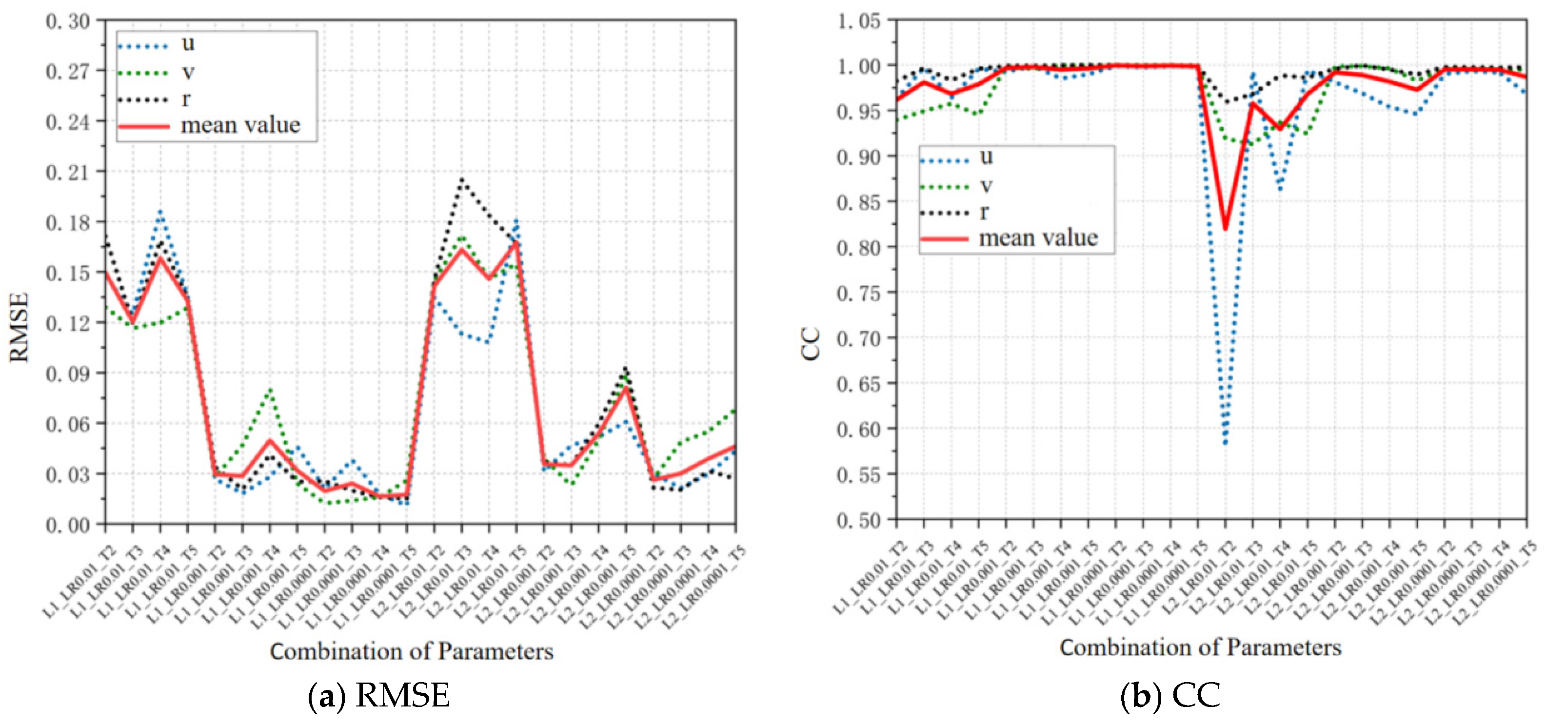
4.2. Discussion of Training Settings

Once the neural network structure is determined, the prediction accuracy is significantly influenced by the training settings. The following discussion covers several aspects of network training settings, including learning rate adjustment for the LSTM network (initial learning rate), training batch size, and window function width.

The following discussion covers the impact of different initial learning rates and window function widths on the two network configurations, as Figure 5 shows.

(1)

Learning Rate:

In both single-layer and double-layer networks, the worst performance was observed when the initial learning rate was set to 0.01. As the learning rate gradually decreased to 0.0001, network performance improved, reaching its best state with LR = 0.0001, demonstrating excellent prediction performance and strong correlation. Setting the initial learning rate too high can lead to rapid convergence, missing the optimal solution, or even causing unstable training.

(2)

Window Function Width:

When LR = 0.0001, the prediction accuracy of the single-layer network remained stable across different window function widths, maintaining excellent prediction accuracy. The best performance was achieved at T = 4, with RMSE reduced to 0.01649 and CC increased to 0.99931. Conversely, in the double-layer network, when LR = 0.001 or 0.0001, prediction accuracy was negatively correlated with the window function width, with RMSE increasing and CC decreasing. Increasing the window width in the LSTM double-layer network may lead to long-term dependency loss and gradient vanishing, reducing prediction accuracy. In contrast, the single-layer network was less affected, being simpler in structure with fewer parameters, making it easier to train and optimize.

To compare the appropriate window function width for the single-layer network, the training time for different window function widths can be observed in Figure 6.

Comparative analysis reveals that the model configuration with a total network layer count of 6, an LSTM network layer count of 1, 64 neurons, and a dropout regularization rate of 0.15—trained using a 5-fold cross-validation with a batch size of 32, an Adam optimizer with a learning rate of 0.0001, and a window function width of 2—exhibited the best performance in terms of RMSE and CC. The resulting RMSE was close to zero and the CC was close to 1, indicating that this model possesses excellent learning and generalization capabilities, making it highly suitable for subsequent ship maneuverability prediction tasks. Figure 7 shows the network parameters and structure of the optimized LSTM model.

4.3. Comparing Simulations

Based on the optimized LSTM structure, the motion prediction model was trained using sample data. The trained LSTM model was then applied to the validation set under wave conditions, comparing simulations based on the MMG model with those based on the LSTM black-box model. The validation set included both a 20°/20° zigzag test (as shown in Figure 8) and a 35° turning test (as shown in Figure 9), representing two of the most distinct maneuvering scenarios for USVs, neither of which were present in the training or testing datasets, ensuring the accuracy of generalization validation.

The comparison of simulations under wave disturbances for the two validation sets reveals that the predictions from the LSTM black-box model closely match the simulation results from the MMG model. This indicates that the black-box model constructed using the LSTM network demonstrates excellent learning and generalization capabilities. Despite the presence of complex noise distribution in the sample data and the loss of some data, the data preprocessing steps effectively repaired these deficiencies. Then, the LSTM neural network structure learned information from this data, with the forget gate playing a crucial role in filtering out disturbances in the sample data, thereby retaining essential information in the neural network that provides valuable insights for the model.

5. Conclusions

There is a logical challenge in applying simulation data to USV motion model identification, as the simulated data is often overly perfect, lacking noise and sampling loss issues. This results in machine learning algorithms easily capturing the features of the sample set but producing models with poor generalization, making them difficult to apply to other scenarios or in real-world situations. In response to this challenge, this paper addresses the identification of USV motion prediction models by developing an offline prediction model using machine learning methods. A simulation data processing method based on OU noise and the HMM is proposed, which brings the sample data closer to experimental data, which is characterized by random noise and random data loss. Subsequently, a sample data preprocessing strategy that includes MaxAbsScaler normalization, Kalman filtering and RRF smoothing, and Lagrange interpolation is proposed. This preprocessing allows the sample data to be effectively used in subsequent machine learning training. Following this, a 3-DOF black-box prediction model for USV maneuvering based on LSTM networks is established. The research then conduct a thorough comparative study of the LSTM-based black-box prediction model across three aspects: prediction accuracy, computational speed, and the complexity of parameter tuning. Based on the comparison results, an optimized selection strategy is proposed and proceeded with model training. Finally, the trained black-box model is applied to two validation datasets under different operating conditions, demonstrating the effectiveness and robustness of the proposed method. The findings of this research can be utilized in actual USV operations, where real-time navigation data can be used to train the USV maneuvering prediction model. This model can then be employed in model-based control systems, such as Model Predictive Control (MPC), to achieve stable USV navigation in complex environments. In this study, the focus was on offline modeling and prediction of USV maneuvering data. Future research should emphasize the utilization of real-time data for rapid, online, real-time training.

References

1. Wang, S. Research on development status and combat applications of USVs in worldwide. Command. Syst. 2019, 44, 11–15. [Google Scholar]
2. Yuan, X.Y. Hierarchical model identification method for unmanned surface vehicle. J. Shanghai Univ. (Nat. Sci.) 2020, 26, 896–908. [Google Scholar]
3. Abkowitz, M.A. Measurement of hydrodynamic characteristics from ship maneuvering trials by system identification. Trans. Soc. Nav. Archit. Mar. Eng. 1980, 88, 283–318. [Google Scholar]
4. Liu, Y.; Zou, L.; Zou, Z.; Guo, H.P. Predictions of ship maneuverability based on virtual captive model tests. Eng. Appl. Comput. Fluid Mech. 2018, 12, 334–353. [Google Scholar] [CrossRef]
5. Xu, H.; Soares, C.G. Hydrodynamic coefficient estimation for ship manoeuvring in shallow water using an optimal truncated LS-SVM. Ocean Eng. 2019, 191, 106488. [Google Scholar] [CrossRef]
6. He, H.; Wang, Z.; Zou, Z.; Liu, Y. System Identification Based on Completely Connected Neural Networks for Black-Box Modeling of Ship Maneuvers. In Advances in Guidance, Navigation and Control; Lecture Notes in Electrical Engineering; Springer: Singapore, 2022; Volume 644. [Google Scholar] [CrossRef]
7. Zhang, X.; Zou, Z. Identification of models of ship manoeuvring motion using Support Vector Regression and Particle Swarm Optimization. J. Ship Mech. 2016, 20, 1427–1432. [Google Scholar] [CrossRef]
8. Xu, H.; Hinostroza, M.A.; Wang, Z.; Guedes Soares, C. Experimental investigation of shallow water effect on vessel steering model using system identification method. Ocean Eng. 2020, 199, 106940. [Google Scholar] [CrossRef]
9. Xu, H.; Hassani, V.; Soares, C.G. Uncertainty analysis of the hydrodynamic coefficients estimation of a nonlinear manoeu-vring model based on planar motion mechanism tests. Ocean Eng. 2019, 173, 450–459. [Google Scholar] [CrossRef]
10. Pandey, J.; Hasegawa, K. Study on turning manoeuvre of catamaran surface vessel with a combined experimental and simulation method. IFAC-PapersOnLine 2016, 49, 446–451. [Google Scholar] [CrossRef]
11. Luo, W.; Zhang, Z. Modeling of ship maneuvering motion using neural networks. J. Mar. Sci. Appl. 2016, 15, 426–432. [Google Scholar] [CrossRef]
12. Carrillo, S.; Contreras, J. Obtaining first and second order nomoto models of a fluvial support patrol using identification techniques. Ship Sci. Technol. 2018, 11, 19–28. [Google Scholar] [CrossRef]
13. Liu, C.D.; Zhang, H.; Han, Y.; Shi, C. Black-box modeling and prediction of ship maneuverability based on Least Square Support Vector Machine. J. Ship Mech. 2013, 17, 872–877. [Google Scholar] [CrossRef]
14. Xu, F.; Chen, Q.; Zhou, Z. Modeling of Underwater Vehicles’ Maneuvering Motion by Using Integral Sample Structure for Identification. J. Ship Mech. 2014, 211–220. [Google Scholar]
15. Bonci, M.; Viviani, M.; Broglia, R.; Dubbioso, G. Method for estimating parameters of practical ship manoeuvring models based on the combination of RANSE computations and System Identification. Appl. Ocean Res. 2015, 52, 274–294. [Google Scholar] [CrossRef]
16. Gupta, P.; Rasheed, A.; Steen, S. Ship performance monitoring using machine-learning. Ocean Eng. 2022, 254, 111094. [Google Scholar] [CrossRef]
17. Zhang, Y.Y.; Wang, Z.H.; Zou, Z.J. Black-box modeling of ship maneuvering motion based on multi-output nu-support vector regression with random excitation signal. Ocean Eng. 2022, 257, 111279. [Google Scholar] [CrossRef]
18. Song, L.; Hao, L.; Tao, H.; Xu, C.; Guo, R.; Li, Y.; Yao, J. Research on Black-Box Modeling Prediction of USV Maneuvering Based on SSA-WLS-SVM. J. Mar. Sci. Eng. 2023, 11, 324. [Google Scholar] [CrossRef]
19. He, H.; Zou, Z. Black-Box Modeling of Ship Maneuvering Motion Using System Identification Method Based on BP Neural Network. In Proceedings of the ASME 2020 39th International Conference on Ocean, Offshore and Arctic Engineering, Virtual, Online, 3–7 August 2020; Volume 6B: Ocean Engineering. [Google Scholar] [CrossRef]
20. Liu, Y.; Xue, Y.; Huang, S.; Xue, G.; Jing, Q. Dynamic Model Identification of Ships and Wave Energy Converters Based on Semi-Conjugate Linear Regression and Noisy Input Gaussian Process. J. Mar. Sci. Eng. 2021, 9, 194. [Google Scholar] [CrossRef]
Figure 1. Model of the USV.
Jmse 12 01661 g001
Figure 2. USV motion prediction model based on LSTM.
Jmse 12 01661 g002
Figure 3. Impact of Network Structure on Prediction (the mean represents the average value of the corresponding parameter).
Jmse 12 01661 g003
Figure 4. Impact of Network Structure on Training Time.
Jmse 12 01661 g004
Figure 5. Impact of Training Settings on Prediction Performance.
Jmse 12 01661 g005
Figure 6. Impact of training parameters on Training Time.
Jmse 12 01661 g006
Figure 7. The network parameters and structure of the optimized LSTM model.
Jmse 12 01661 g007
Figure 8. Comparison of motion prediction results for the 20°/20° zigzag test under wave conditions.
Jmse 12 01661 g008
Figure 9. Comparison of motion prediction results for the 35° turning test under wave conditions.
Jmse 12 01661 g009