Study on the Damage Evolution and Failure Mechanism of Floor Strata under Coupled Static-Dynamic Loading Disturbance

Abstract

In the field test, we found that the failure depth of the goaf floor strata tends to be further because the periodic breaking and caving of the immediate roof, upper roof, and roof key stratum has dynamic stress disturbance effects on the floor. To further analyze its formation mechanism, this paper studies the damage evolution and fracture mechanism of goaf floor rock under the coupled static-dynamic loading disturbance caused by roof caving, based on the stress distribution state, the damage evolution equation of coal measure rock, the damage constitutive model, and the fracture criterion of floor rock. The main conclusions are listed as follows: 1. Based on the mining floor stress distribution, the floor beam model establishes the response mechanism of floor rock stress distribution. Also, the equation of stress distribution at any position in floor strata under mining dynamic load is given. 2. Combining the advantages of Bingham and the Generalized-Boydin model, the B-G damage constitutive model is established, which can describe the constitutive characteristics of coal measure rock under the coupled static-dynamic loading disturbance well. Furthermore, the variation law of parameters changing with strain rate is analyzed. 3. According to the twin-shear unified strength yield theory and the B-G damage constitutive model, coal measure rock’s twin-shear unified strength damage fracture criterion is established. Finally, the stress distribution expression of floor strata under concentrated and uniform dynamic loads is introduced, and the fracture criterion of goaf floor strata under a coupled static-dynamic loading disturbance is proposed.

1. Introduction

Energy is an essential material basis and a driving force for human civilization’s progress, which is also related to the national economy, people’s livelihoods, and national security. With the rapid development of China’s economy in recent years, the demand for energy has increased. China has become the largest energy consumer in the world [1]. Furthermore, in 2022, China’s energy consumption accounted for 26.4% of global energy consumption. Regarding the energy consumption structure, coal accounted for 55.4% [2]. Accordingly, the fundamental reality is that coal will occupy the dominant position in China’s energy consumption structure and will be difficult to change in the long run [3,4]. With the increasing depletion of high-grade coal resources in the shallow part and the rising coal mining intensity, mines gradually extend to deep coal seams with complex geological conditions. Therefore, the mining of deep coal seams faces more problems and challenges [5,6,7]. The deep rock mass is in a typical complex mechanical environment with high ground stress, high karst water pressure, high ground temperature, and strong mining disturbance [6,8,9]. Owing to the fact that the deep rock mechanical behavior is different from that of shallow rock and the mining intensity is increasing, the deep rock mass is in the limit equilibrium state, and the superposition coupling effect of dynamic and static stress fields under strong mining disturbance in the deep rock mass is apparent [10]. Moreover, the frequency, intensity, and scale of induced mine disasters are increasing, and the disaster mechanism is more complicated [11,12,13,14].

In terms of floor water hazard prevention in coal mining, the Permian coal seams in deep mining of North China-type coalfields are mostly karst water-filled deposits, which are mainly threatened by the tremendously thick Cambrian-Ordovician and Taiyuan formation karst limestone aquifer at the bottom of the coal seams [15,16]. The Cambrian-Ordovician karst is only a few meters to tens of meters away from the floor and can even be directly connected with the coal seam, with a high confined water level, rich water content, high head pressure, structural development of karst fissures and caves, and varied and complex geological conditions [17,18,19]. With the increase in mining depth and intensity, the floor rock mass is combined with high surrounding rock stress and strong dynamic and static stress superposition disturbances, leading to more damage and fractures in the impermeable layer and lower water resistance performance [6,10,20]. Therefore, the water inrush risk in deep high-intensity mining is significantly increased, and the floor water inrush disaster has become one of the most important factors restricting deep coal mining in China [15,16,21,22,23].

In the field measurement of many mining working faces, we found that in the working face advancing process, the periodic breaking and caving of the direct roof, the main roof, and the roof key strata have dynamic stress disturbance effects on the floor strata in the goaf. Therefore, the developing depth of water-conducting fractures in the goaf floor tends to deepen [24]. This mining geological phenomenon will increase the possibility of a lagging water inrush from the goaf floor. Thus, from field detection, similar simulation, numerical calculation, etc., the roof caving dynamic stress mechanism on floor failure and water inrush is studied in detail [24,25,26]. The research proves that the floor strata are not only affected by the static load but also by the dynamic stress disturbance caused by the impact force of the roof falling and the mine earthquake. The mining dynamic stress disturbance not only induces the occurrence of water inrush disasters but also plays a vital role in the breeding and development progress of water inrush disasters [26,27,28,29]. Especially for deep mining, the rock mass is more sensitive to the impact of dynamic stress disturbances under high static loads. As a result, simply considering the floor rock mass damage and failure caused by static load and the water inrush disaster induced by fracture activation cannot fully explain the complex mechanical problems in deep mining [10,30,31,32,33]. Overall, this paper takes the floor rock mass of deep mining as the research object and the collapse of the large roof area as the typical dynamic stress disturbance inducement. Moreover, based on the floor stress distribution under the superposition disturbance of mining dynamic and static load, the damage evolution equation of coal measure rock, the damage constitutive model, and the fracture criterion of the floor rock, this paper studies the damage evolution and fracture mechanism of the goaf floor strata under the superposition disturbance of mining dynamic and static load. The solutions are of great value to clarify the failure and water inrush mechanism of the floor fractured rock mass under the superposition disturbance of dynamic and static stress in deep high-intensity mining, the secondary failure mechanism of the floor fractured rock mass caused by strong mining disturbance in a high-stress environment, and the engineering mechanics characteristics of the floor fractured rock mass under the superposition disturbance of dynamic and static stress fields and seepage multi-field coupling effects.

2. The Floor Strata Stress Distribution under Mining Dynamic Load Disturbance

2.1. The Initial Stress Distribution of Floor Strata in Stope

2.1.1. The Support Pressure Distribution State of the Floor Strata

The support pressure of floor strata changes with the advancement of the working face, influencing the floor stress distribution. The influence of mining dynamic stress on the floor stress distribution is generated on the basis of its original stress distribution state. Therefore, this paper first analyzes the floor stress distribution under the support pressure of the working face. According to current research, the support pressure distribution of floor strata is shown in Figure 1 [34].

Taking the X-X axial section-plane (X-X section-plane), the distribution law of support pressure parallel to the working face can be analyzed. Thus, we can explore the floor’s original stress distribution characteristics on the transverse surface. The support pressure distribution of the X-X axial section plane is shown in Figure 2.

Taking the Y-Y axial section-plane (Y-Y section-plane), the distribution law of support pressure vertical to the working face can be analyzed. Then, the original floor stress distribution characteristics in the longitudinal plane can be analyzed. Without considering the support pressure generated by the hydraulic prop, the floor support pressure distribution of the Y-Y axial section plane is shown in Figure 3.

2.1.2. The Floor Strata Original Stress Distribution

According to the normal force on the boundary of the half-plane body (Figure 4), the stress component is obtained (Equation (1)).

$$\begin{array}{l}{\sigma }_{\rho }=-\frac{2F}{\pi }\frac{\cos \alpha }{\rho }\\ {\sigma }_{\alpha }=0\\ {\tau }_{\rho \alpha }={\tau }_{\alpha \rho }=0\end{array},$$

(1)

Using Equation (2) to change Equation (1) into a stress component in a rectangular coordinate, Equation (3) is obtained:

$$\begin{array}{l}{\sigma }_x={\sigma }_{\rho }{\cos }^2\alpha +{\sigma }_{\alpha }{\sin }^2\alpha -2{\tau }_{\rho \alpha }\sin \alpha \cos \alpha \\ {\sigma }_y={\sigma }_{\rho }{\sin }^2\alpha +{\sigma }_{\alpha }{\cos }^2\alpha +2{\tau }_{\rho \alpha }\sin \alpha \cos \alpha \\ {\tau }_{xy}=({\sigma }_{\rho }-{\sigma }_{\alpha })\sin \alpha \cos \alpha +{\tau }_{\rho \alpha }({\cos }^2\alpha -{\sin }^2\alpha )\end{array},$$

(2)

$$\begin{array}{l}{\sigma }_x=-\frac{2F}{\pi }\frac{{\cos }^3\alpha }{\rho }\\ {\sigma }_y=-\frac{2F}{\pi }\frac{{\sin }^2\alpha \cos \alpha }{\rho }\\ {\tau }_{xy}=-\frac{2F}{\pi }\frac{\sin \alpha {\cos }^2\alpha }{\rho }\end{array}.$$

(3)

By replacing Equation (3) with Equation (4), which is a rectangular coordinate and polar coordinate transformation formula, Equation (5) of the normal force on the boundary of the lower half-plane body in the rectangular coordinate system is obtained:

$$\begin{array}{cc}x=\rho \cos \alpha & y=\rho \sin \alpha \end{array}$$

(4)

$$\begin{array}{l}{\sigma }_x=-\frac{2F}{\pi }\frac{x^3}{{\left(x^2+y^2\right)}^2}\\ {\sigma }_y=-\frac{2F}{\pi }\frac{x{y}^2}{{\left(x^2+y^2\right)}^2}\\ {\tau }_{xy}=-\frac{2F}{\pi }\frac{x^{2}y}{{\left(x^2+y^2\right)}^2}\end{array}.$$

(5)

With the stress formula of the half-plane body boundary under the action of the normal concentrated force, the stress formula under the action of the normal distributed force can be obtained by the superposition principle. As shown in Figure 5, the half-plane is subjected to a distributed force on a boundary section. Where q is the load intensity at each point. Moreover, to calculate the stress at point M in the half plane, the coordinates of point M are set as (x, y). We take a micro-length $d\xi$ on the AB section, where the distance from the origin of coordinate O is $\xi$. The force $dF=qd\xi$ on it is regarded as a small, concentrated force, which can be obtained by Equation (5).

$$\begin{array}{l}d{\sigma }_x=-\frac{2qd\xi }{\pi }\frac{x^3}{{\left[x^2+{\left(y-\xi \right)}^2\right]}^2}\\ d{\sigma }_y=-\frac{2qd\xi }{\pi }\frac{x{\left(y-\xi \right)}^2}{{\left[x^2+{\left(y-\xi \right)}^2\right]}^2}\\ d{\tau }_{xy}=-\frac{2qd\xi }{\pi }\frac{x^2\left(y-\xi \right)}{{\left[x^2+{\left(y-\xi \right)}^2\right]}^2}\end{array}.$$

(6)

In order to obtain the floor strata stress state caused by all distributed forces, it is only necessary to superimpose the stresses caused by all small, concentrated forces. Therefore, we can get the integral of Equation (6).

$$\begin{array}{l}{\sigma }_x=-\frac{2}{\pi }{\displaystyle {\int }_{-b}^a\frac{q{x}^{3}d\xi }{{\left[x^2+{\left(y-\xi \right)}^2\right]}^2}}\\ {\sigma }_y=-\frac{2}{\pi }{\displaystyle {\int }_{-b}^a\frac{qx{\left(y-\xi \right)}^{2}d\xi }{{\left[x^2+{\left(y-\xi \right)}^2\right]}^2}}\\ {\tau }_{xy}=-\frac{2}{\pi }{\displaystyle {\int }_{-b}^a\frac{q{x}^2\left(y-\xi \right)d\xi }{{\left[x^2+{\left(y-\xi \right)}^2\right]}^2}}\end{array}.$$

(7)

The Original Stress Distribution of Floor Strata in the X-X Axial Section Plane

The stress distribution of the X-X axis section taken from the working face indicates that the support pressure on the floor is symmetrical along the central axis. Furthermore, the nonlinear support pressure is simplified to a linear support pressure. Thus, the support pressure distribution of the floor strata on the X-X axis section can be simplified, as shown in Figure 6.

As shown in Figure 6, $\gamma h$ is the overburden pressure of floor strata, $k$ is the stress intensity factor. According to the elastic mechanics theory, the floor stress distribution state under the effect of support pressure can be derived.

First, the support pressure in Figure 6 can be expressed as follows:

$$q(\xi )=\left\{\begin{array}{ll}0& 0\le \xi <x_a\\ \frac{k\gamma h}{l_2}(\xi -l_1)& x_a\le \xi <x_b\\ \frac{(1-k)\gamma h}{l_3}(\xi -l_1-l_2)+k\gamma h& x_b\le \xi <x_c\\ \gamma h& x_c\le \xi <x_d\end{array}\right..$$

(8)

According to Equations (7) and (8), we can obtain the stress distribution expression of floor strata (X-X plane):

$$\begin{array}{l}{\sigma }_x=-\frac{2}{\pi }{\displaystyle {\int }_0^{x_d}\frac{q(\xi )x^{3}d\xi }{{\left[x^2+{\left(y-\xi \right)}^2\right]}^2}}\\ =-\frac{2}{\pi }\gamma h\left\{\begin{array}{l}{\displaystyle {\int }_{x_a}^{x_b}\frac{k(\xi -l_1)x^{3}d\xi }{l_2{\left[x^2+{\left(y-\xi \right)}^2\right]}^2}}\\ +{\displaystyle {\int }_{x_b}^{x_c}\frac{[(1-k)(\xi -l_1-l_2)+k{l}_3]x^{3}d\xi }{l_3{\left[x^2+{\left(y-\xi \right)}^2\right]}^2}+{\displaystyle {\int }_{x_c}^{x_d}\frac{x^{3}d\xi }{{\left[x^2+{\left(y-\xi \right)}^2\right]}^2}}}\end{array}\right\}\end{array},$$

(9)

$$\begin{array}{l}{\sigma }_y=-\frac{2}{\pi }{\displaystyle {\int }_0^{x_d}\frac{q(\xi )x{\left(y-\xi \right)}^{2}d\xi }{{\left[x^2+{\left(y-\xi \right)}^2\right]}^2}}\\ =-\frac{2}{\pi }\gamma h\left\{\begin{array}{l}{\displaystyle {\int }_{x_a}^{x_b}\frac{k(\xi -l_1)x{\left(y-\xi \right)}^{2}d\xi }{l_2{\left[x^2+{\left(y-\xi \right)}^2\right]}^2}}\\ +{\displaystyle {\int }_{x_b}^{x_c}\frac{[(1-k)(\xi -l_1-l_2)+l_{3}k]x{\left(y-\xi \right)}^{2}d\xi }{l_3{\left[x^2+{\left(y-\xi \right)}^2\right]}^2}+{\displaystyle {\int }_{x_c}^{x_d}\frac{x{\left(y-\xi \right)}^{2}d\xi }{{\left[x^2+{\left(y-\xi \right)}^2\right]}^2}}}\end{array}\right\}\end{array},$$

(10)

$$\begin{array}{l}{\tau }_{xy}=-\frac{2}{\pi }{\displaystyle {\int }_0^{x_d}\frac{q(\xi )x^2\left(y-\xi \right)d\xi }{{\left[x^2+{\left(y-\xi \right)}^2\right]}^2}}\\ =-\frac{2}{\pi }\gamma h\left\{\begin{array}{l}{\displaystyle {\int }_{x_a}^{x_b}\frac{k(\xi -l_1)x^2\left(y-\xi \right)d\xi }{l_2{\left[x^2+{\left(y-\xi \right)}^2\right]}^2}}\\ +{\displaystyle {\int }_{x_b}^{x_c}\frac{[(1-k)(\xi -l_1-l_2)+k{l}_3]x^2\left(y-\xi \right)d\xi }{l_3{\left[x^2+{\left(y-\xi \right)}^2\right]}^2}+{\displaystyle {\int }_{x_c}^{x_d}\frac{x^2\left(y-\xi \right)d\xi }{{\left[x^2+{\left(y-\xi \right)}^2\right]}^2}}}\end{array}\right\}\end{array}.$$

(11)

The Original Stress Distribution of Floor Strata in the Y-Y Axial Section Plane

Regarding the Y-Y axis section taken from the working face, the nonlinear support pressure can be approximately simplified to linear support pressure. Thus, the support pressure distribution of the floor strata on the Y-Y axis section can be simplified, as shown in Figure 7.

The support pressure in Figure 7 can be expressed as follows:

$$q\left(\xi \right)=\left\{\begin{array}{cc}\gamma h\hfill & 0\le \xi <x_a\hfill \\ \frac{\gamma h}{l_2}\left(l_1+l_2-\xi \right)\hfill & x_a\le \xi <x_b\hfill \\ 0\hfill & x_b\le \xi <x_c\hfill \\ \frac{k\gamma h}{l_4}\left(\xi -l_1-l_2-l_3\right)\hfill & x_c\le \xi <x_d\hfill \\ \frac{(1-k)\gamma h}{l_5}\left(\xi -l_1-l_2-l_3-l_4\right)+k\gamma h\hfill & x_d\le \xi <x_e\\ \gamma h\hfill & x_e\le \xi <x_f\hfill \end{array}.\right.$$

(12)

Based on Equations (7) and (12), we can obtain the stress distribution expression of floor strata (Y-Y plane):

$$\begin{array}{c}{\sigma }_x=-\frac{2}{\pi }{\int }_0^{x_f}\frac{q\left(\xi \right)x^{3}d\xi }{{\left[x^2+{(y-\xi )}^2\right]}^2}\hfill \\ =-\frac{2}{\pi }\gamma h\left\{\begin{array}{c}{\int }_0^{x_a}\frac{x^{3}d\xi }{{\left[x^2+{(y-\xi )}^2\right]}^2}+{\int }_{x_a}^{x_b}\frac{\left(l_1+l_2-\xi \right)x^{3}d\xi }{l_2{\left[x^2+{(y-\xi )}^2\right]}^2}+{\int }_{x_c}^{x_d}\frac{k\left(\xi -l_1-l_2-l_3\right)x^{3}d\xi }{l_4{\left[x^2+{(y-\xi )}^2\right]}^2}\hfill \\ +{\int }_{x_d}^{x_e}\left[(1-k)\left(\xi -l_1-l_2-l_3-l_4\right)+l_{5}k\right]\frac{x^{3}d\xi }{l_5{\left[x^2+{(y-\xi )}^2\right]}^2}+{\int }_{x_e}^{x_f}\frac{x^{3}d\xi }{{\left[x^2+{(y-\xi )}^2\right]}^2}\hfill \end{array}\right\},\hfill \end{array}$$

(13)

$$\begin{array}{c}{\sigma }_y=-\frac{2}{\pi }{\int }_0^{x_d}\frac{q\left(\xi \right)x{(y-\xi )}^{2}d\xi }{{\left[x^2+{(y-\xi )}^2\right]}^2}\hfill \\ =-\frac{2}{\pi }\gamma h\left\{\begin{array}{c}{\int }_0^{x_a}\frac{x{(y-\xi )}^{2}d\xi }{{\left[x^2+{(y-\xi )}^2\right]}^2}+{\int }_{x_d}^{x_b}\frac{\left(l_1+l_2-\xi \right)x{(y-\xi )}^{2}d\xi }{l_2{\left[x^2+{(y-\xi )}^2\right]}^2}+{\int }_{x_e}^{x_d}\frac{k\left(\xi -l_1-l_2-l_3\right)x{(y-\xi )}^{2}d\xi }{l_4{\left[x^2+{(y-\xi )}^2\right]}^2}\hfill \\ +{\int }_{x_d}^{x_x}\left[(1-k)\left(\xi -l_1-l_2-l_3-l_4\right)+l_{5}k\right]\frac{x{(y-\xi )}^{2}d\xi }{l_5{\left[x^2+{(y-\xi )}^2\right]}^2}+{\int }_{x_e}^{x_f}\frac{x{(y-\xi )}^{2}d\xi }{{\left[x^2+{(y-\xi )}^2\right]}^2}\hfill \end{array}\right\}\hfill \end{array},$$

(14)

$$\begin{array}{c}{\tau }_{xy}=-\frac{2}{\pi }{\int }_0^{x_d}\frac{q\left(\xi \right)x^2(y-\xi )d\xi }{{\left[x^2+{(y-\xi )}^2\right]}^2}\hfill \\ =-\frac{2}{\pi }\gamma h\left\{\begin{array}{c}{\int }_0^{x_a}\frac{x^2(y-\xi )d\xi }{{\left[x^2+{(y-\xi )}^2\right]}^2}+{\int }_{x_a}^{x_b}\frac{\left(l_1+l_2-\xi \right)x^2(y-\xi )d\xi }{l_2{\left[x^2+{(y-\xi )}^2\right]}^2}+{\int }_{x_c}^{x_d}\frac{k\left(\xi -l_1-l_2-l_3\right)x^2(y-\xi )d\xi }{l_4{\left[x^2+{(y-\xi )}^2\right]}^2}\hfill \\ +{\int }_{x_d}^{x_e}\left[(1-k)\left(\xi -l_1-l_2-l_3-l_4\right)+l_{5}k\right]\frac{x^2(y-\xi )d\xi }{l_5{\left[x^2+{(y-\xi )}^2\right]}^2}+{\int }_{x_e}^{x_f}\frac{x^2(y-\xi )d\xi }{{\left[x^2+{(y-\xi )}^2\right]}^2}\hfill \end{array}\right\}\hfill \end{array}.$$

(15)

2.2. Response Mechanism of Floor Surrounding Rock Stress Distribution under Mining Dynamic Load

2.2.1. Floor Equivalent Static Load Analysis under Dynamic Load

The influence of mining dynamic load on floor strata mainly comes from the dynamic load impact of the roof and overlying stratum breaking and caving on the floor. According to the actual situation on site, the forms of roof fracture and collapse can be divided into broken collapse and integral collapse. Thus, the roof and overlying strata are simplified into a beam model, and the above two collapse forms are shown in Figure 8.

From the perspective of the Y-Y plane, Figure 8a shows the fractured caving model of the middle and ends of the roof strata, which has a great impact load and strong collapsing force in local parts. Moreover, the dynamic load impact force on the floor surface is a concentrated force distribution. In addition, Figure 8b illustrates the roof integral collapse model from the Y-Y plane perspective, which has large dynamic impact loads and great influences on the floor, resulting in strong destructive power. The dynamic load impact force on the floor surface can be seen as a uniform force distribution.

Through the simplification of the model, the load on the floor contact surface, line, and point is obtained when the roof is broken and collapsed, which is used as the boundary load condition for solving the stress distribution of the floor and the underlying strata.

As shown in Figure 9, the cross-section (Y-Y plane) along the floor mining direction is simplified as a two-end clamped beam structure, and the impact load is solved by the engineering mechanics method.

According to the energy method, the rock dynamic load coefficient is listed as Equation (16) when the floor is subjected to an impact load.

$$K_d=1+\sqrt{1+\frac{2H}{{\Delta }_{st}}}.$$

(16)

where H is the roof strata falling height, and ${\Delta }_{st}$ is the deflection of the beam under static load.

• Based on related material mechanics theories, when the floor is under the concentrated dynamic load F, the static load deflection at beam C caused by static load F is listed as Equation (17).

  $${\Delta }_{st}=\frac{F{a}^3{\left(l-a\right)}^3}{3EI{l}^3}.$$

  (17)

Taking Equation (17) into Equation (16), we can obtain the actual dynamic load on the floor (Equation (18)).

$$F_{\mathrm{d}}=K_{d}F=F+F\sqrt{1+\frac{6EIH{l}^3}{F{a}^3{\left(l-a\right)}^3}}.$$

(18)

• Similarly, according to the related material mechanics and structural mechanics theories, when the floor is under the effect of uniform dynamic load q, as shown in Figure 9, the static load deflection at beam b caused by static load q is $\left.w(x)\right|x\in (a,a+b)$. Thus, the rock dynamic load coefficient is presented as Equation (19).

  $$K_d=\left.1+\sqrt{1+\frac{2H}{w(x)}}\right|x\in (a,a+b).$$

  (19)

From Equation (19), we can obtain the uniform dynamic load on the floor (Equation (20)).

$$q_{\mathrm{d}}=K_{d}q=(\left.1+\sqrt{1+\frac{2H}{w(x)}})q\right|x\in (a,a+b),$$

(20)

where the expression of $w(x)$ is listed as follows:

$$w(x)=\frac{1}{EI}[\frac{1}{2}(M_1+F_{1}l)x^2-\frac{1}{6}{F}_1{x}^3-\frac{q}{24}{(a+b-x)}^4+Ax+B],$$

(20a)

$$A=-\frac{q{b}^3}{24}-\frac{qb}{2}{(a+\frac{b}{2})}^2,$$

(20b)

$$B=\frac{q{b}^3}{24}(\frac{b}{2}+1)+\frac{qb}{2}{(a+\frac{b}{2})}^2[\frac{a}{3}+\frac{b}{6}+1],$$

(20c)

$$F_1=\frac{q}{l^2}[{(a+b)}^3-a^3]-\frac{3q}{2l^3}[{(a+b)}^4-a^4]+\frac{2q}{l^3}[{(a+b)}^3(l-a-b)-a^3(l-a)],$$

(20d)

$$M_1=\frac{3q}{4l^2}[{(a+b)}^4-a^4]-\frac{q}{l^2}[{(a+b)}^3(l-a-b)-a^3(l-a)]-\frac{2q}{3l}[{(a+b)}^3-a^3].$$

(20e)

2.2.2. Stress Response of Floor Surrounding Rock under Dynamic Load

Concentrated Dynamic Load

According to the above hypothesis, when the roof and overlying strata collapse in the middle and end, the response to the floor stress is superimposed by the response of the original support force and the concentrated dynamic load. Therefore, the boundary load of floor strata can be illustrated in Figure 10.

The concentrated dynamic load is listed as Equation (21).

$$F_{\mathrm{d}}=\left[1+\sqrt{1+\frac{6EIH{({\displaystyle {\displaystyle \sum _{i=1}^7}{l}_1})}^3}{F{({\displaystyle {\displaystyle \sum _{i=4}^7}{l}_1})}^3{\left({\displaystyle {\displaystyle \sum _{i=1}^3}{l}_1}\right)}^3}}\right]P,$$

(21)

where P is the weight of the collapsing rock and H is the roof falling height (coal mining thickness).

Equation (22) shows the stress response of the floor stress distribution state to the concentrated dynamic load.

$$\begin{array}{l}{\sigma }_{F_{d}x}=-\frac{2F_{\mathrm{d}}}{\pi }\frac{{(x-{\displaystyle {\displaystyle \sum _{i=1}^3}{l}_1})}^3}{{\left({(x-{\displaystyle {\displaystyle \sum _{i=1}^3}{l}_1})}^2+y^2\right)}^2}\\ {\sigma }_{F_{d}y}=-\frac{2F_{\mathrm{d}}}{\pi }\frac{(x-{\displaystyle {\displaystyle \sum _{i=1}^3}{l}_1})y^2}{{\left({(x-{\displaystyle {\displaystyle \sum _{i=1}^3}{l}_1})}^2+y^2\right)}^2}\\ {\tau }_{F_{d}xy}=-\frac{2F_{\mathrm{d}}}{\pi }\frac{{(x-{\displaystyle {\displaystyle \sum _{i=1}^3}{l}_1})}^{2}y}{{\left({(x-{\displaystyle {\displaystyle \sum _{i=1}^3}{l}_1})}^2+y^2\right)}^2}\end{array}.$$

(22)

Therefore, the stress response expression of the concentrated dynamic load and the original roof support force on the floor strata is expressed as follows:

$$\begin{array}{c}{\sigma }_x=-\frac{2}{\pi }{\int }_0^{x_{\mathrm{g}}}\frac{q\left(\xi \right)x^{3}d\xi }{{\left[x^2+{(y-\xi )}^2\right]}^2}+{\sigma }_{F_{d}x}\hfill \\ =-\frac{2}{\pi }\gamma h\left\{\begin{array}{c}{\int }_0^{x_a}\frac{x^{3}d\xi }{{\left[x^2+{(y-\xi )}^2\right]}^2}+{\int }_{x_a}^{x_b}\frac{\left({\displaystyle \sum _{i=1}^2}{l}_i-\xi \right)x^{3}d\xi }{l_2{\left[x^2+{(y-\xi )}^2\right]}^2}+{\int }_{x_d}^{x_e}\frac{k\left(\xi -{\displaystyle \sum _{i=1}^4}{l}_i\right)x^{3}d\xi }{l_5{\left[x^2+{(y-\xi )}^2\right]}^2}\hfill \\ +{\int }_{x_e}^{x_f}\left[(1-k)\left(\xi -{\displaystyle \sum _{i=1}^5}{l}_i\right)+l_{6}k\right]\frac{x^{3}d\xi }{l_6{\left[x^2+{(y-\xi )}^2\right]}^2}+{\int }_{x_f}^{x_g}\frac{x^{3}d\xi }{{\left[x^2+{(y-\xi )}^2\right]}^2}\hfill \end{array}\right\}\hfill \\ -\frac{2}{\pi }\frac{{\left(x-{\displaystyle \sum _{i=1}^3}{l}_i\right)}^3}{{\left({\left(x-{\displaystyle \sum _{i=1}^3}{l}_i\right)}^2+y^2\right)}^2}\left[1+\sqrt{1+\frac{6EIH{\left({\displaystyle \sum _{i=1}^7}{l}_i\right)}^3}{F{\left({\displaystyle \sum _{i=4}^7}{l}_i\right)}^3{\left({\displaystyle \sum _{i=1}^3}{l}_i\right)}^3}}\right]P\hfill \end{array}$$

(23)

$$\begin{array}{c}{\sigma }_y=-\frac{2}{\pi }{\int }_0^{x_{\mathrm{g}}}\frac{q\left(\xi \right)x{(y-\xi )}^{2}d\xi }{{\left[x^2+{(y-\xi )}^2\right]}^2}+{\sigma }_{F_{d}y}\hfill \\ =-\frac{2}{\pi }\gamma h\left\{\begin{array}{c}{\int }_0^{x_a}\frac{x{(y-\xi )}^{2}d\xi }{{\left[x^2+{(y-\xi )}^2\right]}^2}+{\int }_{x_a}^{x_{\mathrm{b}}}\frac{\left({\displaystyle \sum _{i=1}^2}{l}_i-\xi \right)x{(y-\xi )}^{2}d\xi }{l_2{\left[x^2+{(y-\xi )}^2\right]}^2}+{\int }_{x_{\mathrm{d}}}^{x_e}\frac{k\left(\xi -{\displaystyle \sum _{i=1}^4}{l}_i\right)x{(y-\xi )}^{2}d\xi }{l_5{\left[x^2+{(y-\xi )}^2\right]}^2}\hfill \\ +{\int }_{x_e}^{x_f}\left[(1-k)\left(\xi -{\displaystyle \sum _{i=1}^5}{l}_i\right)+l_{6}k\right]\frac{x{(y-\xi )}^{2}d\xi }{l_6{\left[x^2+{(y-\xi )}^2\right]}^2}+{\int }_{x_f}^{x_g}\frac{x{(y-\xi )}^{2}d\xi }{{\left[x^2+{(y-\xi )}^2\right]}^2}\hfill \end{array}\right\}\hfill \\ -\frac{2}{\pi }\frac{\left(x-{\displaystyle \sum _{i=1}^3}{l}_i\right)y^2}{{\left.{\left(x-{\displaystyle \sum _{i=1}^3}{l}_i\right)}^2+y^2\right)}^2}\left[1+\sqrt{1+\frac{6EIH{\left({\displaystyle \sum _{i=1}^7}{l}_i\right)}^3}{F{\left({\displaystyle \sum _{i=4}^7}{l}_i\right)}^3{\left({\displaystyle \sum _{i=1}^3}{l}_i\right)}^3}}\right]P\hfill \end{array}$$

(24)

$$\begin{array}{c}{\tau }_{xy}=-\frac{2}{\pi }{\int }_0^{x_{\mathrm{g}}}\frac{q\left(\xi \right)x^2(y-\xi )d\xi }{{\left[x^2+{(y-\xi )}^2\right]}^2}+{\tau }_{F_{d}xy}\hfill \\ =-\frac{2}{\pi }\gamma h\left\{\begin{array}{c}{\int }_0^{x_a}\frac{x^2(y-\xi )d\xi }{{\left[x^2+{(y-\xi )}^2\right]}^2}+{\int }_{x_a}^{x_b}\frac{\left({\displaystyle \sum _{i=1}^2}{l}_i-\xi \right)x^2(y-\xi )d\xi }{l_2{\left[x^2+{(y-\xi )}^2\right]}^2}+{\int }_{x_d}^{x_e}\frac{k\left(\xi -{\displaystyle \sum _{i=1}^4}{l}_i\right)x^2(y-\xi )d\xi }{l_5{\left[x^2+{(y-\xi )}^2\right]}^2}\hfill \\ +{\int }_{x_e}^{x_f}\left[(1-k)\left(\xi -{\displaystyle \sum _{i=1}^5}{l}_i\right)+l_{6}k\right]\frac{x^2(y-\xi )d\xi }{l_6{\left[x^2+{(y-\xi )}^2\right]}^2}+{\int }_{x_f}^{x_g}\frac{x^2(y-\xi )d\xi }{{\left[x^2+{(y-\xi )}^2\right]}^2}\hfill \end{array}\right\}\hfill \\ -\frac{2}{\pi }\frac{{\left(x-{\displaystyle \sum _{i=1}^3}{l}_i\right)}^{2}y}{{\left({\left(x-{\displaystyle \sum _{i=1}^3}{l}_i\right)}^2+y^2\right)}^2}\left[1+\sqrt{1+\frac{6EIH{\left({\displaystyle \sum _{i=1}^7}{l}_i\right)}^3}{F{\left({\displaystyle \sum _{i=4}^7}{l}_i\right)}^3{\left({\displaystyle \sum _{i=1}^3}{l}_i\right)}^3}}\right]P\hfill \end{array}$$

(25)

Uniform Dynamic Load

Based on the above hypothesis, when the roof and overlying strata collapse, the response to the floor stress is superimposed by the response of the original support force and the uniform dynamic load. Thus, the boundary load of floor strata can be illustrated in Figure 11.

The uniform dynamic load is expressed as Equation (26).

$$q_{\mathrm{d}}=(\left.1+\sqrt{1+\frac{2H}{w(x)}})q\right|x\in (c,d)=(\left.1+\sqrt{1+\frac{2H}{w(x)}})\gamma h_1\right|x\in (c,d).$$

(26)

where $h_1$ is the thickness of the roof and overlying strata collapsing.

Thus, the stress response expression of the uniformly distributed dynamic load and the original roof support force on the floor strata is listed as follows:

$$\begin{array}{c}{\sigma }_x=-\frac{2}{\pi }{\int }_0^{x_{\mathrm{h}}}\frac{q\left(\xi \right)x^{3}d\xi }{{\left[x^2+{(y-\xi )}^2\right]}^2}+{\sigma }_{F_{d}x}\hfill \\ =-\frac{2}{\pi }\gamma h\left\{\begin{array}{c}{\int }_0^{x_a}\frac{x^{3}d\xi }{{\left[x^2+{(y-\xi )}^2\right]}^2}+{\int }_{x_a}^{x_b}\frac{\left({\displaystyle \sum _{i=1}^2}{l}_i-\xi \right)x^{3}d\xi }{l_2{\left[x^2+{(y-\xi )}^2\right]}^2}+{\int }_{x_e}^{x_f}\frac{k\left(\xi -{\displaystyle \sum _{i=1}^5}{l}_i\right)x^{3}d\xi }{l_6{\left[x^2+{(y-\xi )}^2\right]}^2}\hfill \\ +{\int }_{x_f}^{x_g}\left[(1-k)\left(\xi -{\displaystyle \sum _{i=1}^6}{l}_i\right)+l_{7}k\right]\frac{x^{3}d\xi }{l_7{\left[x^2+{(y-\xi )}^2\right]}^2}+{\int }_{x_g}^{x_h}\frac{x^{3}d\xi }{{\left[x^2+{(y-\xi )}^2\right]}^2}\hfill \end{array}\right\},\hfill \\ -\frac{2}{\pi }{\int }_{x_{\mathrm{c}}}^{x_{\mathrm{d}}}\frac{(1+\sqrt{1+\frac{2H}{w\left(x\right)}})\gamma h_1{x}^{3}d\xi }{{\left[x^2+{(y-\xi )}^2\right]}^2}\hfill \end{array}$$

(27)

$$\begin{array}{c}{\sigma }_y=-\frac{2}{\pi }{\int }_0^{x_{\mathrm{g}}}\frac{q\left(\xi \right)x{(y-\xi )}^{2}d\xi }{{\left[x^2+{(y-\xi )}^2\right]}^2}+{\sigma }_{F_{d}y}\hfill \\ =-\frac{2}{\pi }\gamma h\left\{\begin{array}{c}{\int }_0^{x_a}\frac{x{(y-\xi )}^{2}d\xi }{{\left[x^2+{(y-\xi )}^2\right]}^2}+{\int }_{x_a}^{x_j}\frac{\left({\displaystyle \sum _{i=1}^2}{l}_i-\xi \right)x{(y-\xi )}^{2}d\xi }{l_2{\left[x^2+{(y-\xi )}^2\right]}^2}+{\int }_{x_e}^{x_f}\frac{k\left(\xi -{\displaystyle \sum _{i=1}^5}{l}_i\right)x{(y-\xi )}^{2}d\xi }{l_6{\left[x^2+{(y-\xi )}^2\right]}^2}\hfill \\ +{\int }_{x_f}^{x_g}\left[(1-k)\left(\xi -{\displaystyle \sum _{i=1}^6}{l}_i\right)+l_{7}k\right]\frac{x{(y-\xi )}^{2}d\xi }{l_7{\left[x^2+{(y-\xi )}^2\right]}^2}+{\int }_{x_g}^{x_h}\frac{x{(y-\xi )}^{2}d\xi }{{\left[x^2+{(y-\xi )}^2\right]}^2}\hfill \end{array}\right\}\hfill \\ -\frac{2}{\pi }{\int }_{x_c}^{x_{\mathrm{d}}}\frac{\left(1+\sqrt{1+\frac{2H}{w\left(x\right)}}\right)\gamma h_{1}x{(y-\xi )}^{2}d\xi }{{\left[x^2+{(y-\xi )}^2\right]}^2}\hfill \end{array}$$

(28)

$$\begin{array}{c}{\tau }_{xy}=-\frac{2}{\pi }{\int }_0^{x_{\mathrm{g}}}\frac{q\left(\xi \right)x^2(y-\xi )d\xi }{{\left[x^2+{(y-\xi )}^2\right]}^2}+{\tau }_{F_{d}xy}\hfill \\ =-\frac{2}{\pi }\gamma h\left\{\begin{array}{c}{\int }_0^{x_a}\frac{x^2(y-\xi )d\xi }{{\left[x^2+{(y-\xi )}^2\right]}^2}+{\int }_{x_a}^{x_b}\frac{\left({\displaystyle \sum _{i=1}^2}{l}_i-\xi \right)x^2(y-\xi )d\xi }{l_2{\left[x^2+{(y-\xi )}^2\right]}^2}+{\int }_{x_e}^{x_f}\frac{k\left(\xi -{\displaystyle \sum _{i=1}^5}{l}_i\right)x^2(y-\xi )d\xi }{l_6{\left[x^2+{(y-\xi )}^2\right]}^2}\hfill \\ +{\int }_{x_f}^{x_g}\left[(1-k)\left(\xi -{\displaystyle \sum _{i=1}^6}{l}_i\right)+l_{7}k\right]\frac{x^2(y-\xi )d\xi }{l_7{\left[x^2+{(y-\xi )}^2\right]}^2}+{\int }_{x_s}^{x_h}\frac{x^2(y-\xi )d\xi }{{\left[x^2+{(y-\xi )}^2\right]}^2}\hfill \end{array}\right\}\hfill \\ -\frac{2}{\pi }{\int }_{x_c}^{x_d}\frac{\left(1+\sqrt{1+\frac{2H}{w\left(x\right)}}\right)\gamma h_1{x}^2(y-\xi )d\xi }{{\left[x^2+{(y-\xi )}^2\right]}^2}\hfill \end{array}$$

(29)

3. Floor Surrounding Rock Damage Constitutive Model under the Dynamic Load Effect

3.1. Floor Rock Damage Evolution Model under Dynamic Load Effect

3.1.1. Common Rock Damage Evolution Model [35,36,37,38,39]

When the microcosmic element strength accords with normal distribution, the rock damage variables can be expressed as:

$$\varphi (\epsilon )=\frac{1}{S\sqrt{2\pi }}\exp \left[-\frac{1}{2}{(\frac{x-{\epsilon }_0}{S})}^2\right],$$

(30)

$$D={\displaystyle {\int }_0^{\epsilon }\frac{1}{S\sqrt{2\pi }}}\exp \left[-\frac{1}{2}{(\frac{x-{\epsilon }_0}{S})}^2\right]dx.$$

(31)

where ${\epsilon }_0$ and $S$ are respectively the mathematical expectation and mean square error of the normal distribution, $D$ is the damage variable, and $\varphi (\epsilon )$ is the normal distribution probability density function of material strength.

• When the microcosmic element strength obeys the Weibull distribution, the rock damage variable can be expressed as

$$\varphi (\epsilon )=\frac{m}{a}{\epsilon }^{m-1}\exp (-\frac{{\epsilon }^m}{a}),$$

(32)

$$D=1-\exp (-\frac{{\epsilon }^m}{a}).$$

(33)

where ${\epsilon }_0$ and $S$ are respectively the mathematical expectation and mean square error of the normal distribution, $D$ is the damage variable, and $\varphi (\epsilon )$ is the normal distribution probability density function of material strength.

• Tensile impact damage

Yang R. presented the rock damage model [36] under dynamic load in 1996 and defined the damage variable as follows:

$$D=1-\exp (-C_d^2),$$

(34)

$$d{C}_d/dt=\alpha {(\epsilon -{\epsilon }_c)}^{\beta }.$$

(35)

where $\alpha$ and $\beta$ are material constants, respectively, $D$ is the damage variable, and ${\epsilon }_c$ is the critical strain.

• Acoustic-wave-induced damage

Based on the rock dynamic load impact experiment, Gao et al. [37] defined the damage variable under impact load with wave velocity as follows:

$$D=1-{(c_{\mathrm{p}}/c_{\mathrm{p}0})}^2,$$

(36)

where $c_{\mathrm{p}}$ and $c_{\mathrm{p}0}$ are damaged and undamaged longitudinal wave velocity of rock materials.

• Rock damage under the impact load, considering temperature effects.

As illustrated by Equation (37), Li [38] obtained the damage evolution equation of coal measure sandstone under high temperature and high strain rate through the SHPB test of sandstone with high temperature.

$$D_{\epsilon T}=A(T){\epsilon }^2+B(T)\epsilon +C(T),$$

(37)

Also, the effects of the heating rate and the strain rate are shown in Equation (38).

$$D_{\dot{\epsilon }T}=A(\dot{\epsilon }){\epsilon }^2+B(\dot{\epsilon })\epsilon +C(\dot{\epsilon }),$$

(38)

$$D_{\epsilon \dot{T}}=A(\dot{T}){\epsilon }^2+B(\dot{T})\epsilon +C(\dot{T}).$$

(39)

where $\dot{\epsilon }$ and $\dot{T}$ are strain rate and heating rate, respectively.

• Fractional damage model

As shown in Equation (40), Li [40] introduced the fractal dimension into the definition of damage variables, and the definition of damage variable related to the fractal dimension is given as follows:

$$D=\frac{16}{9}\frac{1-{\nu }_e^2}{1-2{\nu }_e}\beta a_0^{3-D_f}.$$

(40)

where ${\nu }_e$ is equivalent poisson’s ratio, $\beta$ is grain shape correction coefficient, $a_0$ is average size of mineral grain, and $D_f$ is fractal dimension.

3.1.2. Rock Damage Evolution Model Considering Dynamic Strain Rate Effects

As a heterogeneous material, the rock contains many randomly distributed micro-defects, such as micro-cracks, holes, weakening surfaces, etc. Therefore, the failure of the rock microunit is also random under the load effect. Considering the complex effect of mining dynamic load on floor rock, statistical principles are used to study the effect of roof caving dynamic load on floor rock.

A traditional damage variable is usually defined by a certain variable change. For example, Rabotnov defined the damage variable as the effective cross section.

$$D=1-\frac{A_{\mathrm{ef}}}{A}.$$

(41)

where $D$ is the damage variable, $A_{\mathrm{ef}}$ is the effective action area, and A is the material initial cross-sectional area.

Lamaiter et al. used effective elastic modulus to define damage variables [41].

$$D=1-\frac{E^{\ast }}{E},$$

(42)

where $D$ is the damage variable, $E^{\ast }$ is the effective elastic modulus (the material elastic modulus during damage), and $E$ is the material initial elastic modulus (with no damage).

Some scholars choose effective wave velocity to define damage variable.

$$D=1-\frac{v^{\ast }}{v},$$

(43)

where $D$ is the damage variable, $v^{\ast }$ is the effective wave velocity (the propagation velocity of sound waves in the material when the material is damaged), and $v$ is the material initial wave velocity (the propagation velocity of sound waves in the material with no damage).

Rock damage is caused by many factors, including a certain degree of randomness. Thus, it is limited to using a single variable to define the damage variable. Therefore, this paper chooses the probability distribution to define the damage variable. Xie et al. [42] use the Weibull distribution to describe the damage variable of rock material under a dynamic load effect.

$$D={\displaystyle {\int }_0^x\phi (x)dx},$$

(44)

$$\phi (x)=\frac{m}{\alpha }{x}^{m-1}\exp [-{(\frac{x}{\alpha })}^m],$$

(45)

where $\alpha$ and $m$ are Weibull distribution parameters, $\phi (x)$ is the Weibull distribution function, and $x$ is a certain variable. According to related literature, $\epsilon$ is a strain [42].

Considering the effect of mining dynamic load on rock damage, the damage variable is set as a function of strain rate $\dot{\epsilon }$ and strain $\epsilon$, that is

$$D=f(\dot{\epsilon },\epsilon ).$$

(46)

Assume $m$ and $\alpha$ are the functions of strain rate and strain, respectively, which are shown in Equation (47).

$$\begin{array}{l}m=f_1(\dot{\epsilon })\\ \alpha =f_2(\dot{\epsilon })\end{array}.$$

(47)

Rock damage variable expression under the dynamic load effect is obtained by taking Equations (45)–(47) into Equation (44), which is shown as follows:

$$\begin{array}{l}D=D(\dot{\epsilon },\epsilon )={\displaystyle {\int }_0^{\epsilon }\phi (\epsilon )d\epsilon }={\displaystyle {\int }_0^{\epsilon }\frac{m}{\alpha }{\epsilon }^{m-1}\exp [-{(\frac{\epsilon }{\alpha })}^m]d\epsilon }\\ ={\displaystyle {\int }_0^{\epsilon }\frac{f_1(\dot{\epsilon })}{f_2(\dot{\epsilon })}{\epsilon }^{f_1(\dot{\epsilon })-1}\exp [-{(\frac{\epsilon }{f_2(\dot{\epsilon })})}^{f_1(\dot{\epsilon })}]d\epsilon }=1-\exp [-{(\frac{\epsilon }{f_2(\dot{\epsilon })})}^{f_1(\dot{\epsilon })}]\end{array}.$$

(48)

3.2. Coal Measures Rock Damage Constitutive Model under Dynamic Load Effect

3.2.1. Coal Measures Rock Constitutive Model under Dynamic Load

The rock constitutive model under the dynamic load is an essential basis for describing rock dynamic characteristics. According to S. Kinoshita et al., the Bingham model can be used to describe rock dynamic constitutive characteristics, which is improved to obtain the model (overstress model), as shown in Figure 12 [42,43,44]. The constitutive model is shown in Equation (49).

$$\begin{array}{ll}\dot{\epsilon }=\frac{1}{E_0}\dot{\sigma }& \sigma <S_0\\ \dot{\epsilon }=\frac{1}{E_0}\dot{\sigma }+\frac{1}{\tau }{(\frac{\sigma -S_0}{S_0})}^n& \sigma \ge S_0\end{array}.$$

(49)

Where $E_0$ is the linear elastic stage slope of the dynamic load stress-strain curve, $S_0$ is the elastic limit of the stress-strain curve, and $n$ as well as $\tau$ are the inherent parameters of different rocks.

Based on the Boydin model and paralleling several Maxwel bodies, Zheng et al. [45] adopted the Generalized-Boydin model, which can describe rock constitutive characteristics in any strain rate range. The model is shown in Figure 13.

Where $E_0$, $E_1$, $E_2$, $E_n$ and $E_k$ are elastic modulus, and ${\eta }_1$, ${\eta }_2$, ${\eta }_n$ and ${\eta }_k$ are viscosity coefficients.

Although the modified model can better describe the elastic-viscoplastic characteristics of rock under dynamic load, the strain rate range that can be described is still relatively narrow. Furthermore, even though the Generalized-Boydin model can describe the rock dynamic constitutive characteristics at any strain rate, the rock plastic characteristics are not shown in the model. Therefore, in order to overcome their shortcomings and describe the mechanical characteristics more comprehensively, we combine these two models. In this paper, the Bingham model and the Generalized-Boydin model are connected to form a new model, which is named the B-G model. The component combination is shown in Figure 14.

Where $E$, $E_0$, $E_1$, $E_2$ and $E_n$ are elasticity modulus ${\eta }_1$, ${\eta }_2$, ${\eta }_n$ and ${\eta }_k$ are viscosity coefficients, and ${\sigma }_{\mathrm{s}}$ is the ultimate strength under dynamic load effect.

According to classical constitutive theory, when the components are connected in series, the stress on each one is equal, which also equals the total stress of the model, while the model’s total strain is equivalent to the sum of the strain of each component.

$$\sigma ={\sigma }_1={\sigma }_2=\cdots ={\sigma }_{\mathrm{n}}\hspace{1em}\hspace{1em}\epsilon ={\epsilon }_1+{\epsilon }_2+\cdots +{\epsilon }_n.$$

(50)

When the components are in parallel, the strains on each component are equal to the model’s total strain, which is also equal to the sum of the strains of each component.

$$\sigma ={\sigma }_1+{\sigma }_2+\cdots +{\sigma }_{\mathrm{n}}\hspace{1em}\hspace{1em}\epsilon ={\epsilon }_1={\epsilon }_2=\cdots ={\epsilon }_n.$$

(51)

Based on the above theories, the constitutive equations of the B-G model can be obtained.

• When $\sigma <{\sigma }_{\mathrm{s}}$, only parts 1 and 3 is involved, the variables of each component have the following relationships:

  $$\left\{\begin{array}{l}{\sigma }_1=E{\epsilon }_1\\ {\sigma }_3={\sigma }_{30}+{\sigma }_{31}+{\sigma }_{32}+\cdots +{\sigma }_{3n}\\ \sigma ={\sigma }_1={\sigma }_3\\ \epsilon ={\epsilon }_1+{\epsilon }_3\\ {\sigma }_{30}=E_0{\epsilon }_{30}\\ {\dot{\epsilon }}_{31}=\frac{{\dot{\sigma }}_{31}}{{\mathrm{E}}_1}+\frac{{\sigma }_{31}}{{\eta }_1}\\ {\dot{\epsilon }}_{32}=\frac{{\dot{\sigma }}_{32}}{{\mathrm{E}}_2}+\frac{{\sigma }_{32}}{{\eta }_2}\\ \hspace{1em}\hspace{1em} ⋮\\ {\dot{\epsilon }}_{3n}=\frac{{\dot{\sigma }}_{3n}}{{\mathrm{E}}_n}+\frac{{\sigma }_{3n}}{{\eta }_n}\\ {\epsilon }_3={\epsilon }_{30}={\epsilon }_{31}={\epsilon }_{32}=\cdots ={\epsilon }_{3n}\end{array}\right..$$

  (52)

According to Equation (52), the constitutive relationship of the B-G model when $\sigma <{\sigma }_{\mathrm{s}}$ can be obtained.

• When $\sigma \ge {\sigma }_{\mathrm{s}}$, part 1, 2, and 3 is partially involved, the relationships between the variables of each component are shown as follows:

$$\left\{\begin{array}{l}{\sigma }_1=E{\epsilon }_1,{\sigma }_2={\sigma }_{\mathrm{s}}+\eta {\dot{\epsilon }}_2\\ {\sigma }_3={\sigma }_{30}+{\sigma }_{31}+{\sigma }_{32}+\cdots +{\sigma }_{3n}\\ \sigma ={\sigma }_1={\sigma }_2={\sigma }_3\\ \epsilon ={\epsilon }_1+{\epsilon }_2+{\epsilon }_3\\ {\sigma }_{30}=E_0{\epsilon }_{30}\\ {\dot{\epsilon }}_{31}=\frac{{\dot{\sigma }}_{31}}{{\mathrm{E}}_1}+\frac{{\sigma }_{31}}{{\eta }_1}\\ {\dot{\epsilon }}_{32}=\frac{{\dot{\sigma }}_{32}}{{\mathrm{E}}_2}+\frac{{\sigma }_{32}}{{\eta }_2}\\ \hspace{1em}\hspace{1em} ⋮\\ {\dot{\epsilon }}_{3n}=\frac{{\dot{\sigma }}_{3n}}{{\mathrm{E}}_n}+\frac{{\sigma }_{3n}}{{\eta }_n}\\ {\epsilon }_3={\epsilon }_{30}={\epsilon }_{31}={\epsilon }_{32}=\cdots ={\epsilon }_{3n}\end{array}\right..$$

(53)

According to Equation (53), the constitutive relationship of the B-G model can be obtained when $\sigma \ge {\sigma }_{\mathrm{s}}$.

We only select the first two components in part 3 to facilitate calculation, simplifying the model. Thus, the simplified B-G constitutive model is shown in Figure 15.

• When $\sigma <{\sigma }_{\mathrm{s}}$, Equation (52) can be simplified as follows:

$$\left\{\begin{array}{l}{\sigma }_1=E{\epsilon }_1,{\sigma }_3={\sigma }_{30}+{\sigma }_{31}\\ \sigma ={\sigma }_1={\sigma }_3\\ \epsilon ={\epsilon }_1+{\epsilon }_3\\ {\sigma }_{30}=E_0{\epsilon }_{30}\\ {\dot{\epsilon }}_{31}=\frac{{\dot{\sigma }}_{31}}{{\mathrm{E}}_1}+\frac{{\sigma }_{31}}{{\eta }_1}\\ {\epsilon }_3={\epsilon }_{30}={\epsilon }_{31}\end{array}\right..$$

(54)

According to the third and seventh equations in Equation (54), we can obtain

$$\left\{\begin{array}{l}{\sigma }_{31}={\sigma }_3-{\sigma }_{30}\\ {\dot{\sigma }}_{31}={\dot{\sigma }}_3-{\dot{\sigma }}_{30}\\ {\dot{\epsilon }}_3={\dot{\epsilon }}_{30}={\dot{\epsilon }}_{31}\end{array}\right..$$

(55)

Equation (55) is taken into the sixth equation of Equation (54).

$${\dot{\epsilon }}_3=\frac{{\dot{\sigma }}_3-{\dot{\sigma }}_{30}}{{\mathrm{E}}_1}+\frac{{\sigma }_3-{\sigma }_{30}}{{\eta }_1}.$$

(56)

According to the fifth and seventh equations of Equation (54), we can obtain $\left\{\begin{array}{l}{\sigma }_{30}=E_0{\epsilon }_3\\ {\dot{\sigma }}_{30}=E_0{\dot{\epsilon }}_3\end{array}\right.$. Taking it into Equation (56), Equation (57) can be integrated as follows:

$${\dot{\sigma }}_3+\frac{E_1}{{\eta }_1}{\sigma }_3=(E_0+E_1){\dot{\epsilon }}_3+\frac{E_0{E}_1}{{\eta }_1}{\epsilon }_3.$$

(57)

According to the first, third, and fourth equations of Equation (54), we can obtain

$$\left\{\begin{array}{l}\epsilon =\frac{\sigma }{E}+{\epsilon }_3\\ \dot{\epsilon }=\frac{\dot{\sigma }}{E}+{\dot{\epsilon }}_3\\ \dot{\sigma }={\dot{\sigma }}_1={\dot{\sigma }}_3\end{array}\right.,$$

(58)

Taking Equation (58) into Equation (57), Equation (59) is integrated as follows:

$$\frac{E_0+E+E_1}{E}\dot{\sigma }+\frac{E_0}{{\eta }_1}(1+\frac{E_1}{E})\sigma =(E_0+E_1)\dot{\epsilon }+\frac{E_0{E}_1}{{\eta }_1}\epsilon .$$

(59)

Equation (59) is the B-G constitutive model when $\sigma <{\sigma }_{\mathrm{s}}$.

• When $\sigma \ge {\sigma }_{\mathrm{s}}$, Equation (53) can be simplified as

$$\left\{\begin{array}{l}{\sigma }_1=E{\epsilon }_1\\ {\sigma }_2={\sigma }_{\mathrm{s}}+\eta {\dot{\epsilon }}_2\\ {\sigma }_3={\sigma }_{30}+{\sigma }_{31}\\ \sigma ={\sigma }_1={\sigma }_2={\sigma }_3\\ \epsilon ={\epsilon }_1+{\epsilon }_2+{\epsilon }_3\\ {\sigma }_{30}=E_0{\epsilon }_{30}\\ {\dot{\epsilon }}_{31}=\frac{{\dot{\sigma }}_{31}}{{\mathrm{E}}_1}+\frac{{\sigma }_{31}}{{\eta }_1}\\ {\epsilon }_3={\epsilon }_{30}={\epsilon }_{31}\end{array}\right..$$

(60)

According to the first, second, fourth, and fifth equations of Equation (60), we can obtain

$$\left\{\begin{array}{l}{\dot{\epsilon }}_3=\dot{\epsilon }-\frac{\dot{\sigma }}{E}-\frac{\sigma -{\sigma }_s}{\eta }\\ {\ddot{\epsilon }}_3=\ddot{\epsilon }-\frac{\ddot{\sigma }}{E}-\frac{\dot{\sigma }}{\eta }\end{array}\right..$$

(61)

According to Equation (57), Equation (62) can be obtained, which is

$$\ddot{\sigma }+\frac{E_1}{{\eta }_1}\dot{\sigma }=(E_0+E_1){\ddot{\epsilon }}_3+\frac{E_0{E}_1}{{\eta }_1}{\dot{\epsilon }}_3.$$

(62)

Equation (61) is taken into Equation (62),

$$\frac{E_0+E+E_1}{E}\ddot{\sigma }+(\frac{E_1}{{\eta }_1}+\frac{E_1+E_0}{\eta }+\frac{E_0{E}_1}{{\eta }_{1}E})\dot{\sigma }+\frac{E_0{E}_1}{\eta {\eta }_1}(\sigma -{\sigma }_s)=(E_0+E_1)\ddot{\epsilon }+\frac{E_0{E}_1}{{\eta }_1}\dot{\epsilon }.$$

(63)

Equation (63) is the B-G constitutive model when $\sigma \ge {\sigma }_{\mathrm{s}}$.

Therefore, the B-G constitutive model of coal measures rock under dynamic load effect can be derived as follows:

$$\left\{\begin{array}{ll}\frac{E_0+E+E_1}{E}\dot{\sigma }+\frac{E_0}{{\eta }_1}(1+\frac{E_1}{E})\sigma =(E_0+E_1)\dot{\epsilon }+\frac{E_0{E}_1}{{\eta }_1}\epsilon & \sigma <{\sigma }_{\mathrm{s}}\\ \frac{E_0+E+E_1}{E}\ddot{\sigma }+(\frac{E_1}{{\eta }_1}+\frac{E_1+E_0}{\eta }+\frac{E_0{E}_1}{{\eta }_{1}E})\dot{\sigma }+\frac{E_0{E}_1}{\eta {\eta }_1}(\sigma -{\sigma }_s)=(E_0+E_1)\ddot{\epsilon }+\frac{E_0{E}_1}{{\eta }_1}\dot{\epsilon }& \sigma \ge {\sigma }_{\mathrm{s}}\end{array}\right..$$

(64)

3.2.2. Coal Measures Rock Damage Constitutive Model under Dynamic Load Effect

Due to the long-term geological action, large and small cracks, pores, joints, and other weakening surfaces have formed in the rock, which can be seen as underground rock structure damage. These macro-structure damages come from damage accumulation at the material level. Therefore, before underground engineering, natural damages already existed in underground rock, which were caused by its complex formation process and the combined action of geological and tectonic stress.

The influence of the coupled static-dynamic loading disturbance on the goaf floor is that it causes re-damage or even failure to the rock with initial damage. The influence of the roof caving dynamic load on the contact point and the surrounding rock can be described by the rock damage and fracture characteristics under a high strain rate. Considering this condition, the floor rock constitutive model should consider the damage. Thus, in this paper, the damage process will be considered in the rock constitutive model, and the coal measure rock damage constitutive model under the coupled static-dynamic loading disturbance will be obtained.

In Section 3.1, the rock damage evolution model has been obtained,

$$\begin{array}{l}D=D(\dot{\epsilon },\epsilon )={\displaystyle {\int }_0^{\epsilon }\phi (\epsilon )d\epsilon }={\displaystyle {\int }_0^{\epsilon }\frac{m}{\alpha }{\epsilon }^{m-1}\exp [-{(\frac{\epsilon }{\alpha })}^m]d\epsilon }\\ ={\displaystyle {\int }_0^{\epsilon }\frac{f_1(\dot{\epsilon })}{f_2(\dot{\epsilon })}{\epsilon }^{f_1(\dot{\epsilon })-1}\exp [-{(\frac{\epsilon }{f_2(\dot{\epsilon })})}^{f_1(\dot{\epsilon })}]d\epsilon }=1-\exp [-{(\frac{\epsilon }{f_2(\dot{\epsilon })})}^{f_1(\dot{\epsilon })}]\end{array}.$$

(65)

Assuming the damage variable of each point and direction in coal measures rock is $D$, Equation (66) can be obtained.

$$\begin{array}{l}E=E(1-\alpha D)\\ E_i=E_i(1-\alpha D)\begin{array}{cc}& i=0,1\end{array}\\ {\eta }_i={\eta }_i(1-D)\begin{array}{cc}& \begin{array}{c}\end{array}i=0,1\end{array}\\ {\sigma }_s={\sigma }_s(1-\alpha D)\end{array}.$$

(66)

where $D$ is the damage variable, and $\alpha$ is the damage variable coefficient.

• When $\sigma <{\sigma }_{\mathrm{s}}$, $D$ is taken into the B-G model, Equation (54) can be simplified as

$$\left\{\begin{array}{l}{\sigma }_1=E(1-\alpha D){\epsilon }_1,{\sigma }_3={\sigma }_{30}+{\sigma }_{31}\\ \sigma ={\sigma }_1={\sigma }_3\\ \epsilon ={\epsilon }_1+{\epsilon }_3\\ {\sigma }_{30}=E_0(1-\alpha D){\epsilon }_{30}\\ {\dot{\epsilon }}_{31}=\frac{{\dot{\sigma }}_{31}}{{\mathrm{E}}_1(1-\alpha D)}+\frac{{\sigma }_{31}}{{\eta }_1(1-D)}\\ {\epsilon }_3={\epsilon }_{30}={\epsilon }_{31}\end{array}\right..$$

(67)

Thus, Equation (57) can be written as

$${\dot{\sigma }}_3+\frac{E_1(1-\alpha D)}{{\eta }_1(1-\alpha D)}{\sigma }_3=(E_0+E_1)(1-\alpha D){\dot{\epsilon }}_3+\frac{E_0{E}_1{(1-\alpha D)}^2}{{\eta }_1(1-D)}{\epsilon }_3.$$

(68)

According to the first, third, and fourth Equations of Equation (67), we can obtain

$$\left\{\begin{array}{l}\epsilon =\frac{\sigma }{E(1-\alpha D)}+{\epsilon }_3\\ \dot{\epsilon }=\frac{\dot{\sigma }}{E(1-\alpha D)}+{\dot{\epsilon }}_3\\ \dot{\sigma }={\dot{\sigma }}_1={\dot{\sigma }}_3\end{array}\right..$$

(69)

Equation (69) is taken into Equation (68), and Equation (70) can be integrated as follows:

$$\frac{E_0+E+E_1}{E}\dot{\sigma }+\frac{E_0}{{\eta }_1}(1+\frac{E_1}{E})\frac{1-\alpha D}{1-D}\sigma =(E_0+E_1)(1-\alpha D)\dot{\epsilon }+\frac{E_0{E}_1}{{\eta }_1}\frac{{(1-\alpha D)}^2}{1-D}\epsilon .$$

(70)

Assuming $\alpha =1$ and taking Equation (65) into Equation (70), when $\sigma <{\sigma }_{\mathrm{s}}$, the B-G constitutive model considering damage can be obtained as follows:

$$\begin{array}{l}\frac{E_0+E+E_1}{E}\dot{\sigma }+\frac{E_0}{{\eta }_1}(1+\frac{E_1}{E})\sigma =(E_0+E_1)(1-D)\dot{\epsilon }+\frac{E_0{E}_1}{{\eta }_1}(1-D)\epsilon \\ =(E_0+E_1)\exp [-{(\frac{\epsilon }{f_2(\dot{\epsilon })})}^{f_1(\dot{\epsilon })}]\dot{\epsilon }+\frac{E_0{E}_1}{{\eta }_1}\exp [-{(\frac{\epsilon }{f_2(\dot{\epsilon })})}^{f_1(\dot{\epsilon })}]\epsilon \end{array}.$$

(71)

• When $\sigma \ge {\sigma }_{\mathrm{s}}$, $D$ is taken into the B-G model, Equation (60) can be simplified as

$$\left\{\begin{array}{l}{\sigma }_1=E(1-\alpha D){\epsilon }_1\\ {\sigma }_2={\sigma }_{\mathrm{s}}(1-\alpha D)+\eta (1-D){\dot{\epsilon }}_2\\ {\sigma }_3={\sigma }_{30}+{\sigma }_{31}\\ \sigma ={\sigma }_1={\sigma }_2={\sigma }_3\\ \epsilon ={\epsilon }_1+{\epsilon }_2+{\epsilon }_3\\ {\sigma }_{30}=E_0(1-\alpha D){\epsilon }_{30}\\ {\dot{\epsilon }}_{31}=\frac{{\dot{\sigma }}_{31}}{{\mathrm{E}}_1(1-\alpha D)}+\frac{{\sigma }_{31}}{{\eta }_1(1-D)}\\ {\epsilon }_3={\epsilon }_{30}={\epsilon }_{31}\end{array}\right..$$

(72)

According to the first, second, fourth, and fifth equations in Equation (72), we can obtain

$$\left\{\begin{array}{l}{\dot{\epsilon }}_3=\dot{\epsilon }-\frac{\dot{\sigma }}{E(1-\alpha D)}-\frac{\sigma -{\sigma }_s(1-\alpha D)}{{\eta }_1(1-D)}\\ {\ddot{\epsilon }}_3=\ddot{\epsilon }-\frac{\ddot{\sigma }}{E(1-\alpha D)}-\frac{\dot{\sigma }}{{\eta }_1(1-D)}\end{array}\right..$$

(73)

Considering damage, Equation (62) is

$$\ddot{\sigma }+\frac{E_1(1-\alpha D)}{{\eta }_1(1-D)}\dot{\sigma }=(E_0+E_1)(1-\alpha D){\ddot{\epsilon }}_3+\frac{E_0{E}_1{(1-\alpha D)}^2}{{\eta }_1(1-D)}{\dot{\epsilon }}_3.$$

(74)

Assuming $\alpha =1$ and taking Equation (73) into Equation (74), when $\sigma \ge {\sigma }_{\mathrm{s}}$, the B-G constitutive model considering damage can be obtained as follows:

$$\begin{array}{l}\frac{E_0+E+E_1}{E}\ddot{\sigma }+(\frac{E_1}{{\eta }_1}+\frac{E_1+E_0}{\eta }+\frac{E_0{E}_1}{{\eta }_{1}E})\dot{\sigma }+\frac{E_0{E}_1}{\eta {\eta }_1}(\sigma -{\sigma }_s)=(E_0+E_1)(1-D)\ddot{\epsilon }+\frac{E_0{E}_1}{{\eta }_1}(1-D)\dot{\epsilon }\\ =(E_0+E_1)\exp [-{(\frac{\epsilon }{f_2(\dot{\epsilon })})}^{f_1(\dot{\epsilon })}]\ddot{\epsilon }+\frac{E_0{E}_1}{{\eta }_1}\exp [-{(\frac{\epsilon }{f_2(\dot{\epsilon })})}^{f_1(\dot{\epsilon })}]\dot{\epsilon }\end{array}.$$

(75)

Therefore, the coal measure rock B-G damage constitutive model under the coupled static-dynamic loading disturbance can be derived as follows:

$$\left\{\begin{array}{cc}\frac{E_0+E+E_1}{E}\dot{\sigma }+\frac{E_0}{{\eta }_1}\left(1+\frac{E_1}{E}\right)\sigma =\left(E_0+E_1\right)(1-D)\dot{\epsilon }+\frac{E_0{E}_1}{{\eta }_1}(1-D)\epsilon \hfill & \\ =\left(E_0+E_1\right)\exp \left[-{\left(\frac{\epsilon }{f_2(\dot{\epsilon })}\right)}^{f_1(\dot{\epsilon })}\right]\dot{\epsilon }+\frac{E_0{E}_1}{{\eta }_1}\exp \left[-{\left(\frac{\epsilon }{f_2(\dot{\epsilon })}\right)}^{f_1(\dot{\epsilon }}\right]\epsilon \hfill & \sigma <{\sigma }_{\mathrm{s}}\hfill \\ \frac{E_0+E+E_1}{E}\ddot{\sigma }+\left(\frac{E_1}{{\eta }_1}+\frac{E_1+E_0}{\eta }+\frac{E_0{E}_1}{{\eta }_{1}E}\right)\dot{\sigma }+\frac{E_0{E}_1}{\eta {\eta }_1}\left(\sigma -{\sigma }_s\right)=\left(E_0+E_1\right)(1-D)\ddot{\epsilon }+\frac{E_0{E}_1}{{\eta }_1}(1-D)\dot{\epsilon }\hfill \\ =\left(E_0+E_1\right)\exp \left[-{\left(\frac{\epsilon }{f_2(\dot{\epsilon })}\right)}^{f_1(\dot{\epsilon }\dot{\epsilon }}\right]\ddot{\epsilon }+\frac{E_0{E}_1}{{\eta }_1}\exp \left[-{\left(\frac{\epsilon }{f_2(\dot{\epsilon })}\right)}^{f_1(\dot{\epsilon })}\right]\dot{\epsilon }\hfill & \sigma \ge {\sigma }_{\mathrm{s}}\hfill \end{array}\right.$$

(76)

3.3. Verification of the Coal Measures Rock Damage Constitutive Model under Dynamic Load

3.3.1. Parameter Solutions of Coal Measures Rock B-G Damage Constitutive Model under Dynamic Load

In this paper, the parameters of the B-G damage constitutive model will be solved according to the experimental data. The experimental data are from the literature [38,39]. They carried out dynamic load impact tests of coal measure sandstone under six strain rates of 24.785/s, 38.463/s, 48.252/s, 62.296/s, 80.652/s, and 96.947/s, obtaining relevant data and drawing curves, which are shown in Figure 16. It can be seen that the stress-strain curve of coal measure rock fluctuates with the change in strain rate. In the test strain rate range, the compaction stage time of the sample will increase with the strain rate. This is due to the instantaneous energy generated at high strain rates, which causes more secondary cracks and damage (instantaneous) the specimen. However, it is not enough for further destruction. In this way, the rock is further compressed, generating a further extended compaction stage. Overall, the damage caused by the high strain rate on coal measure rock cannot be ignored.

This paper uses the nonlinear regression method to solve the parameters according to the above data.

Where $E$ is the elastic stage slope of the stress-strain curve of rock under dynamic load, ${\sigma }_{\mathrm{s}}$ is the peak stress of the stress-strain curve of rock under dynamic load.

• Before the stress reaches its peak stress ${\sigma }_{\mathrm{s}}$, that is $\sigma <{\sigma }_{\mathrm{s}}$, Equation (71) can be chosen to fit the stress-strain curve. The fitting parameters are $E_0$, $E_1$, ${\eta }_1$, $f_1(\dot{\epsilon })$ and $f_2(\dot{\epsilon })$, respectively.

Taking $\dot{\sigma }=\frac{d\sigma }{dt}=\frac{d\sigma }{d\epsilon }\frac{d\epsilon }{dt}=E(\epsilon )\dot{\epsilon }$ into Equation (71), we can obtain

$$\begin{array}{l}\frac{E_0+E+E_1}{E}E(\epsilon )\dot{\epsilon }+\frac{E_0}{{\eta }_1}(1+\frac{E_1}{E})\sigma =(E_0+E_1)\exp [-{(\frac{\epsilon }{f_2(\dot{\epsilon })})}^{f_1(\dot{\epsilon })}]\dot{\epsilon }\\ +\frac{E_0{E}_1}{{\eta }_1}\exp [-{(\frac{\epsilon }{f_2(\dot{\epsilon })})}^{f_1(\dot{\epsilon })}]\epsilon \end{array}.$$

(77)

where $E(\epsilon )$ is the slope of each point at the stress-strain curve. To facilitate calculation, the average $\overline{E(\epsilon )}$ of the slopes of the lines connecting each point and the origin is taken to approximately replace $E(\epsilon )$.

When $\sigma <{\sigma }_{\mathrm{s}}$, which is the pre-peak stage, the relevant parameters obtained by fitting are shown in

Table 1. Parameters of the B-G constitutive model.

$\dot{\mathit{\epsilon }}$ (10−3/s)	$\mathit{E}$ (GPa)	${\mathit{E}}_0$ (GPa)	${\mathit{E}}_1$ (GPa)	${\mathit{\eta }}_1$ (GPa·s)	${\mathit{\sigma }}_{\mathbf{s}}$ (MPa)	$\overline{\mathit{E}(\mathit{\epsilon })}$ (GPa)	${\mathit{f}}_1(\dot{\mathit{\epsilon }})$	${\mathit{f}}_2(\dot{\mathit{\epsilon }})$
24.79	13.25	3.76	3.36	−2.52	95.06	4.86	3.77	10.39
38.46	17.81	32.78	/	−1.43	99.83	12.85	2.04	4.34
48.25	18.91	22.04	4.21	−3.06	106.51	11.00	2.10	6.70
62.30	22.60	11.75	26.73	−2.09	139.21	13.74	2.05	7.30
80.65	28.52	2.17	7.53	−0.70	183.66	7.26	4.09	11.65
96.95	21.84	4.85	4.39	−1.52	188.04	6.49	3.38	15.19

. Moreover, the theoretical curves and experimental data at different strain rates are shown in Figure 17. It can be seen that the B-G damage constitutive model can well describe the constitutive characteristics of coal measure rock (sandstone) under dynamic load.

• When the stress reaches its peak ${\sigma }_{\mathrm{s}}$, which means $\sigma \ge {\sigma }_{\mathrm{s}}$, equation 75 can be used to fit the stress-strain curve, and $\eta$ is the fitting parameter. Before doing this work, equation 75 needs to be solved, which is very complicated. Therefore, this paper will not solve the parameter $\eta$, which could be the focus of future research.

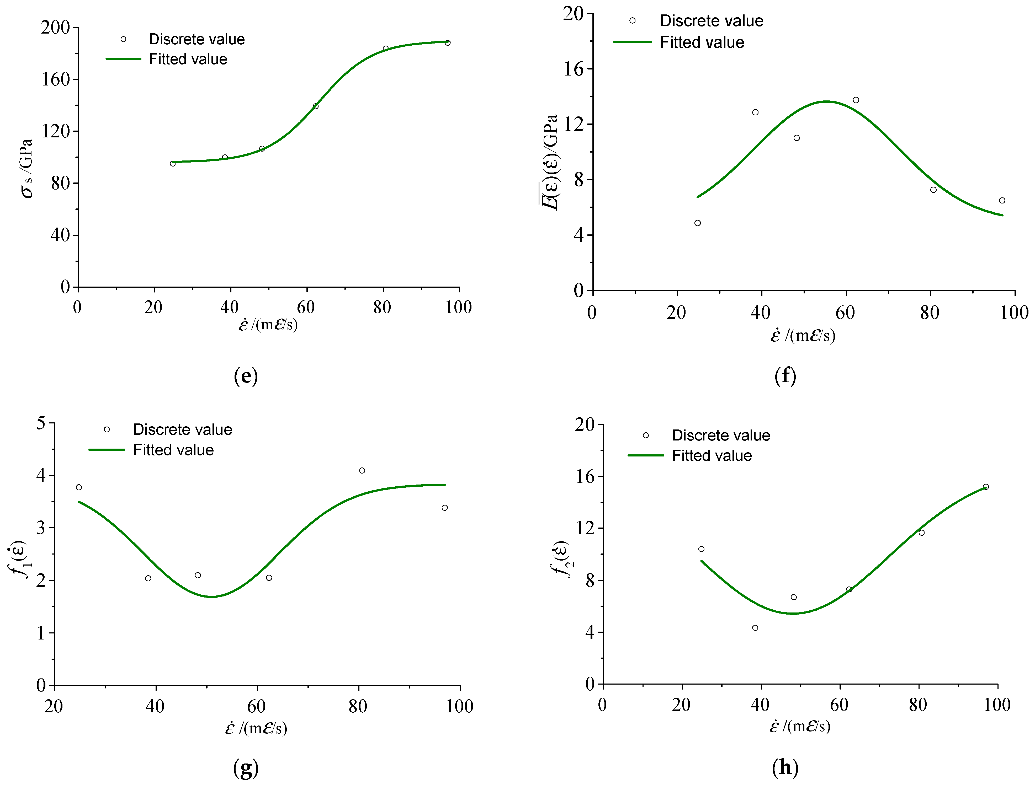
3.3.2. Parameter Analysis of the Coal Measures Rock B-G Damage Constitutive Model under Dynamic Load

The relationships between the fitting parameters $E$, $E_0$, $E_1$, ${\eta }_1$, ${\sigma }_{\mathrm{s}}$, $\overline{E(\epsilon )}$, $f_1$ as well as $f_2$ and the strain rate $E(\dot{\epsilon })$ are established. Thus, the expressions of $E(\dot{\epsilon })$, $E_0(\dot{\epsilon })$, $E_1(\dot{\epsilon })$, ${\eta }_1(\dot{\epsilon })$, ${\sigma }_{\mathrm{s}}(\dot{\epsilon })$, $\overline{E(\epsilon )}(\dot{\epsilon })$, $f_1(\dot{\epsilon })$ and $f_2(\dot{\epsilon })$ can be obtained, which are illustrated in Equations (78) to (85). Moreover, the fitting results are shown in Figure 18.

$$E(\dot{\epsilon })=14.03+\frac{675.45}{40.03\times \sqrt{\mathsf{\pi }/2}}{e}^{-2\times {(\frac{\dot{\epsilon }-77.72}{40.03})}^2},$$

(78)

$$E_0(\dot{\epsilon })=5.63+\frac{577.85}{6.20\times \sqrt{\mathsf{\pi }/2}}{e}^{-2\times {(\frac{\dot{\epsilon }-42.86}{6.20})}^2},$$

(79)

$$E_1(\dot{\epsilon })=3.87+\frac{504.54}{12.73\times \sqrt{\mathsf{\pi }/2}}{e}^{-2\times {(\frac{\dot{\epsilon }-67.43}{12.73})}^2},$$

(80)

$${\eta }_1(\dot{\epsilon })=-2.32+\frac{44.90}{20.82\times \sqrt{\mathsf{\pi }/2}}{e}^{-2\times {(\frac{\dot{\epsilon }-84.08}{20.82})}^2},$$

(81)

$${\sigma }_{\mathrm{s}}(\dot{\epsilon })=189.68+\frac{96.03-189.68}{1+e^{(\frac{\dot{\epsilon }-63.21}{7.01})}},$$

(82)

$$\overline{E(\epsilon )}(\dot{\epsilon })=4.96+\frac{373.06}{34.31\times \sqrt{\mathsf{\pi }/2}}{e}^{-2\times {(\frac{\dot{\epsilon }-55.33}{34.31})}^2},$$

(83)

$$f_1(\dot{\epsilon })=3.83+\frac{-72.40}{27.02\times \sqrt{\mathsf{\pi }/2}}{e}^{-2\times {(\frac{\dot{\epsilon }-50.91}{27.02})}^2},$$

(84)

$$f_2(\dot{\epsilon })=16.64+\frac{-686.28}{48.83\times \sqrt{\mathsf{\pi }/2}}{e}^{-2\times {(\frac{\dot{\epsilon }-47.97}{48.83})}^2}.$$

(85)

The expressions of $E(\dot{\epsilon })$, $E_0(\dot{\epsilon })$, $E_1(\dot{\epsilon })$, ${\eta }_1(\dot{\epsilon })$, $\overline{E(\epsilon )}(\dot{\epsilon })$, $f_1(\dot{\epsilon })$ and $f_2(\dot{\epsilon })$ can be uniformly expressed by Equation (86), which is

$$F(\dot{\epsilon })=y(0)+\frac{A}{w\sqrt{\mathsf{\pi }/2}}{e}^{-2\times {(\frac{\dot{\epsilon }-B}{w})}^2}=y(0)+\frac{A}{\frac{w}{2}\sqrt{2\mathsf{\pi }}}{e}^{-\frac{{(\dot{\epsilon }-B)}^2}{2{(\frac{w}{2})}^2}}.$$

(86)

where the expression of ${\sigma }_{\mathrm{s}}(\dot{\epsilon })$ can be expressed by the following equation:

$${\sigma }_{\mathrm{s}}(\dot{\epsilon })=A+\frac{B-A}{1+e^{\frac{\dot{\epsilon }-C}{D}}}.$$

(87)

According to Equation (86), the variation law that parameters $E$, $E_0$, $E_1$, ${\eta }_1$, ${\sigma }_{\mathrm{s}}$, $\overline{E(\epsilon )}$, $f_1$ and $f_2$ changing with the strain rate $\dot{\epsilon }$ obey the Gaussian distribution (normal distribution). Furthermore, the variation law that ${\sigma }_{\mathrm{s}}(\dot{\epsilon })$ changes with strain rate $\dot{\epsilon }$ obeys the Gaussian distribution and the Boltzmann distribution.

4. The Yield Rule and Fracture Criterion of Floor Coal Measures Surrounding Rock under the Coupled Static-Dynamic Load Disturbance

4.1. Yield Rule of Coal Measures Rock Damage under Dynamic Load Effect

Damage criterion is one of the essential contents of strength theory, which can illustrate the failure law of materials under complex stress effects [46]. At present, the strength theory can be divided into three categories. First is the simple shear strength theory, including the Treasca yield criterion, the Mohr-Coulomb yield criterion, etc. In addition, the twin shear strength theory includes the twin shear yield criterion and the generalized failure yield criterion. Moreover, the octahedron shear stress strength theory (tri-shear strength theory), including the Huber-von Mises yield criterion and Drucker-Prager (D-P) yield criterion, etc. These are all yield failure criteria corresponding to a certain material type and have been applied in their respective fields [47]. However, they all have corresponding shortcomings. For example, the Mohr-Coulomb criterion does not consider the influence of the intermediate principal stress ${\sigma }_2$, and the Drucker-Prager criterion cannot reflect the difference between the tensile meridian and the compressive meridian of the limit surface. Therefore, the unified strength theory came into being [48].

The expression of the twin shear unified strength theory is shown in Equation (88), which is expressed by some material parameters, such as cohesion force $c_0$, friction angle $\phi$, principal stress ${\sigma }_1$, ${\sigma }_2$ and ${\sigma }_3$.

$$\begin{array}{ll}{\sigma }_1-\frac{1-\sin \phi }{(1+b)(1+\sin \phi )}(b{\sigma }_2+{\sigma }_3)=\frac{2c_0\cos \phi }{1+\sin \phi }& {\sigma }_2\le \frac{1}{2}({\sigma }_1+{\sigma }_3)-\frac{\sin \phi }{2}({\sigma }_1-{\sigma }_3)\\ \frac{1}{1+b}({\sigma }_1+b{\sigma }_2)-\frac{1-\sin \phi }{1+\sin \phi }{\sigma }_3=\frac{2c_0\cos \phi }{1+\sin \phi }& {\sigma }_2\ge \frac{1}{2}({\sigma }_1+{\sigma }_3)-\frac{\sin \phi }{2}({\sigma }_1-{\sigma }_3)\end{array},$$

(88)

where b is the influence weight coefficient reflecting the intermediate principal stress, which can be expressed by the tensile ultimate strength ${\sigma }_{\mathrm{s}}$ and shear ultimate strength ${\tau }_{\mathrm{s}}$.

$$b=\frac{2{\tau }_s-{\sigma }_s}{{\sigma }_s-{\tau }_s}.$$

(89)

The rock yield criterion under dynamic load is the research focus of the rock material strength theory. It has the non-linearity characteristic, and the relevant parameters are the function of strain rate $\dot{\epsilon }$. This paper uses the unified strength theory to study the yield failure criterion of the floor surrounding rock under the coupled static-dynamic loading disturbance. It is considered that the cohesion force $c_0$ is a function of strain $\epsilon$ and strain rate $\dot{\epsilon }$, which is shown as follows:

$$c_0=c_0(\epsilon ,\dot{\epsilon }).$$

(90)

The Mohr-Coulomb yield criterion is a special case of the unified strength criterion, but the relevant parameters represent the inherent properties of rock. However, the parameters will not change with the criteria. Therefore, the Mohr-Coulomb yield criterion can be used to solve relevant parameters. The Mohr-Coulomb yield criterion expressed by principal stress is shown as Equation (91).

$${\sigma }_1-{\sigma }_3=({\sigma }_1+{\sigma }_3)\sin \phi +2C_0\cos \phi .$$

(91)

when it is uni-axial compression, ${\sigma }_1=0$, so

$$C_0=\frac{1+\sin \phi }{2\cos \phi }{\sigma }_3.$$

(92)

From the pre-peak B-G constitutive Equation (77) derived in this paper, Equation (93) is obtained as follows:

$${\sigma }_3=\frac{{\eta }_{1}E}{E_0(E+E_1)}\left\{\begin{array}{l}(E_0+E_1)\exp [-{(\frac{\epsilon }{f_2(\dot{\epsilon })})}^{f_1(\dot{\epsilon })}]\dot{\epsilon }\\ +\frac{E_0{E}_1}{{\eta }_1}\exp [-{(\frac{\epsilon }{f_2(\dot{\epsilon })})}^{f_1(\dot{\epsilon })}]\epsilon -\frac{E_0+E+E_1}{E}E(\epsilon )\dot{\epsilon }\end{array}\right\}.$$

(93)

Equation (93) is taken into Equation (92),

$$C_0(\epsilon ,\dot{\epsilon })=\frac{1+\sin \phi }{2\cos \phi }\frac{{\eta }_{1}E}{E_0(E+E_1)}\left\{\begin{array}{l}(E_0+E_1)\exp [-{(\frac{\epsilon }{f_2(\dot{\epsilon })})}^{f_1(\dot{\epsilon })}]\dot{\epsilon }\\ +\frac{E_0{E}_1}{{\eta }_1}\exp [-{(\frac{\epsilon }{f_2(\dot{\epsilon })})}^{f_1(\dot{\epsilon })}]\epsilon -\frac{E_0+E+E_1}{E}E(\epsilon )\dot{\epsilon }\end{array}\right\}.$$

(94)

Then, if Equation (94) is taken into Equation (88), the expression of the twin shear uniform strength theory considering the strain rate effect can be obtained.

$$\begin{array}{c}{\sigma }_1-\frac{1-\sin \phi }{(1+b)(1+\sin \phi )}\left(b{\sigma }_2+{\sigma }_3\right)=\frac{{\eta }_{1}E}{E_0\left(E+E_1\right)}\left\{\begin{array}{c}\left(E_0+E_1\right)\exp \left[-{\left(\frac{\epsilon }{f_2(\dot{\epsilon })}\right)}^{f_1(\overline{\epsilon })}\right]\dot{\epsilon }\hfill \\ +\frac{E_0{E}_1}{{\eta }_1}\exp \left[-{\left(\frac{\epsilon }{f_2(\dot{\epsilon })}\right)}^{f_1(\dot{\epsilon })}\right]\epsilon -\frac{E_0+E+E_1}{E}E(\epsilon )\dot{\epsilon }\hfill \end{array}\right\}{\sigma }_2\le \frac{1}{2}\left({\sigma }_1+{\sigma }_3\right)-\frac{\sin \phi }{2}\left({\sigma }_1-{\sigma }_3\right).\hfill \\ \frac{1}{1+b}\left({\sigma }_1+b{\sigma }_2\right)-\frac{1-\sin \phi }{1+\sin \phi }{\sigma }_3=\frac{{\eta }_{1}E}{E_0(E+E)}\left\{\begin{array}{c}\left(E_0+E_1\right)\exp \left[-{\left(\frac{\epsilon }{f_2(\dot{\epsilon })}\right)}^{f_1\dot{\epsilon }}\right]\dot{\epsilon }\hfill \\ +\frac{E_0{E}_1}{{\eta }_1}\exp \left[-{\left(\frac{\epsilon }{f_2(\dot{\epsilon })}\right)}^{f_1(\dot{\epsilon })}\right]\epsilon -\frac{E_0+E+E_1}{E}E(\epsilon )\dot{\epsilon }\hfill \end{array}\right\}{\sigma }_2\ge \frac{1}{2}\left({\sigma }_1+{\sigma }_3\right)-\frac{\sin \phi }{2}\left({\sigma }_1-{\sigma }_3\right).\hfill \end{array}$$

(95)

4.2. The Fracture Criterion of Floor Strata under the Coupled Static-Dynamic Loading Disturbance

According to material mechanics theories, the principal stress under the plane strain state is

$$\left.\begin{array}{c}{\sigma }_1\\ {\sigma }_3\end{array}\right\}=\frac{{\sigma }_x+{\sigma }_y}{2}\pm \sqrt{{\left(\frac{{\sigma }_x-{\sigma }_y}{2}\right)}^2+{\tau }_{xy}^2}.$$

(96)

Under the plane strain state, the principal stress vertical to the plane direction is

$${\sigma }_2=\mu ({\sigma }_1+{\sigma }_3).$$

(97)

where $\mu$ is the Poisson ratio.

Define $F_R=\left(\frac{1}{2}-\mu \right)\left({\sigma }_1+{\sigma }_3\right)-\frac{\sin \phi }{2}\left({\sigma }_1-{\sigma }_3\right)$. Also, define $F_D$ as

$$F_D=\left\{\begin{array}{c}{\sigma }_1-\frac{1-\sin \phi }{(1+b)(1+\sin \phi )}\left(b{\sigma }_2+{\sigma }_3\right)-\frac{{\eta }_{1}E}{E_0\left(E+E_1\right)}\left\{\begin{array}{c}\left(E_0+E_1\right)\exp \left[-{\left(\frac{\epsilon }{f_2(\dot{\epsilon })}\right)}^{f_1(\dot{\epsilon })}\right]\dot{\epsilon }\hfill \\ +\frac{E_0{E}_1}{{\eta }_1}\exp \left[-{\left(\frac{\epsilon }{f_2(\dot{\epsilon })}\right)}^{f_1(\dot{\epsilon })}\right]\epsilon -\frac{E_0+E+E_1}{E}E(\epsilon )\dot{\epsilon }\hfill \end{array}\right\}{F}_R\ge 0\hfill \\ \frac{1}{1+b}\left({\sigma }_1+b{\sigma }_2\right)-\frac{1-\sin \phi }{1+\sin \phi }{\sigma }_3-\frac{{\eta }_{1}E}{E_0\left(E+E_1\right)}\left\{\begin{array}{c}\left(E_0+E_1\right)\exp \left[-{\left(\frac{\epsilon }{f_2(\dot{\epsilon })}\right)}^{f_1(\dot{\epsilon })}\right]\dot{\epsilon }\hfill \\ +\frac{E_0{E}_1}{{\eta }_1}\exp \left[-{\left(\frac{\epsilon }{f_2(\dot{\epsilon })}\right)}^{f_1(\dot{\epsilon })}\right]\epsilon -\frac{E_0+E+E_1}{E}E(\epsilon )\dot{\epsilon }\hfill \end{array}\right\}{F}_R<0\hfill \end{array}\right.$$

(98)

Equations (96) and (97) are taken into $F_R$ and $F_D$ respectively,

$$F_R=\left(\frac{1}{2}-\mu \right)\left({\sigma }_x+{\sigma }_y\right)-\sin \phi \sqrt{{\left(\frac{{\sigma }_x-{\sigma }_y}{2}\right)}^2+{\tau }_{xy}^2},$$

(99)

$$F_D=\left\{\begin{array}{c}\left\{\begin{array}{c}\left\{\begin{array}{c}\left.\frac{1}{2}+\left(\frac{1}{2}+\mu b\right)\frac{1-\sin \phi }{(1+b)(1+\sin \phi )}\right]\left({\sigma }_x+{\sigma }_y\right)\hfill \\ +\frac{2+(1+\sin \phi )b}{(1+b)(1+\sin \phi )}\sqrt{{\left(\frac{{\sigma }_x-{\sigma }_y}{2}\right)}^2+{\tau }_{xy}^2}\hfill \end{array}\right\}-\frac{{\eta }_{1}E}{E_0\left(E+E_1\right)}\left\{\begin{array}{c}\left(E_0+E_1\right)\exp \left[-{\left(\frac{\epsilon }{f_2(\dot{\epsilon })}\right)}^{f_1(\dot{\epsilon })}\right]\dot{\epsilon }\hfill \\ +\frac{E_0{E}_1}{{\eta }_1}\exp \left[-{\left(\frac{\epsilon }{f_2(\dot{\epsilon })}\right)}^{f_1(\dot{\epsilon }}\right]\epsilon -\frac{E_0+E+E_1}{E}E(\epsilon )\dot{\epsilon }\hfill \end{array}\right\}{F}_R\ge 0\hfill \end{array}\right.\hfill \\ \left\{\begin{array}{c}\left\{\begin{array}{c}\left[\frac{1+2\mu b}{2(1+b)}-\frac{1-\sin \phi }{2(1+\sin \phi )}\right]\left({\sigma }_x+{\sigma }_y\right)\hfill \\ +\left(\frac{1}{1+b}+\frac{1-\sin \phi }{1+\sin \phi }\right)\sqrt{{\left(\frac{{\sigma }_x-{\sigma }_y}{2}\right)}^2+{\tau }_{xy}^2}\hfill \end{array}\right\}-\frac{{\eta }_{E}E}{E_0\left(E+E_1\right)}\left\{\begin{array}{c}\left(E_0+E_1\right)\exp \left[-{\left(\frac{\epsilon }{f_2(\dot{\epsilon })}\right)}^{f_1(\dot{\epsilon })}\right]\dot{\epsilon }\hfill \\ +\frac{E_0{E}_1}{{\eta }_1}\exp \left[-{\left(\frac{\epsilon }{f_2(\dot{\epsilon })}\right)}^{f_1(\dot{s}}\right]\epsilon -\frac{E_0+E+E_1}{E}E(\epsilon )\dot{\epsilon }\hfill \end{array}\right\}{F}_R<0\hfill \end{array}\right.\hfill \end{array}\right.$$

(100)

where the expressions of ${\sigma }_x$, ${\sigma }_y$, and ${\tau }_{xy}$ are Equations (23)–(25), respectively, when the floor rock strata in goaf are under the centralized dynamic load effect. Moreover, when the floor rock strata in goaf are under the uniform dynamic load effect, the expressions of ${\sigma }_x$, ${\sigma }_y$ and ${\tau }_{xy}$ are Equation (27), Equation (28) and Equation (29) respectively.

Considering the floor rock in goaf is brittle material, the fracture criterion of the floor rock in goaf under the coupled static-dynamic loading disturbance is

$$F_D\ge 0.$$

(101)

5. Conclusions

In this paper, the damage evolution and fracture mechanism of floor strata in goaf under the coupled static-dynamic loading disturbance are studied from the aspects of floor strata stress distribution state, rock damage evolution constitutive model, and rock fracture criterion under the coupled static-dynamic loading disturbance. The main conclusions are drawn as follows:

1.

Based on the systematic analysis of the floor stress distribution state, the mining dynamic load coefficients of the intermediate fracture collapse and overall collapse in the roof and the overlying strata are solved by the floor beam model. The response mechanism of the floor strata stress state under the action of concentrated and uniform dynamic loads is established. Also, the calculation formula for the stress distribution at any position in the complete floor strata is given under the coupled static-dynamic loading disturbance.

2.

Combining the advantages of the Bingham and Generalized-Boydin models, the coal measure rock constitutive model under dynamic load (B-G Model) is established. By including the damage evolution model, the coal measures rock constitutive model (B-G damage model) under dynamic load is presented. The nonlinear regression fitting method is used to solve the parameters by using the experimental data. The fitting results show that the new model can present the constitutive characteristics of coal measure rock under dynamic load. Also, the variation law of the model parameters changing with strain rate is analyzed, and the unified mathematical expression is given with the strain rates as parameters.

3.

On the basis of the twin-shear unified strength yield criterion and the B-G damage constitutive model, the twin-shear unified strength damage and fracture criterion of coal measure rocks under the disturbance of coupled static-dynamic loading is established. This criterion takes the rock damage and strain rate into account. At last, we use the stress distribution expression of any position in the floor strata under the centralized and uniform dynamic load to create a collapse criterion of the floor strata in goaf under the disturbance of coupled static-dynamic loading.

In this paper, only the parameters of the B-G damage constitutive model are solved to verify the pre-peak section, and only the fracture criterion of the floor strata under the coupled static-dynamic loading disturbance is proposed. Therefore, in future studies, the reliability of the B-G damage constitutive model of coal measure rock under the coupled static-dynamic loading disturbance will be further verified through mathematical solutions and numerical calculation methods. Moreover, regarding the fracture criterion, the influence of various factors on the damage and fracture process of floor strata could also be further analyzed.

References

1. National Development and Reform Commission; National Energy Administration. ‘14th Five-Year’ Modern Energy System. Planning. Available online: https://www.gov.cn/zhengce/zhengceku/2022-03/23/content_5680759.htm (accessed on 29 January 2024).
2. Energy Institute. Statistical Review of World Energy 2023. Available online: https://www.energyinst.org/statistical-review (accessed on 29 January 2024).
3. Xie, H.P.; Wu, L.X.; Zheng, D.Z. Prediction on the energy consumption and coal demand of China in 2025. J. China Coal Soc. 2019, 44, 1949–1960. [Google Scholar]
4. Jia, Z.J.; Wen, S.Y.; Sun, Z. Current relationship between coal consumption and the economic development and China’s future carbon mitigation policies. Energy Policy 2022, 162, 112812. [Google Scholar] [CrossRef]
5. Xie, H.P. Research review of the state key research development program of China: Deep rock mechanics and mining theory. J. China Coal Soc. 2019, 44, 1283–1305. [Google Scholar]
6. He, M.C.; Wang, Q.; Wu, Q.Y. Innovation and future of mining rock mechanics. J. Rock Mech. Geotech. 2021, 13, 1–21. [Google Scholar] [CrossRef]
7. Kang, H.P.; Gao, F.Q.; Xu, G.; Ren, H.W. Mechanical behaviors of coal measures and ground control technologies for China’s deep coal mines –A review. J. Rock Mech. Geotech. 2023, 15, 37–65. [Google Scholar] [CrossRef]
8. Wagner, H. Deep Mining: A Rock Engineering Challenge. Rock Mech. Rock Eng. 2019, 52, 1417–1446. [Google Scholar] [CrossRef]
9. Xie, H.; Gao, M.; Zhang, R.; Peng, G.; Wang, W.; Li, A. Study on the Mechanical Properties and Mechanical Response of Coal Mining at 1000 m or Deeper. Rock Mech. Rock Eng. 2019, 52, 1475–1490. [Google Scholar] [CrossRef]
10. Li, X.B.; Gong, F.Q.; Tao, M.; Dong, L.G.; Du, K.; Ma, C.D.; Zhou, Z.L.; Yin, T.B. Failure mechanism and coupled static-dynamic loading theory in deep hard rock mining: A review. J. Rock Mech. Geotech. 2017, 9, 767–782. [Google Scholar] [CrossRef]
11. Ranjith, P.G.; Zhao, J.; Ju, M.; De Silva, R.V.; Rathnaweera, T.D.; Bandara, A.K. Opportunities and Challenges in Deep Mining: A Brief Review. Engineering 2017, 3, 546–551. [Google Scholar] [CrossRef]
12. Charles, F. Some challenges of deep mining. Engineering 2017, 3, 527–537. [Google Scholar]
13. Yang, S.Q.; Chen, M.; Jing, H.W.; Chen, K.F.; Meng, B. A case study on large deformation failure mechanism of deep soft rock roadway in Xin’An coal mine, China. Eng. Geol. 2016, 217, 89–101. [Google Scholar] [CrossRef]
14. Zhang, J.J.; Xu, K.L.; Reniers, G.; You, G. Statistical analysis the characteristics of extraordinarily severe coal mine accidents (ESCMAs) in China from 1950 to 2018. Process Saf. Environ. Prot. 2020, 133, 332–340. [Google Scholar] [CrossRef]
15. Bai, H.B.; Miao, X.X. Hydrogeological characteristics and mine water inrush prevention of late Paleozoic coalfields. J. China Univ. Min. Technol. 2016, 45, 1–10. [Google Scholar]
16. Zhang, C.; Bai, Q.; Han, P. A review of water rock interaction in underground coal mining: Problems and analysis. Bull. Eng. Geol. Environ. 2023, 82, 157. [Google Scholar] [CrossRef]
17. Miao, X.X.; Bai, H.B. Water-resisting characteristics and distribution rule of carbonate strata in the top of Ordovician in North China. J. China Coal Soc. 2011, 36, 185–193. [Google Scholar]
18. Gui, H.R.; Song, X.M.; Lin, M.L. Water-inrush mechanism research mining above karst confined aquifer and applications in North China coalmines. Arabian J. Geosci. 2017, 10, 180. [Google Scholar] [CrossRef]
19. Sun, W.; Zhou, W.; Jiao, J. Hydrogeological classification and water inrush accidents in China’s coal mines. Mine Water Environ. 2016, 35, 214–220. [Google Scholar] [CrossRef]
20. Liu, Y.; Dai, F.; Pei, P.D. A wing-crack extension model for tensile response of saturated rocks under coupled static-dynamic loading. Int. J. Rock Mech. Min. 2021, 146, 104893. [Google Scholar] [CrossRef]
21. Ma, D.; Duan, H.Y.; Li, X.B.; Li, Z.H.; Zhou, Z.L.; Li, T.B. Effects of seepage-induced erosion on nonlinear hydraulic properties of broken red sandstones. Tunn. Undergr. Space Tech. 2019, 91, 102993. [Google Scholar] [CrossRef]
22. Ma, D.; Duan, H.Y.; Zhang, J.X. Solid grain migration on hydraulic properties of fault rocks in underground mining tunnel: Radial seepage experiments and verification of permeability prediction. Tunn. Undergr. Space Tech. 2022, 126, 104525. [Google Scholar] [CrossRef]
23. Shi, L.; Qiu, M.; Wang, Y.; Qu, X.; Liu, T. Evaluation of water inrush from underlying aquifers by using a modified water-inrush coefficient model and water-inrush index model: A case study in Feicheng coalfield, China. Hydrogeol. J. 2019, 27, 2105–2119. [Google Scholar] [CrossRef]
24. Li, H.; Bai, H.; Ma, D.; Xu, J. Experimental study on mining-induced failure depth lagging coal wall secondary deepening rule. J. Min. Saf. Eng. 2016, 33, 318–323. [Google Scholar]
25. Li, H.L.; Bai, H.B.; Ma, D. Physical simulation testing research on mining dynamic loading effect and induced coal seam floor failure. J. Min. Saf. Eng. 2018, 35, 366–372. [Google Scholar]
26. Li, H.L.; Bai, H.B. Simulation research on the mechanism of water inrush from fractured floor under the dynamic load induced by roof caving: Taking the Xinji Second Coal Mine as an example. Arabian J. Geosci. 2019, 12, 1–24. [Google Scholar] [CrossRef]
27. Zhou, Z.H.; Cao, P.; Ye, Z.Y. Crack propagation mechanism of compression-shear rock under static-dynamic loading and seepage water pressure. J. Cent. South Univ. 2014, 21, 1565–1570. [Google Scholar] [CrossRef]
28. Gai, Q.K.; Gao, Y.B.; Huang, L.; Shen, X.Y.; Li, Y.B. Microseismic response difference and failure analysis of roof and floor strata under dynamic load impact. Eng. Failure Anal. 2023, 143 Pt A, 106874. [Google Scholar] [CrossRef]
29. Shao, J.; Zhang, Q.; Zhang, W. Evolution of mining-induced water inrush disaster from a hidden fault in coal seam floor based on a coupled stress–seepage–damage model. Geomech. Geophys. Geo-Energy Geo-Resour. 2024, 10, 78. [Google Scholar] [CrossRef]
30. Xie, H.P.; Lu, J.; Li, C.B.; Li, M.H.; Gao, M.Z. Experimental study on the mechanical and failure behaviors of deep rock subjected to true triaxial stress: A review. Int. J. Min. Sci. Technol. 2022, 32, 915–950. [Google Scholar] [CrossRef]
31. He, M.C.; Wang, Q. Rock dynamics in deep mining. Int. J. Min. Sci. 2023, 33, 1065–1082. [Google Scholar]
32. Wen, Z.; Meng, F.; Jiang, Y.; Jing, S. Development and application of a series of experimental devices for coal mining dynamic behavior research. Geomech. Geophys. Geo-Energy Geo-Resour. 2022, 8, 71. [Google Scholar] [CrossRef]
33. Xie, J.; Ning, S.; Zhu, W.; Wang, X.; Hou, T. Influence of Key Strata on the Evolution Law of Mining-Induced Stress in the Working Face under Deep and Large-Scale Mining. Minerals 2023, 13, 983. [Google Scholar] [CrossRef]
34. Qian, M.G.; Shi, P.W.; Xu, J.L. Mine Pressure and Rock Layer Control; China University of Mining and Technology Press: Xuzhou, China, 2011. [Google Scholar]
35. Dong, Z.X.; Shan, R.L. Study on Constitutive Properties of Rocks under High Strain Rates. Eng. Blasting 1999, 6, 5–9. [Google Scholar]
36. Yang, R.; Bawden, W.F.; Katsabanis, P.D. New constitutive model for blast damage. Int. J. Rock. Mech. Min. Sci. Geomech. Abstr. 1996, 33, 245–254. [Google Scholar] [CrossRef]
37. Gao, W.X.; Yang, J.; Jin, Q.K. Study on Dynamic Damage Model of Rock. Eng. Blasting 1999, 5, 5–9. [Google Scholar]
38. Li, M. Research on Rupture Mechanisms of Coal Measures Sandstone under High Temperature and Impact Load. Ph.D. Dissertation, China University of Mining & Technology, Xuzhou, China, 2014. [Google Scholar]
39. Li, M.; Mao, X.B.; Cao, L.L. Experimental study of mechanical properties on strain rate effect of sandstones after high temperature. Rock Soil Mech. 2014, 35, 3479–3488. [Google Scholar]
40. Li, J.G. The Application of the Constitutive Damage Model of Rock and Soil in Problems of Impact Dynamics. Ph.D. Dissertation, University of Science and Technology of China, Hefei, China, 2007. [Google Scholar]
41. Lemaitre, J. A continuous damage mechanics model for ductile fracture. J. Eng. Mater. Technol. 1985, 107, 83–89. [Google Scholar] [CrossRef]
42. Xie, L.X.; Zhao, G.M.; Meng, X.R. Research on Excess Stress Constitutive Model of Rock under Impact Load. Chin. J. Rock Mech. Eng. 2013, 32, 2772–2781. [Google Scholar]
43. Kinoshita, S.; Sato, K.; Kawakita, M. On the mechanical behavior of rocks under impulsive loading. Bull. Fac. Eng. Hokkaido Univ. 1977, 8, 51–62. [Google Scholar]
44. Yu, Y.L. Rock Dynamics; University of Science and Technology Beijing Press: Beijing, China, 1990. [Google Scholar]
45. Zheng, Y.L.; Xia, S.Y. Viscoelastic Damage Constitutive Model for Rock. Chin. J. Rock Mech. Eng. 1996, 15, 428–432. [Google Scholar]
46. Yu, M.H. Advances in Strength Theories for Materials under Complex Stress State in the 20th Century. Adv. Mech. 2004, 34, 529–560. [Google Scholar] [CrossRef]
47. Yu, M.H. Linear and Nonlinear Unified Strength Theory. Chin. J. Rock Mech. Eng. 2007, 26, 662–669. [Google Scholar]
48. Yu, M.H. Unified Strength Theory for Geomaterials and its Applications. Chin. J. Geotech. Eng. 1994, 16, 1–10. [Google Scholar]
Figure 1. The support pressure distribution of floor strata.
Processes 12 01513 g001
Figure 2. Floor support stress distribution law (X-X section plane).
Processes 12 01513 g002
Figure 3. Floor support pressure distribution law (Y-Y section plane).
Processes 12 01513 g003
Figure 4. The normal force on the boundary of a half-plane body.
Processes 12 01513 g004
Figure 5. The half-plane body under the action of the distributed force on the boundary.
Processes 12 01513 g005
Figure 6. Simplified distribution of the floor support pressure (X-X axis section).
Processes 12 01513 g006
Figure 7. Simplified distribution of the floor support pressure (Y-Y axis section).
Processes 12 01513 g007
Figure 8. Collapse forms of roof strata (Y-Y axis section). (a) Broken collapse; (b) Overall collapse.
Processes 12 01513 g008
Figure 9. Impact mechanics model of a floor rock beam. (a) Concentrated dynamic load; (b) Uniform dynamic load.
Processes 12 01513 g009
Figure 10. The simplified distribution of floor support force under concentrated dynamic load (Y-Y axis section).
Processes 12 01513 g010
Figure 11. The simplified distribution of floor support force under uniform dynamic load (Y-Y axis section).
Processes 12 01513 g011
Figure 12. Bingham constitutive model.
Processes 12 01513 g012
Figure 13. Generalized-Boydin constitutive model.
Processes 12 01513 g013
Figure 14. B-G constitutive model of rock under dynamic load effect.
Processes 12 01513 g014
Figure 15. Simplified B-G constitutive model.
Processes 12 01513 g015
Figure 16. The stress-strain curve of coal measures rock under different strain rates.
Processes 12 01513 g016
Figure 17. Comparison of experimental values and theoretical values of pre-peak stress-strain curves of coal measure sandstone under different strain rates. (a) Comparison of experimental values and theoretical values of pre-peak stress-strain curves of coal measures sandstone when ε ˙ = 24.79 ; (b) Comparison of experimental values and theoretical values of pre-peak stress-strain curves of coal measures sandstone when ε ˙ = 38 . 46 ; (c) Comparison of experimental values and theoretical values of pre-peak stress-strain curves of coal measures sandstone when ε ˙ = 48 . 25 ; (d) Comparison of experimental values and theoretical values of pre-peak stress-strain curves of coal measures sandstone when ε ˙ = 62 . 30 ; (e) Comparison of experimental values and theoretical values of pre-peak stress-strain curves of coal measures sandstone when ε ˙ = 80 . 65 ; (f) Comparison of experimental values and theoretical values of pre-peak stress-strain curves of coal measures sandstone when ε ˙ = 96 . 95 .
Processes 12 01513 g017aProcesses 12 01513 g017b
Figure 18. The variation law and the fitting curve of different parameters change with strain rate. (a) The fitting curve of E ( ε ˙ ) and strain rate; (b) The fitting curve of E 0 ( ε ˙ ) and strain rate; (c) The fitting curve of E 1 ( ε ˙ ) and strain rate; (d) The fitting curve of η 1 ( ε ˙ ) and strain rate; (e) The fitting curve of σ s ( ε ˙ ) and strain rate; (f) The fitting curve of E ( ε ) ¯ ( ε ˙ ) and strain rate; (g) The fitting curve of f 1 ( ε ˙ ) and strain rate; (h) The fitting curve of f 2 ( ε ˙ ) and strain rate.
Processes 12 01513 g018aProcesses 12 01513 g018b