Automatic Detection of Track and Fields in China from High-Resolution Satellite Images Using Multi-Scale-Fused Single Shot MultiBox Detector

Abstract

Object detection is facing various challenges as an important aspect in the field of remote sensing—especially in large scenes due to the increase of satellite image resolution and the complexity of land covers. Because of the diversity of the appearance of track and fields, the complexity of the background and the variety between satellite images, even superior deep learning methods have difficulty extracting accurate characteristics of track and field from large complex scenes, such as the whole of China. Taking track and field as a study case, we propose a stable and accurate method for target detection. Firstly, we add the “deconvolution” and “concat” module to the structure of the original Single Shot MultiBox Detector (SSD), where Visual Geometry Group 16 (VGG16) is served as a basic network, followed by multiple convolution layers. The two modules are used to sample the high-level feature map and connect it with the low-level feature map to form a new network structure multi-scale-fused SSD (abbreviated as MSF_SSD). MSF-SSD can enrich the semantic information of the low-level feature, which is especially effective for small targets in large scenes. In addition, a large number of track and fields are collected as samples for the whole China and a series of parameters are designed to optimize the MSF_SSD network through the deep analysis of sample characteristics. Finally, by using MSF_SSD network, we achieve the rapid and automatic detection of meter-level track and fields in the country for the first time. The proposed MSF_SSD model achieves 97.9% mean average precision (mAP) on validation set which is superior to the 88.4% mAP of the original SSD. Apart from this, the model can achieve an accuracy of 94.3% while keeping the recall rate in a high level (98.8%) in the nationally distributed test set, outperforming the original SSD method.

1. Introduction

Remote-sensing information extraction has encountered unprecedented opportunities and challenges. The rapid development of remote sensing technology has produced a large amount of multi-source heterogeneous data, which not only puts forward higher requirements for computing power, but also puts forward new requirements for data processing methods.

Target detection is an important topic associated with remote sensing information extraction. Experts and scholars have proposed many detection methods, from the earliest target matching method based on template matching, the method based on prior knowledge to the target detection method based on object image analysis [1]. These methods have achieved remarkable results in the detection of specific objects in remote sensing images, for example, road detection [2,3,4], vehicle detection [5,6,7], building testing [8,9,10], etc. However, the traditional target detection method cannot meet the accuracy and efficiency of remote sensing big data processing [11] and has the following problems and deficiencies:

(1)

The adopted region selection algorithm generates a large number of recommended regions, which are very redundant and cause a large time overhead;

(2)

Feature selection method is easy to be dominated by artificial features. Although good results had been achieved in specific target detection tasks, these features may be limited when encountering complex targets or scenarios.

(3)

Manual participation makes the extraction of target features no longer flexible and cannot realize automatic detection. Therefore, in order to meet the growing needs of users, intelligent target detection methods have emerged, as the time require.

Since the 1990s, machine learning methods, such as support vector machine [12], CRF [13], K-NN [14], boosting [15] and random Forest [16], can be applied to a small area by automatically constructing information extraction models based on a small number of sample data set through training and learning [17,18,19,20], and become the mainstream algorithms for remote sensing target detection. However, such algorithms have limited model parameter capacity and weak model generalization ability due to its construction based on merely a small amount of sample data.

In 2006, deep learning emerged [21]. Its powerful feature learning and expression ability makes it widely used in the field of computer vision. Different from the artificial design features, deep learning automatically learns the features from original data by means of a deep neural network structure, and its features are richer and more complex than the shallow features of former machine learning method. It can perfectly describe most features of a target and achieve accurate target detection. As an efficient learning framework for automatic extraction of target features, the convolutional neural network (CNN) [22] in deep learning methods has been widely used in object detection. In recent years, with the continuous improvements on its network models, breakthrough progress has been made in target detection, and the accuracy in multiple tasks has exceeded that of manual identification. These algorithms comprise Region-CNN (R-CNN) [23], Spatial Pyramid Pooling Convolutional Networks (SPP-Net) [24], Fast R-CNN [25], Faster R-CNN [26], You Only Look Once (YOLO) [27], SSD [28], etc. R-CNN is the first application of CNN in the field of target detection, and replaces the sliding window with manual design features, which was used in traditional target detection. R-CNN made a great breakthrough in target detection and now opens the upsurge of target detection based on deep learning. Unfortunately, R-CNN is trained in multiple stages which makes it cumbersome and time-consuming. The following SPP-Net, Fast R-CNN and Faster R-CNN are improvements to R-CNN and could improve the speed and accuracy of CNN. However, they are all target detection algorithms based on candidate regions. Due to these methods need to generate pre-selected windows through sliding windows, the calculation is relatively large and the real-time target detection cannot be achieved. In contrast, YOLO series and SSD algorithms are target detection algorithms based on regression methods, which use the idea of regression to determine target borders and categories in images, and greatly improve target detection speed. Among them, SSD combines the regression idea in YOLO and anchor mechanism in Faster R-CNN and uses multi-scale regional features of all positions in the whole map to perform regression, which not only maintains the fast speed of YOLO, but also ensures the accuracy of window prediction. Thus, we chose SSD to conduct research for this paper.

The great success of deep learning in the field of computer vision provides an important opportunity for intelligent extraction of large-data remote sensing information [29,30,31,32]. In recent years, many scholars have tried to introduce the neural network from Red-Green-Blue (RGB) three-band true color natural images into the field of remote sensing images. The results showed that deep learning-based methods is far better than traditional algorithm in target detection [33,34,35]. Even so, unlike ordinary images acquired on the ground using a camera at a horizontal viewing angle, remote sensing images are acquired from top to bottom in air or space, which results in remote sensing images viewed by large scales, large differences in illumination shadows, and the context of complex scene [36]. There are still obvious deficiencies in image understanding and feature extraction for current network model. Aiming at the detection object (track and field) in this paper, the excellent target detection network SSD, which takes into account the precision and speed, cannot achieve satisfactory results in track and field detection. Based on the framework of target detection network SSD, we proposed a multi-scale fusion network named as multi-scale-fused SSD (MSF_SSD), which could improve the detection accuracy of track and field in a wide range of areas, such as the whole of China.

The main contributions of our work are summarized in the following three points:

(1)

We make a sample library of more than 50,000 track and fields on a national basis (9.6 million square kilometers) for the first time through repeated testing and evaluation.

(2)

We add a deconvolution module and connection module to the SSD network model and redesign the parameters of the network. The new network model MSF_SSD improves the detection accuracy.

(3)

We realize the rapid detection of meter-level track and field nationwide for the first time, which achieved an accuracy of 94.3% while keep the recall rate in a high level (98.8%).

The reminder of this paper is organized as follows. Section 2 presents the materials and methodology of this paper. Section 3 introduces the experimental results and discussions. Section 4 gives the conclusions of this paper.

2. Materials and Methodology

By migrating the target detection model designed for natural images with RGB three-band in the field of computer vision and combining it with the characteristics of remote sensing images, it can achieve better results than those by traditional algorithms. However, it is still not ideal for real remote sensing applications, such as the detection of track and fields. Part of the reason is the lack of remote sensing sample libraries, and the target features and background are more complex in large-scale remote sensing scenarios than those in natural images.

It is very difficult to detect targets in a large remote sensing scene, compared with the natural images, the high complexity of the target and natural background scenes in remote sensing images of China and the huge differences in remote sensing images themselves make the semantic information of targets more complex and non-identity. The track and field features in the remote sensing images are very diverse, which results in the seemingly simple extraction becomes extremely complex. Not only the characteristics of track and field are very different themselves, but also many false targets are easy to be extracted inappropriately. For example, ponds with a circle of paths, highway overpasses, flowerbeds with paths, etc. all have partial or entire characteristics of track and field. In addition, the track and field across the country is a typical small target in a large-scale remote sensing image, which requires not only a large enough feature map to provide fine features and precise locations, but also sufficient semantic information to distinguish it from the background. Finally, in the face of remotely sensed big data, in order to realize track and field detection in China, the detection accuracy and recall rate must be guaranteed.

Aiming at solving the problems described above, the proposed method consists of three steps in this study: (1) Preprocess the remote sensing images and make the samples of track and field; (2) Design a MSF_SSD and train it based on the track and field samples. The well trained model is then used for detection; (3) Automatically detect the track and fields throughout China. The detailed workflow overview is presented in Figure 1.

2.1. Sample Preparation

Most of research works on image classification, location and detection are based on sub-datasets. There are many standard datasets in computer field, such as ImageNet [37], with more than 14 million images covering more than 20,000 categories. There are more than one million images have been clearly labeled category labels and object position labels in the images, which is a dataset that has been widely used in the field of deep learning research at present. Because of the particularity of remote sensing images, the difficulty in interpreting remote sensing features and the variety of remote sensing application scenarios, there are few data sets for in-depth learning training in remote sensing field. The target detection algorithm based on deep learning is essentially a supervised learning method, which should acquire the essential features of targets through a large amount of sample data, to predict and discriminate the unknown data accordingly.

In order to obtain training samples of track and field on standard high-resolution remote sensing images, the target characteristics must be analyzed first. Track and field samples are widely distributed with different characteristics. As Figure 2 shows, the common plastic track and fields usually appear in urban areas. Although the runway materials are plastic, the contents of its central area vary greatly, including cement fields, basketball courts, badminton courts, football fields, lawns and so on, and its size, aspect ratio are also different and may even be deformed. There are lots of track and fields made of muck, loess and cement in the rural and urban-rural areas. They are not only complex and diverse in materials, but also more random and irregular in size, shape and central area than those in city sports fields. Interchanges, freeway ramps and country trails have similar shapes to track and field and often contain vegetation in the middle. These features are very similar to track and field, but the cost of manual interpretation is too high. In order to produce effective training samples for track and field target detection, we establish a set of interpretation standards and production procedures for track and field sample library. We initially used semiautomatic marking software to efficiently increase the number of track and field images and form track and field samples with good quality and quantity such as training sets, validation sets and test sets. When selecting samples, we should consider the target feature definition, the number of negative samples, the network bearing capacity and so on. Based on the above considerations, the data we prepare for samples is images of Gaofen-2 (GF-2) satellite. GF-2 satellite was successfully launched on 19 August 2014, it was first turned on and imaged on 21 August 2014. GF-2 is one of the highest spatial resolution civilian land observation satellite in China, its spatial resolution is 0.8 m in panchromatic images and 3.2 m in multi-spectral images.

In this paper, the pixel factory software is used for pre-processing GF-2 images. Firstly, adaptive segmented linear stretching is performed on panchromatic images and multi-spectral images to enhance the sharpness and contrast of the original GF-2 images. Then we use the rational polynomial coefficients model to improve the positioning accuracy of images. Finally, we use the panchromatic fusion method to fuse the panchromatic images and multi-spectral images to generate the images with a spatial resolution of 1 m and three bands of RGB. The pre-processed GF-2 images’ size is too large to directly train, so the images need to be cropped before producing samples. The size of the samples is considered from two aspects: batch size and the number of negative samples. On one hand, the batch size determines the number of samples per input to the neural network, small batch size increases the randomness of the direction of the gradient, and this will make the network difficult to converge. Big batch size cannot only enhance the accuracy of the gradient descent direction, but also improve the efficiency of computer memory utilization, thereby reducing the number of iterations required to run a complete data set and speeding up the training of the model. However, due to the memory limitations of the GPU, in order to ensure as large batch size as possible, the size of the input image should not be too large. On the other hand, we must keep the number of negative samples to enhance the resistance to confusing features, so the size of the input image should not be too small. As our GPU is Titan XP, its memory is 12G, so we set the crop size to be 768 × 768, while the maximum batch size can be set to be 8 and the negative samples are enough. The process of cropping GF-2 images is shown in Figure 3.

After cropping the GF-2 image, we start to make the track and field samples. Different from the normal images, the diversity of the appearance of track and fields, the complexity of the background and the variety between GF-2 images make it more difficult to be detected. For example, the illumination and orientation can have different effects on images. In order to reduce the sensitivity to illumination, we write a function to randomly adjust the brightness of the image so that the data samples will randomly be distributed throughout the entire brightness range, which can improve the adaptability of data to brightness. The orientation of the camera may also interfere with the features of track and fields, except the rotation, the tall buildings or trees around the track and fields may cause shadows or occlusion. Firstly, we add a rotation enhancement to reduce the impact of rotation, then in order to solve the problem of shadows, we deliberately choose some track and fields with shadows when making samples. To solve the problem of occlusion, we use randomly cropping method to enhance the generalization ability of samples. The above three methods can effectively solve the problems caused by the orientation of the camera.

Besides, we establish a set of standards to label samples, in which the track and field samples cannot be limited to local areas and their types, shapes, colors and size need to be various. The purpose of this is to increase the applicability and generalization of the track and field samples to prevent over-fitting of the network. After many iterations of labeling, training, prediction, screening and correction, our track and field samples contain 10,000 training samples, 2000 validation samples and 44,000 test samples (including 4000 positive cases and 40,000 negative cases), of which the negative case picture is shown in Figure 4 and the sample point distribution is shown in Figure 5.

2.2. The Proposed Method

2.2.1. SSD

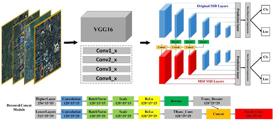
The paper uses VGG16 [38] as the basic network of SSD to extract low-level features of a target through a series of network layers conv1_x, conv2_x, conv3_x, and conv4_x. As shown in Figure 6, VGG16 are mainly composed of convolutional layers, relu layers, and pool layers. For example, conv1_x is organized by several network layers, such as “conv1_1-relu1_1-conv1_2-relu1_2-pool1”. Convolution layer is used to abstract the characteristics of a target, with kernel size is set to be 3, stride is set to be 1, pad is set to be 1, to maintain the image resolution of a feature graph after convolution. Relu layer is used to reduce the interdependence of network parameters and alleviate the problem of over-fitting. The Pool layer is used to reduce the latitude of a feature map and the amount of data. The pool method used in this research is Max Pooling, where kernel size is set to be 2, stride is set to be 2 and pad is set to be 0. With the deepening of the network, the resolution of feature images generated by each network layer gradually decreased (768, 384, or 192) and the number of feature images gradually increased (64, 128, or 256) till conv4_3 layer. At this time, VGG16 completes the task of extracting target features, and extracts 512 feature maps with a resolution of 96×96. MSF_SSD takes CON V4_3 as the first convolution layer to predict target confidence and position, and then adds multi-scale convolution layer.

There are three reasons to extract target features by using VGG16 pre-training model. The first one is that VGG16 replaces a larger convolution nucleus (11 × 11, 5 × 5) with several consecutive 3 × 3 convolution cores. For a given receptive field, it is better to use small convolution kernels than to use large convolution kernels. It is because that multiple nonlinear layers can increase the depth of the network to ensure learning more complex patterns. Secondly, the number of VGG16 network parameters is small, which can effectively reduce the detection time. Finally, the VGG16 pre-training model does not require a random initial value to train network, thus can increase the accuracy of the model and save the training time.

The original SSD method is based on VGG16 network, which generates a series of fixed-size bounding boxes and scores when detecting the presence of a target and obtains final detection results by using a non-maximum suppression algorithm. Each added convolution feature layer can generate predicted values through a set of convolution filters, including the confidence of the target category and the offset of the target relative to the default bounding boxes coordinates. In addition, SSD assigns a set of default bounding boxes to feature maps with different sizes, which are tiled on the feature map in a convolutional manner and then centered on the midpoint of each pixel on the feature map (offset = 0.5) to generate a number of columns of concentric default bounding boxes. The original SSD assigns different aspect ratios represented by ${\alpha }_r\in \left\{1,2,3,1/2,1/3\right\}$ to default boxes. By combining default boxes with different aspect ratios in multiscale feature maps, we will have a goal of various prediction results at different scales. We predict shape with respect to the default boxes positional deviation, and the target confidence level adhere to this category.

The added original convolutional layer SSD has a total of 6 convolutional layers, “conv4_3-conv5_2-conv6_2-conv7_2-conv8_2-conv9_2”, whose resolution is successively reduced, as indicated in blue in the Figure 7. The prediction layer behind the convolutional layer detects targets at different scales. The non-maximum suppression algorithm behind the prediction layer is the screening of detection frames.

2.2.2. The Proposed MSF_SSD Method

By analyzing the characteristics of track and fields in high resolution remote sensing images in Section 2.1, we can know that the variety of track and fields across China make the seemingly simple extraction extremely difficult. The semantic information of track and fields in remote sensing images is more complicated and not identical, and the nationwide track and field is a typical small target in remote sensing images. The original SSD uses different convolutional layers to predict targets of different sizes, and the lower layers are used to predict small targets, these layers’ feature maps have high resolution but their semantic information is not enough. The high-level layers are used to predict large targets, their semantic information is rich but the feature maps become small after many pooling. To detect the small targets, we need a large enough feature map to provide fine features and precise location, while also requiring enough semantic information to distinguish it from the background.

In order to solve the above problems, increase the accuracy rate and recall rate of the network, we propose a Multi-Scale-Fused SSD network based on the framework of the original SSD. MSF_SSD uses VGG-16 as the backbone network to generate low-level feature maps. On this basis, it expands the convolutional layers of multiple scales, then samples the high-level features through the “deconvolution” module and uses the “concat” module to fuse the high and the low layers’ features to enhance the semantics of the lower layers. The structure of the proposed MSF_SSD method is substantially similar to the original SSD, except that the first three convolution layers of MSF_SSD are displayed in red. Among them, the red conv4 _ 3 convolution layer is formed by the fusion of “conv7 _ 2, conv 6 _ 2, conv _ fc7 and conv4 _ 3” convolution layers. By analogy, the red conv_fc7 convolution layer is formed by the fusion of “conv 7_2, conv 6_2 and conv _fc7”, and the red conv 6_2 convolution layer is formed by the fusion of “conv 7_2 and conv 6_2”. The fusion process is divided into two steps: the first step is to change the high-level low-resolution feature map to the same size as its neighboring low-level feature map by “deconvolution” module, as shown in Figure 7. First, a convolutional layer conv_trans is added after each convolutional layer to change the number of feature maps in preparation for subsequent connection operations; Then, a batch normalization layer is added after conv_trans, and the distribution of the input value of any neuron in each layer of neural network is forcibly pulled back to the standard normal distribution with a mean value of 0 and the variance of 1 by the way of normalization, so that the active input value falls into non-linearity to make the gradient larger and make the learning convergence speed faster, and the training speed is greatly accelerated. Finally, a deconvolution layer is added behind the batch normalization layer, and we use the “concat” module to combine the sampled feature map with the adjacent low-level feature map.

In the experiment of this paper, we select the first four layers of the network as a fusion layer. The number and resolution of feature maps of “conv7_2, conv6_2, conv_fc7, conv4_3” and other layers are shown in

Table 1. MSF_SSD Network Top Four Feature Layers.

	conv4_3	conv_fc7	conv6_2	conv7_2
resolution	96	58	29	15
dimension	512	1024	512	256
trans_dimension	128	128	128	128
deconv_dimension	128	128	128	128
concat_dimension	512	384	256	128

. The deconvolution layer changes the number of feature maps per layer to 128. After using the “concat” module, the output of conv4_3 is 512, the output of conv_fc7 is 384, the output of conv6_2 is 256, and the output of conv7_2 is 128, which enhance the semantic information of the feature map at the scale. Previous work has proved [39] that convolutional neural network has been successfully used to increase target detection accuracy by acquiring semantic information for the detector’s lower layers. Here we only work out the fusion processing for the first four layers. There are two main considerations. On the one hand, the deconvolution layer and the adjacent are computational inefficient, so fusing the appropriate convolution layers can decrease computational costs. On the other hand, for the detection target of this paper, first of all, the track and field in high-resolution remote sensing image is small, and the small target is easier to be detected in the first few layers of MSF_SSD. Secondly, the background information of track and field is cumbersome, but the experience used in the network is insufficient. The MSF_SSD fusion means enrich the semantic information of the first few layers and can accurately complete the detection of track and field. Therefore, the fusion method of MSF_SSD in this paper can not only ensure the detection accuracy, but also can save on computational costs, which is of great significance in the application of target detection in large remote sensing scenes.

2.2.3. Network Training

Our network is trained in Caffe framework and the hardware environment is Titan XP GPU, CUDA 2.0 and Intel Xeon E5. Our experiments are all based on the pretrained network VGG16 base on ILSVRC CLS-LOC datasets. First, we set the appropriate network hyper parameters shown in

Table 2. Hyper parameters of MSF_SSD.

Hyper Parameters	Value
batch size	8
batch_lr	0.0001
max_iter	120,000
gamma	0.1
momentum	0.9
weight_decay	0.0005
learning rate	0.0001(iter < 50,000)
	0.00001 (80,000 < iter < 100,000)
	0.000001(100,000 < iter)

by a series of experiments. We use 10,000 training sets and 2000 validation sets to train the model, where size is set to be 768 × 768. We train the model by using the optimizer SGD with 0.9 momentum, 0.0005 weight decay, and batch size 8, and the maximum number of iterations is set to be 120 K. The initial learning rate at the beginning of training is set to be 0.0001. Using multiple step’s change strategy, the learning rate is unchanged before 50 K iterations, then becomes 0.00001 for 80 K iterations, and becomes 0.000001 for 100 K iterations.

Since track and field samples have the unique characteristics of small targets, diverse features and complicated background, except for the network hyper parameters, there are still many geometric network parameters that need to be optimized. The geometric network parameters are optimized from the following aspects shown in

Table 3. Geometric parameters of MSF_SSD.

Geometric Parameters	Parameters Description	Value
$Z_o$	Zoom out factor	2.0
$Z_i$	Zoom in factor	0.5
S	Box aspect ratio factor	{1, 1.5, 2, 3, 1/2, 1/3, 2/3}
$th{d}_{nms}$	NMS threshold	0.3

.

(1) Optimize $Z_o$

The random expansion, namely “zoom out”, is a data augmentation approach for small target detection. When an original sample image is expanded outward, the target box position will change, but the target size will not change. Its purpose is to achieve the effect of zoom out, creating more samples of small targets. The ratio parameter of the expansion$(Z_o$) of an original SSD is 4.0, so here we change it to 2.0. It is because that the sample picture after expansion will be resized to an original size (768 × 768) before participating in training. Since the original track size is very small, if the scale is too large, the track and field after expansion image resizing will lose its features.

(2) Optimize $Z_i$

Batch_sampler, namely “zoom in”, is another important data augmentation approach. It randomly crops sample images at a certain scale to ensure that the cropping area contains the center of the target frame and the minimum overlap with the target frame satisfies min_jaccard_overap. It aims to achieve the function of “zoom in” and create more samples of big targets. Considering the small size of track and field, we change the min _ scale($Z_i$) from 0.1 to 0.5. Due to the small size of the track and field, if cutting the original image by 0.1 times, it will jeopardize the overall characteristics of a track and field, so it is adjusted to be 0.5.

(3) Optimize S

In the original SSD model, box depth-width ratio is set to {1, 2, 3, 1/2, 1/3}. For a specific track and field to be detected, the length-width ratio and size of its boxes need to be actually counted as a reference for the design of length-width ratio and size of each prediction layer box. We use k-means algorithm to cluster (H, W) of training samples. After calculation, we select k = 3 to cluster and count the size distribution of aspect ratios, which are shown in Figure 8. Base on the statistical results, we can know that the maximum aspect ratios of the sample boxes of track and fields are distributed between 1 and 3, and the aspect ratio of 1.5 accounts for a large proportion. This information guides us to reset the box aspect ratio parameter of each prediction layer of the network to S:{1, 1.5, 2, 3, 1/2, 1/3, 2/3}.

(4) Optimize $th{d}_{nms}$

The nms (non-maximum suppression) is an important function of a target detection network in the prediction process, and its function is to suppress redundant boxes. Namely, it sorts the scores of all the boxes, to select the boxes corresponding to the highest score. If the overlap area with the current score highest box is greater than a certain threshold, we will delete the box. Since the prediction box size of track and field is small and dense, more redundant prediction boxes will be generated, so the threshold should be lowered and the original SSD’s 0.45 should be changed to 0.3.

2.3. Track and Fields Detection Based on MSF_SSD

We obtain the excellent and stable model MSF_SSD by sample preparation, network design and training. When model is detecting track and fields, the result not only provides location but also confidence (0.1–1.0) for the track and field. The higher the confidence, the greater the probability that the target is the track and field. If the threshold of confidence is set too low, it will lead to many low confidence targets, and results in many false positives. If the threshold of confidence is too high, it will increase model’s recall rate. Thus, it is crucial to balance precision and recall rate when performing target detection in a wide range of scenes.

Precision rate, recall rate and threshold of confidence affects each other; Receiver operating characteristic (ROC) can describe the relationship between the three quantitatively. The confidence of each sample sorts from big to small, each confidence is used as a threshold, if the confidence of a test sample is greater than this threshold, this sample is treated as a positive sample, otherwise it is a negative sample. So, we can get a series of true positive rates (TPR) and false positive rates (FPR) by various threshold of the confidence, ROC is formed by connecting these points. TPR and FPR are two indices commonly used in machine learning to quantify the performance of an algorithm. TPR measures the proportion of correctly detected track and field pictures among all positive samples, i.e., a measure of omission. FPR measures the proportion of true negative samples which are incorrectly detected as track and field pictures among all negative samples. Its characteristic is that when the distribution of positive and negative samples in the test set changes, the curve can remain unchanged, and it is suitable for target detection performance evaluation in a large-scale scene. Through the ROC and the threshold curve, we can quantitatively weigh the precision rate and recall rate to obtain the best detection results.

Since there has no standard track test set available, we randomly mark 4000 positive samples with track and field and 40,000 negative samples without track and field, as test set. We evaluated the performance of the MSF_SSD model by drawing receiver operating curve (ROC) shown in Figure 9. It can be seen that the intersection of ROC and threshold curve has a threshold of 0.97, and the precision rate is 96.8% when the recall rate is 96.1%. Such a low recall rate is unacceptable in detection tasks in large scenes. In order to ensure that the recall rate is high enough and the precision rate is not too low, we set the threshold of confidence to be 0.77. At this setting, our model can achieve a false positive rate of 5.7% (precision rate of 94.3%) while keeping the true positive rate (recall rate) in a high level (98.8%).

3. Results and Discussion

3.1. Performance of MSF_SSD

We compare against the original SSD on our track and field samples. All methods are trained on the same pre-trained VGG16 network. On the same time, we guarantee that the two networks are identical in all parameters except the structure. We use 10,000 training sets and 2000 validation sets to train the two models, where resize is set to be 768 × 768, momentum is set to be 0.9, weight decay is set to be 0.0005, batch size is 8, and maximum number of iterations is 120 K. The initial learning rate at the beginning of training is set to be 0.0001. And the geometric parameters zoom out factor, zoom in factor, box aspect ratio factor and nms threshold are set to be 2, 0.5, {1, 1.5, 2,3, 1/2, 1/3, 2/3}, 0.3 respectively. When training the model on the track and field samples, Figure 10 shows that our MSF_SSD model is more accurate, surpassing the original SSD model by 9.5% mean average precision (mAP). Our MSF_SSD achieves an outstanding result: 97.9% mAP.

In addition to using mAP to evaluate the performance of models, we also evaluate it by calculating the precision rate and recall rate of different models through the validation samples. We gradually increase threshold from 0.50 to 0.95 and record their precision rate and recall rate with a varying threshold in track and field validation samples. Figure 11 reveals strong negative correlation between precision rate and recall rate, which demonstrates the dilemma of threshold setting. A lower threshold, for instance 0.5, leads to a high recall rate but low precision rate while a higher threshold, for instance 0.95, results in a low recall rate but high precision rate. It can be seen that the precision rate and recall rate of MSF_SSD far exceed original SSD. The best precision rate and recall rate of MSF_SSD is 98.5 and 99.7%, respectively.

The performance evaluation of two methods analyzed above are calculated for the validation set. However, in the actual scenes, the detected images do not necessarily contain track and fields. Therefore, we have to evaluate the performance of models using images in the actual scenes. We evaluated the performance of the model by drawing ROC using test set. ROC is drawn with TPR as the vertical axis and FPR as the horizontal axis. Its characteristic is that when the distribution of positive and negative samples in the test set changes, the curve can remain unchanged, and it is suitable for target detection performance evaluation in a large-scale scene. We use MSF_SSD and SSD to draw ROC for the track and field test set, as shown in Figure 12, the proposed model MSF_SSD has the better performance, and when the false positive rate is 5.7%, the true positive rate of MSF_SSD and SSD can reach 98.8% and 96.1% respectively.

By consulting the reference [40], we add the comparisons of MSF_SSD and some non-deep learning algorithms as measured by mAP, shown in

Table 4. The mAP of the object detection methods.

Track and Field	BoW [42]	SSC Bow [43]	FDDL [44]	MSF_SSD
mAP	7.8%	10.1%	20.1%	79.3%

. From Table 4, it can be seen that the proposed MSF_SSD obtains the best mean mAP of 79.3% among all the object detection methods on the track and field dataset of DOTA [41].

In summary, compared with the non-deep learning algorithms and the original SSD, the proposed method MSF_SSD has improved a lot in both accuracy rate and recall rate. The main reason why the performance of the model is much improved can be concluded as follows: the “deconvolution” module expands resolution of some high-level network layers, and the “concat” module fuses the low-level and high-level layers with the same resolution, the two modules can enrich the semantic information of special layers and provide more accurate location information to them. Thus, the optimized network structure MSF_SSD can enrich the semantic and location information of the track and field through multi-scale fusion structure, so that well-trained MSF_SSD can greatly improve the detection accuracy and recall rate of track and field in large scale scenes with complex background. In Figure 13, we show some detection examples of track and fields on high-resolution remote sensing images.

In the case where the structure of the model is fixed, the model is easy to be generalized to other targets. Firstly, the generalization of MSF_SSD has been explained by extraction the different track and fields in the large scene of China. Secondly, although the structure of MSF_SSD is mainly designed for small targets, it is also effective for large targets by optimizing some parameters of the network. Thirdly, for other different targets, MSF_SSD can effectively extract the features of the targets and the semantic information of the background by multi-scale-fused method. So, no matter how the characteristics of the target change, MSF_SSD can achieve the detection task with high precision and recall by optimizing the parameters of the network.

While the TPR is very high, the results would have still a few false positive errors, as shown as Figure 14, the errors mainly include three types. The first one is the elliptical object in which some materials or plants are placed. Because elliptical shape is the same as the track and field, and the trail that is looming on the edge of the ellipse is mistaken as a runway. Besides, the colour of this kind of object is also very similar to the colour of non-standard track and field. So, it is easy to be detected as track and field by the model. The second one is the ring pond. The pond has the similar features to football field and its shape is similar to the track and field, which can confuse the detection of the model. The third one is the oval bare land, because its shape and feature is similar to the non-standard track and field made by soil, the oval bare land is also easily to be mis-detected.

3.2. Effect of Different Geometric Network Parameters

We optimize different geometric network parameters for the track and field in GF-2 images. The changes of parameters make the corresponding model has different detection effects on the validation set. To understand the performance of our different models in this track and field samples, we compare the mAPs of different models, as shown in

Table 5. Effects of various geometric parameters on MSF_SSD performance.

Optimized Parameters	MSF_SSD 768 + Track and Field Validation Samples
$Z_o$		√				√
$Z_i$			√			√
S				√		√
$th{d}_{nms}$					√	√
Test mAP	91.4	91.9	92.1	92.3	95.8	97.9

. It shows the optimization of geometric network parameters for track and field test set can increases the accuracy of the model, which improves 6.5% mAP in total with these methods. Among, mAPs of models that have new $Z_o$, $Z_i$, $th{d}_{nms}$, S increases 0.5%, 1.9%, 0.7%, 4.4% respectively.

The two parameters $Z_o$ and $Z_i$ are set for data enhancement, can be thought of as a “zoom out” and a “zoom in” operation. Due to the small size feature of track and field in high resolution remote sensing image, inappropriate parameters can have negative effects on the network. In order to ensure sample diversity after data enhancement and maintain most of the characteristics of the track and field at the same time, we set $Z_o$ from 4 to 2 and $Z_i$ from 0.1 to 0.5 respectively. Figure 15 shows the original track and field samples with the data-enhanced samples with “zoom out” operation. As the parameter $Z_o$ increases, the characteristics of the track and field becomes smaller and less clear. Obviously, the 2× “zoom out” is better than 2× “zoom out”. Figure 16 shows the original track and field samples with the data-enhanced samples with “zoom in” operation. As the parameter $Z_i$ decreases, the characteristics of the track and field becomes more incomplete, especially when $Z_i$ is 0.1, the target almost losses its characteristics. For the network, the more complete the track and field, the easier to learn, so we set the $Z_i$ to be 0.5, to increase the minimum size of random cropping.

The optimization of the parameter S provides the greatest improvement to the network. According to the statistical results of the boxes in the Section 2.2.3, we can not only know the aspect ratio of the boxes, but also the length and width of the boxes are distributed between 30 and 300 pixels. Every prediction layer in network has maximum and minimum box size limits, low-level layer predicts small track and fields, high-level layer predicts large track and fields. The size of the box in different prediction layer forms a different mapping relationship with the size of prior box in the original sample. So the set of maximum and minimum box size is very important. These statistical results of the boxes can guide us to set the appropriate minimum and maximum sizes of boxes in the multi-scale prediction layer, as shown in

Table 6. Box size design table for each network layer.

	conv4_3	conv_fc7	conv6_2	conv7_2	conv8_2	conv9_2
min_size	30	60	111	162	213	264
max_size	60	111	162	213	264	315

.

Considering the large number of boxes generated from our method, it is essential to perform non-maximum suppression (nms) efficiently during inference. The threshold of non-maximum suppression $th{d}_{nms}$ is used to filter out most repeater boxes. By using a threshold of 0.1, we can filter out most boxes, but it will filter out true track and fields which are very close. By using a threshold of 1, we will keep a lot of extra boxes. Figure 17 shows different prediction results of track and field due to different $th{d}_{nms}$. According to the results, we set $th{d}_{nms}$ to be 0.3.

By utilizing the characteristics of the track and fields in high resolution remote sensing images, we optimize various geometric parameters of our MSF_SSD from three aspects, including data enhancement parameters in data layer, box parameters in prediction layer and nms parameter in post processing layer. It turns out that our method can improve the performance of MSF_SSD.

3.3. Track and Fields Extraction in China

After the proposed method, the MSF_SSD has been well designed and trained and we prepared the forecast data of track and fields in China. Because the area of the GF-2 images cannot completely cover China, we prepare 17 level Google Earth images in the range of China. The 17-level Google Earth image’s spatial resolution is 1.19 m, which is similar to the spatial resolution of 1 m of GF-2 image. In the choice of crop size, this paper chooses a small size of 768 × 768 instead of a large size such as 10,000 × 10,000. One reason is that large-sized slices are easier to contain extra areas outside China, which will affect detection efficiency and accuracy of the network. The other reason is that smaller size images are more suitable for network multi-GPU parallel prediction and can flexibly set the number of threads according to the GPU’s memory, which can improve the efficiency of prediction.

We finally obtain about 23 million slices of images with spatial resolution of 1.19 m and size of 768 × 768 for the range of China, then we use well-trained model MSF_SSD to predict these images. The batch size is set to 8, which can maximize the use of 12G display memory of Titan X GPU. By multi-threaded programming, we can use 8 GPUs, a total of 64 threads to make predictions at the same time, and the efficiency can reach 24 h to predict the whole country. With a confidence of 0.77 as a threshold, a total of 82,519 track and fields are detected, and indicated by red dots, as shown in Figure 18. The image on the right is a thumbnail image of the track and field distribution in Beijing, and the images below are the detected track and field scene maps. The color depth of the legend indicates the intensity of the track and fields. As can be seen from the Figure 18, the intensity of track and field in China is gradually increasing from west to east.

4. Conclusions

In the remote sensing big data era, the intelligent and effective means of extracting remote sensing information is quite lacking. This paper takes the track and field as the research object and aims to achieve automatic detection of track and fields in China from remote sensing images by deep learning. Due to the complex backgrounds and the diversity of the appearance of track and fields, we make a sample library of more than 50,000 track and fields for the first time, including 16,000 positive samples and 40,000 negative samples with correctness, completeness and generalization. Then we propose a new strategy to add “deconvolution” and “concat” module to a SSD network model, so that the low-level layer obtain accuracy location information and rich semantic information from the upper layer. The new model MSF_SSD is able to outperform the original SSD in terms of precision rate and recall rate, which is of great importance in the detection tasks in large scenes. Beyond that, we optimize the geometric parameters of MSF_SSD by statistical analysis of the samples, these optimizations improve the performance of the network. In the end, we use the well-trained MSF_SSD to realize automatic extraction of track and fields in China from remote sensing images. Our method can be generalized to remote sensing ground objects similar to the track and field with complex background. Besides, this paper deals with RGB data—other types of nonRGB data surely can be useful for detection of track and fields. For example, this research can use Lidar data to increase detection accuracy, and high-precision Digital Surface Model (DSM) data can help remove some false objects [45,46]. However, this research focuses on the large-scale track and field detection in China, and there is no high resolution Lidar data that can meet the requirement of covering at a national scale. In the future, if the conditions are met, we will carry out related research work.