Figure 1.
Map of Šumava National Park (green border) and Bavarian Forest National Park (yellow border) superimposed with orthophotos. Reference areas measured by field measurements: (orange circle), (violet circle), (green circle), (red). Additional reference areas were manually labelled: , , and (blue pentagon) for dead trees and snags; , (yellow diamond) and (purple diamond) for broadleaf trees and conifers.
Figure 2.
Cut-outs of two aerial images. (a) Šumava National Park. Approximate location is 49°7.26′N, 13°19.27′E. Approximate size is 514 m × 243 m. Note the spectral appearance of broadleaf trees due to fall foliage. (b) Bavarian Forest National Park. Approximate location is 49°6′N, 13°18.61′E. Approximate size is 624 m × 377 m.
Figure 3.
Subfigures (
a) to (
d): Examples for living spruce, broadleaf tree, dead spruce, and difficult case in National Park Šumava. (
a) Living spruce. (
b) Broadleaf tree. (
c) Difficult example for a broadleaf tree in fall. Leaf-off. (
d) Difficult example for a broadleaf tree. Partly leaf-off. Subfigures (
e) to (
h): Examples for living spruce, broadleaf tree, dead spruce, and difficult case in Bavarian Forest National Park. (
e) Living spruce. (
f) Broadleaf tree. (
g) Good example for a dead spruce with a crown. (
h) Difficult example for broadleaf tree. Overlapping with dead spruce. Subfigures (
i) to (
l): (
i) Point cloud of snag. (
j) Snag from (
i) not visible in aerial image. (
k) Point cloud of snag. Fitted cylinder is green. (see also
Section 2.7) (
l) Point cloud of non-snag. Fitted cylinder is green (see also
Section 2.7).
Figure 4.
Overview of the approach for classification of conifers, broadleaf trees, standing dead trees, and snags.
Figure 4.
Overview of the approach for classification of conifers, broadleaf trees, standing dead trees, and snags.
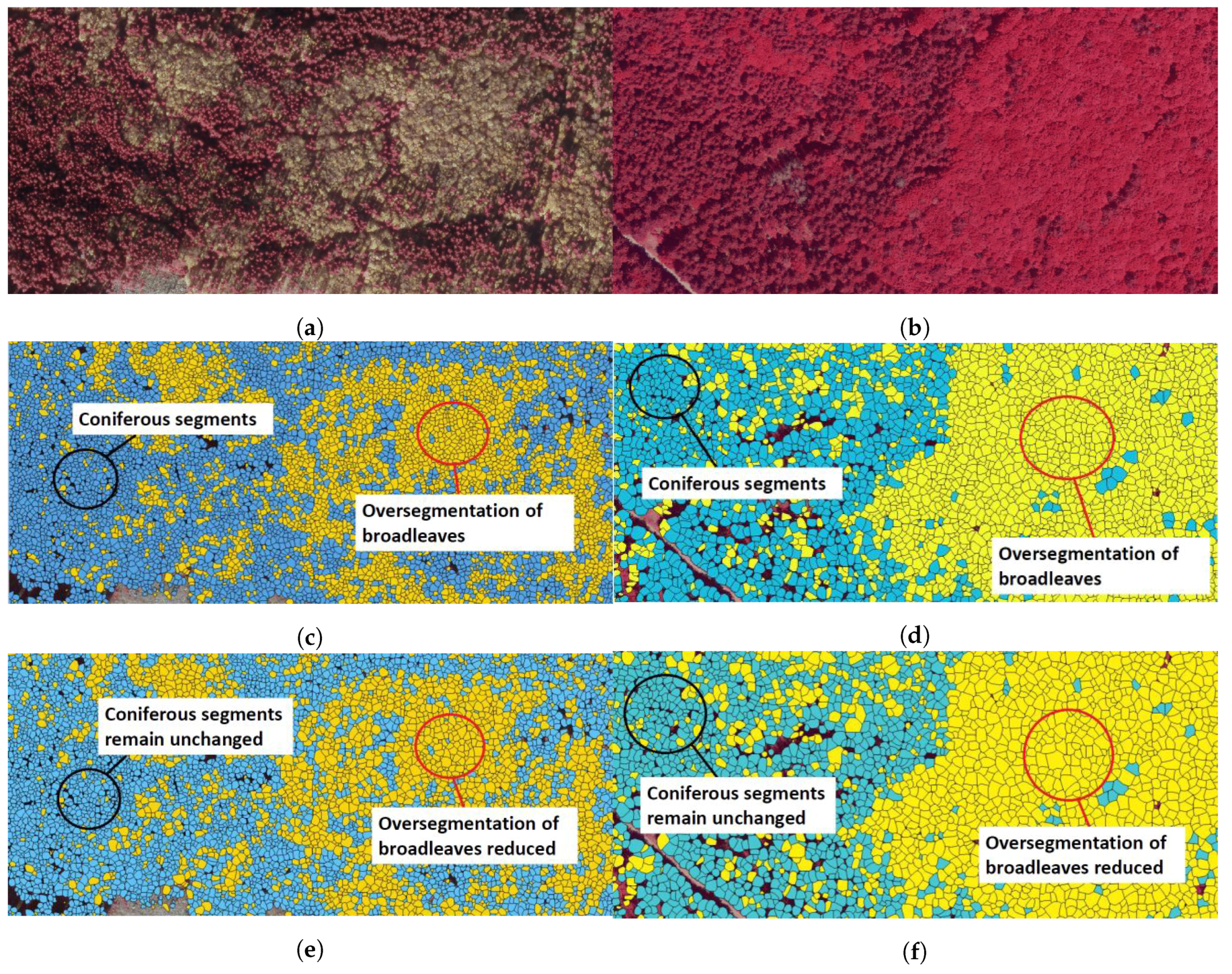
Figure 5.
Impact of parameter calibrated for conifers and broadleaf trees. Coniferous tree segments are in blue; broadleaf tree segments are in yellow. (a) Cut-out of aerial image in forest area of Šumava National Park. Approximate location is 48°47′57″N, 13°51′27″E. Approximate size is 655 m × 310 m. (b) Cut-out of aerial image in forest area of Bavarian Forest National Park. Approximate location is 48°55′45″N, 13°20′15″E. Approximate size is 456 m × 216 m. (c) Tree segments in area (a) = 0.16. (d) Tree segments in area (b) = 0.16. (e) Tree segments in area (a) = 0.10. (f) Tree segments in area (b) = 0.10.
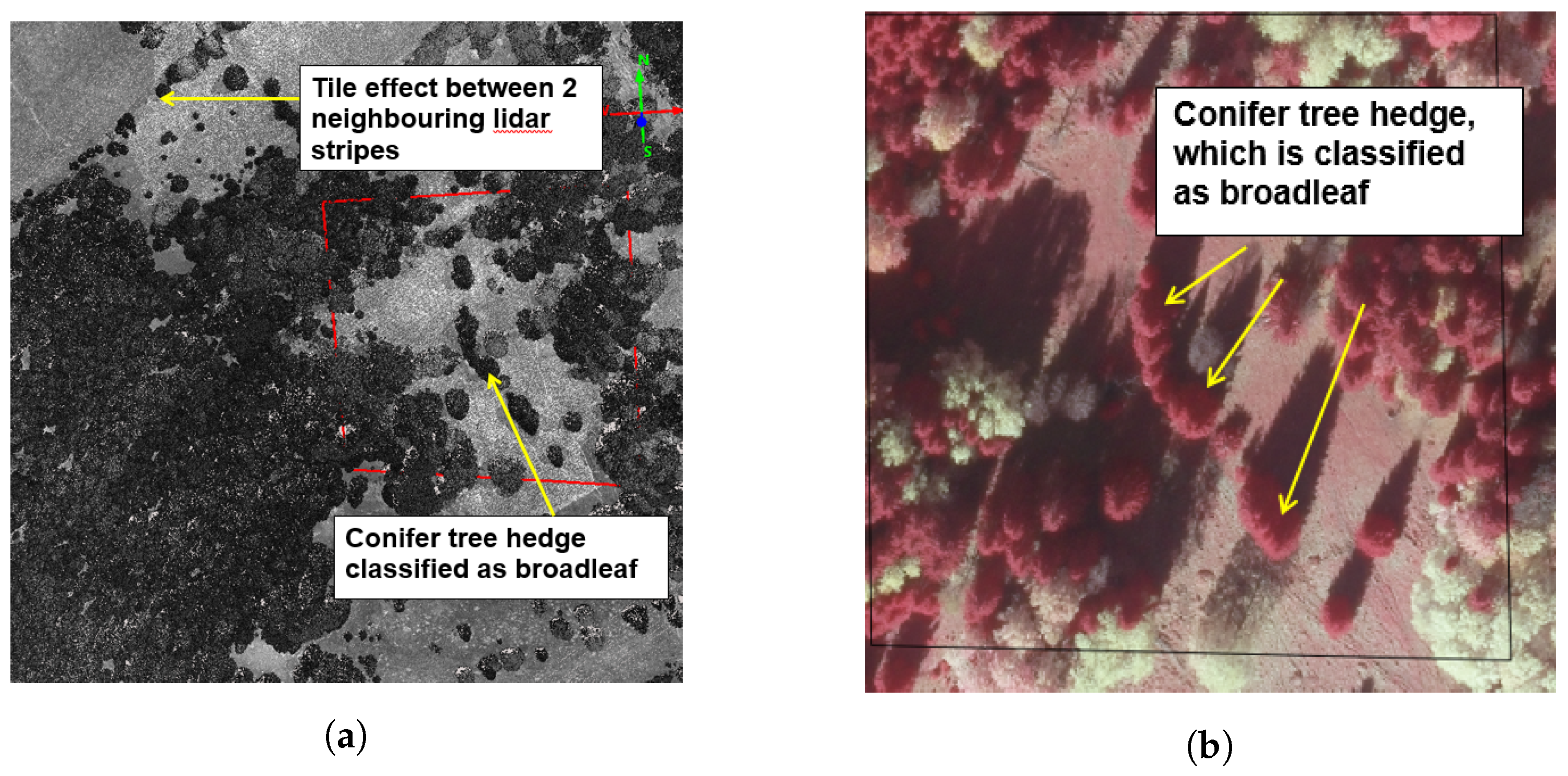
Figure 6.
Intensity issues in the mixed forest area. (a) Tile effect between neighboring laser strips (b) Mis-classified broadleaf trees.
Figure 6.
Intensity issues in the mixed forest area. (a) Tile effect between neighboring laser strips (b) Mis-classified broadleaf trees.
Figure 7.
Verification of the snag classifier in Bavarian Forest National Park. (a) Small forest scene with living trees, dead trees and snags. (b) Labelled snags for verification (green). (c) Classified snags (orange) with threshold > 90%.
Figure 7.
Verification of the snag classifier in Bavarian Forest National Park. (a) Small forest scene with living trees, dead trees and snags. (b) Labelled snags for verification (green). (c) Classified snags (orange) with threshold > 90%.
Figure 8.
Mapping of conifers, broadleaf trees, dead trees, and snags superimposed with orthophoto. Image source is from Bavarian Forest National Park.
Figure 8.
Mapping of conifers, broadleaf trees, dead trees, and snags superimposed with orthophoto. Image source is from Bavarian Forest National Park.
Table 1.
Flight parameters of lidar campaign.
Table 1.
Flight parameters of lidar campaign.
| Scanner Type | RIEGL LMS-680i |
|---|
| Platform | Helicopter |
| D-HFCE/AS350 |
| Spectral wavelength (nm) | 1550 |
| Beam divergence (mrad) | 0.5 |
| Flight speed (kts) | 60 |
| Flight height (m) | 550 |
| Side lap (%) | 60 |
| Point density (pts/m2) | 55 |
| Footprint size (mm) | 275 |
| Area (km2) | 943 |
| Number of raw laser points (Mio) | 52.400 |
Table 2.
Flight parameters of aerial image acquisition, results of subsequent aerial triangulation, and software packages used.
Table 2.
Flight parameters of aerial image acquisition, results of subsequent aerial triangulation, and software packages used.
| Park Area | Šumava | Bavarian Forest |
|---|
| Acquisition time | October 2017 | June 2017 |
| Aerial camera | Xp-w/a | DMCIII |
| End lap/Side lap (%) | 80/60 | 80/60 |
| Focal length (mm) | 100 | 92 |
| Number of images | 669 | 2553 |
| MSL flight height (m) | 3900 | 2880 |
| GSD (cm) | 17 | 9.5 |
| Sigma naught AT (GSD) | 0.22 | 0.3 |
| Software for AT | ISAT | MATCH-AT |
| Software for Orthophotos | OrthoMaster | OrthoMaster |
Table 3.
Properties of reference plots from field measurements.
Table 3.
Properties of reference plots from field measurements.
| Plot Areas | Bioklim CZ | HTO | Bioklim | LAI |
|---|
| Park area | Šumava | Bavarian Forest | Bavarian Forest | Bavarian Forest |
| Number of plots | 78 | 15 | 120 | 26 |
| plot size (ha) | 0.05 | ⌀ = 0.21 | 0.05 | 0.05 |
| Accuracy of plot centers | DGNSS | DGPS | DGNSS | DGNSS |
| Year of acquisition | 2017 | 2007 | 2016 | 2017 |
| Fir | 6 | 10 | 157 | 1 |
| Larch | 1 | 0 | 5 | 0 |
| Pine | 237 | 0 | 0 | 0 |
| Spruce | 1284 | 677 | 1397 | 6 |
| Alder | 12 | 0 | 16 | 0 |
| Ash | 2 | 0 | 2 | 37 |
| Beech | 354 | 883 | 1414 | 570 |
| Birch | 195 | 0 | 21 | 0 |
| Elm | 1 | 0 | 1 | 0 |
| Norway Maple | 0 | 2 | 0 | 0 |
| Rowan | 11 | 5 | 31 | 53 |
| Sycamore | 23 | 19 | 55 | 14 |
| Number of conifers | 1528 | 687 | 1559 | 7 |
| Number of broadleaf trees | 598 | 909 | 1540 | 674 |
| Conifers (%) | 72 | 43 | 50 | 1 |
| Broadleaf trees (%) | 28 | 57 | 50 | 99 |
| Total | 2126 | 1596 | 3099 | 681 |
| Forest type | coniferous | mixed | mixed | deciduous |
| Stem density (stems/ha) | 542 | 550 | 516 | 524 |
Table 4.
Properties of reference plots manually labelled.
Table 4.
Properties of reference plots manually labelled.
| Area | , , | , | |
|---|
| Year of acquisition | 2017 | 2017 | 2017 |
| Conifers | - | 4772 | 1796 |
| Broadleaf trees | - | 813 | 141 |
| Living trees | 1345 | - | - |
| Dead tree | 706 | - | - |
| Snag | 131 | - | - |
Table 5.
Control parameters of single tree segmentation.
Table 5.
Control parameters of single tree segmentation.
| Parameter | Symbols | Values |
|---|
| Min. number of super-voxels | | 2 |
| Weight for horizontal distance | | 1.35 m |
| Weight for vertical distance | | 11.0 m |
| Weight for stem position | | 3.5 m |
Table 6.
Control parameters of feature extraction with 3D shape contexts.
Table 6.
Control parameters of feature extraction with 3D shape contexts.
| Parameter | Symbols | Values |
|---|
| Cylinder radius | | 0.5 m |
| Cylinder length | | 2.0 m |
Table 7.
Sensitivity analysis for tree detection in reference areas. . Total number of trees is 1596.
Table 7.
Sensitivity analysis for tree detection in reference areas. . Total number of trees is 1596.
| Parameter | | Recall | | | | Precision | | |
|---|
| NCut | Lower | Middle | Upper | Total | Lower | Middle | Upper | Total |
| 0.13 | 0.16 | 0.38 | 0.84 | 0.64 | 0.23 | 0.53 | 0.67 | 0.58 |
| 0.16 | 0.18 | 0.41 | 0.90 | 0.69 | 0.20 | 0.51 | 0.62 | 0.54 |
| 0.18 | 0.19 | 0.44 | 0.92 | 0.71 | 0.23 | 0.52 | 0.60 | 0.52 |
| 0.20 | 0.24 | 0.45 | 0.91 | 0.72 | 0.21 | 0.50 | 0.58 | 0.49 |
Table 8.
Sensitivity analysis for tree detection in reference areas. HTO, Bioklim and LAI. Total number of trees is 5736.
Table 8.
Sensitivity analysis for tree detection in reference areas. HTO, Bioklim and LAI. Total number of trees is 5736.
| Parameter | | Recall | | | | Precision | | |
|---|
| NCut | Lower | Middle | Upper | Total | Lower | Middle | Upper | Total |
| 0.16 | 0.16 | 0.38 | 0.67 | 0.48 | 0.30 | 0.48 | 0.57 | 0.58 |
| 0.18 | 0.17 | 0.39 | 0.68 | 0.49 | 0.30 | 0.45 | 0.56 | 0.56 |
Table 9.
Sensitivity analysis for tree detection in reference areas. Bioklim CZ. Total number of trees is 2126.
Table 9.
Sensitivity analysis for tree detection in reference areas. Bioklim CZ. Total number of trees is 2126.
| Parameter | | Recall | | | | Precision | | |
|---|
| NCut | Lower | Middle | Upper | Total | Lower | Middle | Upper | Total |
| 0.16 | 0.13 | 0.37 | 0.67 | 0.51 | 0.29 | 0.56 | 0.70 | 0.73 |
| 0.18 | 0.13 | 0.36 | 0.67 | 0.52 | 0.28 | 0.53 | 0.69 | 0.72 |
Table 10.
Sensitivity analysis of tree detection regarding conifers and broadleaf trees. The reference area is . Control parameter = 0.16. Total number of trees is 1596.
Table 10.
Sensitivity analysis of tree detection regarding conifers and broadleaf trees. The reference area is . Control parameter = 0.16. Total number of trees is 1596.
| Parameter | | Recall | | | | Precision | | |
|---|
| Layer | Lower | Middle | Upper | Total | Lower | Middle | Upper | Total |
| Conifers | 0.10 | 0.53 | 0.89 | 0.69 | 0.27 | 0.66 | 0.85 | 0.82 |
| Broadleaf trees | 0.30 | 0.43 | 0.91 | 0.72 | 0.16 | 0.52 | 0.60 | 0.54 |
Table 11.
Sensitivity analysis of tree detection regarding conifers and broadleaf trees. The reference area is . Control parameter NCut = 0.10. Total number of trees is 1596.
Table 11.
Sensitivity analysis of tree detection regarding conifers and broadleaf trees. The reference area is . Control parameter NCut = 0.10. Total number of trees is 1596.
| Parameter | | Recall | | | | Precision | | |
|---|
| Layer | Lower | Middle | Upper | Total | Lower | Middle | Upper | Total |
| Broadleaf trees | 0.18 | 0.33 | 0.84 | 0.63 | 0.15 | 0.50 | 0.73 | 0.66 |
Table 12.
Results for the classification of conifers and broadleaf trees. Bavarian Forest National Park: Test data are from reference areas and : 1637 conifers and 636 broadleaf trees for training. 722 conifers, 253 broadleaf trees for testing (=Reference #1). 293 conifers, 236 broadleaf trees for testing (=Reference #2 only from ).
| | | Reference #1 | | | | Reference #2 | |
|---|
| Predicted | | Conifer | Broadleaf | Precision | Conifer | Broadleaf | Precision |
| Conifer | 687 | 15 | 0.98 | 269 | 44 | 0.85 |
| Broadleaf | 35 | 238 | 0.87 | 24 | 192 | 0.89 |
| Recall | 0.95 | 0.94 | | 0.92 | 0.81 | |
| | OA: 94.9% | Kappa: 0.87 | | | OA: 87.1% | Kappa: 0.89 | |
Table 13.
Results for the classification of conifers and broadleaf trees. Šumava National Park: Test data are from reference areas , and : 3480 conifers and 712 broadleaf trees for training. 1493 conifers, 314 broadleaf trees for testing (=Reference #3). 138 conifers, 187 broadleaf trees for testing (=Reference #4 only from ).
| | | Reference #3 | | | | Reference #4 | |
|---|
| Predicted | | Conifer | Broadleaf | Precision | Conifer | Broadleaf | Precision |
| Conifer | 1482 | 19 | 0.98 | 131 | 1 | 0.99 |
| Broadleaf | 11 | 295 | 0.96 | 7 | 186 | 0.96 |
| Recall | 0.99 | 0.94 | | 0.95 | 0.99 | |
| | OA: 97.5% | Kappa: 0.94 | | | OA: 97.5% | Kappa: 0.95 | |
Table 14.
Classification results of dead trees. Labelled data are from areas , , and . Bavarian Forest National Park: 124 dead trees, 186 living trees for training. 310 dead trees, 761 living trees for testing. Confusion matrices for training (left): Number of living trees are reduced to the number of dead trees. Numbers refer to the average of the five test sets of the five-fold cross-validation.
| | | Training Reference | | | | Test Reference | |
|---|
| Predicted | | Dead | Living | Precision | Dead | Living | Precision |
| Dead | 22 | 2 | 0.92 | 255 | 24 | 0.91 |
| Living | 2 | 22 | 0.92 | 55 | 737 | 0.93 |
| Recall | 0.92 | 0.92 | | 0.93 | 0.86 | |
| | OA: 91.7% | Kappa: 0.93 | | | OA: 92.6% | Kappa: 0.81 | |
Table 15.
Classification results of dead trees. Labelled data are from areas , , and . Šumava National Park: 163 dead trees with crowns, 356 living trees for training. 109 dead trees, 142 living trees for testing. Tree segments are classified as dead trees if the threshold for class probability > 90%.
| | | Training Reference | | | | Test Reference | |
|---|
| Predicted | | Dead | Living | Precision | Dead | Living | Precision |
| Dead | 27 | 6 | 0.82 | 109 | 0 | 1.0 |
| Living | 5 | 26 | 0.84 | 0 | 142 | 1.0 |
| Recall | 0.84 | 0.81 | | 1.0 | 1.0 | |
| | OA: 82.8% | Kappa: 0.65 | | | OA: 100.0% | Kappa: 1.0 | |
Table 16.
Results of the classification of snags for both parks. Labelled data are from areas A1, A2, and A3. 55 snags and 524 living trees for training. 76 snags and 1513 living trees for testing. Confusion matrices for training (left): Number of living are reduced to the number of snags. Numbers refer to the average of the five test sets of the five-fold cross-validation. Tree segments are classified as snags if the threshold for class probability > 90%.
| | | Training Reference | | | | Test Reference | |
|---|
| Predicted | | Snag | Living | Precision | Snag | Living | Precision |
| Snag | 10 | 1 | 0.91 | 50 | 39 | 0.56 |
| Living | 1 | 10 | 0.91 | 26 | 1474 | 0.98 |
| Recall | 0.91 | 0.91 | | 0.66 | 0.97 | |
| | OA: 90.9% | Kappa: 0.81 | | | OA: 95.9% | Kappa: 0.58 | |
Table 17.
Parameters and accuracy performance of tree segmentations methods compared with our study. Note that recall and precision values were evaluated from field measurements of plots.
Table 17.
Parameters and accuracy performance of tree segmentations methods compared with our study. Note that recall and precision values were evaluated from field measurements of plots.
| Study | Recall | Precision | Points/m2 | Trees/ha | Coniferous (%) | Deciduous (%) |
|---|
| Li et al. [40] | 0.86 | 0.94 | 6 | 400 | 100 | 0 |
| Strîmbu and Strîmbu [4] | 0.84 | 0.90 | 10 | 206 | 63 | 37 |
| Silva et al. [42] | 0.82 | 0.85 | 5 | 170 | 100 | 0 |
| Holmgren and Lindberg [41] | 0.85 | 0.82 | 83 | 626 | >50 | <50 |
| Our study (coniferous) | 0.89 | 0.85 | 55 | 550 | 100 | 0 |
| Our study (mixed) | 0.86 | 0.78 | 55 | 550 | 43 | 57 |
Table 18.
Number of classified trees.
Table 18.
Number of classified trees.
| Tree Type | Conifer | Broadleaf | Dead Trees | Snag |
|---|
| Šumava | 16.693.391 (=84%) | 2.396.850 (=12%) | 641.098 (=3%) | 224.533 (=1%) |
| Bavarian Forest | 4.446.373 (=60%) | 2.453.498 (=33%) | 312.058 (=4%) | 154.161 (=2%) |
Table 19.
Time performance of implemented algorithms.
Table 19.
Time performance of implemented algorithms.
| Process | Speed (sec/ha) |
|---|
| Tree segmentation | 25 |
| Classif. of conifers/broadleaf trees | 0.38 |
| Dead tree classification | 79 |
| Snag classification | 75 |

 ,
, 


