A Method for Underwater Acoustic Target Recognition Based on the Delay-Doppler Joint Feature

Abstract

With the aim of solving the problem of identifying complex underwater acoustic targets using a single signal feature in the Time–Frequency (TF) feature, this paper designs a method that recognizes the underwater targets based on the Delay-Doppler joint feature. First, this method uses symplectic finite Fourier transform (SFFT) to extract the Delay-Doppler features of underwater acoustic signals, analyzes the Time–Frequency features at the same time, and combines the Delay-Doppler (DD) feature and Time–Frequency feature to form a joint feature (TF-DD). This paper uses three types of convolutional neural networks to verify that TF-DD can effectively improve the accuracy of target recognition. Secondly, this paper designs an object recognition model (TF-DD-CNN) based on joint features as input, which simplifies the neural network’s overall structure and improves the model’s training efficiency. This research employs ship-radiated noise to validate the efficacy of TF-DD-CNN for target identification. The results demonstrate that the combined characteristic and the TF-DD-CNN model introduced in this study can proficiently detect ships, and the model notably enhances the precision of detection.

1. Introduction

The use of underwater acoustic signals for the purpose of identifying underwater targets has immense importance in the domains of marine resource exploitation and national defense security. The techniques for identifying underwater targets can be separated into two stages: extracting signal characteristics and developing an automated target classifier. The feature extraction method of early radiation noise is analyzed around the target energy spectrum and line spectrum characteristics. The continuous spectrum of the radiated noise may be accurately modeled using either the least square approach or power spectrum estimation. By eliminating the component of the continuous spectrum from the original signal, we can extract the line spectrum properties of the signal [1]. With the progress of neural networks, the energy spectrum features of underwater acoustic signals can be extracted using neural networks. As a relatively mature neural network, the Restricted Boltzmann machine can achieve high-precision extraction of ship target power spectrum features [2]. When examining underwater acoustic targets using signal time domain analysis, the cross-power spectrum obtained from coherence in the signal time domain may emphasize the distinctive line spectrum features of underwater targets [3]. The primary emphasis in the study of early underwater acoustic targets is on the temporal characteristics of the signal. However, the underwater acoustic signal is unstable and cannot accurately describe the signal characteristics in the time domain; so, the frequency domain of the signal can reflect the signal characteristics more stably. The double logarithmic spectrum feature is used to analyze the frequency domain features of ship radiation noise [4], and it improves the accuracy of target recognition. A single time domain or frequency domain feature contains less target feature information, and the Time–Frequency combined analysis can more comprehensively analyze the components of underwater acoustic signals that do not change with time. Wang et al. [5] extracted multi-beam low-frequency analysis and recording features, used convolutional neural networks to identify targets, and realized target detection. With the improvement of wavelet analysis technology, its excellent non-stationary signal analysis ability has received attention in the underwater acoustic field; so, it has been widely used in the analysis of radiation noise. Wavelet analysis is used to decompose underwater acoustic signals, and the wavelet coefficients extracted from the respective signals can reflect the characteristics of the target [6], which can not only improve the accuracy of the target recognition but also provide a new idea for signal denoising. The combination of empirical mode decomposition (EMD) and wavelet decomposition is used to remove noise from underwater acoustic targets, resulting in signals with a high ratio of signal to noise. This process enhances the accuracy of target detection [7]. With the development of the chaos theory and nonlinear dynamic principle, it is frequently applied to the characteristic analysis of underwater acoustic targets. Refined composite multiscale fluctuation-based dispersion entropy (RCMFDE) is proposed to extract ship features, and the experimental results show the validity and universality of the classification [8]. Combined with improved intrinsic time-scale decomposition (IITD) and multiscale dispersion entropy (MDE), it can significantly raise target recognition accuracy [9]. The majority of the aforementioned feature extraction techniques concentrate on the signal’s Time–Frequency domain features. The overlapping feature frequency ranges of various underwater acoustic targets provide an immediate challenge in accurately identifying the target when using the signal’s characteristics in the Time–Frequency domain as a result of the fast progress in oceanic technology.

In order to solve the problem that it is difficult to recognize more complex targets by using time-frequency feature, this paper analyzes the signal from the perspective of Delay-Doppler domain. The motion characteristics of the target are defined by the Delay-Doppler domain components of the signal. Because of the difference in volume and shape, the velocity of different underwater acoustic targets is quite different. The Delay-Doppler features can represent the difference of targets within a specific range. The coherence integration method of the power spectrum is used to compensate for the Delay-Doppler factor of passive sonar signals, which may significantly enhance the detection efficacy of mobile targets [10]. The underwater acoustic communication receiver has a high bit error rate (BER) since it was constructed using the signal characteristics found in the Delay-Doppler feature [11]. The accuracy of signal features may be increased by using deep learning for the feature extraction of signals in the Delay-Doppler domain as the field develops and advances [12]. The Delay-Doppler features of signals are widely used in underwater acoustic communication. Sun et al. [13] proposed an orthogonal operation based on the Gram–Schmidt method to solve the multi-path sparse Delay-Doppler parameter solution of linear frequency modulated (LFM) signals in shallow water. Compared to the traditional method, it has a lower mean square error. Guo et al. [14] introduced exponential modulation (IM) into the Delay-Doppler feature of the signal, and the system’s BER performance was enhanced by using the Hamming distance optimization model. Zhang et al. [15] created a generalized approximated message passing (GAMP) algorithm to estimate underwater acoustic channels in a communication system, which can effectively reduce the computational complexity. The signal’s Delay-Doppler characteristics can reflect the target’s motion characteristics. However, the target’s speed varies over time and cannot stably reflect the characteristics of the target. This study combines the temporal and spectral properties of the signal to address the aforementioned problem. By using the Time–Frequency feature and the Delay-Doppler feature together, it is possible to mitigate target identification mistakes that may occur when utilizing these features individually. Instead, it suggests an approach to target feature extraction that is based on both domains.

Automatic recognition and classification technology are essential to realize the intelligence and automation of underwater acoustic equipment. The early recognition of underwater targets mainly relies on experienced professionals. With the progress of computers and related algorithms, there have been some target recognition methods based on statistical analysis, such as the Bayesian pattern classification method, cluster analysis method, support vector machine, restricted Boltzmann machine, decision tree, hidden Markov model, and nearest neighbor method [16] using wavelet packet transform to process the signal, extract the wavelet energy spectrum features of the radiated noise signal, and use SVM to identify the signal effectively. Spampinato et al. [17] used the hidden Markov model to compare the trajectory of underwater fish and realize the trajectory detection of underwater fish. Luo et al. [18] used a restricted Boltzmann machine to examine the normalized spectrum of the signal, obtain the data’s deep structural features, and finally classify the data with BP neural network features. With the emergence of artificial intelligence, there is increasingly more research on recognizing underwater acoustic targets using neural networks. Convolutional neural networks (CNNs) are often used for underwater target detection. Song et al. [19] extracted five characteristic parameters of radiated noise in the frequency, time, and Mel transform domains and established a convolutional neural network to recognize the target. The recognition accuracy was improved by 7.8% compared to the SVM method. Hu et al. [20] established an extreme learning machine to recognize the signal by using a deep neural network to extract characteristics of radiated noise, and the identification accuracy was 93.04%. Wang et al. [21] extracted the modified empirical mode decomposition and gamma tone frequency cepstrum coefficient of the signal, and fused the two signal features into new features. The deep neural network’s structure is optimized using the Gaussian mixture model, and the target is recognized by the optimized deep neural network. With the iterative progress of computer technology, artificial intelligence technology represented by deep learning will be more widely used to recognize and classify underwater target radiation noise. Using neural networks to identify underwater acoustic targets can significantly reduce labor costs, and it is an area for significant future development in this field. The traditional neural network model has the disadvantage of complex model structure, which can not be well used in underwater acoustic target recognition.

In this work, to thoroughly examine the target’s characteristics from two angles, we first propose a feature extraction method that utilizes the Delay-Doppler and Time–Frequency domains. Then, this research introduces a target recognition network specifically tailored for the proposed feature extraction approach. Our structure is more straightforward than traditional neural network models, with no overfitting or underfitting problems. The innovative contributions of this study are outlined below:

• This work suggests a joint feature identification method that is based on the Delay-Doppler and Time–Frequency domains. The purpose of this method is to analyze ship-radiated noise from a new perspective of signal processing and provide a new basis for underwater acoustic target recognition. The algorithm extracts signal characteristics that include a broader range of target information.
• This research presents a target recognition model that uses joint features in conjunction with a convolutional neural network (TF-DD-CNN). This model streamlines the model architecture and enhances the efficacy of model training. The experimental findings demonstrate that its recognition accuracy surpasses that of the conventional neural network model.

2. Theory

2.1. Time–Frequency Domain Analysis

The hydrophone captures a time-varying discrete signal that represents the radiated noise data of the underwater target, which shows the time-varying information of sound pressure. The single time domain information can not reflect the time-varying signal’s characteristics; so, the signal’s frequency domain characteristics need to be analyzed. If the radiated noise signal is denoted as $p\left(n\right)$, the formula in the frequency domain after performing the discrete Fourier transform (DFT) is given by [22]:

$$P{\left(\omega \right)}_k={\displaystyle \sum }_{n=0}^{N-1}p\left(n\right)e^{-j\frac{2\pi }{N}nk}$$

(1)

In this formula, $P{\left(\omega \right)}_k$ is the frequency, 0 ≤ k ≤ N − 1 and N is the total length of the signal. The discrete Fourier transform is capable of transforming the sound pressure signal $p\left(n\right)$ into its corresponding representation in the frequency domain, denoted as $P\left(\omega \right)$. Because of the intricacy involved in computing the discrete Fourier transform and the limited ability to accurately resolve low-frequency components, the fast Fourier transform has been developed. Compared to the traditional Fourier transform algorithm, the FFT algorithm can significantly reduce the computational load and improve the computational efficiency [23].

The hydrophone captures the radiation’s noise signal, which is then divided into several frames for processing. Then, each data frame is windowed to improve the spectral characteristics of the signal and reduce the spectral leakage. FFT obtains the spectrum characteristics of each frame of a windowed signal, and then the signal is processed in the time and frequency domains. The frequency is shown on the vertical axis, while the horizontal axis represents time. The signal’s amplitude is represented by color filling, and the Time–Frequency characteristics are obtained after the above processing. Figure 1 shows the specific Time–Frequency domain acquisition process. The Time–Frequency feature can show the frequency band of the signal that does not change with time, which is an essential reference for target identification.

2.2. Delay-Doppler Domain Analysis

The Doppler effect occurs when there is relative motion between the target and the receiver in the received acoustic signal. This motion causes a change in the frequency of the signal, which can be analyzed using the Delay-Doppler feature analysis. Therefore, the Delay-Doppler domain feature of the signal can represent the motion characteristics of the target. The velocity intervals of underwater acoustic targets with different shapes and sizes are often significantly different; so, they can show different characteristics in the Delay-Doppler feature. This research aims to analyze the Delay-Doppler features of underwater acoustic signals and use them for the purpose of distinguishing various underwater acoustic objects. The signal’s Time–Frequency and Delay-Doppler domain components are interconnected and may be modified using the symplectic finite Fourier transform (SFFT) and its inverse transformation (ISFFT). The connection between the discrete signal’s features in the Time–Frequency, Delay-Doppler, and time domains is shown in Figure 2.

The discrete sound pressure signal s(n) is acquired by fast Fourier transform (FFT), as seen in Figure 2. The symplectic finite Fourier transform (SFFT) may be used to extract the pertinent Delay-Doppler information from s(n). The formula of SFFT is as follows [24]:

$$Y\left[m,n\right]=\frac{1}{\sqrt{MN}}{\displaystyle \sum }_{l=0}^{M-1}{\displaystyle \sum }_{k=0}^{N-1}{X}_{tf}\left[l,k\right]e^{-j2\pi \left(\frac{nk}{N}-\frac{ml}{M}\right)}$$

(2)

In the above formula, the matrix $Y\left[m,n\right]$ represents the eigenvalues of the signal in the Delay-Doppler domain, where m = 0, 1, …, M − 1; n = 0, 1, …, N − 1. M represents the quantity of grid points in the time domain, whereas N represents the number of grid points in the frequency domain. SFFT is computed by performing the discrete Fourier transform (DFT) on the N-point and then by applying the inverse discrete Fourier transform (IDFT) on the M-point.

Figure 3 illustrates the connection between the Delay-Doppler and Time–Frequency domains. The conversion connection between the Doppler domains and time is shown by the horizontal axis. The use of the DFT enables the transformation from the time domain to the Doppler domain. The relationship between the frequency domain and the delay domain is shown by the vertical axis, and the transformation from the frequency domain to the delay domain is achieved using IDFT. The alteration in frequency resulting from the relative movement between objects is referred to as the Doppler effect. Consequently, the Doppler domain may be interpreted as the characteristic of the target’s velocity, and the target’s motion characteristic can be derived by analyzing the signal delay in the Doppler domain. The variation in speed among distinct targets might serve as a distinguishing characteristic for target identification.

2.3. Convolutional Neural Network

A basic convolutional neural network (CNN) consists of an input layer, a convolutional layer, a pooling layer, a fully connected (FC) layer, and an output layer. The convolutional layer has three main functions: it extracts features from the input data, minimizes the number of deep learning parameters, and maintains the input data space. The complete convolutional neural network structure is shown in Figure 4. Convolution kernel size f, convolution kernel move step s, and convolution kernel number filter are some of the fundamental parameters that make up the convolution layer’s basic structure. To determine the output value of the window, the convolution kernel is applied in the 6 × 6 window that corresponds to the input data. The count of convolution kernel skips in the input matrix is known as the moving step. The convolution kernel window moves s units to carry out the convolution operation on the corresponding window data again, and the convolution data are obtained after traversing and convolutioning all the input data.

The convolution process essentially multiplies the elements between the convolution kernel and the corresponding input data and finally sums all multipliers. $X_{ij}$ and $K_{ij}$ are the values of the input data and the convolution check, and R is the convolution data. The precise formula is as follows:

$$R={\displaystyle \sum }_{i=1}^n{\displaystyle \sum }_{j=1}^n{X}_{ij}{K}_{ij}$$

(3)

The data are processed using convolution and pooling layers, and then, an FC layer is used to minimize the dimensionality of the data and create the feature matrix. Next, the SoftMax layer is used to categorize and recognize the feature matrix. The SoftMax layer is a classifier used for deep learning. It can map the output classification result to the range of zero to one. The likelihood that the sample will belong to the class is represented by the probability of the output-related result. The SoftMax layer is the classification layer of the CNN. Let n be the number of target categories to be classed and identified. The output vector obtained through the FC layer is $f\left(x\right)$. The output result of the SoftMax layer is shown in Formula (4) [25], where $p_i\left(x\right)$ represents the output probability of the i type of target and $f_i\left(x\right)$ represents the output vector of the target FC layer of type i. Finally, SoftMax selects the target with the highest probability $\left\{p_i\right\}$ as the output value of the signal, which is the label of the target identified by the model.

$$p_i\left(x\right)=\frac{e^{f_i\left(x\right)}}{{{\displaystyle \sum }}_{j=1}^n{e}^{f_j\left(x\right)}},i=1,2,\dots ,n$$

(4)

The process of convolution and pooling is essentially a process of feature extraction and data compression. The selection of a convolution kernel with different attributes can extract different dimensional data information. Therefore, the CNN is a kind of network widely used in classification.

3. Underwater Acoustic Target Recognition Model with Delay-Doppler Joint Feature

3.1. Time–Frequency and Delay-Doppler Features of Ship-Radiated Noise

This section mainly introduces the Time–Frequency and Delay-Doppler features of ship-radiated noise. This paper examines the ship-radiated noise signal using FFT and extracts the frequency characteristics of ship-radiated noise. The primary sources of ship-radiated noise are vibration noise, propeller noise, and cavitation noise from bubbles. Vibration noise and propeller noise are the most significant, and ship-radiated noise is mostly low-frequency noise below 500 Hz [26]. Figure 5 shows the time domain feature of an Oceanliner’s radiated noise, while Figure 6 shows the frequency domain feature of the target. Figure 6 illustrates that the signal frequency is mostly focused below 1 kHz, with the largest amplitude occurring at around 50 Hz. Figure 7 is the Time–Frequency feature of the ship, as shown by the red line in the figure; most of the signal’s energy is concentrated in the frequency band below 1000 Hz. A comparison of Figure 6 to Figure 7 reveals that the ship’s data are mostly focused in the low-frequency range below 1000 Hz, and the frequency distribution is unaffected by temporal variations.

The Delay-Doppler feature of the underwater acoustic signal can be obtained by using the Time–Frequency domain feature through SFFT conversion. Because the fast Fourier transform exhibits symmetry, the Delay-Doppler feature of the signal also exhibits symmetry. Therefore, it is sufficient to study just the first half of the signal’s data. Figure 8 is the Delay-Doppler feature image corresponding to the Oceanliner’s data. The Figure 8 shows a Doppler frequency shift near 20 Hz, and the signal’s speed feature may be reflected in the image. Figure 9 shows a three-dimensional display of the Delay-Doppler characteristics, which can more intuitively reflect the Delay-Doppler feature information of the signal. The speed feature of the target can be obtained by using the propagation speed and Doppler frequency shift of acoustic waves in a seawater medium. The signal’s Delay-Doppler characteristic information can be reflected more directly.

The signal’s Time–Frequency domain feature depicts the target’s intrinsic characteristics, and the signal’s properties remain relatively constant throughout time. The target’s velocity characteristics, or its dynamic characteristics, may be reflected in the signal’s Delay-Doppler feature. The speed range of different targets is different. For example, torpedoes can reach more than 60 knots per hour, speedboats can reach about 40–60 knots per hour, ordinary fishing boats can reach about 10–15 knots per hour, and large oil tankers can reach less than 10 knots per hour in ports. The targets of different sizes and functions have corresponding speed ranges; so, speed can be used to roughly divide target types.

Figure 10 shows the idea of using the above two signal features as the basis for classification in this paper. Since different targets have different shapes and sizes, their speed ranges are also different; so, they have different features in the Delay-Doppler domain. Targets may be categorized into several speed ranges based on the target signal’s Delay-Doppler properties, and the target size may be determined by analyzing the speed properties of the signal. The radiated noise generated by different targets may have frequency overlap; so, only depending on the signal’s Time–Frequency features to identify the target is challenging. The properties of the target from another feature domain of the signal may be described by the Delay-Doppler feature, and the foundation of the classification is the joint features that combine the Time–Frequency and Delay-Doppler features. The dimension of the description signal is increased, which can reflect the target information more comprehensively.

3.2. Target Recognition Model with Time–Frequency and Delay-Doppler Features

This paper establishes a multi-input underwater acoustic target recognition model (TF-DD-CNN) based on Time–Frequency features and Delay-Doppler features of underwater noise emitted by ships. The model consists of a Time–Frequency feature recognition module and a Delay-Doppler domain feature recognition module, and uses a convolutional neural network to construct the target recognition model. The particular arrangement is seen in Figure 11. The model structure mainly comprises the Time–Frequency (TF) feature recognition model and the Delay-Doppler (DD) feature recognition model. Each module consists of nine groups of convolution modules (Conv k, k = 1, 2, …, 9). The feature vector matrix finally obtained by the two modules is fused by the Feature Fusion module, and the high-dimensional and complex signal features are converted into low-dimensional and simple signal features by using two sets of fully connected layers. Finally, the SoftMax layer is used to identify the target, and the network architecture employs cross entropy as the loss function for model training.

Table 1. Parameter settings of the convolutional module.

Convolutional Module	Parameter Settings
Conv 1	1 × 1-Conv2D-32-ReLu-BN; 3 × 3-MaxPooling
Conv 2	1 × 1-Conv2D-32-ReLu-BN; 3 × 3-MaxPooling
Conv 3	3 × 3-Conv2D-32-ReLu-BN; 3 × 3-MaxPooling
Conv 4	1 × 1-Conv2D-32-ReLu-BN; 3 × 3-MaxPooling
Conv 5	5 × 5-Conv2D-32-ReLu-BN; 3 × 3-MaxPooling
Conv 6	1 × 1-Conv2D-64-ReLu-BN; 3 × 3-MaxPooling
Conv 7	5 × 5-Conv2D-64-ReLu-BN; 3 × 3-MaxPooling
Conv 8	1 × 1-Conv2D-64-ReLu-BN; 3 × 3-MaxPooling
Conv 9	5 × 5-Conv2D-64-ReLu-BN; 3 × 3-MaxPooling

displays the comprehensive details of each convolutional layer in the model. In order to add nonlinear conditions to the model, the activation function used to train the model is the Rectified Linear Unit (ReLU), and the pooling layer of each layer is selected as MaxPooling. We take Conv1 as an example to explain the contents in Table 1. The notation “1 × 1-32-ReLu-BN” indicates that the chosen convolution kernel has a size of 1 × 1, the type of convolution kernel is a two-dimensional convolution kernel, 32 represents the number of convolutions, and the selected activation function is the ReLU. Batch Normalization (BN) [27] is a data normalization method. It can accelerate the convergence rate of model training and improve its robustness; “3 × 3-MaxPooling” indicates that the selected pooling size is 3 × 3, and the maximum pooling is selected for processing.

The input feature vector passes through nine convolutional layers to obtain the corresponding convolutional feature vector. Finally, we use the Feature Fusion module to merge the two categories of convolutional feature vectors. The process of fusion is referred to as matrix concatenation, and Figure 12 shows the precise fusion process. Assuming that both input vectors are m × n matrices, the Feature Fusion module is used to obtain a 2m × n feature vector at last. Suppose the number of columns of the two feature matrices is inconsistent. In that case, the corresponding column number of the feature matrix with fewer columns will be zeroized and then fused, which will be used as the basis for the final target recognition. The dimensionality of the matrix is reduced using two completely linked layers, and the SoftMax layer is then utilized for identification.

4. Experiment

The Time–Frequency and Delay-Doppler characteristics provide the ability to comprehensively represent the information of the target. In this paper, the two signal features were composed of joint features to recognize the target, and the CNN approach was used for recognizing the underwater targets. A multi-input feature target recognition network structure was designed, and the combined Time–Frequency and Delay-Doppler properties of signals were used to identify the targets. To assess the efficacy of the proposed combined features and recognition network model for target recognition, several mature CNNs were also constructed: the VGG16, GoogleNet, and ResNet models were used to validate the new recognition model by assessing the classification accuracy of several recognition models.

4.1. Experimental Environment Configuration

This section provides an overview of the experimental environment, specifically focusing on the configuration of the computer hardware and software versions used in the experiment. It explains how the environment might impact the pace at which the model is trained. The graphics processing unit (GPU) was the NVIDIA GeForce RTX 4080 (NVIDIA, Santa Clara, CA, USA), while the central processing unit (CPU) was the Intel i9-13900K (Intel, Santa Clara, CA, USA). To enhance the efficiency of model training, the neural network underwent training using a GPU. The computer’s operating system was Windows 10, with a total RAM capacity of 128 GB. In this study, a predictive model was constructed using the Python programming language, specifically Python version 3.9. The neural network was constructed using the PyTorch framework. The Pycharm2018 compiler was used for the implementation.

4.2. Data Introduction and Preprocessing

The data used in this paper were sourced from the ShipsEar database, which can be consulted online at http://atlanttic.uvigo.es/underwaternoise/, accessed on 1 November 2023. The hydrophone that collected these data was moored on the seafloor and connected to an underwater buoy to ensure a vertical position, and the upper end was connected to a surface buoy [28]. The database comprises 11 distinct categories of ship radiation noise data, as well as a collection of marine environmental background noise data. The data are stored in audio format, and Figure 13 is a time domain waveform of the first 20 s of a passenger ship in this database. Since the collection time of each ship is different, the total data duration of each type of ship is also different. This paper uses data from the four longest collected ship types and marine environmental noise as targets.

The recognition model trained using only the ShipsEar database was not convincing; so, the author’s research group collected a set of radiated noise data from fishing boats, passenger ships, and motorboats to verify the effectiveness of the model. The data collection site is located at Jimiya Port in the West Coast New Area in Qingdao City. The port is busy with freight transportation and has a large number of different types of ships entering and exiting the port all day. When we collected these data, the wind and waves were low; so, the impact of marine environmental noise on the data is relatively small. Figure 14 shows images of some targets in the ShipsEar database and data collected by the research team.

Table 2. Information of radiated noise signal.

Type	Number of Samples	Total Duration (s)
RO-RO Ship	5	1512
Oceanliner	7	938
National Noise	12	1134
Motorboat	13	1008
Passenger Ship	30	4256

shows the target types and data duration of the data used in this article. These targets have significant differences in size, making them suitable for analyzing the target recognition performance of Delay-Doppler features based on them.

Figure 15 shows the preprocessing process of the original data in this paper, with the aim of obtaining Time–Frequency and Delay-Doppler features for target recognition and using these two features as training sets to train the recognition model (TF-DD-CNN). First, this paper frames the original data to expand the data volume. Second, FFT is used to analyze the frequency domain features of the processed data, combined with the time domain feature to form the Time–Frequency feature. Third, SFFT is used to analyze the Delay-Doppler feature of the data. Finally, this paper uses the Time–Frequency and Delay-Doppler features of the signal to create training data for the TF-DD-CNN. The ratio of the number of training and testing sets is set to 5:1.

This research applies frame processing techniques to the original radiation noise data in order to enhance the training set. Figure 16 depicts the process of dividing the radiation noise signal into frames. The length of the radiated noise signal is denoted as n, data frame length (DFL) indicates the length of the intercepted signal, where DFL < n, and frame shift (FS) indicates that every few groups of data start to intercept the next frame of data. In this paper, the original data are divided into two frames, and the radiation noise data are divided into one frame every two seconds. To ensure the seamless flow of information between neighboring data frames, the overlap rate of adjacent data will be maintained by 50%. To meet the need for a 50% overlap rate, the step size can be selected as half of the DFL; the frameshift is one second. Figure 17 is the time domain diagram of a four-frame signal of certain data, with one frame of data every two seconds and the step size set to one second so that the data of two adjacent frames has a 50% overlap rate.

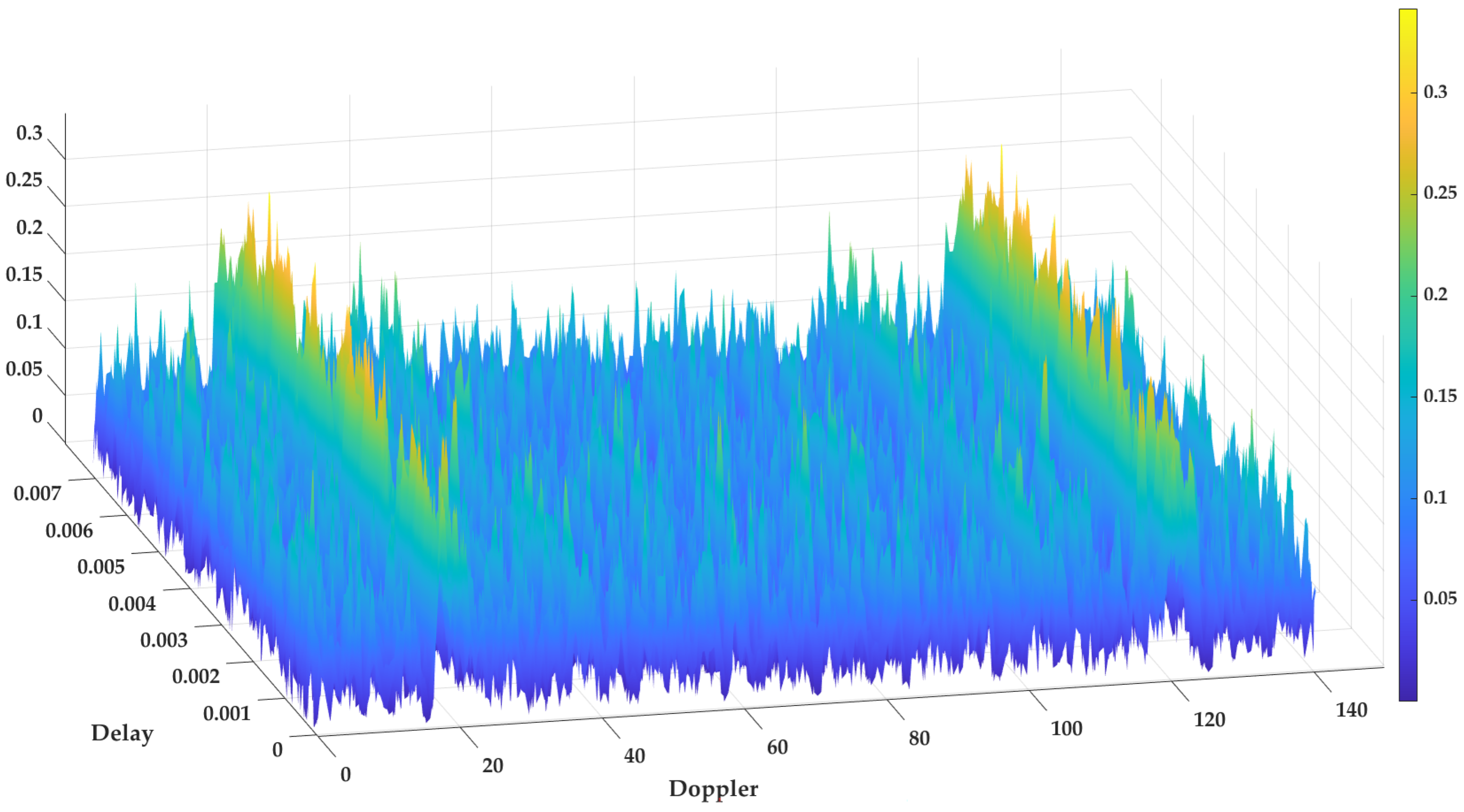
Figure 18 shows the Time–Frequency and Delay-Doppler features of a passenger ship. Figure 18a shows the Delay-Doppler feature of the ship and Figure 18b shows the Time–Frequency feature of the ship, with the signal energy mainly concentrated in the low-frequency band. From the analysis of the Figure 18a, the target has a relatively obvious Doppler frequency shift. In order to improve the accuracy of target recognition, all coordinate information is hidden from the input results.

4.3. Evaluation Criteria for Target Recognition Results

This study employed four metrics, namely, accuracy, precision, recall, and F1 Score [29], to assess the experimental outcomes. Accuracy (Acc) is a measure that calculates the ratio of correctly predicted samples by the classification model to the total number of samples. It provides a measure of the overall prediction accuracy of the model across all samples. Precision (Pre) is the quotient obtained by dividing the number of accurately anticipated positive samples by the total number of samples predicted as positive. It measures the precision of the model’s predictions for the positive category. Recall (Rec) is the quotient obtained by dividing the number of accurately predicted positive category samples by the total number of actual positive category samples. It quantifies the rate at which the model correctly identifies positive category samples. The F1 score (F1) is a metric that quantifies the balance between prediction accuracy and recall by calculating their harmonic mean. It considers both aspects to provide a comprehensive evaluation of the model’s performance. For multi-classification problems, the construction of the confusion matrix can be shown in

Table 3. Confusion matrix of multiple categories.

	Actually Positive	Actually Negative
Predicted as positive	PP	PN
Predicted as negative	NP	NN

.

$$Acc=\frac{PP+NN}{PP+PN+NP+NN}$$

(5)

$$Pre=\frac{PP}{PP+PN}$$

(6)

$$Rec=\frac{PP}{PP+NP}$$

(7)

$$F1=\frac{2\times Pre\times Rec}{Pre+Rec}$$

(8)

Among the four sets of formulas, PP is the count of positive recognition outcomes from the recognition model, where the actual label is also positive. PN denotes the count of recognition outcomes from the model that is accurate, but the corresponding true label is incorrect. NP denotes the count of recognition results from the recognition model that is incorrect, while the actual label is correct. NN represents the number of recognition results from the recognition model that are both false and have a false actual label. The formulas for accuracy, precision, recall, and F1 score are derived from the confusion matrix.

4.4. Results and Analysis

This study performed two sets of tests to validate the accuracy of the Delay-Doppler domain features and the multi-input target recognition model (TF-DD-CNN). In experiment 1, signals’ Time–Frequency domain features (TF), Delay-Doppler domain features (DD), and joint features (TF-DD) were respectively used as inputs. The joint features of signals were realized using Feature Fusion in Figure 12. The VGG16 model, ResNet model [30], and GoogleNet model [31] were used for target recognition to verify the effectiveness of Delay-Doppler domain features for target recognition. The objective of experiment 2 was to validate the efficacy of the developed recognition model by using the TF-DD-CNN model to identify the target and assess the accuracy of various models.

4.4.1. Joint Feature Recognition Experiment

Experiment 1 verified the effectiveness of Delay-Doppler domain features for target recognition. The joint features were obtained based on the Feature Fusion method in Figure 12, which takes the Time–Frequency feature and Delay-Doppler feature of the signal as inputs and uses the Feature Fusion method to obtain the joint features. This experiment could verify that the joint features can effectively improve the accuracy of target recognition compared to a single Time–Frequency feature. Figure 19 shows the overall image of the loss function obtained from all nine groups of the experiments. The icon represents the combination of network structure and input features. The term “VGG-TF” refers to the outcome of employing the VGG model with Time–Frequency feature recognition. Similarly, “VGG-DD” denotes the result of using the VGG model with Delay-Doppler feature recognition. Lastly, “VGG-TF-DD” signifies the outcome of utilizing the VGG model with joint feature recognition. Each set of experiments conducted 70 rounds of training. The learning rate was set to 0.001, and the ratio of training sets to test sets was defined as 5:1.

Table 4. Experimental identification results of each group.

Models	Acc (%)	Pre (%)	Rec (%)	F1 (%)
VGG-TF	63.94/72.83	63.42/72.83	63.94/72.83	63.23/72.40
VGG-DD	61.60/68.58	60.78/70.60	61.59/68.57	60.51/67.15
VGG-TF-DD	69.60/77.08	69.10/78.32	69.60/77.08	69.14/76.26
ResNet-TF	75.84/72.09	75.58/72.39	75.84/72.09	75.48/71.98
ResNet-DD	71.06/67.95	70.60/67.42	71.06/67.95	70.38/67.31
ResNet-TF-DD	80.37/79.30	80.08/79.09	80.37/79.30	80.09/79.12
GoogleNet-TF	70.53/70.73	70.22/70.82	70.53/70.73	70.01/70.71
GoogleNet-DD	64.07/64.21	63.20/64.79	64.07/64.21	62.93/62.60
GoogleNet-TF-DD	72.86/73.79	72.34/74.66	72.86/73.79	72.23/73.71

displays the outcomes of Acc, Pre, Rec, and F1 achieved by each experimental group. The table shows the results of “Training set results/ Testing set results”, and Figure 20 exhibits the recognition accuracy outcomes of the three models on the training set.

The findings of experiment 1 confirm that the use of Delay-Doppler features significantly enhances the accuracy of ship target detection. Figure 19 shows that the three models’ accuracy is best after 30 training iterations. Table 4 shows that the recognition accuracy of several models is between 60% and 80%, among which the ResNet model has the best recognition effect. Figure 20 displays the distribution of identification accuracy for various recognition models and input characteristics. Figure 20 demonstrates that the ResNet network has the highest recognition accuracy, and the recognition results obtained by analyzing the different feature inputs of each model with joint features as the basis are the highest, followed by Time–Frequency domain features. The lowest recognition accuracy is the Delay-Doppler feature, which also reflects the idea proposed in Section 3.1 of this paper. To a certain extent, the result distribution of Figure 20 proves the analysis of Figure 10 because Delay-Doppler may contain multiple overlapping target features, and the corresponding recognition accuracy will be lower than the Time–Frequency domain features. However, by combining the two features, the recognition accuracy of the final model will be greatly enhanced. By analyzing the results of Figure 20 and Table 4, the use of the joint feature (TF-DD) described in this research leads to an average increase in target identification accuracy of around 6–8% compared to employing a single feature alone. This gain is rather noticeable.

4.4.2. TF-DD-CNN Model Target Recognition Experiment

Experiment 2 aimed to validate the efficacy of the network model that was constructed. Experiment 1 provided the recognition results of joint features (TF-DD) by the VGG model, ResNet model, and GoogleNet model; so, Figure 21 only displays the training loss function of the TF-DD-CNN model, while the model’s recognition accuracy outcomes are shown in

Table 5. Recognition results of the TF-DD-CNN model.

Dataset	Acc (%)	Pre (%)	Rec (%)	F1 (%)
Training sets	93.56	93.64	93.57	93.60
Testing sets	92.23	92.34	92.23	92.28

. Figure 22 shows the prediction accuracy of the VGG, ResNet, GoogleNet, and TF-DD-CNN models.

Figure 21 shows the curve of the loss function changing with the number of training iterations. The loss function of the model reaches its lowest level after 15 training iterations, and the training efficiency is higher than the three models in Section 4.4.1. This efficient training performance benefits from the simple model structure, which reduces the computational burden during the model training process. From Table 5, it can be seen that in the recognition results of the training set, the multi-input recognition model can achieve a recognition accuracy of 94%, and it can also achieve an accuracy of 92% on the test set. Figure 22 intuitively displays the accuracy distribution of the multi-input recognition model with joint features. Compared to the other three recognition models, this model can improve the recognition accuracy of ship targets by 15% to 20%, significantly improving the recognition accuracy. The experimental results not only verify that the multi-input target recognition model can effectively recognize ship targets but also further confirm that the model has high accuracy in target recognition.

4.4.3. Analysis

The experiment in Section 4.4.1 shows that the joint features based on the Time–Frequency domain and time-Delay-Doppler domain proposed in this article can effectively improve the recognition accuracy of ship targets. Under the same recognition model conditions, comparing the recognition results of Time–Frequency domain features and time-Delay-Doppler domain features, the recognition accuracy of the joint features can be improved by 5–7%, and the improvement effect is relatively significant. The recognition results indicate that a single Delay-Doppler domain feature cannot improve the recognition accuracy of the model, and the recognition effect of Delay-Doppler domain features is the worst.

The multi-input target recognition model can significantly improve the accuracy of target recognition. The recognition results in Section 4.4.1 show that the recognition accuracy of a single input target recognition model can only reach up to 80%, and even if joint features are used to recognize targets, the recognition accuracy is only slightly higher than 80%. The recognition results in Section 4.4.2 show that the multi-input target recognition model can effectively improve the accuracy of ship target recognition. Compared to the recognition results of the VGG16, GoogLeNet, and ResNet models, the multi-input target recognition model has a simpler structure, the highest training efficiency, and a significant improvement in recognition accuracy. The recognition accuracy of the model has been improved to over 90%, with an improvement range of 15% to 20%.

5. Conclusions

This study presents a method for extracting features from underwater objects by analyzing their velocity characteristics in the Delay-Doppler domain. The Delay-Doppler features are used to represent the velocity characteristics of signals. A novel underwater acoustic target identification model is developed by integrating the Time–Frequency properties of signals with the target being detected based on ship-radiated noise. The target recognition model in this paper can significantly enhance the precision of underwater target recognition by using Delay-Doppler joint feature. Unlike conventional neural network recognition models, the suggested target recognition model in this research, which utilizes Delay-Doppler domain information, has a simpler structure. Additionally, the model requires fewer iterations for training, resulting in reduced training time. Moreover, the model exhibits significantly enhanced recognition accuracy.

This study presents a comprehensive collection of models for recognizing underwater acoustic targets. The method that is presented in this study extracts characteristics from underwater acoustic data in the Delay-Doppler domain. The approach emphasizes two key elements: the identification of signal characteristics and the identification of targets. To accomplish precise identification of underwater sound targets, a target recognition model with great accuracy is created based on this property. This offers a novel approach to doing research on identifying targets using underwater acoustics.

References

1. Liu, J.; He, Y.; Liu, Z.; Xiong, Y. Underwater target recognition based on line spectrum and support vector machine. In Proceedings of the 2014 International Conference on Mechatronics, Control and Electronic Engineering (Academic, Shenyang, 2014), Shenyang, China, 15–17 November 2014; p. 79. [Google Scholar]
2. Luo, X.; Feng, Y.; Zhang, M. An underwater acoustic target recognition method based on combined feature with automatic coding and reconstruction. IEEE Access 2021, 9, 63841–63854. [Google Scholar] [CrossRef]
3. Zhao, Z.; Li, Q.; Xia, Z.; Shang, D. A Single-Hydrophone Coherent-Processing Method for Line-Spectrum Enhancement. Remote Sens. 2023, 15, 659. [Google Scholar] [CrossRef]
4. Xu, Y.; Cai, Z.; Kong, X. Classification of ship radiated noise based on Bi-logarithmic scale spectrum and convolutional network. J. Electron. Inf. Technol. 2022, 44, 1947–1955. [Google Scholar]
5. Wang, M.; Qiu, B.; Zhu, Z.; Ma, L.; Zhou, C. Passive tracking of underwater acoustic targets based on multi-beam LOFAR and deep learning. PLoS ONE 2022, 17, e0273898. [Google Scholar] [CrossRef]
6. Fang, Y.; He, Q.; Bai, L.; Yu, H.; Tian, S.; Wang, X. A Multi-target Underwater Acoustic Signals Denoising Method Based on Wavelet. In Proceedings of the 3rd International Conference on Electronics, Communications and Information Technology (Academic, Sanya, 2022), Sanya, China, 23–25 December 2022; p. 323. [Google Scholar]
7. Li, Y.; Li, Y.; Chen, X.; Yu, J.; Yang, H.; Wang, L. A new underwater acoustic signal denoising technique based on CEEMDAN, mutual information, permutation entropy, and wavelet threshold denoising. Entropy 2018, 20, 563. [Google Scholar] [CrossRef]
8. Yang, H.; Li, L.; Li, G.; Guan, Q. A novel feature extraction method for ship-radiated noise. Def. Technol. 2022, 18, 604–617. [Google Scholar] [CrossRef]
9. Li, Z.; Li, Y.; Zhang, K.; Guo, J. A novel improved feature extraction technique for ship-radiated noise based on IITD and MDE. Entropy 2019, 21, 1215. [Google Scholar] [CrossRef]
10. Guo, W.; Piao, S.; Guo, J.; Lei, Y.; Iqbal, K. Passive detection of ship-radiated acoustic signal using coherent integration of cross-power spectrum with doppler and time delay compensations. Sensors 2020, 20, 1767. [Google Scholar] [CrossRef]
11. Jing, L.; Zhang, N.; He, C.; Shang, J.; Liu, X.; Yin, H. OTFS underwater acoustic communications based on passive time reversal. Appl. Acoust. 2021, 185, 108386. [Google Scholar] [CrossRef]
12. Zhang, Y.; Zhang, S.; Wang, B.; Liu, Y.; Bai, W.; Shen, X. Deep Learning-Based Signal Detection for Underwater Acoustic OTFS Communication. J. Mar. Sci. Eng. 2022, 10, 1920. [Google Scholar] [CrossRef]
13. Sun, Q.; Wu, F.Y.; Yang, K.; Ma, Y. Estimation of multipath delay-Doppler parameters from moving LFM signals in shallow water. Ocean Eng. 2021, 232, 109125. [Google Scholar] [CrossRef]
14. Guo, X.; Wang, B.; Zhu, Y.; Fang, Z.; Han, Z. Hamming Distance Optimized Underwater Acoustic OTFS-IM Systems. Entropy 2023, 25, 972. [Google Scholar] [CrossRef]
15. Zhang, Y.; Zhang, Q.; He, C.; Long, C. Channel estimation for OTFS system over doubly spread sparse acoustic channels. China Commun. 2023, 20, 50–65. [Google Scholar] [CrossRef]
16. Liu, J.; Liu, Z.; Xiong, Y. Underwater target recognition based on WPT and SVM. In Proceedings of the 2010 International Conference on Computer and Communication Technologies in Agriculture Engineering (Academic, Chengdu, 2010), Chengdu, China, 12–13 June 2010; pp. 275–278. [Google Scholar]
17. Spampinato, C.; Palazzo, S. Hidden Markov models for detecting anomalous fish trajectories in underwater footage. In Proceedings of the 2012 IEEE International Workshop on Machine Learning for Signal Processing (Academic, Santander, 2012), Santander, Spain, 23–26 September 2012; p. 1. [Google Scholar]
18. Luo, X.; Feng, Y. An Underwater Acoustic Target Recognition Method Based on Restricted Boltzmann Machine. Sensors 2020, 20, 5399. [Google Scholar] [CrossRef]
19. Song, G.; Guo, X.; Wang, W.; Ren, Q.; Li, J.; Ma, L. A machine learning-based underwater noise classification method. Appl. Acoust. 2021, 184, 108333. [Google Scholar] [CrossRef]
20. Hu, G.; Wang, K.; Peng, Y.; Qiu, M.; Shi, J.; Liu, L. Deep learning methods for underwater target feature extraction and recognition. Comput. Intell. Neurosci. 2018, 2018, 1214301. [Google Scholar] [CrossRef]
21. Wang, X.; Liu, A.; Zhang, Y.; Xue, F. Underwater acoustic target recognition: A combination of multi-dimensional fusion features and modified deep neural network. Remote Sens. 2019, 11, 1888. [Google Scholar] [CrossRef]
22. Weaver, H.J. Theory of Discrete and Continuous Fourier Analysis; John Wiley & Sons, Inc.: Hoboken, NJ, USA, 1989. [Google Scholar]
23. Nussbaumer, H.J.; Nussbaumer, H.J. The Fast Fourier Transform; Springer: Berlin/Heidelberg, Germany, 1982; p. 12. [Google Scholar]
24. Mohammed, S.K. Derivation of OTFS modulation from first principles. IEEE Trans. Veh. Technol. 2021, 70, 7619–7636. [Google Scholar] [CrossRef]
25. Doan, V.S.; Huynh-The, T.; Kim, D.S. Underwater acoustic target classification based on dense convolutional neural network. EEE Geosci. Remote Sens. Lett. 2020, 19, 1–5. [Google Scholar] [CrossRef]
26. Zhang, B.; Xiang, Y.; He, P.; Zhang, G. Study on prediction methods and characteristics of ship underwater radiated noise within full frequency. Ocean Eng. 2019, 174, 61–70. [Google Scholar] [CrossRef]
27. Ioffe, S.; Szegedy, C. Batch normalization: Accelerating deep network training by reducing internal covariate shift. In Proceedings of the 32nd International Conference on Machine Learning. (Academic, Stroudsburg, 2015), Lille, France, 7–9 July 2015; p. 448. [Google Scholar]
28. Santos-Domínguez, D.; Torres-Guijarro, S.; Cardenal-López, A.; Pena-Gimenez, A. ShipsEar: An underwater vessel noise database. Appl. Acoust. 2016, 113, 64–69. [Google Scholar] [CrossRef]
29. Alakus, T.B.; Turkoglu, I. Comparison of deep learning approaches to predict COVID-19 infection. Chaos Solitons Fractals 2020, 140, 110120. [Google Scholar] [CrossRef] [PubMed]
30. Mascarenhas, S.; Agarwal, M. A comparison between VGG16, VGG19 and ResNet50 architecture frameworks for Image Classification. In Proceedings of the 2021 International Conference on Disruptive Technologies for Multi-Disciplinary Research and Applications (Academic, Bengaluru, 2021), Bengaluru, India, 19–21 November 2021; p. 96. [Google Scholar]
31. Tang, P.; Wang, H.; Kwong, S. G-MS2F: GoogLeNet based multi-stage feature fusion of deep CNN for scene recognition. Neurocomputing 2017, 225, 188–197. [Google Scholar] [CrossRef]
Figure 1. Signal Time–Frequency domain analysis process.
Remotesensing 16 02005 g001
Figure 2. The conversion relationship between the signal’s Time–Frequency and Delay-Doppler domains.
Remotesensing 16 02005 g002
Figure 3. Relationship between Time–Frequency and Delay-Doppler domains.
Remotesensing 16 02005 g003
Figure 4. The principle of the convolutional neural network.
Remotesensing 16 02005 g004
Figure 5. Time domain feature of an Oceanliner.
Remotesensing 16 02005 g005
Figure 6. Frequency domain feature of an Oceanliner.
Remotesensing 16 02005 g006
Figure 7. Time–Frequency domain feature of an Oceanliner.
Remotesensing 16 02005 g007
Figure 8. Delay-Doppler feature of an Oceanliner.
Remotesensing 16 02005 g008
Figure 9. Three-dimensional distribution of the Delay-Doppler feature.
Remotesensing 16 02005 g009
Figure 10. Principle of target recognition based on joint features.
Remotesensing 16 02005 g010
Figure 11. The structure of the TF-DD-CNN model.
Remotesensing 16 02005 g011
Figure 12. Structure of the Feature Fusion module.
Remotesensing 16 02005 g012
Figure 13. Radiated noise data of passenger ship in the first 20 s.
Remotesensing 16 02005 g013
Figure 14. Photos of different ship types and ambient marine noise.
Remotesensing 16 02005 g014
Figure 15. Radiated noise data of the passenger ship in the first 20 s.
Remotesensing 16 02005 g015
Figure 16. Framing of the radiated noise signal.
Remotesensing 16 02005 g016
Figure 17. Time domain data framing results.
Remotesensing 16 02005 g017
Figure 18. Delay-Doppler (a) and Time–Frequency (b) features of a passenger ship.
Remotesensing 16 02005 g018
Figure 19. Distribution of the loss function.
Remotesensing 16 02005 g019
Figure 20. Distribution of the prediction accuracy of the three models.
Remotesensing 16 02005 g020
Figure 21. Loss function of the TF-DD-CNN model.
Remotesensing 16 02005 g021
Figure 22. Distribution of the prediction accuracy of the four models.
Remotesensing 16 02005 g022