2D-URANS Study on the Impact of Relative Diameter on the Flow and Drag Characteristics of Circular Cylinder Arrays

Abstract

The flow structure around limited-size vegetation patches is crucial for understanding sediment transport and vegetation succession trends. While the influence of vegetation density has been extensively explored, the impact of the relative diameter of vegetation stems remains relatively unclear. After validating the reliability of the numerical model with experimental data, this study conducted 2D-URANS simulations (SST k-ω) to investigate the impact of varying relative diameters d/D under different vegetation densities λ on the hydrodynamic characteristics and drag force of vegetation patches. The results show that increasing d/D and decreasing λ are equivalent, both contributing to increased spacing between cylinder elements, allowing for the formation of element-scale Kármán vortices. Compared to vegetation density λ, the non-dimensional frontal area aD is a better predictor for the presence of array-scale Kármán vortex streets. Within the parameter range covered in this study, array-scale Kármán vortex streets appear when aD ≥ 1.4, which will significantly alter sediment transport patterns. For the same vegetation density, increasing the relative diameter d/D leads to a decrease in the array drag coefficient ${\overline{C}}_D$ and an increase in the average element drag coefficient ${\overline{C}}_d$. When parameterizing vegetation resistance using aD, all data points collapse onto a single curve, following the relationships ${\overline{C}}_D=0.34\ln \left(aD\right)+0.78$ and ${\overline{C}}_d=-0.42\ln \left(aD\right)+0.82$.

1. Introduction

Aquatic vegetation is a vital component of aquatic ecosystems, playing a crucial role in maintaining ecological health and stability [1]. The root systems and stems of vegetation absorb pollutants from water and sediments, enhancing the self-purification capacity of water bodies, while also providing habitat and food sources for aquatic animals such as waterfowl and fish [1,2,3]. This is an inherent ecological function of aquatic vegetation. Additionally, the complex geometrical shapes of aquatic vegetation impose extra flow resistance, altering the spatial distribution of flow velocities and generating multi-scale turbulent structures, thereby regulating the transport of nutrients and sediments [4]. In the early stages of aquatic vegetation development, it mostly appears as finite-size circular patches [5,6,7]. Unlike channels fully covered by vegetation, the local flow field adjustments induced by finite-size vegetation patches are more complex and often break the equilibrium state of bed scour and deposition [3,8]. Therefore, the impact of finite-size vegetation patches on local flow field adjustments has garnered significant attention from researchers [9,10,11].

By conceptualizing circular vegetation patches as circular cylinder arrays, numerous studies have been conducted on the flow around circular vegetation patches [12,13,14,15,16,17,18,19]. The vegetation density λ is defined as the proportion of the bed area occupied by vegetation stems, calculated as λ = πnd²/4, where n is the number of vegetation stems per unit bed area and d is the stem diameter. The density of the vegetation can also be quantified using the frontal area a, defined as a = nd. As a critical parameter describing the evolutionary state of vegetation patches, the effect of vegetation density λ on the wake dynamics of vegetation patches has been extensively explored through experiments and numerical simulations [19,20,21,22,23,24,25,26]. Takemura and Tanaka [27] measured the wake field of emergent circular vegetation patches using particle image velocimetry (PIV) and observed both stem-scale Kármán vortex streets and patch-scale Kármán vortex streets. The former primarily occurs in the near-wake region of vegetation patches, while the latter occurs further downstream. Tanaka and Yagisawa [28] directly measured the drag force on stem elements using force sensors, indicating that the drag coefficient of stems decreases with increasing vegetation density λ due to the sheltering effect of elements within the cylinder array. Zong and Nepf [17] measured the mean and fluctuating velocities of the wake field in a flume using an acoustic doppler velocimetry (ADV), finding that transverse shear layers form between the low-velocity flow passing through the vegetation patch and the high-velocity flow deviating to its sides. The longitudinal bleeding outflow through the vegetation patch suppresses the intersection of transverse shear layers, forming a region with relatively low velocity and turbulence, defined as a steady wake region [17]. The length of the steady wake region decreases with increasing vegetation density [18]. At the downstream end of the steady wake region, transverse shear layers intersect, generating large-scale wake oscillations, i.e., patch-scale Kármán vortex streets.

Compared to physical experiments, computational fluid dynamics simulations can easily provide full-field information and visualize flow fields [14,29,30,31,32]. Nicolle and Eames [19] conducted two-dimensional (2D) direct numerical simulation (DNS) to study the wake patterns of 2D circular cylinder arrays, specifically investigating the effects of vegetation density λ. They concluded that the array wake exhibits three different flow states: at low density (λ < 0.05), the cylinder elements within the array behave as isolated cylinders without group behavior, and the turbulence scales are dominated by element-scale vortices; at moderate density (0.05 < λ < 0.15), transverse shear layers form on both sides of the array and interact downstream to induce array-scale Kármán vortex streets; at high density (λ > 0.15), the array wake resembles that of a solid cylinder with the same diameter. This provides a relatively comprehensive understanding of the impact of vegetation density on the wake patterns of cylinder arrays, but their conclusions were drawn under fixed array diameter and element diameter conditions. Chang and Constantinescu [12] employed large eddy simulation (LES) to compute the flow and turbulence structure of infinite-length cylinder arrays, monitoring the drag force on all cylinder elements within the array. Their results agreed with those of Tanaka and Yagisawa [28], showing that the drag coefficient of cylinder elements decreases with increasing vegetation density. Chang and Constantinescu [12] also included a case with a 2d element diameter, finding that increasing the cylinder element diameter at the same vegetation density results in lower transverse velocity gradients and higher longitudinal bleeding velocities, initially suggesting the impact of element diameter on the flow. Liu et al. [15] compared the results of two different array relative diameters (d/D, where D is the diameter of the cylinder array) in the LES of submerged circular cylinder arrays at λ ≈ 0.15, showing that the array with a larger d/D value has a stronger bleeding flow. This further confirms the potential impact of array relative diameter, although it was not systematically explored as it was not the primary focus of their study. In addition to the aforementioned vortex-resolving simulations, numerous simulations based on Reynolds-averaged Navier–Stokes (RANS) methods have been conducted, successfully reproducing the wake field and drag variations of circular vegetation patches [16,33,34].

During the evolution of vegetation patches, as vegetation stems grow, increasing vegetation density is accompanied by the thickening of stems, leading to changes in the array relative diameter [35]. Considering that the turbulence scales within the array depend on stem diameter and stem spacing, relative diameter d/D will influence the through-flow characteristics of the array, altering the timing of the occurrence of the three different flow states summarized by Nicolle and Eames [19]. In fact, the results of Chang and Constantinescu [12] and Liu et al. [15] already indicate that a relative diameter may significantly impact the hydrodynamic characteristics of cylinder arrays. However, most existing studies focus on the effects of vegetation density changes at fixed array relative diameters, and the role of the relative diameter has not been specifically explored. Motivated by this, this study uses numerical simulations to investigate the effects of relative diameter changes on through-flow and wake characteristics within the array and discusses its impact on vegetation drag coefficients. Considering that the flow within and around the array is approximately vertically uniform far from the bed, this study conceptualizes the vegetation patch as a 2D circular cylinder array. The 2D-URANS method is employed to reproduce the flow field due to its balance between computational efficiency and the ability to capture the fundamental flow dynamics. This implies that the vegetation in this study is rigid and emergent, without accounting for the effects of submergence and stem flexibility.

2. Methods

2.1. Governing Equations

This study employs a 2D-URANS model to solve the flow field. The governing equations describing the incompressible fluid flow in the unsteady Reynolds-averaged Navier–Stokes framework are the following:

$${\displaystyle \frac{\mathsf{\partial }{\overline{u}}_i}{\mathsf{\partial }{x}_i}}=0$$

(1)

$${\displaystyle \frac{\mathsf{\partial }{\overline{u}}_i}{\mathsf{\partial }t}}+{\overline{u}}_j{\displaystyle \frac{\mathsf{\partial }{\overline{u}}_i}{\mathsf{\partial }{x}_j}}=-{\displaystyle \frac{1}{\rho }}{\displaystyle \frac{\mathsf{\partial }\overline{p}}{\mathsf{\partial }{x}_i}}+{\displaystyle \frac{\mathsf{\partial }}{\mathsf{\partial }{x}_j}}\left(\nu {\displaystyle \frac{\mathsf{\partial }{\overline{u}}_i}{\mathsf{\partial }{x}_j}}-\overline{{u^{\prime }}_i{u^{\prime }}_j}\right)$$

(2)

where the overbar denotes time-averaging; t is time; ρ is water density; p is pressure; u_i is the velocity component in the x_i direction; ν is the kinematic viscosity of water. The Reynolds stress can be calculated based on the Boussinesq isotropic assumption, given as $-\overline{{u^{\prime }}_i{u^{\prime }}_j}={\nu }_t\left(\mathsf{\partial }{\overline{u}}_i/\mathsf{\partial }{x}_j+\mathsf{\partial }{\overline{u}}_j/\mathsf{\partial }{x}_i\right)-2k{\delta }_{ij}/3$, where ν_t is the eddy viscosity and δ_ij is the Kronecker delta. Considering its advantages in handling flows with adverse pressure gradients, the shear-stress transport (SST) k-ω model is used to close the Reynolds stress terms. Previous studies have also demonstrated that this model has significant advantages in both accuracy and computational efficiency when simulating the flow around cylinder arrays [16,34]. This model solves additional transport equations for the turbulent kinetic energy k and the specific dissipation rate ω.

$${\displaystyle \frac{\mathsf{\partial }k}{\mathsf{\partial }t}}+{\overline{u}}_i{\displaystyle \frac{\mathsf{\partial }k}{\mathsf{\partial }{x}_i}}={\displaystyle \frac{\mathsf{\partial }}{\mathsf{\partial }{x}_j}}\left(\nu {\displaystyle \frac{\mathsf{\partial }k}{\mathsf{\partial }{x}_j}}+{\displaystyle \frac{{\nu }_t}{{\sigma }_k}}{\displaystyle \frac{\mathsf{\partial }k}{\mathsf{\partial }{x}_j}}\right)+G_k-Y_k$$

(3)

$${\displaystyle \frac{\mathsf{\partial }\omega }{\mathsf{\partial }t}}+{\overline{u}}_i{\displaystyle \frac{\mathsf{\partial }\omega }{\mathsf{\partial }{x}_i}}={\displaystyle \frac{\mathsf{\partial }}{\mathsf{\partial }{x}_j}}\left(\nu {\displaystyle \frac{\mathsf{\partial }\omega }{\mathsf{\partial }{x}_j}}+{\displaystyle \frac{{\nu }_t}{{\sigma }_{\omega }}}{\displaystyle \frac{\mathsf{\partial }\omega }{\mathsf{\partial }{x}_j}}\right)+G_{\omega }-Y_{\omega }+D_{\omega }$$

(4)

where G_k is the production term for turbulent kinetic energy; G_ω is the production term for specific dissipation rate; Y_k and Y_ω are the dissipation terms for turbulent kinetic energy and specific dissipation rate due to turbulence, respectively; D_ω represents the cross-diffusion term; σ_k and σ_ω are model constants.

2.2. Simulation Setup

Consistent with most existing studies, the vegetation patch in this study is modeled as a 2D cylinder array. The circular cylinder array is composed of N cylindrical elements, each with a diameter d, arranged in a series of concentric rings forming a total array diameter D. The arrangement pattern of cylinder elements is illustrated in Figure 1. This pattern differs from regular staggered and linear arrangements and can be considered random. Taddei et al. [36], Nicolle and Eames [19], and Chang et al. [20] adopted similar cylinder element arrangements. This study includes three vegetation density values: λ = 0.05, 0.097, and 0.16. According to Nicolle and Eames [19], these three density values fall within the moderate density range, characterized by the presence of a steady wake region and an array-scale Kármán vortex street at a certain distance downstream of the array. For each vegetation density value, different cylinder diameters are considered to achieve different array relative diameters d/D and frontal areas a. For λ = 0.05 and 0.16, three cylinder diameter values are considered, while four cylinder diameter values are considered for λ = 0.097. For all simulation cases, the array diameter D is kept constant, and the number of cylinder elements N is adjusted to match the target vegetation density λ.

Table 1. Key parameters of the simulation conditions.

	CS-S	CS-M	CS-L	CM-S	CM-M	CM-L	CM-XL	CL-S	CL-M	CL-L
N	39	20	7	64	39	20	7	95	64	39
λ	0.05	0.05	0.05	0.097	0.097	0.097	0.097	0.16	0.16	0.16
d/D	0.036	0.05	0.085	0.039	0.05	0.07	0.118	0.041	0.05	0.064
aD	1.40	1.00	0.59	2.50	1.95	1.40	0.83	3.90	3.20	2.50
Red	358	500	845	390	500	698	1180	411	500	641
${\overline{C}}_d$	0.67	0.82	1.09	0.45	0.54	0.65	0.87	0.29	0.35	0.41
${\overline{C}}_D$	0.94	0.82	0.65	1.13	1.06	0.91	0.72	1.14	1.12	1.02

summarizes the key geometric and flow parameters of all simulation cases. The element Reynolds number Re_d = U₀d/ν is based on the inflow velocity U₀ and the cylinder element diameter d. The inflow velocity U₀ is fixed, ensuring that all cases have an array Reynolds number Re_D = U₀D/ν = 10,000. The naming convention of the simulation cases includes characters representing vegetation density before the hyphen, with S, M, and L corresponding to λ = 0.05, 0.097, and 0.16, respectively. Characters after the hyphen represent different relative diameters from small to large.

The computational domain width B = 10D corresponds to a blockage ratio of 0.1. The side walls of the computational domain can potentially influence the vortex shedding behavior of the cylinders. Hwang and Yang [37] conducted numerical simulations of the flow around a wall-mounted cubic obstacle in channel flow, and their parameter sensitivity study indicated that the wake structure of the cubic obstacle was not affected by the side walls when the blockage ratio was less than 0.2. Additionally, considering that the current study designates the side walls as free-slip boundaries, their influence on the internal flow is further minimized. Therefore, the chosen blockage ratio of 0.1 is appropriate. The distances from the array center to the inlet and outlet are L_u = 8D and L_d = 30D, respectively. Based on previous simulation experience, the size of the computational domain is sufficiently large, and the outlet boundary of the computational domain is expected not to affect the wake of the array [13,16,20]. The origin of the Cartesian coordinate system is located at the array center, with the x-axis pointing downstream and the y-axis pointing to the sidewalls.

2.3. Numerical Methods

The entire computational domain is divided into several grid blocks. Triangular grids are used within and around the cylinder array (approximately a circular area with a diameter of 1.2D) to handle complex geometrical boundaries, with a maximum grid size of 0.1d, as shown in Figure 2a. The boundary layer on the cylinder surface is refined, with the first layer grid height of 0.01d and a growth rate of 1.02. Most of the computational domain is covered by quadrilateral structured grids, with grid sizes gradually increasing away from the cylinder array (Figure 2b). In the near-wake region, the maximum grid size is 1d, while in the far-wake region, it remains 1.3d. Previous numerical computations have shown that this grid density is sufficient to achieve grid-independent results [16,29,34]. The total number of grids varies between 170,000 and 250,000, depending on the number of cylinder elements in each case.

Uniform flow velocity U₀ is specified at the inlet. Symmetric boundary conditions are applied to the sides, ignoring sidewall effects on the array wake. Pressure outlet boundary conditions are applied at the outlet. All cylinder surfaces are treated as smooth, no-slip solid walls. With sufficient grid points within the boundary layer, the velocity distribution within the viscous sublayer is directly solved.

The governing equations are discretized using the finite volume method. The SIMPLEC method is used to handle pressure–velocity coupling. The convection terms in the momentum and turbulence transport equations are discretized using the second-order upwind scheme, while the diffusion terms are discretized using the second-order central difference scheme. The time advancement is performed using the second-order implicit scheme. This combination of numerical methods was chosen for its effectiveness in handling pressure–velocity coupling, as well as its good convergence, stability, and accuracy [16]. The time step is set to 0.001D/U₀, which ensures that the global maximum CFL number is less than 0.5, ensuring accurate drag coefficient calculations [38]. The computation is initially run for 50D/U₀ to eliminate initial flow instabilities and allow for the wake to fully develop. Flow variables are then sampled over a period of 150D/U₀, sufficient to obtain converged flow statistics.

2.4. Model Validation

To ensure the reliability of the current numerical model, validation is performed. In this study, the flow velocity measurements of emergent circular vegetation patches at the center of a channel by Zong and Nepf [17] are selected for validation of the 2D-URANS model. In their experiments, the cylinder array representing the circular vegetation patch was composed of staggered cylindrical elements of equal diameter. Figure 3 shows the comparison between experimental measurements and numerical calculations of the time-averaged longitudinal velocity ū along the centerline of the array for the λ = 0.03 (aD = 1.32) case. Upstream of the vegetation patch, the flow starts to decelerate at approximately x ≈ −D due to adverse pressure gradients. This velocity reduction continues into the near-wake region and then gradually recovers. Figure 3b shows the longitudinal distribution of time-averaged transverse velocity $\overline{v}$ along the y = 0.5D line, indicating significant transverse mean flow deviation only at positions on either side of the vegetation patch. Both the longitudinal velocity decay and recovery process and the significant transverse flow deviation are well reproduced by the current numerical calculations. The overall mean absolute error (MAE) between the simulated and measured values is 0.03U₀ for the longitudinal velocity and 0.01U₀ for the transverse velocity. The good agreement between experimental measurements and numerical calculations demonstrates the reliability of the current numerical model.

3. Results and Discussions

3.1. Mean Flow and Turbulent Structures

Figure 4 shows the contour plots of the time-averaged longitudinal flow velocity for different relative diameters d/D at λ = 0.097, non-dimensionalized using the inflow velocity U₀. The cases with λ = 0.05 and λ = 0.16 at a relative diameter d/D = 0.05 are also included. When d/D = 0.05 is fixed, since the three vegetation density values considered in this study fall within the medium-density range defined by Nicolle and Eames [19], the group behavior of the cylinder elements results in a longitudinal velocity distribution similar to that of a solid cylinder of the same diameter. The upstream inflow begins to decelerate before reaching the cylinder array, forming an upstream deceleration zone on the array scale. The extent of flow velocity reduction increases with the vegetation density. The low-speed flow passing through the cylinder array and the high-speed flow circumventing the array from both sides form transverse shear layers. Unlike a solid cylinder, the bleeding flow through the array interior prevents the intersection of the shear layers on both sides, causing them to expand transversely along the longitudinal direction and encounter each other at a certain downstream distance. A steady wake region is formed between the downstream trailing edge of the array and the transverse shear layers on both sides. The longitudinal velocity exiting the downstream end of the array decreases with increasing vegetation density, resulting in a shorter steady wake region for denser cylinder arrays, as shown in Figure 4a,c,f. The width of the steady wake region increases with vegetation density, attributed to the enhanced transverse bleeding flow intensity with increasing vegetation density, as shown in Figure 5. This is consistent with the LES results of Liu et al. [14]. When the vegetation density λ = 0.097 is fixed, the distribution of the time-averaged longitudinal velocity exhibits a significant dependency on changes in the relative diameter of the array. The extent and magnitude of the upstream deceleration zone decrease with increasing d/D. The length of the steady wake region downstream of the array is positively correlated with d/D, as the increase in d/D contributes to stronger longitudinal bleeding flow. This also extends the length of the transverse shear layers on both sides. In case CM-XL, the group behavior of the cylinder elements within the array disappears, and local high longitudinal velocity channels are formed in the transverse gaps between the cylinder elements inside the array. Additionally, cylinder arrays with smaller d/D values exhibit greater transverse velocity gradients, which are expected to result in stronger shear layer turbulence. When λ is kept constant, increasing the d/D value is equivalent to decreasing the vegetation density while keeping the d/D value unchanged.

Due to the obstruction caused by the cylinder array, the upstream inflow decelerates before reaching the array and undergoes lateral flow deflection, forming array-scale regions of high transverse velocity on both sides of the upstream face of the array, similar to a solid cylinder, as shown in Figure 5. The lateral flow deflection continues as it enters the interior of the array, toward the transverse shear layers on both sides of the array, referred to as transverse bleeding flow. For the same cylinder element diameter, higher vegetation density results in stronger upstream lateral flow deflection intensity due to increased array resistance. Another region of high transverse velocity appears at a certain distance downstream of the array, where the flow converges toward the centerline of the array’s wake. This high transverse velocity region is observed only in the cases with λ = 0.097 and λ = 0.16 (Figure 5c,f). The impact of the relative diameter d/D on transverse velocity also shows a monotonic variation trend, similar to its impact on longitudinal velocity. This is attributed to the enhancement or weakening in the array obstruction effect caused by changes in d/D. The upstream lateral flow deflection weakens with increasing d/D. Additionally, the considerable lateral flow downstream of the array disappears in the CM-L case with d/D = 0.07 and the CM-XL case with d/D = 0.118. Within the array, the element-scale lateral flow deflection is strongest in the CM-XL case due to the strong bleeding flow. However, the transverse bleeding flow exiting from the sides of the array weakens with increasing d/D, which explains the wider steady wake region for arrays with smaller d/D, as shown in Figure 4.

Figure 6 illustrates the influence of vegetation density and relative diameter on the distribution of non-dimensional turbulent kinetic energy and vertical vorticity in the near-field region. In the CS-M case, the spacing between the cylinder elements within the array is relatively large, allowing for the wake vortices of the cylinder elements to shed alternately and freely. However, when the downstream elements are located within the wake region of the upstream elements, their vortex shedding behavior is influenced by the vortices convected from the upstream cylinders. Due to the weak transverse bleeding flow, almost all elements experience vortex shedding predominantly in the longitudinal direction. When the vegetation density increases to 0.097, in the CM-M case, the element-scale Kármán vortices still exist but begin to experience significant interference from neighboring cylinder elements. The transverse shear layers of the cylinder elements deflect laterally and convect high vorticity from the element gaps toward the large-scale transverse shear layers on both sides of the array, supplying turbulence to the latter. In the CL-M case with λ = 0.16, the situation is entirely different. The narrow spacing between cylinder elements severely suppresses the shedding of element-scale Kármán vortices, forming only steady shear layers on the sides of the elements. Within the array, high vorticity rapidly decays longitudinally. This results in lower vorticity in the near-wake region of high-density arrays compared to low-density arrays. For the CM-S, CM-M, CM-L, and CM-XL cases, although these four cases have the same λ value, different vortex dynamics are observed within the array. In the CM-S case with the smallest element diameter, only the elements near the leading edge of the array can freely shed vortices, while the vortex shedding in other regions is more suppressed compared to the CM-M case. In the CM-XL case with the largest element diameter, the cylinder elements behave almost like isolated cylinders, with less interference than in the CS-M case with lower vegetation density. The vorticity in the near-wake region of the array increases with d/D, contrary to its dependence on λ.

The turbulent kinetic energy within the array and the near-wake region is mainly associated with the wake vortices of the cylinder elements. When the element-scale Kármán vortices can fully develop, high turbulent kinetic energy covers the entire interior of the array and the wake region immediately downstream, as in the CS-M case with λ = 0.05 and the CM-L and CM-XL cases with λ = 0.097. When vegetation density increases or the relative array diameter decreases, high turbulence begins to concentrate in the upstream portions of the array, while the turbulent kinetic energy in the downstream portions decreases due to suppressed element-scale wake vortices. When vegetation density further increases, the wake vortices of elements across the array are suppressed, resulting in relatively high turbulent kinetic energy only in the central portions of the array, associated with the oscillation of the array-scale transverse shear layers. This observation is consistent with previous studies [12,15]. The turbulent kinetic energy within the array decreases with increasing vegetation density λ or decreasing relative diameter d/D. Mathematically, with a fixed λ value and array diameter D, increasing the cylinder element diameter d results in a decrease in the frontal area a, and subsequently the value of aD. From a physical perspective, with a fixed vegetation density, an increase in d implies a reduction in the number of elements N constituting the cylinder array, increasing the spacing between cylinder elements and allowing for the generation and development of element-scale turbulence.

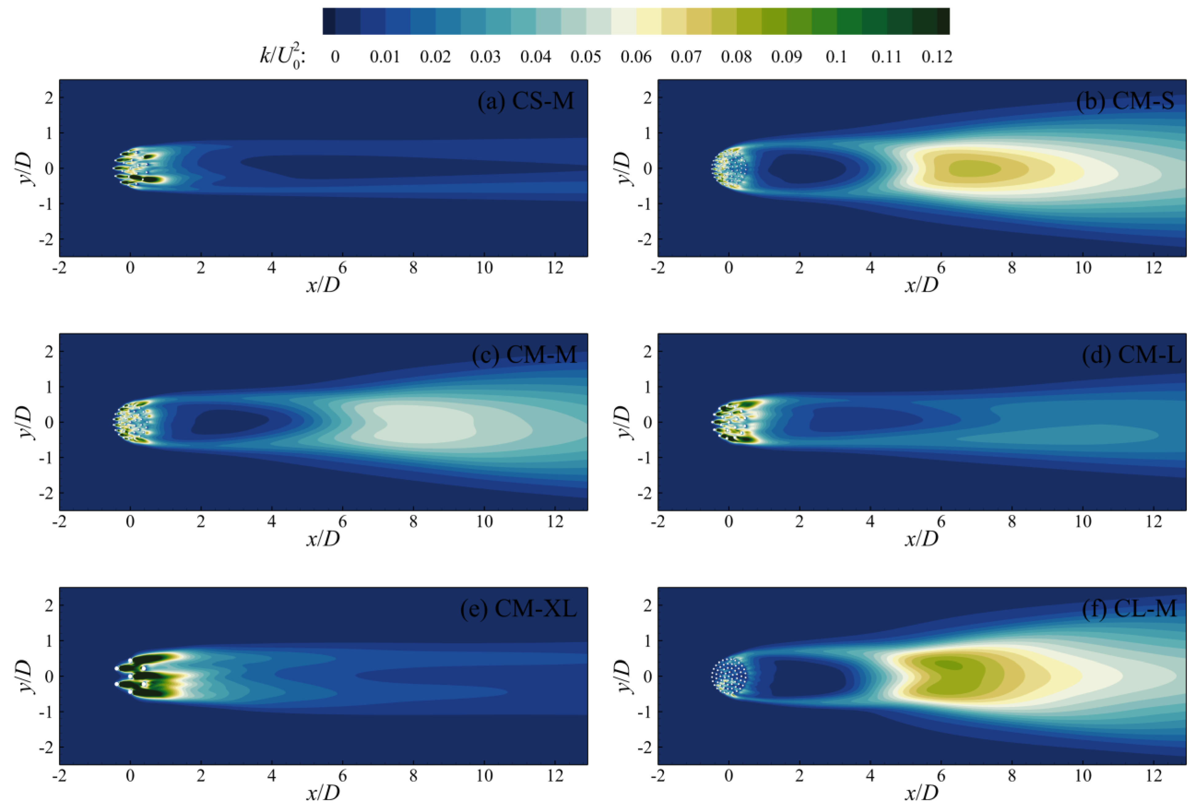
The turbulent kinetic energy within the cylinder array and its near-wake region mainly originates from element-scale wake vortices, while the high turbulence in the far field is primarily due to the array-scale transverse shear layers. As shown in Figure 7, in the CS-M case, due to the small transverse velocity gradient, only the interior of the array is covered by high turbulent kinetic energy, and the turbulent kinetic energy in the transverse shear layers dissipates rapidly along the longitudinal direction. However, in the denser CM-M and CL-M cases, the far-wake region exhibits significantly increased turbulent kinetic energy, caused by the intersection of the array-scale transverse shear layers at the wake centerline. For the same vegetation density, the distribution of far-field turbulent kinetic energy is generally influenced by d/D. As mentioned earlier, an increase in d/D reduces the transverse velocity gradient, leading to a predictable decrease in turbulent kinetic energy within the shear layers, as shown in Figure 7b,d. On the other hand, the stronger longitudinal outflow induced by the increase in d/D inhibits the formation and intersection of the transverse shear layers, resulting in the absence of high turbulent kinetic energy regions in the far field in the CM-XL case, and even preventing the formation of array-scale transverse shear layers. However, the high turbulent kinetic energy generated within the array extends a considerable distance into the wake region. The center of the high turbulent kinetic energy region shifts further downstream with increasing d/D; for instance, in the CM-S case, the center is approximately located at x ≈ 7D, while in the CM-M case, it is around x ≈ 8.5D, and in the CM-L case, it shifts even further downstream to x ≈ 10D. The changes in the distribution of turbulent kinetic energy induced by increasing d/D are equivalent to those resulting from decreasing vegetation density.

The turbulent kinetic energy distribution patterns shown in Figure 7 can be explained by the instantaneous vorticity depicted in Figure 8. Figure 8 presents the instantaneous vertical vorticity distribution for all simulated cases in this study, visualizing multi-scale wake vortices. As previously mentioned, when the group behavior of the cylinder elements is evident, array-scale transverse shear layers form at the shoulders of the array and grow wider downstream. Unlike the transverse shear layers of a solid cylinder of the same diameter, which immediately undergo Kármán vortex shedding at the downstream face of the cylinder, the transverse shear layers on the sides of the porous cylinder array are inhibited by the longitudinal outflow and only intersect and interact at a certain downstream distance. This causes the array-scale Kármán vortex street to occur further downstream. According to the 2D DNS results of Nicolle and Eames [19], all three vegetation densities included in this study should exhibit array-scale Kármán vortex streets. However, as shown by the instantaneous vorticity in Figure 8, this is not the case. The presence of array-scale Kármán vortices is influenced not only by the vegetation density λ but also by the relative diameter d/D. Specifically, when λ = 0.05, only the CS-S case with d/D = 0.036 produces alternating array-scale Kármán vortices. The CS-M and CS-L cases with larger d/D values exhibit only oscillations of the array-scale transverse shear layers accompanied by the shedding of smaller-scale vortices, with length scales significantly smaller than the array diameter. When the vegetation density increases to λ = 0.097, the CM-XL case with the largest d/D value does not generate significant array-scale transverse shear layers, resulting in a wake dominated by the merging of element-scale Kármán vortices. In contrast, the other three cases produce array-scale Kármán vortex streets, although their occurrence positions vary with respect to the array, shifting further downstream with increasing d/D. This explains the low turbulent kinetic energy in the far wake shown in Figure 7e and the decrease in turbulent kinetic energy in the far wake and transverse shear layer regions with increasing d/D, as shown in Figure 7b–e. When the vegetation density further increases to λ = 0.16, the longitudinal outflow is relatively weak, and array-scale Kármán vortex streets always appear. The distance between the occurrence position and the cylinder array once again shows a positive correlation with d/D.

When array-scale Kármán vortex streets form, a pair of counter-rotating Kármán vortices alternately shed downstream of the array with a fixed phase difference (1/2 shedding period T). When strong longitudinal outflow inhibits this, preventing the transverse shear layers on both sides of the array from intersecting, the shedding of shear layer vortices still occurs, characterized by the nearly simultaneous shedding of vortices from both shear layers with almost no phase difference. Additionally, array-scale Kármán vortex streets exhibit significant lateral oscillations, whereas the oscillations in the shear layer vortices are smaller in amplitude and remain in a parallel, non-intersecting state. When discussing array-scale Kármán vortex streets, it is arbitrary and inaccurate to judge their presence based solely on the vegetation density λ. This is because, even at a fixed λ value, the influence of the relative diameter d/D cannot be ignored, as shown in Figure 8. The vegetation density λ only reflects the proportion of bed area occupied by the cylinder elements and does not capture the variation within the array, such as the number and diameter of the cylinder elements. Besides λ, the non-dimensional frontal area aD (aD = 4λD/(πd) for circular cylinders) is also commonly used to characterize the density of the cylinder array. Unlike λ, the latter can reflect changes in d/D. When using aD as the independent variable, within the parameter range covered in this study, it can be concluded that array-scale Kármán vortex streets appear when aD ≥ 1.4. However, due to the low parameter resolution in the current study, aD = 1.4 is not an exact threshold for the occurrence of array-scale Kármán vortex streets. Further detailed parameter studies should be conducted to determine the precise aD threshold for the presence of array-scale Kármán vortex streets. It is expected that this threshold will lie between 1.0 and 1.4.

The intensity of the bleeding flow within the array not only controls the dynamics of element-scale wake vortices but also directly governs the velocity within the steady wake region. To further quantify the impact of vegetation density λ and relative diameter d/D on lateral flow deflection and the intensity of the bleeding flow within the array, Figure 9 shows the variation in the flow rate Q_t through the cylinder array with λ and aD. The flow rate Q_t through the cylinder array is non-dimensionalized by the flow rate Q_D in the unobstructed channel section where the cylinder array is located. Overall, the flow rate through the cylinder array decreases with increasing vegetation density. For the same vegetation density, an increase in d/D results in a higher throughflow. When aD is used to characterize the variation in Q_t, all data points collapse onto a single curve, eliminating the scatter caused by changes in d/D. This indicates that aD is the key parameter controlling the hydrodynamics around the circular cylinder array.

3.2. Drag Coefficient

The changes in flow deflection with vegetation density can be explained by the variation in drag coefficient. Here, we define the array drag coefficient ${\overline{C}}_D$ and the average cylinder element drag coefficient ${\overline{C}}_d$. This study focuses on time-averaged drag, so the drag coefficients discussed here refer to time-averaged drag coefficients. The array drag coefficient ${\overline{C}}_D$ for the 2D cylinder array in this study is calculated as follows:

$${\overline{C}}_D={\displaystyle \frac{{\displaystyle \sum _{i=1}^N{\overline{F}}_d^i}}{0.5\rho D{U}_0^2}}$$

(5)

The average cylinder element drag coefficient ${\overline{C}}_d$ is calculated as follows:

$${\overline{C}}_d={\displaystyle \frac{\frac{1}{N}{\displaystyle \sum _{i=1}^N{\overline{F}}_d^i}}{0.5\rho d{U}_0^2}}$$

(6)

Figure 10 shows the dependence of the array drag coefficient ${\overline{C}}_D$ and the average cylinder element drag coefficient ${\overline{C}}_d$ on vegetation density λ. Consistent with most existing studies, ${\overline{C}}_D$ generally increases with increasing λ. The underlying mechanism has been elucidated in numerous previous numerical studies [12,15,19,36,39], attributed to the enhanced lateral bleeding flow with increasing λ, which expands the width of the array wake region, thereby increasing the pressure difference between the upstream and downstream sides of the array. When λ is fixed, ${\overline{C}}_D$ monotonically decreases with increasing d/D (specific values can be seen in Table 1). This trend can also be explained by the variation in array wake width. As shown in Figure 5b–e, an increase in d/D results in weaker lateral bleeding flow, leading to a narrower wake region. Additionally, the stronger longitudinal bleeding flow induced by increasing d/D promotes wake velocity recovery, further reducing the array drag. At λ = 0.16, the influence of d/D on ${\overline{C}}_D$ is less pronounced than at lower vegetation densities, particularly with very close ${\overline{C}}_D$ values between the CL-S and CL-M cases. This is because, in the CL-M case, the lateral bleeding flow is already very weak, and further reducing the d/D value has a very limited impact on the lateral flow intensity.

Increasing λ and decreasing d/D both lead to weaker bleeding flow intensity within the array (see Figure 9), so the average cylinder element drag coefficient ${\overline{C}}_d$ not only decreases with increasing λ but also with decreasing d/D. Similar to ${\overline{C}}_D$, the sensitivity of ${\overline{C}}_d$ to changes in d/D also diminishes with increasing vegetation density. The opposing dependencies of the drag coefficients on λ and d/D again indicate that increasing the d/D value is equivalent to decreasing the λ value.

Figure 11 depicts the variation in the array drag coefficient ${\overline{C}}_D$ and the average cylinder element drag coefficient ${\overline{C}}_d$ with the non-dimensional frontal area aD. The three-dimensional LES values from Chang and Constantinescu [12] and the 2D DNS values from Nicolle and Eames [19] are also included. It can be seen that, when aD is used as the independent variable, all data points once again collapse onto a single curve, eliminating the dependency of the drag coefficients on d/D. The current 2D-URANS values show good consistency with the previous vortex-resolving method simulations. ${\overline{C}}_D$ and ${\overline{C}}_d$ monotonically increase and decrease, respectively, with increasing aD, and they follow the empirical relationships ${\overline{C}}_D=0.34\ln \left(aD\right)+0.78$ and ${\overline{C}}_d=-0.42\ln \left(aD\right)+0.82$.

The good agreement between the 2D DNS values from Nicolle and Eames [19] and the current calculations at similar aD values indicates a weak dependency of the array drag coefficient on the array Reynolds number. The former exhibits an array Reynolds number Re_D = 2100 and the latter exhibits Re_D = 10000. The insensitivity of the array drag coefficient to the Reynolds number has also been observed by Taddei et al. [36]. Kazemi et al. [40] noted that this phenomenon occurs when Re_D > 1000.

3.3. Steady Wake Parameters

The longitudinal distribution of the time-averaged longitudinal velocity ū/U₀ and the turbulent kinetic energy k/U₀² along the array centerline is shown in Figure 12. The upstream inflow begins to decelerate significantly at a distance of approximately D from the array. Downstream of the array, the variation in longitudinal velocity undergoes three stages. The first stage is the steep drop in longitudinal bleeding flow velocity exiting the downstream face of the cylinder array, which then transitions to a slow decrease after reaching a certain value. This marks the beginning of the second stage, the steady wake region. The position where the longitudinal velocity decreases to its minimum corresponds to the end of the steady wake region. After this, the expansion of the transverse shear layers from both sides of the array toward the wake centerline entrains high longitudinal momentum into the wake region, promoting the recovery of wake velocity. The wake velocity begins to gradually increase until it recovers to a constant value, corresponding to the third stage. Vertical arrows in Figure 12a indicate the positions where the longitudinal velocity decreases to its minimum. For cylinder arrays with high λ values, the position of the minimum wake velocity is closer to the cylinder array. For cylinder arrays with the same λ value, increasing d/D causes the position of the minimum longitudinal velocity to move downstream. High vegetation density and small relative array diameter both contribute to a faster recovery of wake velocity.

The turbulent kinetic energy rapidly decays downstream of the array, maintaining a relatively low turbulence level within the steady wake region. This is a typical characteristic of the steady wake region. At the downstream end of the steady wake region, the interaction of the array-scale transverse shear layers originating from the shoulders of the cylinder array significantly increases the turbulent kinetic energy, causing a distinct peak. The magnitude of the turbulent kinetic energy peak is negatively correlated with d/D at a fixed λ value, and positively correlated with λ at a fixed d/D value.

The bleeding velocity U_e exiting the array from the trailing edge is a key parameter controlling the characteristics of the wake. Following Taddei et al. [36], U_e is defined as the average longitudinal velocity at x = 0.52D. Figure 13a shows the variation in the non-dimensional bleeding outflow velocity U_e/U₀ with aD for all computational cases. All data points once again collapse onto a single curve. U_e/U₀ monotonically decreases with increasing aD, following the empirical relationship $U_e/U_0=-0.32\ln \left(aD\right)+0.59$. The velocity within the steady wake region is typically characterized by U₁, the value wherein the longitudinal velocity along the array centerline transitions from a steep to a gradual decline [12,13]. The length of the steady wake region, L₁, is defined as the longitudinal distance from the position where the velocity decreases to its minimum to the downstream edge of the cylinder array. Figure 13b,c, respectively, show the variations in U₁/U₀ and L₁/D with aD. Results from Chang and Constantinescu [12] are also included. The longitudinal velocity contour plots in Figure 4 already indicate that the steady wake region velocity decreases with increasing λ and increases with increasing d/D. However, when the effects of λ and d/D are combined into the non-dimensional parameter aD, U₁ shows a clear monotonic decrease with increasing aD and collapses onto a single curve $U_1/U_0=-0.41\ln \left(aD\right)+0.54$. The length L₁ of the steady wake region shows some scatter but generally exhibits a negative correlation with aD.

4. Conclusions

This study conducted a 2D-URANS investigation of the flow and turbulent structures as well as the drag characteristics within and downstream of emergent vegetation patches. The emergent vegetation patch is generalized as a two-dimensional circular cylinder array arranged in concentric rings, which is a reasonable approximation for areas where emergent vegetation is distant from the bed surface. The simulations kept the diameter of the cylinder array constant while varying the number of elements and their diameter within the array to create different vegetation density λ values and relative diameters d/D to explore their effects on wake patterns and drag forces.

Increasing d/D and decreasing λ are equivalent in that both contribute to increasing the spacing between elements within the array, allowing for the formation and development of stem-scale Kármán vortices. For a fixed vegetation density, decreasing d/D leads to stronger lateral flow deflection and weaker throughflow, resulting in stronger transverse shear layers of the array. It is arbitrary and inaccurate to predict the presence of array-scale Kármán vortex streets solely based on λ. This is because, even at a fixed λ value, the impact of d/D on the longitudinal outflow intensity and transverse shear layers directly determines the formation of Kármán vortex streets. Using the non-dimensional frontal area aD, which comprehensively characterizes vegetation density and cylinder element diameter changes, is a better choice. Within the parameter range covered in this study, array-scale Kármán vortex streets appear when aD ≥ 1.4.

The drag characteristics of the cylinder array were quantified using the array drag coefficient ${\overline{C}}_D$ and the average element drag coefficient ${\overline{C}}_d$. For a fixed d/D value, ${\overline{C}}_D$ increases with increasing λ, while ${\overline{C}}_d$ decreases. For the same vegetation density, increasing d/D results in a decrease in ${\overline{C}}_D$ and an increase in ${\overline{C}}_d$, and the sensitivity of both to changes in d/D decreases with increasing λ. When parameterizing the drag coefficients using aD, all data points from this study and previous studies collapse onto a single curve, following the relationships ${\overline{C}}_D=0.34\ln \left(aD\right)+0.78$ and ${\overline{C}}_d=-0.42\ln \left(aD\right)+0.82$.

The flow through the cylinder array is influenced by both vegetation density λ and relative diameter d/D, resulting in a monotonic relationship between longitudinal outflow velocity U_e and aD. Due to the longitudinal outflow, the length of the steady wake region L₁ decreases with increasing aD, but shows some data scatter.

The findings of this study provide valuable insights into the hydrodynamic characteristics and drag forces of circular cylinder arrays with varying vegetation densities and relative diameters. The non-dimensional frontal area (aD) has been identified as a crucial parameter for predicting the presence of array-scale Kármán vortex streets, offering an effective control parameter for sediment transport calculations. These results have significant implications for the design and management of vegetated water bodies, such as wetlands, riverine systems, and coastal areas, where controlling sediment dynamics and ensuring the stability of vegetation patches are critical. Furthermore, this research can guide future studies in optimizing vegetation arrangements to enhance ecological functions and resilience in aquatic environments.