the Creative Commons Attribution 4.0 License.
the Creative Commons Attribution 4.0 License.
A global lake and reservoir volume analysis using a surface water dataset and satellite altimetry
Tim Busker
Ad de Roo
Emiliano Gelati
Christian Schwatke
Marko Adamovic
Berny Bisselink
Jean-Francois Pekel
Andrew Cottam
Lakes and reservoirs are crucial elements of the hydrological and biochemical cycle and are a valuable resource for hydropower, domestic and industrial water use, and irrigation. Although their monitoring is crucial in times of increased pressure on water resources by both climate change and human interventions, publically available datasets of lake and reservoir levels and volumes are scarce. Within this study, a time series of variation in lake and reservoir volume between 1984 and 2015 were analysed for 137 lakes over all continents by combining the JRC Global Surface Water (GSW) dataset and the satellite altimetry database DAHITI. The GSW dataset is a highly accurate surface water dataset at 30 m resolution compromising the whole L1T Landsat 5, 7 and 8 archive, which allowed for detailed lake area calculations globally over a very long time period using Google Earth Engine. Therefore, the estimates in water volume fluctuations using the GSW dataset are expected to improve compared to current techniques as they are not constrained by complex and computationally intensive classification procedures. Lake areas and water levels were combined in a regression to derive the hypsometry relationship (dh ∕ dA) for all lakes. Nearly all lakes showed a linear regression, and 42 % of the lakes showed a strong linear relationship with a R2 > 0.8, an average R2 of 0.91 and a standard deviation of 0.05. For these lakes and for lakes with a nearly constant lake area (coefficient of variation < 0.008), volume variations were calculated. Lakes with a poor linear relationship were not considered. Reasons for low R2 values were found to be (1) a nearly constant lake area, (2) winter ice coverage and (3) a predominant lack of data within the GSW dataset for those lakes. Lake volume estimates were validated for 18 lakes in the US, Spain, Australia and Africa using in situ volume time series, and gave an excellent Pearson correlation coefficient of on average 0.97 with a standard deviation of 0.041, and a normalized RMSE of 7.42 %. These results show a high potential for measuring lake volume dynamics using a pre-classified GSW dataset, which easily allows the method to be scaled up to an extensive global volumetric dataset. This dataset will not only provide a historical lake and reservoir volume variation record, but will also help to improve our understanding of the behaviour of lakes and reservoirs and their representation in (large-scale) hydrological models.
- Article
(6674 KB) - Full-text XML
-
Supplement
(185 KB) - BibTeX
- EndNote
Reservoirs and lakes cover a small part of the Earth's land surface (∼3.7 %, Verpoorter et al., 2014), but are crucial elements in the hydrological and biochemical water cycles. Reservoirs have been constructed at a rapid pace between the 1950s and 1980s, and the construction of new reservoirs will continue over the coming century (Chao et al., 2008; Duan and Bastiaanssen, 2013). Reservoirs therefore have an increasing impact on river discharges, as they are able to alter the hydrograph by storing, retaining and releasing water. They are a valuable resource for hydropower, domestic and industrial water use, wetlands, and are the primary water resource for nearly half of the irrigation-based agricultural sector by supplying approximately 460 km3 of water per year (Biemans et al., 2011; Hanasaki et al., 2006). Moreover, they play a crucial role in biogeochemical activity by emitting vast amounts of CO2, triggered by CO2 saturation in lakes and wetlands worldwide (Balmer and Downing, 2011; Cole et al., 2007; Frey and Smith, 2005; Richey et al., 2002).
The amount of water in a reservoir results from the balance of inflow (i.e. direct precipitation, inflowing river discharge, discharge from riparian communities and industries, and subsurface inflow) and outflow (i.e. direct evaporation, withdrawals, reservoir outflow and groundwater percolation) (Duan and Bastiaanssen, 2013). A long-term imbalance can result in considerable reductions in water storage, as frequently observed around the globe in, for example, Lake Mead, Lake Powell, Lake Poopo and the Aral Sea (Barnett and Pierce, 2008; Micklin, 2016). Reduced water availability in the reservoirs may then result in reductions in hydropower energy production and/or irrigation water availability and lead to economic and societal damage. Many studies have already pointed out that population and economic growth, together with climate change and increasing energy and food requirements, will put increasing pressure on water resources (Haddeland et al., 2014; Liu, 2016). A proper understanding of the historical dynamics of reservoirs as a source of water for irrigation, drinking water and energy production, as well as a buffer for flood protection, is also essential to improve the quality of future projections on global water resources.
While for individual river basin studies information on reservoirs may be available, especially for larger scale water resource studies at national, continental and global scale, almost no historical records on reservoirs are readily available to run, calibrate and validate hydrological models (Hanasaki et al., 2006). Moreover, in situ lake level and volume measurements are sparse – especially in developing countries – and have even decreased around the globe during recent years (Duan and Bastiaanssen, 2013). Even if water levels or volumes are monitored, the information is rarely freely available due to strategic political, commercial or national legislation reasons. Therefore, only a few comprehensive global lake and reservoir datasets exist (e.g. Downing et al., 2006; Lehner and Döll, 2004; Meybeck, 1995; Verpoorter et al., 2014) and if they provide a water storage estimation, these estimates are not dynamic or do not provide data over a longer time series. Therefore, remotely sensed data may be a valuable alternative to monitor water volumes in lakes and reservoirs over the last few decades.
Monitoring lakes and reservoirs using remote sensing has gained much attention over the last few years (e.g. Avisse et al., 2017; Crétaux et al., 2016; Duan and Bastiaanssen, 2013; Frappart et al., 2006b; Gao et al., 2012; Smith and Pavelsky, 2009). Most of these publications focussed on volume variations by combining altimetry water level with lake area from a multispectral sensor. Landsat or MODIS imagery is commonly used to estimate water surface areas, by classifying the satellite images capturing the water body. The classification procedure is demanding and computationally intensive if large areas or many images are classified, and misclassifications may occur because of the diversity of spectral signatures emitted by water surfaces. Therefore, calculating lake areas is often a constraining factor in lake volume calculations. They are predominantly used for the lake hypsometry relationship (dh ∕ dA), but they normally do not provide any temporal details and therefore cannot be used to calculate volume variations on their own (e.g. Duan and Bastiaanssen, 2013; Ran and Lu, 2012; Zhang et al., 2006). Where lakes areas have been calculated to any great extent, this has only been done for a couple of lakes or at a lower resolution (e.g. Smith and Pavelsky, 2009; Tong et al., 2016). Thus, measuring lake volume variations from space is commonly a trade-off between the number of lakes analysed, the resolution of the lake area calculation and the number of historical lake areas that can be calculated. In this study however, by using the pre-processed recently available Joint Research Centre (JRC) Global Surface Water (GSW) dataset with a high temporal and spatial resolution and extensive validation, this trade-off is no longer an issue. Here we perform volume variation estimations globally with a 30 m resolution from 1984 onwards, using all Landsat images available after the launch of Landsat 5. Thereby this study aims to improve on current monitoring techniques and to develop an automatic methodology that is relatively easy to implement at a large scale.
The paper is organized as follows. Section 2 presents the data used in this research, providing a description of the DAHITI altimetry database and an overview of the GSW dataset. Section 3 contains a description of the methods applied, while Sect. 4 gives a description of the results. Section 5 presents a discussion, and finally the conclusions and recommendations are presented in Sect. 6.
2.1 Satellite altimetry
Satellite altimetry was initially designed for observing the ocean's surface. But for more than 10 years now, satellite altimetry has proven to be a suitable tool for measuring water heights of lakes and rivers. Numerous studies have already shown the potential of estimating water level time series over inland waters using different altimeter missions such as TOPEX/Poseidon (Birkett, 1995), Envisat (Frappart et al., 2006a), Saral (Schwatke et al., 2015b), Cryosat-2 (Villadsen et al., 2015) or ICESat (Zhang et al., 2011). Water levels from satellite altimetry have also been used for hydrological applications such as the estimation of river discharge (Kouraev et al., 2004; Tourian et al., 2017; Zakharova et al., 2006) and lake volumes (Duan and Bastiaanssen, 2013; Tong et al., 2016; Zhou et al., 2016).
Satellite altimetry has the potential to provide reliable water level time series of globally distributed inland water bodies over the last 20 years. TOPEX/Poseidon and Jason-1/-2/-3 have an identical orbit configuration with a 9.9156-day repeat cycle and a track separation of about 300 km at the Equator. ERS-1/-2, Envisat and SARAL flew on an orbit with a 35-day repeat cycle and a track separation of about 80 km at the Equator. The combination of different altimeter missions is essential to increase the temporal resolution, spatial resolution and length of the water level time series. In order to combine altimeter data from different missions, a mission-dependent range bias resulting from a multi-mission crossover analysis has to be taken into account to achieve long-term homogenous water level time series (Bosch et al., 2014).
The estimation of water level time series for small lakes, reservoirs or rivers is very challenging. Due to coarse mission-dependent ground tracks with a cross-track spacing of a few hundred kilometres, larger lakes and reservoirs have a much higher probability to be crossed by a satellite track than smaller ones. Moreover, small water bodies tend to have a relatively big altimeter footprint compared to their size, which will affect the resulting shape of the returning waveform. The diameter of the footprint is mainly influenced by the water roughness (i.e. surface waves) and surrounding topography. In reality, the diameter of the footprint can therefore vary between 2 km over the ocean and up to 16 km for small lakes with considerable surrounding terrain topography (Fu and Cazenave, 2001). These land influences and surface waves within the altimeter footprint can affect the altimeter waveforms and require an additional retracking to achieve more accurate ranges. In order to achieve accurate results for small water bodies, the conditions have to be ideal, meaning a low surrounding topography, low surface waves, and perpendicular crossings of the altimeter track and water bodies' shores. In these ideal cases, satellite altimetry has the capability to observe rivers with a width of about 100–200 m or lakes with a diameter of a few hundred metres. The off-nadir effect is another problem which can occur when investigating smaller water bodies. In general, satellite altimetry measures in the nadir direction, but if the investigated water body is not located in the centre of the footprint, then the radar pulses are not reflected in the nadir direction, which leads to longer corrupted ranges that must be taken into account (Boergens et al., 2016).
In this paper we use water level time series from the “Database for Hydrological Time Series over Inland Waters” (DAHITI) as input data for the volume estimation. DAHITI is an altimetry database launched in 2013 by the “Deutsches Geodätisches Forschungsinstitut der Technischen Universität München” (DGFI-TUM). The data are accessible through a user-friendly web service (http://dahiti.dgfi.tum.de/en/, last access: 14 July 2018) and currently include water levels for more than 780 lakes, reservoirs, rivers and wetlands. The processing strategy of DAHITI is based on a Kalman filtering approach and an extended outlier detection (Schwatke et al., 2015a) which combines different altimeter missions such as TOPEX/Poseidon, Jason-1, 2 and 3, GFO, Envisat, ERS-1 and 2, Cryosat-2, and SARAL/AltiKa. DAHITI uses only high-frequency altimeter data. Depending on the measurement frequency of the altimeter, heights are measured every ∼620 (10 Hz), ∼374 (20 Hz), ∼294 (18 Hz) or ∼173 m (40 Hz) along the altimeter track. To achieve more accurate ranges over inland waters, the Improved Threshold Retracker (Hwang et al., 2006) is used for the reanalysis of the altimeter measurements. The DAHITI approach provides all water level time series error information based on formal errors of the Kalman filtering.
The quality of the water level time series from satellite altimetry in DAHITI has been validated with in situ data and varies depending on the extent of the inland water body and length of the crossing altimeter track. For large lakes with ocean-like conditions (such as the Great Lakes), accurate measurements can potentially be achieved with a root-mean-square error (RMSE) as low as 4–5 cm, while for smaller lakes and rivers the RMSE could increase to several decimetres (Schwatke et al., 2015a). However, no clear relationship was observed between lake size and altimetry accuracy, as the quality of water level time series is not only dependent on the target size, but also on many other factors (e.g. surrounding topography, surface waves, winter ice coverage, the position of altimeter track crossings).
2.2 The JRC Global Surface Water (GSW) dataset
The JRC GSW dataset (Pekel et al., 2016) maps the temporal and spatial dynamics of global surface water over a 32-year period (from 16 March 1984 to 10 October 2015) at 30 m resolution. This dataset was produced by analysing the whole L1T Landsat 5, 7 and 8 archive. At the time of the study, it represented 3 066 080 images (1823 terabytes of data) and covered 99.95 % of the landmass. The analysis was performed thanks to a dedicated expert system classifier. The inference engine of the classifier is a procedural sequential decision tree, which used both the multispectral and multitemporal attributes of the Landsat archive as well as ancillary data layers. It assigned – in a consistent way in both space and time – each pixel to one of three target classes, either water, land or non-valid observations (snow, ice, cloud or sensor-related issues). Classification performance, measured using over 40 000 reference points, revealed the high accuracy of the classifier: less than 1 % of false water detections, and less than 5 % of omission (Pekel et al., 2016). Thanks to its technical characteristics, the GSW dataset constitutes a very valuable long-term surface water record.
The stack of classified images constitutes the long-term water history documenting the “when and where” of the water presence. This information is recorded in the monthly water historical dataset – a set of 380 global-scale maps documenting the water presence for each month of the 32-year archive. This monthly information constitutes the most comprehensive and detailed dataset of the GSW. Eight additional information layers, documenting different facets of the surface water dynamics, are also available within the GSW dataset: (1) water occurrence, (2) occurrence change intensity, (3) seasonality, (4) recurrence, (5) transitions, (6) maximum water extent, (7) monthly recurrence and (8) yearly history. In the framework of this study, the monthly water history and maximum water extent (MWE) – a map documenting places where water has been detected at least once over the 32 years were used.
The GSW dataset was completely developed using Google Earth Engine and all of the layers are available through the Earth Engine catalog (Gorelick et al., 2017). Moreover, Earth Engine is used in this research to calculate the monthly lake area time series. Earth Engine is a cloud-based global-scale platform optimized for parallel geospatial analyses and data management in Earth sciences, using Google's computational power (Gorelick et al., 2017). Earth Engine allowed the analysis of lakes at global scale in high detail, while maintaining a high resolution of 30 m.
3.1 Calculating monthly lake areas
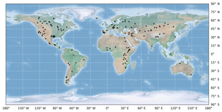
Monthly time series of lake areas have been calculated for 137 lakes over all continents (Fig. 1). These contained nearly all lakes available in the DAHITI altimetry database at the time of processing. No additional criteria were set for this study, as the GSW dataset covers all lakes globally. For 380 months over the period 1984–2015 lake areas were calculated using a dedicated Google Earth Engine script. For each lake, a region of interest (ROI) was set by a manually drawn polygon that was approximately equal to the MWE of the lake (Fig. 2). For every month, lake areas were calculated directly from the GSW monthly historical dataset, by counting the number of water pixels inside the polygon and multiplying this by the pixel area. To improve the accuracy of the area calculations, the amount of non-valid observations (no-data pixels) within the MWE, compared to all MWE pixels within the ROI, has been expressed as the no-data fraction. This no-data fraction has been used to filter accurate and less accurate area observations in the regression analysis and volume calculations (see Sect. 3.2). The white striping observed for Lake Mead in Fig. 2 is an example of a lack of data that is caused by Landsat sensor issues.
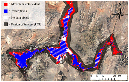
Figure 2An example of the area input data for Lake Mead (US) for February 2015, where the maximum water extent is marked as red, water as blue and a lack of data as white pixels.
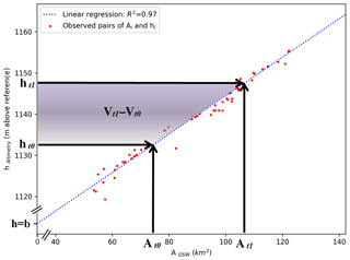
Figure 3Volume variation calculation for Lake Eucumbene (Australia). The observed monthly pairs of A and h (red dots) are used to estimate a linear regression (blue dashed line) that is used to calculate volumetric changes. The volumetric change from t0 to t1 is equal to the purple area and can be visually interpreted as a 2-D lake section.
3.2 Calculating lake volumes variations
The volume of a lake or reservoir is a function of the water area (A) and level (h), derived from the hypsometry relationship (dh ∕ dA). Monthly lake areas were only used in the regression if the no-data percentage was below 1 %, because only accurate areas were desired to construct the regression line. As exact dates are not provided by the GSW dataset, the altimetry data were first averaged per month, after which monthly water levels (hAltimetry) were coupled with monthly area values (AGSW). These are illustrated with red dots in Fig. 3 for Lake Eucumbene (Australia). The water-level–area pairs were assumed to give linear hypsometric relationships of the water bodies (Fig. 3, dashed blue line):
where Ai and hi are the area and water level respectively, a and b are the slope and intercept parameters, and εi is the error term or residual for time step i. The parameters a and b have been derived by minimizing the residual sum of squares (RSS, i.e. ), using an ordinary least squares regression (OLS) technique. Therefore, the resulting residuals are uncorrelated and zero-mean normally distributed random variables with variance σ2: ). The hypsometric relations can be integrated to obtain the expected volume of the water body:
where Ai is the monthly calculated lake area derived from the GSW dataset, hi is the water level from altimetry and b is the water level of the theoretical lake bottom from the linear regression at A=0, for time step i. By substituting the regression equation in Eq. (2), the expected value of the water volume can be calculated using h or A only:
Using these equations, absolute volumes are computed by using only the area or water level estimates, giving two different volumetric time series: VGSW and Valtimetry. Rather than a 1 % no-data threshold in the regression analysis for lake area estimations, a 5 % no-data threshold has been applied to area estimations used for the volume calculation. This resulted in the best trade-off between the number of observations from the GSW dataset and the accuracy of the estimates. The extrapolated part of the regression line, and therefore in particular the theoretical lake bottom b, should be considered with caution, as the hypsometry relationship may change outside the observational range. The absolute volumes from Eq. (3) are therefore converted to volume variations from t0 to ti (Fig. 3, purple area). Most estimated volume variations were calculated using h or A values inside the observed part of the regression line (i.e. inside the range of observed h–A pairs). However, some volumes were estimated with A or h values that are outside such a range. These volume estimates use an extrapolated lake hypsometry which is not observed and therefore more uncertain. These estimates are therefore separately classified in the volumetric plots.
A 95 % prediction interval (PI) and confidence interval (CI) have been calculated around the linear regression line using Eqs. (S13) and (S14), taking into account the slope and intercept parameter uncertainty and the standard deviation of the residuals. The PI around the linear regression has been propagated to a PI around the estimated volume variations of VGSW: , where and V0 is a reference volume. This PI is based on the variance of the volume difference estimation , as given by Eq. (S18). The derivation of is provided in the Supplement.
Not all lakes showed considerable area fluctuation, as some lakes and reservoirs are artificially bounded or have very steep banks. The coefficient of variation (CV) has been calculated from the area observations to express lake area variation normalized by mean lake size. The signal-to-noise ratio (SNR) for lakes with a very small CV is likely to be low as errors due to a lack of data, misclassifications and the lake border discretization with 30 m pixels will mask the actual area variations. A linear regression between variable lake levels and nearly constant lake areas would thus not be feasible. Therefore, the areas of lakes with a very small CV were interpreted to be constant. Lake volumes were still calculated, but only by multiplying the mean area with water level variations as observed by altimetry.
3.3 Validation of the volume estimates
The validation has been carried out using the Pearson correlation coefficient r, the RMSE and the normalized RMSE (NRMSE). The Pearson correlation coefficient r measures the linearity between in situ and estimated volume variations, while the RMSE accounts for the absolute error. The NRMSE has been calculated by normalizing the RMSE with the range of in situ lake volume variations:
where Obsmax and Obsmin are the maximum and minimum observed in situ volumes since 1984.
4.1 Regression analysis
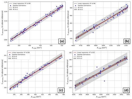
A total of 137 lakes and reservoirs have been analysed over all continents. The linear OLS regression analysis resulted in highly variable R2 values among the lakes and reservoirs. Low R2 values were observed to be caused mainly by noise rather than non-linear hypsometry, as only four lakes (Tawakoni, Urmia, Tsimlyansk and Eagle) returned a clear non-linear hypsometry relationship (see Discussion). The mean R2 of all 137 lakes is only 0.58, but 58 lakes showed a R2 > 0.8 with an average of 0.91. Lake Eucumbene (Australia), Lake Kariba (Zambia), Lake Powell, Lake Mead and Hubbard Creek Reservoir (US) are examples of these lakes, with high R2 values and low regression residuals. The regression results for Lake Powell, Kariba, Mead and Nasser are shown in Fig. 4, with R2 values of 0.99, 0.96, 0.98 and 0.92 respectively. Two considerable outliers are present in the linear regression of Lake Nasser (Fig. 4d). They have a considerable effect on the width of the CI and PI, as these uncertainty bounds decreased by almost a factor of 2 (47 % and 49 %, respectively) when they were removed. A discussion on the causation of these outliers is given in Sect. 5.3.
4.2 Division of the lakes in groups
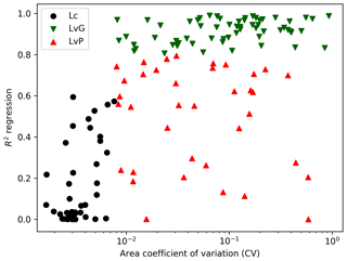
Based on the R2 values from the regression and the area CV, the lakes have been subdivided into lakes with a constant area (Lc; CV < 0.008), lakes with a variable area (Lv; CV > 0.008) where the latter (Lv) category has been further subdivided into lakes with a good performance (LvG; R2 > 0.8) and lakes with a poor performance (LvP; R2 < 0.8) (Fig. 5). A total of 42 lakes with a CV < 0.008 are categorized as Lc, as all these lakes returned a R2 < 0.6 with an average of 0.16 (black circles, Fig. 5). As explained in the last paragraph of Sect. 3.2, these lakes have a very small variation in area, resulting in a low SNR and consequently in regressions with large residuals. Therefore, these lakes were assumed to have a constant area and their volume was calculated by multiplying water level observations with the average of the GSW lake area estimates. For lakes in the Lv category (CV > 0.008), considerable monthly area variations were observed and the regressions returned mostly acceptable R2 values with an average of 0.76. A total of 58 lakes in this category were classified in sub-category LvG as they showed a R2 > 0.8, with an average of 0.91 (green triangles, Fig. 5). For these lakes, volumes have been calculated using linear regressions. For 37 lakes with a variable area, the residuals were higher, resulting in a R2 < 0.8 and a mean of 0.50 and therefore they are classified in sub-category LvP (red triangles, Fig. 5). Volume variations were not calculated for these lakes. The R2 threshold has been set to 0.8 as three out of five lakes in the R2 range of 0.75–0.8 (Tsimlyansk Reservoir, Lake Eagle and Lake Tawakoni) showed clear non-linear area–level relationships, while all lakes with R2 > 0.8 showed approximately linear area–level relationships. Therefore, the volume variations of lakes with a R2 > 0.8 are well represented by our linear regression-based volume calculation method. A table for each of the above-mentioned categories, showing the most important lake properties and the R2 values, is given in Appendix A1.
4.3 Volumetric results
For a total of 100 lakes (58 lakes with variable area and 42 lakes with constant area), the volume variation time series have been calculated, using both water levels (VAltimetry) and water areas (VGSW) as inputs. Volumetric results of the variable-area lakes (LvG) Powell, Kariba, Mead and Nasser are outlined below and are shown in Fig. 6. VAltimetry or VGSW estimates inside the observational range of the regression (h–A pairs) are coloured blue and red. Some volume estimates are derived from observations outside the regression range; these are extrapolated estimates and are displayed with a darker colour tint. The red line displays the best estimate of the volume variation as calculated with observed water classifications in the GSW dataset (i.e. total area of surface water). The red shaded area displays the upper volume boundary on the VGSW estimates, as derived from the GSW dataset pixels classified as no data within the MWE (max 5 %; see Sect. 3.2). These no-data pixels could theoretically be covered with water for that month, and this would increase the estimated volume. In this case the volume variation estimate would be somewhere within the red shaded area. The upper limit of the red shaded area would thus be reached if all no-data pixels within the MWE contain surface water during that particular month. Another source of uncertainty is the uncertainty of the regression parameters, which is represented by the grey shaded area. It shows the effect of the 95 % PI on the volume variation estimates as calculated with Eq. (S18). Note that both uncertainty indicators (red and grey shaded area in Fig. 6) are point estimators of the uncertainty at the VGSW estimates, which are linearly connected to increase the readability of the plot. Therefore, caution should be used when interpreting the uncertainty in the gaps between the observed data points (e.g. between 1987 and 1998 in Fig. 6d).
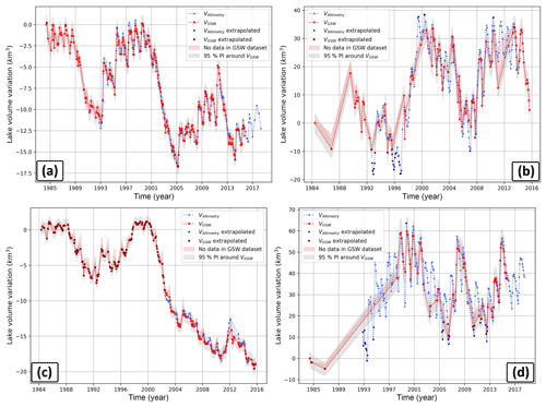
Figure 6Lake volume variations for Lake Powell (a), Kariba (b), Mead (c) and Nasser (d) using VAltimetry (blue) and VGSW (red).
Figure 7 summarizes the volumetric results, by showing lake location, lake type (Lc, LvG or LvP) and the average volumetric change. The volumetric change shows the magnitude of reduction (red circles) or increase (blue circles) in average water storage between the periods 1984–2000 and 2000–2015 for LvG, and from 2000–2008 to 2008–2016 for Lc. Slightly more lakes showed a positive change (60) than a negative one (40). Considerable reductions of water storage were observed in the western US, due to major average volume declines in Lake Mead (11 km3), Powell (6 km3) and the Great Salt Lake (16 km3). Average increases were found for the Great Lakes and most of the analysed lakes in southeastern Africa. A clear spatial pattern between Lc and Lv is observed in North America. An abundance of Lc water bodies were located above 42∘ N (64 %, primarily in Canada), while water bodies between 42 and 15∘ N (in the US and Mexico) were only classified as Lv. This spatial difference in lake extent variation is potentially caused by a combination of different climate characteristics (precipitation and evaporation), human regulations, and topography between Canada and US–Mexico. Furthermore, the US has a high proportion of LvG classifications compared to LvP (especially the western US), mainly due to the relatively high number of historical Landsat images from 1984 and their high quality (see Sect. 5.2). Changing the R2 threshold from 0.8 to 0.6 did not considerably change the global spatial distribution of LvP classifications. The spatial distribution of water bodies with extremely low R2 values (R2 < 0.3) was uniform over the whole globe.
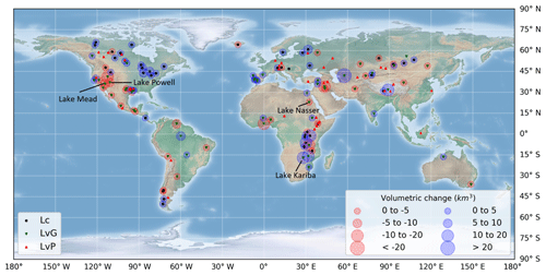
Figure 7Lake and reservoir types (constant area (Lc), variable area with good (LvG) and poor (LvP) regression performance) with the average volume changes.
Lake Mead was formed after the construction of the Hoover Dam during the 1930s, in the former steep V-shaped slopes created by the Colorado River. It is located approximately 50 km east of Las Vegas in the Black Canyon, Arizona–Nevada (Fig. 7). With a maximum depth of 158 m and a maximum capacity of 33–35 km3, Lake Mead is the largest reservoir in the US by capacity and the second largest (after Lake Powell) by water area (Barnett and Pierce, 2008; Holdren and Turner, 2010). The lake showed a considerable reduction in water storage between 1984 and 2015 (Fig. 6c). Between two periods of maximal reported capacity (1984–1988 and 1998–2000), a small decrease in capacity of around 7 km3 was observed. From its historical maximum capacity in 2000, the water level dropped 40 m between 2000 and 2010 (Cook et al., 2007; Duan and Bastiaanssen, 2013), mainly because of a combination of water abstractions by around 25 million people and multiple intensive droughts (Holdren and Turner, 2010). This reduction in water storage is also reported by the satellite estimates. According to our estimates, Lake Mead lost approximately 20 km3 of water from 2000 to 2015 (Figs. 6c, 7). Using the USGS in situ measurement of storage volume of 31 km3 in 2000; this is an almost 70 % reduction in water storage over the last 15 years.
Lake Nasser is a crucial resource for Egypt's population, functioning as a source for irrigational water and electricity and as an important flood-control mechanism. With an estimated maximum storage capacity of 162 km3, Nasser is the main freshwater resource for approximately 85 % of the Egyptian population (Gao et al., 2012; Muala et al., 2014). The lake shows a strong annual cycle, with declines in water storage during the first half of the year and increases during the second half of the year (Fig. 6d). The annual cycle amplitude varies from around 10 to 20 km3. Besides this yearly fluctuation, Lake Nasser features an even longer inter-annual variability. From the lowest recorded volume over 1985–1993, water storage increased at least 40 km3 to record-high estimates in the period 1998–2002. From 2002, the lake shows a decreasing trend towards 2006, during which time it lost approximately 30 km3. Two peaks were observed over 2007–2009 and in 2005, when the lake gained 30–35 km3 of water and subsequently lost the same amount. The lake showed an average volume decrease over the whole observational period of only 1.8 km3, which is negligible compared to the size of the lake (Fig. 7).
Lake Kariba formed after the construction of the Kariba Dam on the Zambezi River on the border of Zimbabwe and Zambia (Berg et al., 1996). It has an average surface area of 5364 km2 and with an estimated capacity of 185 km3 it is the largest reservoir in Africa by volume (LakeNet, 2003). The reservoir shows a consistent seasonal variation, with increases of around 10–20 km3 during the first 5 months, and decreases over the last 7 months of the year (Fig. 6b). Moreover, the lake gained at least 45 km3 of water from 1996 to 1999. From 2000 to 2007, the volume decreased again by approximately 30 km3. From 2008, the water volume increased to a maximum reported capacity in May 2010. From July 2014, the lake shows a constantly decreasing trend towards the last year of the data (September 2015). Over the whole observational period, the average storage of the lake increased by 15 km3 (Fig. 7).
With an area of 653 km2, Lake Powell is the largest lake in the US by water surface area (Barnett and Pierce, 2008; Benenati et al., 2000). Its maximum capacity of 33.3 km3 is slightly less than that of Lake Mead (Benenati et al., 2000; Holdren and Turner, 2010). The lake showed two periods of maximum capacity during 1984–1988 and 1995–2000 (Fig. 6a). As observed for Lake Mead, a period of intensive drought in the years after 2000 caused a considerable reduction in volume. Over the period 2000–2004, water storage declined by approximately 16 km3. According to Cook et al. (2007), the volume left was only 38 % of the live capacity. The average volume decreased by 6.3 km3 from 1984–2000 to 2000–2015 (Fig. 7).
4.4 Validation of the volume estimates
Lake volume variations have been validated against in situ data that are based on a full bathymetric survey for 18 lakes. Nine of these lakes are located in the USA (Richland Chambers Reservoir, Hubbard Creek Reservoir, Lake Mead, Lake Houston, Lake Powell, O. H. Ivie Lake, Toledo Bend Reservoir, Lake Walker and Lake Berryessa), one in Africa (Roseires Reservoir), six in Spain (Serena Reservoir, Puente Nuevo Reservoir, Alcantara Reservoir, Lake Almanor, Yesa Reservoir and Encoro de Salas Reservoir) and two in Australia (Lake Argyle and Lake Eucumbene). US lakes have been validated using USGS in situ lake/reservoir volumes obtained from https://waterdata.usgs.gov/nwis/current (last access: 11 December 2017). Lake Powell was the only US reservoir whose data were obtained from the United States Bureau of Reclamation (USBR): https://www.usbr.gov/rsvrWater/HistoricalApp.html (last access: 8 July 2017). Spanish validation data were gathered from the Spanish Ministry of Agriculture, Food and Environment via http://ceh-flumen64.cedex.es (last access: 14 December 2017). In situ data for Roseires Reservoir were received from the Dams Implementation Unit of Ministry of Water Resources and Electricity, Sudan. Validation data for Lake Argyle and Lake Eucumbene were obtained from WaterNSW in Australia via http://realtimedata.water.nsw.gov.au/water.stm (last access: 15 December 2017).
The validation analysis has been done for volumes both excluding and including extrapolation. The non-extrapolated volumes showed average Pearson r, RMSE and NRMSE of 0.96, 0.14 km3 and 7.25 % respectively (Table 1). The high correlation indicates that the validation data showed a very high linearity. When the extrapolated volumes were included, the NRMSE was slightly higher (7.4 %), but still acceptable for most lakes. However, for h or A observations that are much smaller or larger than the observed h–A pairs in the regression, the extrapolation errors can be much higher (e.g. Roseires Reservoir). In general, relatively few VGSW or VAltimetry estimates used this extrapolation.
Figure 8 shows the relationship between satellite and in situ volume variations for Lake Mead and illustrates the accuracy of the methodology. The estimates showed strong linearity with in situ data, as shown by the correlation coefficient of > 0.99 for bothVGSW as VAltimetry. Both estimates were very close to the 1:1 line and therefore had a low NRMSE of 5.43 and 1.87 for VGSW and VAltimetry respectively. The NRMSE of VGSW was slightly higher, as this includes the extrapolated volume estimations from volume variations of 2 to −8 km3. These volumes were estimated using area observations outside the range of h–A pairs used in the regression. It is clear that the hypsometry of the lake does not hold perfectly true for these calculated areas.
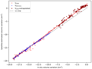
Figure 8Relationship in volume variation between satellite-estimated and in situ observations for Lake Mead, with a Pearson r > 0.99 and a NRMSE of 5.43 % (VGSW) and 1.87 % (VAltimetry).
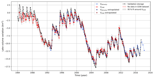
Figures 9 and 10 show the validation volume time series against the satellite-estimated volumes for Lake Mead and Lake Powell respectively. The time series showed that both the timing and magnitude of the estimated volume fluctuations were accurate for these lakes. For the non-extrapolated part of Lake Mead (2002–2016), estimated volumes were almost equal to the validation data. The extrapolated part (before 2002) was slightly overestimated (see Discussion). However, the dynamics over this period were still well captured. Lake Powell also showed accurate results, for both the seasonal and inter-annual fluctuations in water storage. Noteworthy for both lakes is the density of area observations due to a low no-data percentage in the GSW dataset. For Lake Powell, the VGSW even correctly captured seasonal fluctuations, which is not always the case (see Discussion). The high accuracy was expressed in a low NRMSE of 4.52 and 2.96 % for VGSW and VAltimetry respectively. Note that almost no extrapolated volume estimates were required for the volume time series of Lake Powell.
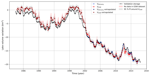
Figure 9Validation time series plotted with estimated reservoir volumes for Lake Mead. The black triangle line represents the validation storage as measured using the full lake bathymetry.
This study presented a new methodology to estimate lake and reservoir volumes using remote sensing alone. The validation showed that the method can produce water storage change estimates for many lakes, thus highlighting the potential of combining satellite altimetry and the GSW dataset to develop a global lake and reservoir volume variation dataset. The GSW dataset global coverage, 30 m resolution, high accuracy and monthly surface water observations over a 32-year period increases the number of analysed lakes and the accuracy, quantity and temporal range of lake area calculations. Therefore, volume variations can now also be calculated using GSW lake areas as input independent from altimetry data, which allows for volume calculations further back in time to 1984.
The lake and reservoir volume dataset developed here will help to better understand the behaviour and operations of lakes and reservoirs. As the number of reservoirs is still increasing because of growing energy demands, it is crucial to include their effects in (continental- and global-scale) hydrological models. Zajac et al. (2017) found that the exclusion of lakes and reservoirs often leads to inaccurate downstream discharge estimates. Furthermore, lake or reservoir storage change combined with modelled or observed inflow allows for a better estimation of the outflow (e.g. Muala et al., 2014). These outflow estimates can be used to calibrate hydrological models or estimate hydropower production in areas where in situ observations are lacking. However, due to a lack of storage observations and their availability – often because of commercial reasons – the parametrization and the representation of lakes and reservoirs in many hydrological models – if at all present – is still highly simplified. Our global lake and reservoir volume dataset over 32 years will be very beneficial to calibrate and validate their parameterization to mimic their operational behaviour. This will improve our current understanding of lakes and reservoirs, improve their simulations and consequently the simulations in the rest of the river basin. In addition, a better understanding of reservoirs will also likely improve water and energy production projections of the influence of these reservoirs under climate change, or under different management scenarios (e.g. changing downstream water requirements, flow legislation, changing inflow due to other activities upstream). Moreover, the area time series developed in this study can be included in models to improve on (often fixed) current area estimates and can furthermore improve estimates of open-water evaporation.
The methodology used in this study has a couple of limitations. They arise mainly from limitations in the input data (GSW and DAHITI altimetry dataset) and the volume calculation methodology.
5.1 Satellite altimetry limitations
The altimeter footprint can be up to 16 m over land and land influences inside this footprint can alter the water level accuracy by disturbing the altimeter waveforms (Fu and Cazenave, 2001). Water level estimations of very small lakes or reservoirs can therefore have a RMSE of several decimetres or larger (Schwatke et al., 2015a). We analysed many small lakes in Europe that did show regressions with large residuals (e.g. Thülsfelder Talsperre, 1.7 km2; Hainer See, 4 km2; Lake Resia, 6.6 km2 and Altmuehl See, 4.5 km2). However, many other factors than the size of the water body determine the accuracy of the measurement; surrounding topography, surface waves, winter ice coverage, the shape of the water body and the position of the altimeter track also determine the measurement error. This could explain why no clear relationship between lake size and size of the regression residuals (R2) was observed. Although most lakes with an area < 10 km2 showed poor results in the regression, some of these small lakes still returned a regression with low residuals (e.g. Barragem do Caia and Encoro de Salas). Water level estimations are only possible if the water body is located along mission-dependent ground tracks. Larger lakes and reservoirs were more frequently captured by a combination of satellite tracks and therefore showed more frequent observations than smaller ones.
5.2 The influence of a lack of data in lake area calculations
The classifier of the GSW dataset has been shown to be very accurate, with less than 1 % of false water detections, and less than 5 % omission (Pekel et al., 2016). Therefore, the influence of classification errors in the volume estimations was very limited.
In this methodology, no-data classifications in the GSW dataset play a much more important role. These are caused by snow, ice, cloud or sensor-related issues (e.g. white striping in Fig. 2) and are likely to give an underestimation of the actual lake area if they are inside the MWE. Therefore, their influence has been reduced with a strict no-data thresholds applied to each monthly calculation. The 1 % no-data threshold for the regression and 5 % for the volume calculation resulted in the best trade-off between the number of observations from the GSW dataset and the accuracy of the estimates. Higher no-data thresholds introduced too much variability in the volume estimates, as (1) regression lines became much noisier and (2) the area of a monthly lack of data exceeded the actual lake area variation. Locations with frequent cloud cover, lake ice coverage or sensor-related image failures will often return no-data amounts that exceed the threshold, resulting in a sparse VGSWtime series. Although they are sparse, these area volume estimates can still show an acceptable accuracy, as was observed for the Puente Nuevo Reservoir in Spain (Fig. 11). For locations in the high or low latitudes, winter months are masked due to low solar zenith angles that cause considerable shadowing. Moreover, a short period of daylight or ice and snow coverage on the water surface can further increase the no-data percentage in these regions.
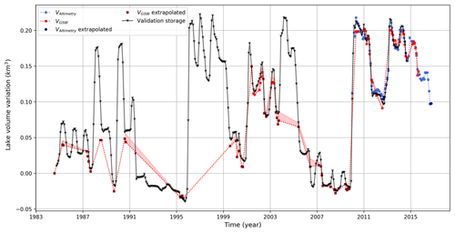
Figure 11Time series of satellite-estimated volume variations compared to validation storages for Puente Nuevo Reservoir.
Besides the varying image quality, the whole stack of historical Landsat imagery has an unequal global spatial distribution. The US and Australia are well covered, while other regions, like Africa and southwestern Europe, have much fewer Landsat observations (Pekel et al., 2016; Wulder et al., 2016). The volumetric plots of US lakes therefore typically show a highly dense VGSW, while lakes in Africa and other less monitored regions typically have more years of no observations, especially before 2000. This can clearly be observed by comparing Lake Mead and Powell (US) with Lake Nasser and Kariba (Africa) in Fig. 6. However, for lakes with sparse VGSW estimates, VAltimetry estimates still provide a valuable volume variation record.
Many layers in the GSW dataset could be used to reduce the amount of no-data pixels. This would considerably increase the capabilities of the methodology, especially in the regions mentioned above. No-data pixels that are located in the middle of the lake and are surrounded by water pixels (e.g. Fig. 2) have a high probability of being water. Furthermore, the large temporal range (1984–2015) of the GSW dataset could be used to further decrease the no-data percentage. For example, no-data pixels that are classified as water over nearly all the 380 months could be assigned to the water class with high confidence. The GSW seasonality layer could also be used to find permanent water pixels, which can be converted to water if they are not observed during a specific month.
5.3 Uncertainties and limitations in the volume calculation technique
Only 4 out of 137 lakes (Tawakoni, Urmia, Tsimlyansk and Eagle) showed a clear non-linear area–level relation. For these lakes, volume variations were not estimated. Their regressions could be explained by a second- or third-order polynomial and a hyperbolic sine function, as shown for Lake Urmia in Fig. 12. This non-linearity is caused by a considerable change in slope, which will mostly be observed for lakes with extremely low water levels (e.g. Lake Urmia) or during floods.
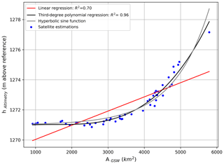
Figure 12Relationship between AGSW and hAltimetry for Lake Urmia. Only 4 out of the 137 lakes showed a clear non-linear relationship.
To reduce data size, the monthly GSW dataset does not include exact dates of the Landsat observations. This causes more uncertainty in the regression, as the level and area observations may refer to different dates (maximum difference of 1 month) and therefore to slightly different lake conditions. For lakes with a highly variable level within a month, this uncertainty therefore increases. The outliers in the regression of Lake Nasser (Fig. 4d) are expected to be largely induced by this uncertainty. For both outliers, the altimeter measurements were taken in the beginning of the month (2nd and 6th day), and the water level changed considerably by the next month. The Landsat observation therefore likely measured different lake conditions than the satellite altimeter.
For 37 lakes with lower performance, the regression showed relatively low R2 values with an average of 0.50. The most important reasons for these bad regressions were found to be winter ice or snow coverage, cloud coverage, Landsat sensor issues and multiple individual lake compartments. Winter ice coverage influences both the altimetry accuracy and the accuracy in the GSW water classification (e.g. Lake Ulungur, Rybinsk Reservoir, Reindeer Lake and Lake Ilmen). The current methodology needs to be refined to include lakes that split into multiple lakes during extreme drying (e.g. the Aral Sea). As the different compartments can have different water level dynamics, individual regressions would need to be assigned to each compartment to calculate volume fluctuations of each compartment individually. Further research on water losses in the Aral Sea using this technique could be very promising.
The calculated extrapolated volumes are more uncertain than the non-extrapolated ones, depending on how much the hypsometry relationship changes outside the regression range. In general, if the altimetry measurement period is short compared to the area time series, the range of level and area values captured by the regression line is likely to be small and the volume extrapolation using extreme area observations is expected to be less accurate. This was observed for the Roseires Reservoir and Lake Mead. The validation results for Lake Mead (Figs. 8 and 9) indicate that for large areas observed outside the regression range (1984–2002) the found linear hypsometry relationship produces slightly biased volume variation estimates. The extrapolated VGSW volumes slightly overestimate volume losses since 1984 compared to the validation data based on in situ measurements. The slight non-linearity observed in the regression of Lake Mead (see Fig. 4c) could be an indication for a stronger non-linear hypsometry relationship in the extrapolated domain. This could be a potential explanation for the slight overestimation of the losses between 1984 and 2002. The additional uncertainty induced by extrapolation cannot be fully addressed by our current uncertainty estimate using the PI. However, including extrapolated volumes hardly changed the overall validation results, because only 15 % of the volumes were estimated using extrapolation. Note that the underestimation of VGSW for Lake Powell between 1984 and 1990 is not caused by extrapolation error. This underestimation could be caused by errors in the USBR in situ validation data or by omission errors in the GSW dataset, although Pekel et al. (2016) stated the omission error to be overall less than 5 %. The exact causation of this inaccuracy remains debatable.
This study successfully combined the JRC Global Surface Water (GSW) dataset and the DAHITI satellite altimetry dataset to estimate lake and reservoir volume fluctuations over all continents. The GSW dataset records surface water over a 32-year period, containing 3 066 080 monthly images that cover 99.95 % of the landmass. The extensive size and high accuracy of this surface water dataset allowed for detailed volume variation estimations over a very long time period (1984–2015), without being constrained by complex and computationally intensive classification procedures.
Lake areas from the GSW dataset and water levels from the DAHITI altimetry dataset have been combined in a regression to explain the lake hypsometry of 137 lakes globally. Nearly all lakes showed a linear regression. A total of 58 of these lakes returned relatively low residuals with R2 > 0.8, with an average of 0.91. Lake volumes were calculated for all these lakes and for 42 other lakes with a nearly constant lake area. For 37 lakes, the regression showed higher residuals (R2 < 0.8) with an average R2 of 0.50. Winter ice coverage and a lack of data in the GSW dataset were found to be most important reasons for low R2 values.
For 100 lakes (58 with variable area and 42 with nearly constant area) volume variations were calculated by integrating the hypsometric relationships, using both area and water level observations separately. Decreases in water storage were found in the western US, where Lake Mead, Lake Powell and the Great Salt Lake lost 11, 6 and 16 km3 respectively of average volume between 1984–2000 and 2000–2015. According to our estimates, Lake Mead lost approximately 20 km3 of water from 2000 to 2015. Using the USGS in situ measured storage volume of 31 km3 in 2000, this is an almost 70 % reduction in water storage over the last 15 years. Lake volume variation estimates have been validated for 18 lakes in the US, Spain, Australia and Africa using in situ lake volume time series. The estimated volume variations showed the method to be very accurate, expressed in an average Pearson correlation coefficient of 0.97, and a normalized RMSE of 7.42 %.
The low number of adequate Landsat lake area observations for some regions like Africa and southwestern Europe still remains a limitation. Therefore, it would be highly beneficial for the purpose of this research to include surface water data from other satellites in the GSW dataset and to develop techniques to decrease the no-data percentage in the current dataset. Future plans are to include Sentinel-1 and Sentinel-2 in the GSW dataset. The DAHITI database is continuously growing by analysing new water bodies, and newly available altimetry data will be processed to expand the volumetric dataset.
This lake and reservoir volume dataset will help to improve our current understanding of the behaviour of lakes and reservoirs, their representation in hydrological models and consequently the simulations of the river basin. This will, moreover, improve projections of the river basin under climate change or under different management scenarios and improve hydropower and open-water evaporation estimations.
This study constitutes a proof of concept paving the way for increasing the number of lakes and reservoirs analysed, which could potentially be included as an a priori water storage dataset for the Surface Water and Ocean Topography (SWOT) hydrology and oceanography satellite mission. Launched in 2020, this mission will combine water body contours and accurate water level estimations to estimate storage changes in lakes and reservoirs with an average accuracy of 20 cm (Biancamaria et al., 2016; Crétaux et al., 2015). The SWOT satellite will be unique due to its accuracy and capabilities on smaller water bodies with a size of at least 250 m × 250 m.
Research outcomes (i.e. lake and reservoir volumes) are not publicly accessible. However, they may become publicly available in a later stage through the DAHITI web service (http://dahiti.dgfi.tum.de/en/, Schwatke et al., 2015, last access: 14 July 2018). The access to remote sensing data used in this study is explained in Sect. 2.
The supplement related to this article is available online at: https://doi.org/10.5194/hess-23-669-2019-supplement.
TB developed the methodology, the scripts and was the main writer of the paper. AdR helped writing the introduction section and gave comprehensive scientific support over the whole period. EG gave outstanding and extensive support in coding the scripts, developing the methodology and the uncertainty analysis during the feedback process. CS provided DAHITI altimetry data, additionally processed water bodies on demand and, moreover, wrote the altimetry section. JFP and AC contributed in the Google Earth Engine usage and wrote the GSW section. All authors actively contributed to the feedback process after the first draft.
The authors declare that they have no conflict of interest.
We would like to thank the Google Earth Engine team,
and especially Matthew Hancher and Noel Gorelick, for support in developing
the Earth Engine scripts. We would also like to express our gratitude to
Guido Lemoine (Joint Research Centre) for his technical support in Earth
Engine and Steven de Jong (Utrecht University) for his feedback on the first
report.
Edited by: Anas Ghadouani
Reviewed by: Renata Romanowicz and two anonymous referees
Avisse, N., Tilmant, A., Müller, M. F., and Zhang, H.: Monitoring small reservoirs storage from satellite remote sensing in inaccessible areas, Hydrol. Earth Syst. Sci., 21, 6445–6459, https://doi.org/10.5194/hess-21-6445-2017, 2017.
Balmer, M. and Downing, J.: Carbon dioxide concentrations in eutrophic lakes: undersaturation implies atmospheric uptake, Inl. Waters, 1, 125–132, https://doi.org/10.5268/IW-1.2.366, 2011.
Barnett, T. P. and Pierce, D. W.: When will Lake Mead go dry?, Water Resour. Res., 44, https://doi.org/10.1029/2007WR006704, 2008.
Benenati, E. P., Shannon, J. P., Blinn, D. W., Wilson, K. P., and Hueftle, S. J.: Reservoir-river linkages: Lake Powell and the Colorado River, Arizona, J. North Am. Benthol. Soc., 19, 742–755, https://doi.org/10.2307/1468131, 2000.
Berg, H., Michélsen, P., Troell, M., Folke, C., and Kautsky, N.: Managing aquaculture for sustainability in tropical Lake Kariba, Zimbabwe, Ecol. Econ., 18, 141–159, https://doi.org/10.1016/0921-8009(96)00018-3, 1996.
Biancamaria, S., Lettenmaier, D. P., and Pavelsky, T. M.: The SWOT Mission and Its Capabilities for Land Hydrology, Surv. Geophys., 37, 307–337, https://doi.org/10.1007/s10712-015-9346-y, 2016.
Biemans, H., Haddeland, I., Kabat, P., Ludwig, F., Hutjes, R. W. A., Heinke, J., von Bloh, W., and Gerten, D.: Impact of reservoirs on river discharge and irrigation water supply during the 20th century, Water Resour. Res., 47, https://doi.org/10.1029/2009WR008929, 2011.
Birkett, C. M.: The contribution of TOPEX/POSEIDON to the global monitoring of climatically sensitive lakes, J. Geophys. Res., 100, 179–25, https://doi.org/10.1029/95JC02125, 1995.
Boergens, E., Dettmering, D., Schwatke, C., and Seitz, F.: Treating the hooking effect in satellite altimetry data: A case study along the mekong river and its tributaries, Remote Sens., 8, 91–113, https://doi.org/10.3390/rs8020091, 2016.
Bosch, W., Dettmering, D., and Schwatke, C.: Multi-mission cross-calibration of satellite altimeters: Constructing a long-term data record for global and regional sea level change studies, Remote Sens., 6, 2255–2281, https://doi.org/10.3390/rs6032255, 2014.
Chao, B. F., Wu, Y. H., and Li, Y. S.: Impact of artificial reservoir water impoundment on global sea level, Science, 320, 212–214, https://doi.org/10.1126/science.1154580, 2008.
Cole, J. J., Prairie, Y. T., Caraco, N. F., McDowell, W. H., Tranvik, L. J., Striegl, R. G., Duarte, C. M., Kortelainen, P., Downing, J. A., Middelburg, J. J., and Melack, J.: Plumbing the global carbon cycle: Integrating inland waters into the terrestrial carbon budget, Ecosystems, 10, 171–184, https://doi.org/10.1007/s10021-006-9013-8, 2007.
Cook, E. R., Seager, R., Cane, M. A., and Stahle, D. W.: North American drought: Reconstructions, causes, and consequences, Earth-Sci. Rev., 81, 93–134, https://doi.org/10.1016/j.earscirev.2006.12.002, 2007.
Crétaux, J.-F., Biancamaria, S., Arsen, A., Bergé Nguyen, M., and Becker, M.: Global surveys of reservoirs and lakes from satellites and regional application to the Syrdarya river basin, Environ. Res. Lett., 10, 15002, https://doi.org/10.1088/1748-9326/10/1/015002, 2015.
Crétaux, J.-F., Abarca-del-Río, R., Bergé-Nguyen, M., Arsen, A., Drolon, V., Clos, G., and Maisongrande, P.: Lake Volume Monitoring from Space, Surv. Geophys., 37, 269–305, https://doi.org/10.1007/s10712-016-9362-6, 2016.
Downing, J. A., Prairie, Y. T., Cole, J. J., Duarte, C. M., Tranvik, L. J., Striegl, R. G., McDowell, W. H., Kortelainen, P., Caraco, N. F., Melack, J. M., and Middelburg, J. J.: The global abundance and size distribution of lakes, ponds, and impoundments, Limnol. Oceanogr., 51, 2388–2397, https://doi.org/10.4319/lo.2006.51.5.2388, 2006.
Duan, Z. and Bastiaanssen, W. G. M.: Estimating water volume variations in lakes and reservoirs from four operational satellite altimetry databases and satellite imagery data, Remote Sens. Environ., 134, 403–416, https://doi.org/10.1016/j.rse.2013.03.010, 2013.
Frappart, F., Calmant, S., Cauhopé, M., Seyler, F., and Cazenave, A.: Preliminary results of ENVISAT RA-2-derived water levels validation over the Amazon basin, Remote Sens. Environ., 100, 252–264, https://doi.org/10.1016/j.rse.2005.10.027, 2006a.
Frappart, F., Do Minh, K., L'Hermitte, J., Cazenave, A., Ramillien, G., Le Toan, T., and Mognard-Campbell, N.: Water volume change in the lower Mekong from satellite altimetry and imagery data, Geophys. J. Int., 167, 570–584, https://doi.org/10.1111/j.1365-246X.2006.03184.x, 2006b.
Frey, K. E. and Smith, L. C.: Amplified carbon release from vast West Siberian peatlands by 2100, Geophys. Res. Lett., 32, 1–4, https://doi.org/10.1029/2004GL022025, 2005.
Fu, L. L. and Cazenave, A.: Satellite altimetry and earth sciences: a handbook of techniques and applications, Academic Press, 2001.
Gao, H., Birkett, C., and Lettenmaier, D. P.: Global monitoring of large reservoir storage from satellite remote sensing, Water Resour. Res., 48, 1–12, https://doi.org/10.1029/2012WR012063, 2012.
Gorelick, N., Hancher, M., Dixon, M., Ilyushchenko, S., Thau, D., and Moore, R.: Google Earth Engine: Planetary-scale geospatial analysis for everyone, Remote Sens. Environ., 202, 18–27, https://doi.org/10.1016/j.rse.2017.06.031, 2017.
Haddeland, I., Heinke, J., Biemans, H., Eisner, S., Flörke, M., Hanasaki, N., Konzmann, M., Ludwig, F., Masaki, Y., Schewe, J., Stacke, T., Tessler, Z. D., Wada, Y., and Wisser, D.: Global water resources affected by human interventions and climate change, P. Natl. Acad. Sci. USA, 111, 3251–3256, https://doi.org/10.1073/pnas.1222475110, 2014.
Hanasaki, N., Kanae, S., and Oki, T.: A reservoir operation scheme for global river routing models, J. Hydrol., 327, 22–41, https://doi.org/10.1016/j.jhydrol.2005.11.011, 2006.
Holdren, G. C. and Turner, K.: Characteristics of Lake Mead, Arizona-Nevada, Lake Reserv. Manag., 26, 230–239, https://doi.org/10.1080/07438141.2010.540699, 2010.
Hwang, C., Guo, J., Deng, X., Hsu, H. Y., and Liu, Y.: Coastal gravity anomalies from retracked Geosat/GM altimetry: Improvement, limitation and the role of airborne gravity data, J. Geodesy, 80, 204–216, https://doi.org/10.1007/s00190-006-0052-x, 2006.
Kouraev, A. V., Zakharova, E. A., Samain, O., Mognard, N. M., and Cazenave, A.: Ob' river discharge from TOPEX/Poseidon satellite altimetry (1992–2002), Remote Sens. Environ., 93, 238–245, https://doi.org/10.1016/j.rse.2004.07.007, 2004.
LakeNet: Lake profile: Kariba, available at: http://www.worldlakes.org/lakedetails.asp?lakeid=8360 (last access: 2 January 2018), 2003.
Lehner, B. and Döll, P.: Development and validation of a global database of lakes, reservoirs and wetlands, J. Hydrol., 296, 1–22, https://doi.org/10.1016/j.jhydrol.2004.03.028, 2004.
Liu, Q.: Interlinking climate change with water-energy-food nexus and related ecosystem processes in California case studies, Ecol. Process., 5, 144 pp., https://doi.org/10.1186/s13717-016-0058-0, 2016.
Meybeck, M.: Global distribution of lakes, in Physics and Chemistry of Lakes, Spinger, Berlin, Germany, 1–35, 1995.
Micklin, P.: The future Aral Sea: hope and despair, Environ. Earth Sci., 75, 844, 1–15, https://doi.org/10.1007/s12665-016-5614-5, 2016.
Muala, E., Mohamed, Y. A., Duan, Z., and van der Zaag, P.: Estimation of reservoir discharges from Lake Nasser and Roseires Reservoir in the Nile Basin using satellite altimetry and imagery data, Remote Sens., 6, 7522–7545, https://doi.org/10.3390/rs6087522, 2014.
Pekel, J.-F., Cottam, A., Gorelick, N., and Belward, A. S.: High-resolution mapping of global surface water and its long-term changes, Nature, 540, 1–19, https://doi.org/10.1038/nature20584, 2016.
Ran, L. and Lu, X. X.: Delineation of reservoirs using remote sensing and their storage estimate: An example of the Yellow River basin, China, Hydrol. Process., 26, 1215–1229, https://doi.org/10.1002/hyp.8224, 2012.
Richey, J. E., Melack, J. M., Aufdenkampe, A. K., Ballester, V. M., and Hess, L. L.: Outgassing from Amazonian rivers and wetlands as a large tropical source of atmospheric CO2, Nature, 416, 617–620, https://doi.org/10.1038/416617a, 2002.
Schwatke, C., Dettmering, D., Bosch, W., and Seitz, F.: DAHITI – An innovative approach for estimating water level time series over inland waters using multi-mission satellite altimetry, Hydrol. Earth Syst. Sci., 19, 4345–4364, https://doi.org/10.5194/hess-19-4345-2015, 2015a.
Schwatke, C., Dettmering, D., Börgens, E., and Bosch, W.: Potential of SARAL/AltiKa for Inland Water Applications, Mar. Geod., 38, 626–643, https://doi.org/10.1080/01490419.2015.1008710, 2015b.
Schwatke, C., Dettmering, D., Bosch, W., and Seitz, F.: Database for Hydrological Time Series of Inland Waters (DAHITI), Technische Universität München, available at: http://dahiti.dgfi.tum.de/en/ (last access: 14 July 2018), 2015.
Smith, L. C. and Pavelsky, T. M.: Remote sensing of volumetric storage changes in lakes, Earth Surf. Proc. Land., 34, 1353–1358, https://doi.org/10.1002/esp.1822, 2009.
Tong, X., Pan, H., Xie, H., Xu, X., Li, F., Chen, L., Luo, X., Liu, S., Chen, P., and Jin, Y.: Estimating water volume variations in Lake Victoria over the past 22 years using multi-mission altimetry and remotely sensed images, Remote Sens. Environ., 187, 400–413, https://doi.org/10.1016/j.rse.2016.10.012, 2016.
Tourian, M. J., Schwatke, C., and Sneeuw, N.: River discharge estimation at daily resolution from satellite altimetry over an entire river basin, J. Hydrol., 546, 230–247, https://doi.org/10.1016/j.jhydrol.2017.01.009, 2017.
Verpoorter, C., Kutser, T., Seekell, D. A., and Tranvik, L. J.: A global inventory of lakes based on high-resolution satellite imagery, Geophys. Res. Lett., 41, 6396–6402, https://doi.org/10.1002/2014GL060641, 2014.
Villadsen, H., Andersen, O. B., Stenseng, L., Nielsen, K., and Knudsen, P.: CryoSat-2 altimetry for river level monitoring – Evaluation in the Ganges-Brahmaputra River basin, Remote Sens. Environ., 168, 80–89, https://doi.org/10.1016/j.rse.2015.05.025, 2015.
Wulder, M. A., White, J. C., Loveland, T. R., Woodcock, C. E., Belward, A. S., Cohen, W. B., Fosnight, E. A., Shaw, J., Masek, J. G., and Roy, D. P.: The global Landsat archive: Status, consolidation, and direction, Remote Sens. Environ., 185, 271–283, https://doi.org/10.1016/j.rse.2015.11.032, 2016.
Zajac, Z., Revilla-Romero, B., Salamon, P., Burek, P., Hirpa, F., and Beck, H.: The impact of lake and reservoir parameterization on global streamflow simulation, J. Hydrol., 548, 552–568, https://doi.org/10.1016/j.jhydrol.2017.03.022, 2017.
Zakharova, E. A., Kouraev, A. V., Cazenave, A., and Seyler, F.: Amazon River discharge estimated from TOPEX/Poseidon altimetry, Comptes Rendus Geosci., 338, 188–196, https://doi.org/10.1016/j.crte.2005.10.003, 2006.
Zhang, G., Xie, H., Kang, S., Yi, D., and Ackley, S. F.: Monitoring lake level changes on the Tibetan Plateau using ICESat altimetry data (2003–2009), Remote Sens. Environ., 115, 1733–1742, https://doi.org/10.1016/j.rse.2011.03.005, 2011.
Zhang, J., Xu, K., Yang, Y., Qi, L., Hayashi, S., and Watanabe, M.: Measuring water storage fluctuations in Lake Dongting, China, by Topex/Poseidon satellite altimetry, Environ. Monit. Assess., 115, 23–37, https://doi.org/10.1007/s10661-006-5233-9, 2006.
Zhou, Y., Jin, S., Tenzer, R., and Feng, J.: Water storage variations in the Poyang Lake Basin estimated from GRACE and satellite altimetry, Geod. Geodyn., 7, 108–116, https://doi.org/10.1016/j.geog.2016.04.003, 2016.


