Explainable Histopathology Image Classification with Self-organizing Maps: A Granular Computing Perspective

Abstract

The automatic analysis of histology images is an open research field where machine learning techniques and neural networks, especially deep architectures, are considered successful tools due to their abilities in image classification. This paper proposes a granular computing methodology for histopathological image classification. It is based on embedding tiles of histopathology images using deep metric learning, where a self-organizing map is adopted to generate the granular structure in this learned embedding space. The SOM enables the implementation of an explainable mechanism by visualizing a knowledge space that the experts can use to analyze and classify the new images. Additionally, it provides confidence in the classification results while highlighting each important image fragment, with the benefit of reducing the number of false negatives. An exemplary case is when an image detail is indicated, with small confidence, as malignant in an image globally classified as benign. Another implemented feature is the proposal of additional labelled image tiles sharing the same characteristics to specify the context of the output decision. The proposed system was tested using three histopathology image datasets, obtaining the accuracy of the state-of-the-art black-box methods based on deep learning neural networks. Differently from the methodologies proposed so far for the same purpose, this paper introduces a novel explainable method for medical image analysis where the advantages of the deep learning neural networks used to build the embedding space for the image tiles are combined with the intrinsic explainability of the granular process obtained using the clustering property of a self-organizing map.

Introduction

A fundamental approach to computing was proposed by Zadeh with the theory of granular computing (GrC). According to his point of view, the three fundamental concepts underlying human cognition are granulation, organization, and causation. Granulation is the decomposition of information into parts, organization involves the integration of granules as a whole, and causation is the association of causes with effects [1]. The idea of crisp information granulation has demonstrated usefulness in multiple related fields [2]. As Zadeh wrote, “Granulation of an object A leads to a collection of granules of A, with a granule being a clump of points (objects) drawn together by indistinguishable similarity, proximity, or functionality” [1]. Granulation involves the decomposition into sub-parts, and this process is typically due to the analysis of composing parts and the management of vague and uncertain information. An improvement is the consideration of a group of individuals rather than the individuals alone. In other cases, from structured and composite information, limited information can provide a suitable solution [2].

The aspects to be considered for the formation of the granules are the similarity, proximity, and functionality of the information granules. The formation of the granules answers the important question of why some information needs to be aggregated or, conversely, separated. The other aspect of the granular computing paradigm is computation. Some suitable methodologies, such as approximation, reasoning, and inference, extract relationships about closeness, dependency, and association to represent as much information as possible [2]. In the paper by Yao et al. [3], the authors consider the granular approach to permeate all human endeavours. Any problem is conceptualized through meaningful entities, the granules, that are used to consider the right information abstraction. Processing is then conducted on these entities, followed by communicating the results. Like the fuzzy approach, this abstraction level facilitates a human-centric elaboration.

This paper focuses on analyzing pathology images based on these premises. Specifically, digital pathology is based on the scanning and digitization of the histology slides to produce high-resolution images. The images resulting from this procedure are called whole slide images (WSI) and are usually very large: they can have a dimension of more than 80,000 $\times$ 60,000 pixels. The automatic analysis of these images is complex due to their size, posing challenges for available computational resources. Not all the image areas hold equal importance, and even if the image can be processed considering the image sub-parts, it is essential to evaluate each portion with proper contextual information.

Many solutions for analyzing these images have been proposed, including dividing the images into low-dimensional patches and utilizing deep neural networks to evaluate the presence of pathological regions. Although some solutions have shown promising results, several challenges remain to be addressed and solved.

A relevant aspect of these machine learning algorithms is their lack of explanatory support for the decisions they draw. It is notorious that the relevant results of the deep models are rarely coupled with the motivation that supports a given decision. The noticeable capability to discriminate between positive and negative samples is supported just by the good results on the validation set and good machine learning practices. Anyway, some motivation that an expert in the domain can understand must be provided with the decision. This motivation is helpful in assessing whether the patterns or portions of the image relevant to the deep black-box model align with those deemed relevant by a physician. Or, in the worst case, if the model is providing a label according to marginal and irrelevant artefacts, that gained significance due to the reduced size of the training data set, enables an informed observer to spot an error and disregard a wrong decision.

Exploiting the paradigm of granular computing and considering that the analysis of histopathology samples is a key task in detecting and monitoring cancer formations. We propose a method to process visual information for histopathology exams, focused on the proper representation to analyze the samples, providing a classification with a straightforward interpretation.

Related Works

An important feature in medical imaging is the capability to provide information to support the classification or decision process. Some information can be associated with this decision process, allowing us to interpret the operation computed by the model. Usually, in the machine learning (ML) and artificial intelligence (AI) literature, a distinction is made between interpretability and explainability. Rudin in [4] identifies a set of critical points in explainable and interpretable models. Interpretability is usually referred to as the property of the employed features to be interpretable and meaningful for an observer. On the other hand, explainability is based on an additional model that agrees with the original model and, in most cases, explains the behaviour of the original model.

There may be instances where the chosen ancillary models, chosen for explainability, are not faithful to the computation of the original model, or it can be the case that they compute a summary of predictions instead of providing a full explanation.

The present work is at the intersection of two research streams: the application of GrC, particularly in the classification of images, and the interpretability or explainability of machine learning systems.

In the following subsections, the state of the art of these two research fields is analyzed with a particular focus on interpretable machine learning systems and histopathology pattern recognition, and the last subsection will discuss some explainable and interpretable systems for histopathology image classification.

GrC in Medical Image Classification

Data representation in terms of granular information is a general paradigm that can provide useful supporting information in the data analysis domain. For this reason, this section reports and discusses some relevant granular computing approaches in image organization and classification, specifically focusing on the domain of histopathology.

Granular representation can boost the capabilities of a computational model by focusing its attention on different details in the input. The granules should be variable in size so that specific mechanisms can set the most suitable value for a single granule. Pedrycz and Homenda [5] proposed a model to justify the width of granular intervals to achieve a broad representation with semantic specificity. This involves having a large interval encompassing as much data as possible, while a narrow interval is easier to identify according to specific information. The search for the right value is addressed using multiobjective optimization techniques. The author states that the prototypes obtained through this GrC approach produce a more detailed and complete insight into the results than other techniques, such as fuzzy clustering.

Consequently, this general idea has been adopted in the field of medical imaging applications by Juszczyk et al. [6] who used a granular approach to separate the internal organs in a computer tomography image.

Recent contributions to granule representation also use a self-organizing map (SOM) to generate a granular structure on the concept space of the framework for approximate reasoning, even with a neural map of very limited dimension [7]. The advantage of the SOM is its intuitive visual features and easy pattern exploration. We got this suggestion and adopted a SOM approach in the presented paper.

In the field of image analysis, basic models of granularization exist [8]. All of them are somewhat related to image segmentation. Image segmentation is a fundamental task that is accomplished as the first step in further high-level knowledge extraction from images. Image segments are considered granules (parts of the image) that are close enough according to predefined metrics [9].

GrC has also taken advantage of deep learning methodologies [10]. In particular, the authors used a generative approach based on generative adversarial networks (GAN) to identify anomalies in breast histopathology images. The GAN maps masked images into reconstructed ones, and the comparison with the input image is accomplished to evaluate the presence of anomalies in the sample and verify the presence of tumoral regions. Considering the masks applied to the image as information granules, the technique strongly depends on the dimension of the considered masks.

Granular methods can also increase the interpretability and validity of a general machine learning model [11]. This paper presents a survey of explainable methods, particularly emphasizing methods based on General Line Coordinates. This method allows the lossless visualization of data and the discovery of the most suitable classification modes.

One of the first studies that employes granular computing in disease diagnosis was the work by Zakareya et al. [12]. The authors exploit the idea that granular computing is based on the paradigm of breaking down complex problems into smaller pieces that are easier to solve. Following this line of thought, the authors divided the medical image into small regions defined as granules and processed these pieces as information granules.

This kind of approach is somewhat similar to the one used in the present paper, with the main difference being that our approach is focused on explainability rather than on the simple usage of a deep neural network architecture adopting the principle of the GrC. In particular, we went further by clustering the image tiles, and we used the cluster centres as granules of information and also as an approximation of the distribution of the image tiles in the representation space.

One specific study of granularity in histopathology image annotations is analyzed in [13]. In the paper, it is discussed whether it is more informative to annotate regions of the image or single pixels. The experimental results confirm that the best performance in classification with deep learning networks, such as VGG16, ResNet18, and MobileNet, is obtained at the pixel-wise annotation level. Also, in the task of cancer grading, the best performance is obtained with pixel annotation and, in fewer cases, with ellipse-shaped annotation. The finer annotation is considered helpful in creating accurate visual phenotypes, such as the morphology and colour of the region of interest in contrast to its surroundings.

Explainability of Machine Learning Systems

A classical technique, used to explain the classification with deep neural network, is gradient-weighted class activation mapping (Grad-CAM) [14]. Grad-CAM is a variation of class activation mapping and is based on creating a map overlaying the input images, showing which part is relevant for a given class. This map highlights the portion of the input sample that contributes to high activation for the output class. The Grad term, in particular, is provided by the weights computed by the gradient. The gradient is the derivative of the output activation with respect to the weights vector of a chosen convolutional layer. Subsequently, a ReLU activation function is applied to clip the negative values. The regions with the highest activation values are the ones that provide the most significant contribution to label attribution. However, while the map highlights certain portions of the input images, it does not provide information about the specific features that triggered the label activation, nor does it offer a high-level description of the area.

Cynthia Rudin in [4] also proposed a different explainability technique, focused on constructing optimal logical models, and they define interpretability for specific domains.

An example from the same authors aims to find a prototypical portion of the image supporting the system’s classification decision. This explainability technique is based on how people explain the motivation of visual classification to each other. Based on prototypes of image portions, this method is implemented in [15], where a bird is classified using the portions of the bird’s body that are useful to discriminate a given bird family from others. In a special prototype system, a network is trained to provide a set of prototypical elements derived from the analysis of the bird image. Our method selects, through unsupervised learning, the portion of images that are strongly related to a class. In some measures, the trained SOM behaves like a prototype map, and the parts of test images are mapped on these prototypical elements.

Explainability in Medical Image Classification Systems

Systems for explainable or interpretable histopathology image analysis have been proposed in the recent past. These systems are mainly focused on supporting the decision of pathologists, offer a second opinion, or act as a triage support system in order to help focus on more urgent or severe cases. These systems are usually oriented to a binary classification of the pixel of the image in benign or malignant or on the identification of the tumour grade (multi-class classification).

The explainability or interpretability for this kind of system is necessary in order to make the pathologist confident in the system response, as already said in the “Explainability of Machine Learning Systems” section. Interpretability requires a transparent system, where system operation is clear and available to the user analysis. An approach based on explanation is to generate a textual justification of the classification response available for the consideration of the user. This second approach requires another system, usually a black box, that generates the explanation of the system decision, an approach that can generate unfaithful explanations [4].

In the following, we have selected systems that were mainly developed in collaboration with medical personnel with a specific focus on supporting their work.

An explainable machine learning system based on explanation generation is described in [15]. The system presented in this work contains three neural networks, one dedicated to generating and providing a textual explanation that comments on some regions of interest (ROIs) in the histopathology WSI images. The system was developed with the support of 21 pathologists.

Although the goal of this system was to deliver a “Pathologist-level interpretable whole-slide cancer diagnosis...” as declared in the title of the paper, the same paper reports that there is high variability in bladder cancer diagnosis, and the percentage of disagreement can be more than 30%. This consideration raises some doubt about the effectiveness of the explanations of this system, also considering the problems highlighted by Rudin on explanation generation [16].

The most common approaches to interpretability often rely on Grad-CAM or similar techniques. For instance, the system presented in [17] classifies the WSI images into four classes. It provides pathologists with a selection of ROI areas on the image that acts as an explanation of the decision. The system was trained using images labelled by an expert using a mask highlighting interesting regions. The system is constituted by two neural networks: one that obtains the ROI areas and another that performs the classification. The authors consider the interpretability obtained with the ROI highlighting in the input image; even if this is not a Grad-CAM system, the result is the same, and there is not a clarification of which features are responsible for the classification result. The same result is obtained from the system described in [18], but in this case, the pathologist can compare her/his own selected areas with the ROI suggested by the system and update the system.

The paper in [19] sets an interesting observation that it is difficult to decide or predict the quality of a pixel in a WSI without considering its context, so the proposed system uses two different neural networks, one that produces the embedding of the patch and the other that takes into account its context. The resulting ROIs are much more compact and connected with good accuracy. The interpretability of the system is still left to the highlighting of the ROIs, and probably the presence of this kind of context filter is helping to focus user attention, but there is not an investigation on false negatives, i.e. regions that can be too small for the context filter.

The same method, like Grad-CAM, was also used in the system proposed in [20]; in this case, it was focused on skin cancer.

Our Explainability Approach vs the Existing Ones

All the systems described above are based on highlighting image details: the first one also builds a textual explanation, while the other simply focuses on some image parts. The Grad-CAM technique is a straightforward methodology that emphasizes the details responsible for the highest output value or determines the highest gradient values. In both cases, these details influence the classification results, and these image regions are often identified as regions ROI.

As Rudin wrote, there is little information on the significance of these results or on the features of the ROI that determine their importance [16]. The method indicates some regions without explaining why they are important. Again, according to Rudin, this technique says more about the other parts of the image, the ones that are not considered important. Moreover, the highlighting of the image regions is obtained at the end of the processing chain without any information on the intermediate results.

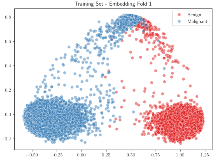
Our approach improves upon existing techniques by creating a processing chain with output that can be easily visualized and contextualized. In the following, we will see that this can help both the user and the system developers at the same time. In the proposed system, as in any other system presented above, the input image is divided into parts (tiles in our case) that are processed separately. Each tile is embedded in a space that can be visualized; Fig. 1 reports an example of this space: each dot in the figure represents a tile of the training images; the whole image is a representation of the knowledge of the system, this will further discussed in the “Construction of the Embedding Space” section.

Fig. 1

BreakHis dataset: a visualization of the embedding space in 2D, using the two most informative principal components

These tiles are organized in granules (clusters) using the SOM map, each of them labelled using the labels of the training image set. The classification of the input images is obtained by collecting all the labels of its tiles. This means that for each image, we can inspect and visualize its label (for example, in Fig. 2, the tiles classified as malignant have a red border.)

Fig. 2

Three examples of classification (left, centre, right). Each image is divided into 28 tiles. For each image, the true and predicted classes are reported (on top of each image). On the left, a benign image is correctly classified. On the centre, a malignant image is incorrectly classified as benign. On the right, there is a malignant image that is correctly classified. The red border on some tiles indicates a fragment labelled as malignant during the training phase

Compared to Grad-CAM visualization, this improves explainability because we have a classification for each image tile, indicating the quality assigned by the system. On the contrary, in the Grad-CAM system, we have a generic indication that an area is “important” for classification, and sometimes, it is said that the highlighted areas are “where the system looks”. Moreover, this classification can be explained by considering the other (training) tiles that are part of the corresponding cluster, tiles that the system considers similar to the input one. The input tiles were classified “like this” because they look similar to the tiles of the training set, a mechanism that resembles the title of the paper [16].

Methods

The proposed approach is based on the idea that some interesting areas can be spotted and characterized in histopathology images. These areas can be identified using a set of known tiles extracted from a labelled set of reference images (the training set). If a proper image embedding is produced, similarities and differences among these image tiles are translated in distances in a projection space and used during the model’s training. This projection space can be further organized using the metric learning technique, which builds a projection in a lower-dimensional space where tiles from the same class’s images are clustered together and different clusters are separated (for example, see Fig. 1). These large clusters are further divided into granules of information using the clustering property of a SOM neural network. The label of the majority of the clustered tiles will be assigned to these granules. Fragments from a test image are mapped in the embedding space and compared to granules using the Euclidean distance. The new tiles will be labelled with the closest granule.

An important aspect to consider is the performance measure in the case of a general medical image classification system for disease prediction. Performance measurement is bound with the dataset provided for this kind of study. Most of the time, public datasets for the classification of histopathology images are organized to allow images of the same patient to be in both the training set and the test set. This could artificially increase the accuracy and performance of the tested approaches, which could learn some characteristics related to a specific patient. Consequently, when possible, we chose to measure the performance of our approach in a patient-based manner. This choice reduces the number of reliable methodologies suitable for comparison.

In the following subsections, the datasets used for training and testing will be described, and the whole granular approach, composed of (1) an embedding by a triplet network, (2) a granularization by SOM, and (3) a decision paradigm, will be detailed and explained.

The Used Datasets

We face two problems in histopathological image classification: pathology classification and tumour grade identification. For the first problem, we use the BreakHis dataset [21], a benchmark dataset for classification. For the tumour grade identification, we use two different datasets: the first was proposed in [22] and collects images released by the hospital Agios Pavlos (referred to in the following sections as the Agios Pavlos dataset); the second one is the PathoIDCG dataset [23].

The BreakHis Dataset

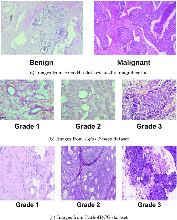
The BreakHis dataset (BH) [21] comprises images taken from sample tissue of 82 breast cancer patients. Images represent 8 pathologies: 4 benign and 4 malignant; Fig. 3a shows an image example for each class.

Fig. 3

Some images from the three datasets used

In this work, we analyze only the malignant/benign binary classification. The images in the data set have a $700 \times$460 pixels resolution and have 4 magnitude values ($40\times , 100\times , 200\times , 400\times$). According to their binary classification label, we discarded the magnification value and processed all images together, so the dataset is used as a set of 2480 benign and 5429 malignant images (Table 1). Although many authors used preprocessing techniques on input images, such as stain normalization or whitening, we do not consider any of these techniques because they could potentially compromise the extraction of important features from the input images. This choice is fully justified since our preliminary experiments show that these preprocessing techniques do not significantly increase our proposed method’s performance.

Table 1 The BreakHis dataset: for each patient, the set of images is divided in magnifications $40\times$, $100\times$, $200\times$, $400\times$. Bold indicates the best values

The original paper presenting the dataset [21] also proposes a train/test split to train a classifier. This split is based on a 70–30% proportion arranged to avoid the presence of images of the same patient in both the training set and the test set. As written above, this is very important because we found that if different images of the same patient are in both training and test, the performances are much higher (around $10\%$ increase); the separation at the patient level allows us to define the patient-level accuracy PLA, which is a specific metric for the patient and is defined in Eqs. (11) and (12).

The Agios Pavlos Dataset

The Agios Pavlos dataset [22] contains 300 images with a resolution of $1280 \times 960$ and a magnification factor of $40\times$ obtained from 21 patients with invasive ductal carcinoma. The images are labelled according to their grade: 107 images for Grade 1, 102 images for Grade 2, and 91 images for Grade 3. Figure 3b shows a sample of the pictures contained in the dataset. Through an in-depth dataset analysis, we identified nine duplicate images, i.e. those simultaneously belonging to the Grade 1 and Grade 3 classes. We decided not to consider these images, obtaining a dataset with 282 samples (Table 2 reports this new configuration). The original paper that presents the dataset [22] does not contain any information to link the images with the 21 patients. Still, looking at the prefixes of the image file names, we notice some repeated prefixes, and by grouping them, we obtain 21 groups that could be related to the patients, as we reported in Table 2. The authors of the dataset, in private communication, confirmed the connections between the image prefixes and the patient’s identity. The patient information allows us to perform a further experiment, building the training and test sets so that the images of the same patient are not simultaneously in both sets.

Table 2 The distribution of the images in the Agios Pavlos dataset before and after duplicate removal and the file name prefixes that allows to connect the images to the patients

The PathoIDCG Dataset

The PathoIDCG (Pathological Image Dataset for Invasive Ductal Carcinoma Grading) [23] contains 3644 histopathological images of invasive ductal carcinoma with a dimension of $1000 \times 1000$ and acquired at two magnification factors: $20 \times$ and $40 \times$. Each image is labelled according to its grade. In Fig. 3c, we report some examples of images, while in Table 3, we have the sample distribution divided by the magnification value.

Table 3 The distribution of the images in PathoIDCG dataset

The Embedding Space and the Granular Structure

The proposed system is based on two main components: the embedding space and the granular structure. In the first component, the input images are divided into tiles and then represented as vectors in the embedding space. This space is obtained using a neural network trained with the “metric learning” procedure. This learning algorithm moves the representations of objects of the same class near each other and moves representations of different classes far apart.

In the obtained embedding space, training tiles are roughly organized in clusters, one for each class: Fig. 1 shows the result of this phase.

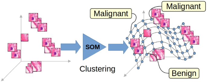
The granular structure, the second component of the system, is built in this embedding space. The SOM network creates a map of the space where are the training tiles: the SOM units are organized in a lattice that covers the embedding space, and each unit is the centre of a small cluster of similar tiles, i.e. the granules.

Construction of the Embedding Space

This subsystem aims to develop a space where histopathology images can be represented and where the classification of a new image can be obtained transparently.

The images of the three datasets used are classified as Benign and Malignant for the BreakHis dataset; Grade 1, Grade 2, and Grade 3 for the Agios Pavlos and PathoIDCG datasets. These classes should be separated in the used representation space as clearly as possible.

The first step is focused on transforming each image in the training dataset into a set of points in the embedding space. This first step is carried out in three sub-activities: first, the image is divided into tiles, then the tiles are transformed into points in a feature space, and finally, these points are projected into a lower-dimensional embedding space.

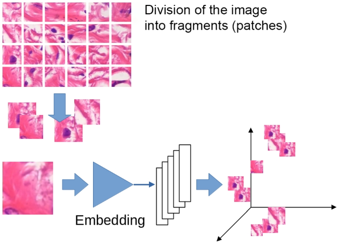
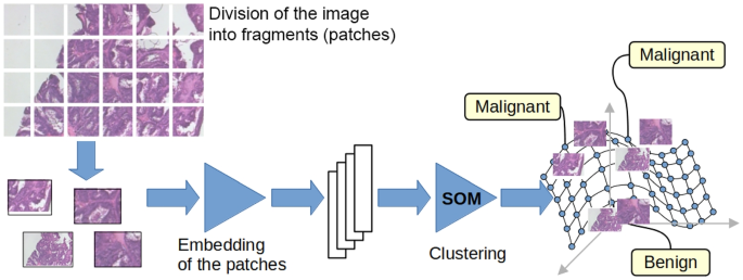
The input image is divided into tiles for many reasons: first, because we want information about parts of the image, not the whole image; second, because even if the dataset image is a patch of a larger WSI image, it is typically too big to be processed as a whole. We segment each training image into small tiles, with dimensions of $96 \times 96$ for the BreakHis and Agios Pavlos datasets and $32 \times 32$ for the PathoIDCD one. Using a pre-trained ResNet152 [24] deep neural network, these tiles are transformed into 2048-dimension vectors. These vectors are post-processed using a metric learning technique to obtain a clear cluster structure that respects the categories of the image we are interested in [25]. The metric learning technique allows us to obtain separated clusters for each class of the image: Fig. 4 shows the procedure of the division of the images in tiles and the embedding network that transforms the images into vectors in the metric space, while Fig. 1 shows the results obtained using the metric learning procedure for the BreakHis dataset. The visualization in Fig. 1 is obtained using the two most informative principal components.

Fig. 4

The construction of the embedding space; histopathology images are divided into tiles, and each fragment is projected into the embedding space. During this phase, the embedding network

We use the so-called triplet network [25] to obtain the embeddings starting from the tiles. Our proposed triplet network consists of a ResNet152 pre-trained on the ImageNet dataset [26] and a linear layer with 512 units (the embedding layer) without any activation function. We only apply the $L_2$ normalization to the obtained feature vectors in the embedding layer. The training of this kind of network requires the use of particular loss functions that consider similarity information. The goal of the embedding layer is to transform the representations $x_{*} \in \mathbb {R}^n$ to the embeddings $r_{*} \in \mathbb {R}^{n^{'}}$. According to a distance criterion d during the training procedure, the weights of the embedding layer are adjusted so that the value $d(r_a,r_n)$ is greater than a prefixed margin m w.r.t. the distance $d(r_a,r_p)$. The distance criterion d and the margin m are parameters of the model; the most commonly used distance criteria are cosine and Euclidean distances. The loss function used to train the network is the so-called triplet margin loss [27] defined as follows:

$$\begin{aligned} l_{triplet}=\max {\left\{ 0, d(r_a,r_p) - d(r_a,r_n) + m \right\} }. \end{aligned}$$

(1)

The training algorithm is organized in mini-batches, selecting the most effective triplets to update the network weights. There are several selection strategies [27]; in this work, we adopt the semi-hard negative mining strategy, defined as follows:

$$\begin{aligned} d(r_a, r_p)< d(r_a,r_n) < d(r_a,r_p) + m. \end{aligned}$$

(2)

This strategy forces the embedding of the negative examples $r_n$ to be farther away from the embedding of the anchor $r_a$ with respect to the embedding of the positive example $r_p$ but always bounded by the margin m. Consequently, the network’s loss is bounded by the margin m.

The metric learning procedure is based on training the ResNet152 representing the network, followed by a linear layer. Cluster separation is obtained during training using image triplets constituted by a reference image (anchor), a positive (same class), and a negative example (different class). Tiles inherit their label from the image they came from. Further details on the embedding into a metric space can be found in [28].

Metric learning approaches have been used successfully for medical imaging purposes [29,30,31].

Building the Granular Structure

When all training image tiles are projected in the embedding space, a clustering algorithm can be used to create a set of cluster centres that work as an upper-level structure over the image tiles.

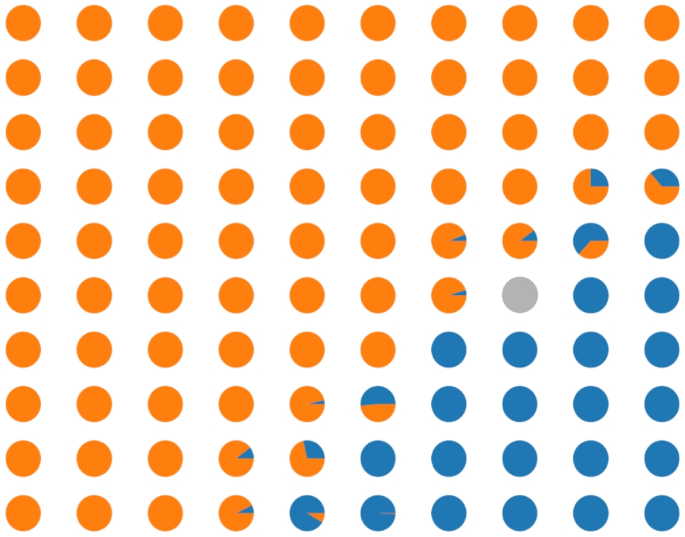
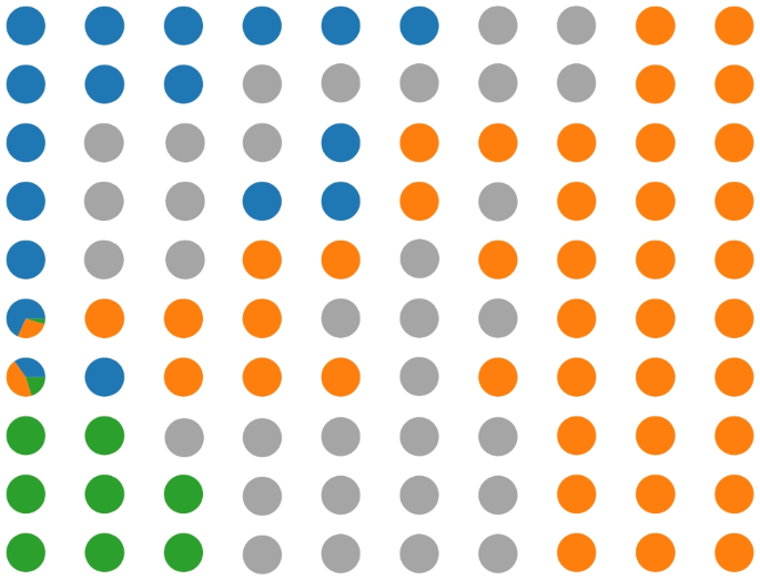
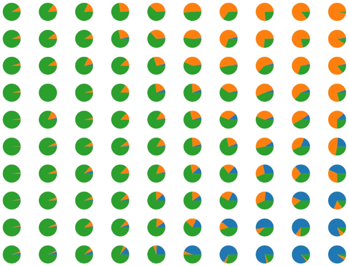
Using the self-organizing map (SOM) [32] is possible to obtain clustering without specifying the number of clusters in advance; the SOM network builds in the embedding space a lattice that contains the neural units, and this lattice constitutes the map. Figures 5, 6, and 7 show that on the map, it is possible to recognize the clusters, identified with the areas containing tiles of the same kind (i.e. areas of the same colour in the figures), sometimes separated by units that do not contain any tile (the grey units). Each neural unit in these areas groups image tiles of the same characteristics, representing a granule [33] with a measurable physical proximity to other granules in the map. This proximity guarantees a smooth feature transition from a granule to the nearest one. This combination of clustering and granular structure on a bi-dimensional lattice, which allows easy visualization, is the main reason motivating the use of SOM networks.

Fig. 5

Distribution of the tiles on the SOM map for the first fold. The grey colour indicates that the unit does not contain any tiles in the cluster; the orange colour indicates malignant tiles, and the blue colour indicates benign ones

Fig. 6

Agios Pavlos dataset: distribution of the tiles on the SOM map for the first fold. The grey colour indicates that the unit has not any tiles in the cluster. The blue indicates Grade 1 tiles, the orange Grade 2 tiles, and the green Grade 3 tiles

Fig. 7

PathoIDCG dataset: distribution of the tiles on the SOM map for the first fold. The grey colour indicates that the unit has not any tiles in the cluster. The blue indicates Grade 1 tiles, the orange Grade 2 tiles, and the green Grade 3 tiles

The SOM lattice is organized during the training phase of the network, and this phase is represented in Fig. 8. Each granule receives a label from its clustered tiles using a majority vote schema. Remember that the image tiles receive these labels from the image from which they were extracted. In a malignant image, some tiles will probably not contain “malignant details”, but this error can be neglected. The rest of the section will go deep into the training procedure.

Fig. 8

Training of the self-organizing map

As introduced before, the self-organizing map is trained using unsupervised learning to produce a two-dimensional projection called a map, preserving the relationship of proximity and distance as much as possible. SOM differs from the other neural network types because it uses competitive learning instead of error correction learning (gradient descent and back-propagation). SOM learns to recognize similar input vectors so that close neurons respond to similar input vectors. This technique is generally used to cluster, classify, and visualize the data.

A SOM consists of a series of neurons arranged in a hexagonal or rectangular lattice, a grid. Each neuron of the grid is connected with the adjacent through neighbourhood relation, dictating the map’s structure. Each map neuron can be represented as a weight vector called prototype with d features $m_i=[m_{i1}, \dots , m_{id}]$, in our case $d = 512$ because this is the dimension of the embedding space. During the training phase, for each sample r from the input dataset, the distances between r and all the map prototypes were computed. The neuron whose weight vector is closer to r is called the Best Matching Unit (BMU) and can be computed with the following equation:

$$\begin{aligned} \Vert r - m_c\Vert = \min _i{ \Vert r-m_i \Vert }. \end{aligned}$$

(3)

After the BMU finding, the weight vectors are updated so that the weight vector associated with the BMU is closest to the input vector in the input space. Furthermore, the neighbours of the BMU are treated in the same way. During the SOM training, we have two types of learning:

• Competitive learning: The prototype most similar to the input vector is updated to be more like it.

• Cooperative learning: The algorithm updates the prototype and its neighbours.

The SOM update rule for a weight vector i is as follows:

$$\begin{aligned} m_i(t+1)=m_i(t) + \alpha (t)h_{ci}(t)[r(t)-m_i(t)] \end{aligned}$$

(4)

where:

• x(t) is the input vector at time t;

• $h_{ci}(t)$ is the neighbourhood function that defines the kernel around the winner BMU c:

  $$\begin{aligned} h_{ci}(t)= \exp { \left( \frac{- d(c,i)^2}{2 \sigma ^2 (t)} \right) } \end{aligned}$$

  (5)

• $\sigma (t)$ is the neighbourhood radius at time t;

• d(c, i) is the distance between the unit c and the unit i calculated on SOM lattice;

• $\alpha (t)$ is the learning rate at time t. The learning rate can be linear $\alpha (t)=\alpha _0 \frac{1-t}{T}$ where $\alpha _0$ is the initial learning rate and T is the number of samples in the training set. Another possibility is to set the learning rate inversely proportional to time: $\alpha (t)=\frac{A}{t+B}$ with A and B suitable constants.

Before the training phase, it is necessary to initialize the weight vectors of each unit. Several strategies exist to initialize the prototypes: for example, the random strategy sets the weights with small random numbers, or the sampling strategy uses random samples of the training set. Another possibility - the one used for our experiments - is to set the SOM initial weights using the Principal Component Analysis (PCA) weights. This technique initializes the weights to span the first two principal components, doesn’t depend on random processes, and makes the training process converge faster. In Table 4, we reported the settings to train the SOM to cluster the tile representations obtained using the metric learning technique. The settings in Table 4 are the same for the three datasets involved in our experimental activity. We chose the rectangular SOM topology because a neuron has four one-neighbor neurons. This choice allows us to reduce the complexity of the proposed approach. For the radius of the neighbourhood $\sigma$, we try different values in the range [1, 10]. However, we choose $\sigma =10$ because this value allows us to obtain a more uniform granular structure with most SOM units with underlying tiles.

Note that we performed further experiments to verify whether better results are possible for the Agios Pavlos and PathoIDCG datasets, increasing the number of iterations and the $\sigma$ value. However, the results obtained are comparable to those obtained using the configuration in Table 4 (results are available upon request).

Table 4 SOM training details

The Proposed System

The proposed system can be decomposed into these sub-parts: A first subsystem extracts the tiles from the input image, a second projects them into the embedding space using the triplet network, and a following subsystem manages the granule structure supported by the SOM network. Each SOM unit is an information granule because it represents a set of similar clustered tiles and is labelled using the most common label in the cluster. Finally, a last subsystem collects all the tile labels and generates the final answer. The working and the output of each subsystem can be inspected and visualized; for example, it is possible to check the position of the tiles in the embedding space of an input image. Their position on the SOM map that implements the granular structure can be inspected, and the nearest tiles that have the most similar content can be visualized.

In the test phase, a new image will be processed by the system components (see Fig. 9): the image is divided into tiles of the same dimension as the training dataset images, and then each fragment is projected in the embedding space using the same ResNet152 network and the same projection mechanism. The embedded tiles are submitted to the SOM, which answers with a set of labels, one for each tile. At the end of the procedure, each fragment of the new image has a label, and the analysis of these labels can begin.

Fig. 9

The test phase

The system was tested for pathology identification and grade classification. Considering pathology identification, if all the tiles are classified with benign labels because they are part of granules that contain only tiles from benign images, the whole image can be classified as benign with the highest degree of certainty.

In another case, if a few tiles are in clusters with malignant labels, then we need deeper observations.

If a few tiles are labelled as malignant, an expert should further check the image; the image can still be classified as benign (because the classification mechanism uses a majority vote), but the classification is not certain, and the number of malignant tiles can be considered as an indication of the uncertainty of the classification result. If the majority of the tiles are labelled as malignant, the image can be classified as malignant. For a classification example, see the “BreakHis Dataset” section.

Regarding the grade tumour identification problem, we first counted the number of tiles in the image of each grade. Then, we labelled the image, assigning the grade corresponding to the highest number of tiles. The “Agios Pavlos Dataset” and “PathoIDCG Dataset” sections show a classification example for the Agios Pavlos and PathoIDCG datasets.

Performances Evaluation

In the general context of supervised learning, the commonly used metrics to evaluate a classification algorithm are accuracy, precision, recall (sensitivity), specificity, and F1-score. In the following, we recall the definitions of these performance indices:

$$\begin{aligned} Accuracy = \frac{TN+TP}{TN+FP+TP+FN} \end{aligned}$$

(6)

$$\begin{aligned} Precision = \frac{TP}{FP+TP} \end{aligned}$$

(7)

$$\begin{aligned} Recall \ (Sensitivity) = \frac{TP}{TP+FN} \end{aligned}$$

(8)

$$\begin{aligned} Specificity = \frac{TN}{TN+FP} \end{aligned}$$

(9)

$$\begin{aligned} F1-score = 2 \times \frac{Precision \times Recall}{Precision+Recall} \end{aligned}$$

(10)

where TP, FP, TN, and FN indicate the counting of true positives, false positives, true negatives, and false negatives, respectively. These metrics are defined for the binary classification problem. However, they can be extended to multi-class classification, averaging the results of N binary one-vs-rest classifiers, with N representing the number of classes.

If the patient information is available, classification performances will be reported using the so-called PLA [21], i.e. a performance index that takes into account the results at the patient level in the following way:

$$\begin{aligned} Patient\ Score = \frac{N_{rec}}{N_P} \end{aligned}$$

(11)

where $N_P$ is the number of images available of the patient P, and $N_{rec}$ is the fraction of $N_P$ images correctly classified. The patient-level accuracy (PLA) is defined as follows:

$$\begin{aligned} PLA = \frac{\sum {Patient \ Score}}{Total\ Number \ of \ patients} . \end{aligned}$$

(12)

The patient score is defined as the accuracy of a single patient, while PLA is an average of the patient scores, which are evaluated as an average among the patients.

Results

In this section, we describe the results obtained using our approach. For each of the three datasets considered, we first report the SOM clustering results, followed by the classification results accompanied by selected image examples.

Additionally, we performed other experiments for the BreakHis dataset. The first consists of testing the effectiveness of our proposal using ResNet152 as a feature extractor without the metric learning application. Another experiment investigates the impact of preprocessing techniques on classification by applying our approach to image processing using the stain normalization technique. To strengthen the robustness of our approach, we provide an analysis of two classical feature reduction and clustering methods, i.e. PCA and k-Means. In the embeddings obtained, we apply the PCA method to reduce the dimensionality of the data, and then we apply the k-Means algorithm to simulate the results obtained through the SOM. The last experiment consisted of classifying the images, fine-tuning the ResNet152 network, and applying the Grad-Cam technique to highlight the image regions used to assign the label to the image.

BreakHis Dataset

The proposed system was tested using the fivefold configuration described in [21]; this means that all the reported results are averaged over the five training and testing cycles.

The obtained results are reported in Table 5. The proposed technique corresponds to the row with the ML+SOM tag. A set of experiments that do not employ metric learning but just the SOM is reported in the row corresponding to NOML+SOM and shows worse results than the proposed method. For additional details, see the “Ablation Studies and Grad-Cam Comparison” section. The row SN+ML+SOM reports the results obtained using the stain normalization (SN) procedure; we carried out several experiments that can be summarized in the following steps: five different images as target images for stain normalization were selected, and for each image, the classification was performed, then an infra class stain normalization was performed, selecting five different images as a target for benign class, and five for the malignant class. In both cases, we observed no improvements in the classification accuracy. Note that the results reported in the table are obtained from only one image as the target image, which is the most used procedure when applying stain normalization.

Table 5 Comparison of results for the classification of BreakHis images between benign and malignant. ML is for metric learning; SN is for stain normalization; Acc is accuracy; Pre is precision; Se is sensitivity (recall); Spe is specificity; and F1 is F1-score. Bold indicates the best values

We have compared the proposed methodology with our last proposal, another explainable approach based on a metric space built with the same method, using the k-nearest neighbours (k-NN) classifier [28].

The comparison of the metrics (reported in Table 5) shows similar performances, but our old method classifies the image as a whole, while the new one proposed here can be able to highlight some problematic tiles in the classified image.

The system in [28] works as a reference because it is based on the same embedding space and was compared with the best system available in the literature, tested with a patient-based approach. Moreover, this method [28] has PLA performance better than or equal to all other black-box systems proposed in the literature (see the results in the paper). This allows us to make a comparison, by transitivity, of this new model with such black-box systems. In fact, the new one has even better performance in F1-score, precision, and recall than [28], proving that transparent approaches can be comparable with black-box models. These results demonstrated that there is no compromise between explainability and performance, as Rudin said in [4].

The modularity of our approach allows us to visualize the behaviour of all components of the methodology. The preliminary clustering obtained from the metric learning subsystem is reported in Fig. 1, and the results of the SOM classification are represented in Fig. 5, where each circle corresponds to a SOM unit, and the pie chart for each cell indicates the fraction of underlying malignant and benign training tiles falling in that cell. Grey units indicate units that do not have any underlying training tiles.

Figure 2 shows some classification examples: On the left, there is a benign test image correctly classified as benign. Notice that the results came from a majority vote because there are some image tiles that the method classified as malignant, highlighted with a red border, and maybe need some further investigation. The centre of the figure shows a misclassified malignant image; this is the most dangerous case because it is a false negative image. The last image shows a malignant image correctly classified as malignant.

If the tiles of a new image are not all assigned to the benign class, the user is guided to the tiles that can contain malignant details. If the user is not satisfied, they can go under the hood and check the corresponding image granules, verifying the underlying tiles. This is something that can help to correct the system’s behaviour by analyzing the “knowledge” of the system.

Agios Pavlos Dataset

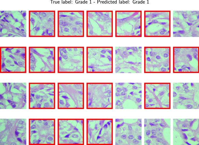
For the Agios Pavlos dataset, we performed two experiments to test the effectiveness of the proposed approach. The first involves applying a fivefold cross-validation testing protocol without considering the patient’s information, obtaining a fivefold image-based. Considering that we have patient information in the second experiment, we create fivefold patient-based images so that pictures of the same patient are not simultaneously in training and test sets. This experiment allows us to simulate a situation where the pathologist evaluates images of an unknown patient. In both experiments, during the preprocessing phase, we resize the images to $700 \times 460$ to obtain an amount of 28 patches of dimension $96 \times 96$ per image. We report the SOM results in Fig 6. Each circle represents a SOM unit, and the pie chart of each cell represents the fraction of Grade 1, Grade 2, and Grade 3 training tiles that fall into the cells. Grey circles represent the SOM unit without underlying training tiles. In Table 6, we report the classification results for both experiments that we performed. After analyzing the results, it is evident that we experienced a significant performance drop in the case of a patient-based split. In contrast, from the BreakHis experiments in which we identify the malignant tiles in the image, in this case, treating a multi-class classification problem, we identify the tiles that belong to the predicted class in the image. Figure 10 shows a correct classification of a Grade 1 image. In the figure framed in red, we have the tiles that belong to the predicted class. In this case, most tiles belong to the Grade 1 class, so our approach classifies the entire image accordingly.

Fig. 10

Agios Pavlos dataset: a correct classification of a Grade 1 image. Framed in red, we have the image tiles that belong to the predicted class

Table 6 Agios Pavlos dataset: obtained results and comparison between the proposed method and an alternative method [34]. Bold indicates the best values

We compare the results with those obtained using our previous approach introduced in [34]. In this method, we represent the histological images using a graph built starting from the tissue regions of the image. Then, we use a Graph Convolutional Neural network to perform the classification. The results obtained using this approach are in the last row of Table 6. After analyzing Table 6, it is evident that the results are comparable. However, it is essential to point out that compared to graph encoding, this new approach is computationally faster and is explainable; in fact, it provides the domain experts with the tiles used to make the final decision.

PathoIDCG Dataset

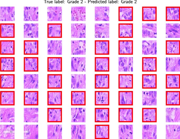
For the PathoIDCG dataset, considering that there is no predefined split between training and testing, we use a fivefold cross-validation to obtain reliable results. The images in this dataset have a resolution of $1000 \times 1000$ pixels. To make our approach applicable to these images, we resize them to $256 \times 256$ pixels and extract 64 patches of dimension $32 \times 32$. Figure 7 shows the results of the SOM clustering on the training tiles. Each circle represents a SOM unit, and the pie chart shows the distribution of the samples inside the unit. Grey circles represent the SOM unit that does match training tiles. Table 7 reports the classification performances averaged among the five folds considered. It can be seen that, in this case, our approach achieves good results in terms of accuracy but lower than those obtained for the same problem using another data set with images with a more significant dimension. In Fig. 11, we report a correct classification of a Grade 2 image.

Fig. 11

PathoIDCG dataset: a correct classification of a Grade 2 image. Framed in red, we have the image tiles that belong to the predicted class

Table 7 PathoIDCG dataset: obtained results and comparison between the proposed method and an alternative method [34]

Also, for this dataset, we compare the obtained results with those obtained in [34]. In this case, the results obtained using our new approach are worse than the previous one. The results are compared in Table 7.

Ablation Studies and Grad-Cam Comparison

In the following, we describe a set of experiments performed to demonstrate the effectiveness of the proposed approach. These experiments include using the proposed methodology without the metric learning processing for the embedding computation, using an alternative clustering approach (i.e. the combination of PCA and k-Means), and finally, using a widely employed ResNet152 combined with the Grad-Cam for the explainability. We performed all the experiments mentioned above using the BreakHis dataset. The need for metric learning is demonstrated by the ablation study, whose results are reported in the first row of Table 5. Regarding the ablation study, to obtain the fragments’ representation, we use a ResNet152 as a feature extractor without applying metric learning to create the embedding space. Then, we use the SOM to cluster the training fragments and, finally, to predict the class of test set images. Analyzing the results reported in the first two rows of Table 5, it is evident that we have a vast performance drop for all the considered metrics. This experiment clearly shows that the representation of the image fragment obtained using the pre-trained ResNet152 is needed to get good performance. Separating tiles into two groups obtained by metric learning is fundamental for subsequent grouping, and the SOM can create meaningful clusters with the ResNet152 representation obtained with metric learning.

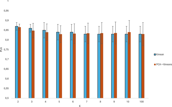
To assess the effectiveness of the use of SOM as a clustering method and dimension reduction, we conducted an analysis of two classical feature reduction and clustering methods, i.e. PCA and k-Means. First, we extracted the embeddings from the data. Then we apply the PCA to reduce the data to the first two principal components of the metric space, thus simulating the result obtained from the SOM. Then, we apply the k-Means algorithm on the fivefolds with a variable number of clusters between two and ten and compute the PLA for each of them. Additionally, we consider also one hundred clusters, which is the same number of centroids considered in the SOM. It is very important to point out that for $k>2$ the binary classification was done by considering for each test element the most frequent class within the cluster to which it is assigned. The results are shown in the Fig.  12.

Fig. 12

k-Means PLA results for $k \in [2,10]$ and $k =100$. For each k, we report the mean PLA value and its standard deviation across all folds, with or without the use of PCA features reduction. The best result is achieved at $k=2$ with PLA$=0.87$, in both cases

We report the PLA values considering just the k-Means and applying the PCA before the k-Means clustering. It may be noted that this approach provides comparable results to those obtained with the SOM model. However, unlike the method presented in this paper, k-Means can not be used to automatically determine the appropriate number of clusters, which makes it less robust than the proposed approach.

Furthermore, combining PCA and k-Means does not allow us to create a granular structure. Conversely, using our approach based on SOM clustering, we can obtain a granular structure since the SOM organizes the data topologically, i.e. it maps similar data in nearby locations on the map, capturing a more complex relationship between the data and creating a set of granules of information that reflects the intrinsic distribution of the data.

The last experiment we performed concerns the explainability mechanism and consists of classifying the images, fine-tuning the ResNet152 [24] pre-trained on the ImageNet dataset [26] with two classes, benign and malignant, and then applying the Grad-Cam approach [14]. We train the neural network for fifty epochs using the Adam optimization algorithm [35] with a learning rate $1 \times 10^{-3}$ and a mini-batch size of cardinality 32. The classification results are shown in the last row of Table 5. The Grad-Cam approach allows us to create a heatmap highlighting the image regions used to classify the image. This information will enable us to compare the explainability results obtained with our proposal with those obtained using ResNet152 with Grad-Cam.

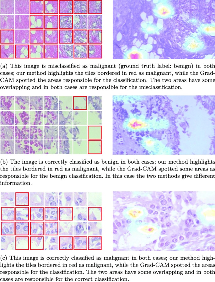
Figure 13a shows a wrong classification of a benign image. On the left, we have the results obtained using our approach, while on the right, those obtained using Grad-Cam. It is interesting to note that neither approach correctly classifies the image. Furthermore, it is possible to see a correspondence between the image’s region identified by our approach and the Grad-Cam heatmap. In Fig. 13b, we have a correctly classified benign image. In this case, both approaches correctly classify the image but provide different information: our method returns some malignant tiles—bordered in red—while Grad-Cam highlights some areas responsible for the benign classification. The two techniques are coherent since the area that Grad-Cam highlights is also benign for our method. Finally, in Fig. 13c, we report a correctly classified malignant image. In this case, we have an overlap between the regions identified by our approach and the areas highlighted using Grad-Cam. In both cases, this information is responsible for the correct image classification. It is worth noticing that while the Grad-Cam just highlights some areas of the image according to its decision process, the areas highlighted with our method are the ones that are similar to the regions of malignant regions. The tiles with red borders have patterns that are similar to areas labelled as malignant. Conversely, from the heatmap obtained through the Grad-Cam approach, only the most relevant image parts for the labelling process are highlighted. There is no identification of it as malignant. The information provided by our approach, which is a set of malignant tiles, can be helpful if integrated into a decision support system. For instance, during the examination and diagnosis process, the pathologist could use the identified malignant tiles for a more in-depth investigation or require additional exams.

Fig. 13

A comparison of our method with Grad-CAM

Discussion

From an explainability perspective, the results of our method have dual significance. As highlighted in [36], it can target either system developers or physicians, enriching the system’s responses with context.

Developers seek to comprehend and predict responses to ensure the system behaves consistently across various inputs. They also aim to identify and rectify any erratic behaviour or, at minimum, understand its causes for future avoidance. Visualizations like Fig. 1 help developers discern clear class separations within the training set, crucial for verifying the embedding phase’s outcomes. The ablation study results in Table 5 underscores this phase’s importance: poor class separation leads to diminished system performance.

The foundation of the proposed approach lies in the generalization of the embedded space shaped by the SOM network granularization. Granules receive a label from the clustered image tiles, which is used to classify the tiles of a new input image. The label received from the tiles in a BMU cell is obtained considering the classes of most tiles in the cell.

The method’s robustness is evidenced by its performance across various datasets, applicable to both binary and multi-class classifications.

Images are segmented into squared tiles of $96 \times 96$ pixels for processing. Each tile undergoes SOM network classification, with the image’s overall classification emerging from the aggregate tile classes. This method employs a voting system for each tile, with the final classification reflecting the majority. The system’s ability to handle images of any resolution and magnification level is not contingent on the number of tiles, allowing for versatile application. Further refinement of this classification process remains a topic for future research.

Figure 2 illustrates the classification of three images using a majority vote approach, where malignant tiles are marked with a red border. This method extends to multi-class classification, as depicted in Figs. 7 and 11. Notably, in the case of a malignant prediction, Fig. 3 reveals a correlation between our method’s malignant tile identification and the Grad-Cam-highlighted areas, affirming our method’s validity. Such congruence indicates that our method could excel as a decision support tool, offering dependable, interpretable insights for precise diagnosis. In addition, the classification context is provided by the training tiles within the SOM BMU, allowing users to assess the similarity and the method’s accuracy. The quantity of misclassified tiles may also indicate confidence in the results, warranting further exploration. Lastly, the label distribution within granules, as shown in Figs. 2, 5, 6, 7, and 10, offers developers insight into label consistency across tiles or if it results from majority voting.

As depicted in Figs. 2, 5, 6, 7, and 10 further insights can be gleaned from the label distribution across granules. These visualizations enable developers to discern whether a granule’s label is uniformly distributed across all tiles or if it’s the result of a majority vote.

In instances where a majority vote determines the label, the granule possesses a degree of fuzzy information that could be considered a degree of reliability. Such granules represent a mere 12% of the total, yet their inclusion in the system persists. Notably, each dataset exhibits well-demarcated classes within the SOM, ensuring coherent regional classifications.

As for performance, our method demonstrates high accuracy on the BreakHis dataset, detailed in Table 5. Interestingly, preprocessing techniques like Stain Normalization appear to offer no significant benefit to the model’s accuracy or F1-score. The superiority of using SOM for clustering and dimensionality reduction is evident when compared to traditional methods like PCA and k-Means, which, despite similar accuracy levels, lack the capability for automated cluster analysis.

The method also excels in multi-class classification scenarios, particularly in image-based settings. However, a notable performance decrease is observed in the Agios Pavlos patient-based dataset. These findings are systematically presented in Tables 6 and 7 for the Agios Pavlos and PathoIDCG datasets, respectively.

In summary, our proposed method has the potential to significantly impact future medical imaging research, serving as the cornerstone of a dependable decision support system. The granular classification data is pivotal, potentially enhancing the detection of cases warranting further investigation, such as when malignant and benign patch classifications are closely matched. Furthermore, our methodology’s simplicity ensures replicability and our provided source code can address implementation challenges. It also opens avenues for integrating our approach with others, fostering a collaborative environment among expert models.

Conclusions

This paper presented a new granular computing approach for classifying histopathology images based on image fragment extraction, metric space embedding, and SOM clustering. The results obtained on three publicly available binary and multi-class datasets are encouraging: the method has an accuracy equal to or greater than the state-of-the-art deep learning approaches based on black-box algorithms while presenting a transparent (explainability) mechanism that allows the verification of each step of the classification flow. Interestingly, this novel mechanism has shown an agreement with the Grad-Cam algorithm, a commonly used approach for convolutional networks, providing more context information and enabling a deep analysis of the classification results. It starts by classifying image tiles using a transparent mechanism and builds the classification result with a bottom-up process. Our methodology does not suffer from any accuracy vs explainability trade-off since it is intrinsically explainable due to the metric learning adoption. There is undoubtedly room for further investigations; for example, a more flexible and sophisticated procedure that considers the neighbourhood units of the SOM can be used to combine the classification of the set of tiles. The overall methodology is suitable for generic diagnostic scenarios involving images. The limitation regards the size of the input images; the bigger the image, the more patch splits are required to provide the final classification.

In addition, some insights and suggestions can come from physicians who are the final users of systems based on this approach. Due to the modularity and explainability of each component, this can significantly help improve such systems.

References

Zadeh LA. Towards a theory of fuzzy information granulation and its centrality in human reasoning and fuzzy logic. Fuzzy Sets Syst. 1997;90(2):111–27. Fuzzy Sets: Where Do We Stand? Where Do We Go?.
Yao Y, et al. Granular computing: basic issues and possible solutions. In: Proceedings of the 5th Joint Conference on Information Sciences, vol. 1. 2000. pp. 186–9.
Yao JT, Vasilakos AV, Pedrycz W. Granular computing: perspectives and challenges. IEEE Trans Cybern. 2013;43(6):1977–89.
Rudin C. Stop explaining black box machine learning models for high stakes decisions and use interpretable models instead. Nat Mach Intell. 2019;1(5):206–15.
Pedrycz W, Homenda W. Building the fundamentals of granular computing: a principle of justifiable granularity. Appl Soft Comput. 2013;13(10):4209–18.
Juszczyk J, Pietka E, Pyciński B. Granular computing in model based abdominal organs detection. Comput Med Imaging Graph. 2015;46:121–30.
D’Aniello G, Gaeta A, Loia V, Orciuoli F. A granular computing framework for approximate reasoning in situation awareness. Granul Comput. 2017;2:141–58.
Xiaona D, Chunfeng L, Baoxiang L. Research on image granulation in granular computing. In: 2020 IEEE 3rd International Conference on Information Systems and Computer Aided Education (ICISCAE). IEEE; 2020. pp. 667–74.
Liu H, Diao X, Guo H. Quantitative analysis for image segmentation by granular computing clustering from the view of set. J Algo Comput Technol. 2019;13:1748301819833050.
Mukherjee P, Pal M, Ghosh L, Konar A. A generative model based approach for zero-shot breast cancer segmentation explaining pixels’ contribution to the model’s prediction. Interpretable Artificial Intelligence: A Perspective of Granular Computing. 2021. pp. 401–25.
Kovalerchuk B, Ahmad MA, Teredesai A. Survey of explainable machine learning with visual and granular methods beyond quasi-explanations. Interpretable artificial intelligence: A perspective of granular computing. 2021. pp. 217–67.
Zakareya S, Izadkhah H, Karimpour J. A new deep-learning-based model for breast cancer diagnosis from medical images. Diagnostics. 2023;13(11):1944.
Shi J, Gao Z, Zhang H, Puttapirat P, Wang C, Zhang X, Li C. Effects of annotation granularity in deep learning models for histopathological images. In: 2019 IEEE International Conference on Bioinformatics and Biomedicine (BIBM). IEEE; 2019. pp. 2702–08.
Selvaraju RR, Das A, Vedantam R, Cogswell M, Parikh D, Batra D. Grad-CAM: why did you say that? Visual explanations from deep networks via gradient-based localization. CoRR abs/1610.02391. 2016. https://arxiv.org/abs/1610.02391.
Zhang Z, Chen P, McGough M, Xing F, Wang C, Bui M, Xie Y, Sapkota M, Cui L, Dhillon J, et al. Pathologist-level interpretable whole-slide cancer diagnosis with deep learning. Nat Mach Intell. 2019;1(5):236–45.
Chen C, Li O, Tao D, Barnett A, Rudin C, Su JK. This looks like that: deep learning for interpretable image recognition. In: Wallach H, Larochelle H, Beygelzimer A, Alché-Buc F, Fox E, Garnett R (editors) Advances in Neural Information Processing Systems, vol. 32. Curran Associates, Inc. 2019.
Zeiser FA, Costa CA, Oliveira Ramos G, Bohn HC, Santos I, Roehe AV. DeepBatch: a hybrid deep learning model for interpretable diagnosis of breast cancer in whole-slide images. Expert Syst Appl. 2021;185:115586.
Neto PC, Montezuma D, Oliveira SP, Oliveira D, Fraga J, Monteiro A, Monteiro J, Ribeiro L, Gonçalves S, Reinhard S, et al. An interpretable machine learning system for colorectal cancer diagnosis from pathology slides. NPJ Precis Oncol. 2024;8(1):56.
Wu Z, Li H, Cui L, Kang Y, Liu J, Ali H, Feng J, Yang L. Interpretable histopathology image diagnosis via whole tissue slide level supervision. In: Machine Learning in Medical Imaging: 12th International Workshop, MLMI 2021, Held in Conjunction with MICCAI 2021, Strasbourg, France, September 27, 2021, Proceedings 12. Springer; 2021. pp. 40–9.
Jiang S, Li H, Jin Z. A visually interpretable deep learning framework for histopathological image-based skin cancer diagnosis. IEEE J Biomed Health Inform. 2021;25(5):1483–94.
Spanhol FA, Oliveira LS, Petitjean C, Heutte L. A dataset for breast cancer histopathological image classification. IEEE Trans Biomed Eng. 2016;63(7):1455–62.
Dimitropoulos K, Barmpoutis P, Zioga C, Kamas A, Patsiaoura K, Grammalidis N. Grading of invasive breast carcinoma through Grassmannian VLAD encoding. PLoS One. 2017;12(9):0185110.
Yan R, Ren F, Li J, Rao X, Lv Z, Zheng C, Zhang F. Nuclei-guided network for breast cancer grading in he-stained pathological images. Sensors. 2022;22(11):4061.
He K, Zhang X, Ren S, Sun J. Deep residual learning for image recognition. In: 2016 IEEE Conference on Computer Vision and Pattern Recognition (CVPR). 2016. pp. 770–8.
Hoffer E, Ailon N. Deep metric learning using triplet network. In: Feragen A, Pelillo M, Loog M, editors. Similarity-based pattern recognition. Cham: Springer; 2015. p. 84–92.
Deng J, Dong W, Socher R, Li L-J, Li K, Fei-Fei L. ImageNet: a large-scale hierarchical image database. In: 2009 IEEE Conference on Computer Vision and Pattern Recognition. 2009. pp. 248–55.
Balntas V, Riba E, Ponsa D, Mikolajczyk K. Learning local feature descriptors with triplets and shallow convolutional neural networks. In: Wilson Richard C, Hancock ER, Smith WAP (editors) Proceedings of the British Machine Vision Conference (BMVC). 2016. pp. 1–11.
Amato D, Calderaro S, Lo Bosco G, Rizzo R, Vella F. Metric learning in histopathological image classification: opening the black box. Sensors. 2023;23(13):6003.
Calderaro S, Lo Bosco G, Rizzo R, Vella F, et al. Fuzzy clustering of histopathological images using deep learning embeddings. In: CEUR Workshop Proceedings, vol. 3074. 2022. pp. 1–9.
Calderaro S, Lo Bosco G, Rizzo R, Vella F. Deep metric learning for transparent classification of COVID-19 X-ray images. In: 2022 16th International Conference on Signal-Image Technology & Internet-Based Systems (SITIS). 2022 pp. 300–7.
Calderaro S, Lo Bosco G, Rizzo R, Vella F. Deep metric learning for histopathological image classification. In: 2022 IEEE Eighth International Conference on Multimedia Big Data (BigMM). 2022. pp. 57–64.
Kohonen T. The self-organizing map. Proc IEEE. 1990;78(9):1464–80.
Herbert JP, Yao J. A granular computing framework for self-organizing maps. Neurocomputing. 2009;72(13–15):2865–72.
Calderaro S, Lo Bosco G, Vella F, Rizzo R. Breast cancer histologic grade identification by graph neural network embeddings. In: International Work-Conference on Bioinformatics and Biomedical Engineering. Springer; 2023. pp. 283–96.
Kingma DP, Ba J. Adam: a method for stochastic optimization. 2017.
Prinzi F, Militello C, Scichilone N, Gaglio S, Vitabile S. Explainable machine-learning models for COVID-19 prognosis prediction using clinical, laboratory and radiomic features. IEEE Access. 2023;11:121492–510.
Funding
Open access funding provided by Università degli Studi di Palermo within the CRUI-CARE Agreement. This research has been supported by Project PNC 0000001 D3-4 Health - CUP B83C22006120001 and Project PNC 0000002 DARE-Digital Lifelong Prevention - CUP B53C22006460001, the National Plan for Complementary Investments to the NRRP, Funded by the European Union - NextGenerationEU. Additional support to G.L.B. has been granted by the University of Palermo FFR (Fondo Finalizzato alla ricerca di Ateneo) year 2024.
Author information
Authors and Affiliations
Contributions
Conceptualization: Salvatore Calderaro, Giosuè Lo Bosco, Riccardo Rizzo, and Filippo Vella. Methodology: Domenico Amato, Salvatore Calderaro, Giosuè Lo Bosco, Riccardo Rizzo, and Filippo Vella. Software: Domenico Amato and Salvatore Calderaro. Validation: Domenico Amato, Salvatore Calderaro, Giosuè Lo Bosco, Riccardo Rizzo, and Filippo Vella. Writing—original draft preparation: Domenico Amato, Salvatore Calderaro, Giosuè Lo Bosco, Riccardo Rizzo, and Filippo Vella. Writing—review and editing: Domenico Amato, Salvatore Calderaro, Giosuè Lo Bosco, Riccardo Rizzo, and Filippo Vella. All authors have read and agreed to the published version of the manuscript.
Corresponding author
Ethics declarations
Competing Interests
The authors declare no competing interests.
Additional information
Publisher's Note
Springer Nature remains neutral with regard to jurisdictional claims in published maps and institutional affiliations.
Rights and permissions
Open Access This article is licensed under a Creative Commons Attribution 4.0 International License, which permits use, sharing, adaptation, distribution and reproduction in any medium or format, as long as you give appropriate credit to the original author(s) and the source, provide a link to the Creative Commons licence, and indicate if changes were made. The images or other third party material in this article are included in the article's Creative Commons licence, unless indicated otherwise in a credit line to the material. If material is not included in the article's Creative Commons licence and your intended use is not permitted by statutory regulation or exceeds the permitted use, you will need to obtain permission directly from the copyright holder. To view a copy of this licence, visit http://creativecommons.org/licenses/by/4.0/.
About this article
Cite this article
Amato, D., Calderaro, S., Lo Bosco, G. et al. Explainable Histopathology Image Classification with Self-organizing Maps: A Granular Computing Perspective. Cogn Comput (2024). https://doi.org/10.1007/s12559-024-10312-1
Received:
Accepted:
Published:
DOI: https://doi.org/10.1007/s12559-024-10312-1