Composition with Knowledge Assumptions

Abstract

Zero-knowledge succinct non-interactive arguments (zk-SNARKs) rely on knowledge assumptions for their security. Meanwhile, as the complexity and scale of cryptographic systems continues to grow, the composition of secure protocols is of vital importance. The current gold standards of composable security, the Universal Composability and Constructive Cryptography frameworks cannot capture knowledge assumptions, as their core proofs of composition prohibit white-box extraction. In this paper, we present a formal model allowing the composition of knowledge assumptions. Despite showing impossibility for the general case, we demonstrate the model’s usefulness when limiting knowledge assumptions to few instances of protocols at a time. We finish by providing the first instance of a simultaneously succinct and composable zk-SNARK, by using existing results within our framework.

1 Introduction

Knowledge assumptions, a class of non-falsifiable assumptions, are often used in cases where both succinctness and extractability are required. Perhaps the most notable modern usage is in zk-SNARKs [12, 18, 20,21,22, 30, 33], which typically rely on either a knowledge-of-exponent assumption [13], the Algebraic Group Model (AGM) [17], or the even stronger Generic Group Model (GGM) [34].

The idea of utilising additional assumptions for extraction extends outside of what it traditionally considered a “knowledge assumption” to extractable functions, notably extractable one-way functions [9, 10], and extractable hash functions [4]. Arguably, one of the main benefits of the random oracle model, one of the most common “non-standard” assumptions, is to provide extractability.

The typical statement of these assumptions is that for every adversary there exists a corresponding extractor, such that when both are given the same inputs and randomness, the extractor can provide meaningful information about how the output of the adversary was created. In the Algebraic Group Model, for instance, the extractor will show how to represent the adversaries output as powers of input group elements, and in extractable hash functions it will provide a preimage to the output hash.

This is formalised as a security game, which is then assumed to hold axiomatically. The existence of the extractor may be used in a security proof to demonstrate the existence of a preimage. At the same time, a one-wayness property can be asserted, with this differing subtly from extraction in that an adversary to one-wayness does not have access to the input and randomness to extract from. This methodology has seen success in proving the security of various interesting primitives, such as non-malleable codes [27], and SNARKs.

Proving these primitives’ security under composition would typically involve using one of a number of off-the-shelf compositional frameworks, such as Universal Composability [8] or Constructive Cryptography [31], specifying an ideal behaviour for the primitive, and constructing a simulator which coerces the ideal behaviour to mimic that of the actual protocol. This simulator will naturally need to make use of the extraction properties, often to infer the exact ideal intent behind adversarial actions. It is in this that the conflict between extraction and compositional frameworks arises: As the extraction is white-box, the simulator requires the input of its counter-party – the environment, or distinguisher, of the simulation experiment. This cannot be allowed however, as it would give the simulator access to all information in the system¹, not just that of the adversary.

This conflict has been observed before in the literature, for instance in [28]. Often, the remedy is to extend the original protocol with additional components to enable the simulator to extract “black-box”, i.e. without the original inputs. For example, the Fischlin transform [15] uses multiple queries to a random oracle to bypass the inability to extract from the commitment phase of an underlying Sigma protocol, which would allow using the simpler Fiat-Shamir transform [14] instead. C$\emptyset$C$\emptyset$ [28] extends zk-SNARKs with an encryption of the witness, and a proof of correctness of this encryption to a public key the simulator can control.

A primary downside of these approaches is that (witness) succinctness is usually lost – size being limited by the information-theoretic reality of black-box witness extraction. Thus C$\emptyset$C$\emptyset$ proofs are longer than their witnesses, and UC-secure commitments [11] are longer than the message domain. A secondary one is the necessity of adding an encryption to the implementation of a primitive where no decryption would be needed; in theory this is harmless but in practice, it adds complexity without a functional purpose (beyond its usefulness in the security argument).

The above limitation can often be bypassed by using a local random oracle, as this does permit extraction. Restricting the model to allow the adversary to perform only specific computations on knowledge-implying objects, could be one way to generalise this approach. Just as a random oracle functionality would abstract over extractable hash functions, a generic group functionality would abstract over knowledge of exponent type assumptions. This would constitute a far stronger assumption however, running counter to recent developments to relax assumptions, such as the Algebraic Group Model [17], which aim for a more faithful representation of knowledge assumptions.

Our contributions. We present the first composability framework that can overcome the above limitations in terms of implementation complexity and succinctness while being reasonably accommodating to more realistic models of computation compared to the random oracle model. In terms of applications, our approach suggests a viable direction for the composable design of SNARKs, a topic of current high interest due to their application in blockchain protocols (with prominent examples including privacy-preserving blockchains, such as [2, 26], blockchain interoperability [19] and scalability [16]), without sacrificing their succinctness, something infeasible with previous compositional approaches.

In more details, our work builds on the Algebraic Group Model approach and explores its consequences for composition. Our contributions are two-fold: We distill a notion of knowledge assumptions suitable for composable analyses, and present a framework allowing their usage in composable security proofs.

First, we define the concept of knowledge-respecting distinguishing environments, which we will call distinguishers, to be consistent with the terminology of Constructive Cryptography. We use the Constructive Cryptography framework [31] as an orientation point for this work, due to its relative simplicity compared to the many moving parts of UC [8], making it easier to re-establish composition after making sweeping changes to the model, as we do in this paper.

Similar to an algebraic algorithm, distinguishers in our model need to explain how they computed each knowledge-implying object they produce. We show how to extend a compositional framework by giving the simulator access to these explanations. For this purpose, we attach a type system to messages sent in the composition framework, which can mark which parts of messages imply further knowledge. The knowledge assumption is used to transform individual nodes in the network into corresponding nodes which also output this implied knowledge to a repository, which the simulator has oracle access to.

We re-establish well-known composition results with support for typed messages, and sets of valid distinguishers. The latter constrains the generality of the composition, but is what enables the usage of knowledge assumptions, as they require the distinguishers to be well-behaved.

Our second contribution investigates under which conditions it is reasonable to assume knowledge-respecting distinguishers. To this end, we define stronger versions of knowledge assumptions that depend on auxiliary and knowledge-implying inputs. These assumptions suffice to extend a distinguisher with an extractor providing said explanations.

Within this setting we are able to establish not only an impossibility result on full general composition, but more interestingly a positive result on the composition of systems relying on different knowledge assumptions. Intuitively: You can use a knowledge assumption only once, or you need to ensure the various uses do not interfere with each other (specifically, the simulators of both invocations cannot provide any advantage due to extraction, as shown in the example in Sect. 5). This result has the immediate effect of enabling the usage of primitives relying on knowledge assumptions in larger protocols – provided the underlying assumption is not used in multiple composing proofs.

We demonstrate the power of the framework by presenting a composable NIZK, which can be realised by any extractable zk-SNARK scheme with simulation extractability relying on the AGM. Notably, this is true of Groth’s zk-SNARK [1, 20]. To our knowledge, this is the first time a SNARK has been demonstrated to be composably secure without costly modifications to add black-box extraction. We additionally demonstrate that this may be combined with a protocol to securely instantiate an updateable reference string, when used with SNARKs supporting this, demonstrating that despite general-case impossibility, special composition cases that are highly relevant to current applications are provable within the framework.

2 Modelling Knowledge Assumptions

We formally define knowledge assumptions over a type of knowledge-implying objects X. When an object of the type X is produced, the assumption states that whoever produced it must know a corresponding witness of the type W. The knowledge of exponent assumption is an example of this, where X corresponds to pairs of group elements, and W is an exponent. A relation $\mathcal {R}\subseteq X \times W$ defines which witnesses are valid for which knowledge-implying objects.

In the case of the knowledge of exponent assumption, it roughly states that given a generator, and a random power s of the generator, the only way to produce a pair of group elements, where one is the sth power of the other, is to exponentiate the original pair, and in so doing implying knowledge of this exponent. There is one extra item needed: The initial exponent s needs to be sampled randomly. Indeed, this is true for any knowledge assumption: The all-quantification over potential distinguishers implies the existence of distinguishers which “know” objects in X without knowing their corresponding witness. To avoid this pre-knowledge, we assume X itself is randomly selected at the start of the protocol. For this purpose, we will assume a distribution $\mathsf {init}$, which given a source of public randomness (such as a global common random string), produces public parameters $\mathsf {pp}$, which parameterise the knowledge assumption. In the case of knowledge of exponent, this needs to sample an exponent s, and output the pair $(g, g^s)$. For this particular setup, public randomness is insufficient.

Beyond this, users do not operate in isolation: If Alice produces the pair $(g^x, g^{xs})$, knowing x and transmits this to Bob, he can produce $(g^{xy}, g^{xys})$ without knowing xy. This does not mean that the knowledge assumption does not hold, however it is more complex than one might originally imagine: One party can use knowledge-implying objects from another user as (part of) their own witnesses. Crucially this needs to be limited to objects the user actually received: Bob cannot produce $(g^{sy}, g^{s^2y})$ for instance, as he never received $(g^s, g^{s^2})$, and does not know s. This setting also lends itself more to some interpretations of knowledge assumptions than others. For instance, the classical knowledge-of-exponent assumption [13] does not allow linear combinations of inputs, while the t-knowledge-of-exponent assumption [23] does. When used composably, the latter is more “natural”, in much the same way that IND-CCA definitions of encryption fit better into compositional frameworks than IND-CPA ones, due to them already accounting for part of the composable interaction.

Definition 1

(Knowledge Assumption). A knowledge assumption ${\mathfrak {K}}$ is defined by a tuple $(\mathsf {init}, X, W, \mathcal {R})$ consisting of:

• 1. $\mathsf {init}$, a private-coin distribution to sample public parameters $\mathsf {pp}$ from, which the others are parameterised by.

• 2. $X_{\mathsf {pp}}$, the set of all objects which imply knowledge.

• 3. $W_{\mathsf {pp}}$, the set of witnesses, where $\forall x \in X_{\mathsf {pp}} : (\textsc {input}, x) \in W_{\mathsf {pp}}$.

• 4. $\mathcal {R}_{\mathsf {pp}} : (I \subseteq X_{\mathsf {pp}}) \rightarrow (Y \subseteq (X_{\mathsf {pp}} \times W_{\mathsf {pp}}))$, the relation new knowledge must satisfy, parameterised by input objects, where

  $$\forall x, y \in X_{\mathsf {pp}}, I \subseteq X_\mathsf {pp} : (x, (\textsc {input}, y)) \in \mathcal {R}_\mathsf {pp}(I) \iff x = y \wedge x \in I.$$

$\mathcal {R}_\mathsf {pp}$ must be monotonically increasing: $\forall I \subseteq J \subseteq X_\mathsf {pp}: \mathcal {R}_{\mathsf {pp}}(I) \subseteq \mathcal {R}_{\mathsf {pp}}(J).$

The inclusion of $(\textsc {input}, x)$ in $W_\mathsf {pp}$ and $\mathcal {R}_\mathsf {pp}$ for all $x \in X_\mathsf {pp}$ ensures that parties are permitted to know objects they have received as inputs, without needing to know corresponding witnesses. Importantly, this is possible only for inputs, and not for other objects. For each knowledge assumption ${\mathfrak {K}}$, the assumption it describes is in a setting of computational security, with a security parameter $\lambda$. Broadly, the assumption states that, for a restricted class of “${\mathfrak {K}}$-respecting” adversaries, it is possible to compute witnesses for each adversarial output, given the same inputs.

Assumption 1

(${\mathfrak {K}}$-Knowledge). The assumption corresponding to the tuple ${\mathfrak {K}}= (\mathsf {init}, X, W, \mathcal {R})$ is associated with a set of probabilistic polynomial time (PPT) algorithms, $\mathsf {Resp}_{\mathfrak {K}}$. We will say an algorithm is ${\mathfrak {K}}$-respecting if it is in $\mathsf {Resp}_{\mathfrak {K}}$. This set should contain all adversaries and protocols of interest. The ${\mathfrak {K}}$-knowledge assumption itself is then that, for all $\mathcal {A}\in \mathsf {Resp}_{\mathfrak {K}}$, there exists a PPT extractor $\mathcal {X}$, such that:

$$\begin{aligned} \Pr \left[ \begin{aligned}&\mathsf {pp} \xleftarrow {r}\mathsf {init}; \\&\exists I \subseteq X_\mathsf {pp}, \mathsf {aux} \in \{0, 1\}^* :\\&\mathrm {Game~1}(\mathcal {A}_{r'}, \mathcal {X}_{r'}, \mathsf {pp}, I, \mathsf {aux}) \end{aligned}\right] \le \mathrm {negl}(\lambda ), \end{aligned}$$

where $\mathcal {A}_{r'}$ and $\mathcal {X}_{r'}$ are $\mathcal {A}$ and $\mathcal {X}$ supplied with the same random coins $r'$ (as such, they behave deterministically within Game 1).

While it is trivial to construct adversaries which are not ${\mathfrak {K}}$-respecting by encoding knowledge-implying objects within the auxiliary input, these trivial cases are isomorphic to an adversary which is ${\mathfrak {K}}$-respecting, and which receives such encoded objects directly. We therefore limit ourselves to considering adversaries which communicate through the “proper” channel, rather than covertly. In this way, we also bypass existing impossibility results employing obfuscation [7]: We exclude by assumption adversaries which would use obfuscation.

Game 1

(Knowledge Extraction). The adversary $\mathcal {A}_r$ wins the knowledge extraction game if and only if it outputs a series of objects in $X_\mathsf {pp}$, for which the extractor $\mathcal {X}_r$ fails to output the corresponding witness:

$$\begin{aligned} \mathrm {let~} \vec {x} \leftarrow \mathcal {A}_r(I, \mathsf {aux}), \vec {w} \leftarrow \mathcal {X}_r(I, \mathsf {aux}) \mathrm {~in~} \vec {x} \in X_\mathsf {pp}^* \wedge \bigvee _{i = 1}^{|\vec {x}|} (x_i, w_i) \notin \mathcal {R}_\mathsf {pp}(I). \end{aligned}$$

Crucial for composition are the existential quantifications, which combined state that we assume extraction for all of the following:

This makes knowledge assumptions following Assumption 1 stronger than their typical property-based definitions. It is also non-standard as a result, as it relies on quantifiers within a probability experiment. While the adversarial win condition is well-defined, it is not necessarily computable. Nevertheless, quantifications are required for their usage in composable proofs.

2.1 Examples of Knowledge Assumptions

To motivate this definition, we demonstrate that it can be applied to various commonly used knowledge assumptions, including the knowledge of exponent assumption, the Algebraic Group Model and variants, and even to random oracles. We detail our flavour of the AGM here, and leave the details of the others to the full version of this paper [24, Appendix E]. Witnesses naturally seem to form a restricted expression language describing how to construct a knowledge-implying object. A more natural way to express the relation $\mathcal {R}$ is often an evaluation function over witnesses, returning a knowledge-implying object.

The Algebraic Group Model. Assuming a distribution $\mathsf {groupSetup}$ providing a group $\mathbb {G}$ and a generator g, we can recreate the Algebraic Group Model [17] as a knowledge assumption fitting Definition 1:

$$\begin{aligned} \begin{array}{llr} \begin{aligned} {\mathfrak {K}}_\mathsf {AGM} &{}:=(\mathsf {init}, X, W, \mathcal {R})\\ \mathsf {init} &{}:=\mathsf {groupSetup}\\ X &{}:=\mathbb {G}\end{aligned} &{}\qquad \qquad \qquad \,&{} \begin{aligned} W :=\;&{} \{\;(\textsc {op}, a, b) \mid a, b \in W\;\}\;\cup \\ &{} \{\;(\textsc {input}, i)\mid i \in X\;\}\;\cup \\ &{} \{\;\textsc {generator}\;\} \end{aligned} \end{array} \end{aligned}$$

$$\begin{aligned}\begin{gathered} \mathsf {eval}(I, w) :={\left\{ \begin{array}{ll} \mathsf {eval}(g) \circ \mathsf {eval}(h) &{} \quad \mathrm {if~} w = (\textsc {op}, g, h) \\ i &{} \quad \mathrm {if~} w = (\textsc {input}, i) \wedge i \in I \\ g &{} \quad \mathrm {if~} w = \textsc {generator} \end{array}\right. }\\ (x, w) \in \mathcal {R}(I) \iff x = \mathsf {eval}(I, w) \end{gathered}\end{aligned}$$

3 Typed Networks of Random Systems

While it is not our goal to pioneer a new composable security framework, existing frameworks do not quite fit the needs of this paper. Notably, Universal Composability [8] has many moving parts, such as session IDs, control functions and different tapes which make the core issues harder to grasp. Constructive Cryptography [31] does not have a well-established notion of globality and makes variable numbers of interfaces difficult to implement, which make the transformations we will later perform trickier.

Furthermore, the analysis of knowledge assumptions benefits from a clear type system imposed on messages being passed – knowing which parts of messages encode objects of interest to knowledge assumptions (and which do not) makes the analysis more straightforward. Due to both of these reasons, we construct a compositional framework sharing many similarities with Constructive Cryptography, however using graphs (networks) of typed random systems as the basic unit instead of random systems themselves. Crucially, when we establish composition within this framework, we do so with respect to sets of valid distinguishers. This will allow us to permit only distinguishers which respect the knowledge assumption.

Our definitions can embed existing security proofs in Constructive Cryptography, and due to the close relation between composable frameworks, likely also those in other frameworks, such as UC. Notably, our results directly imply that primitives proven using knowledge assumptions under this framework can be directly used in place of hybrids in systems proven in Constructive Cryptography.

3.1 Type Definition

We introduce a rudimentary type system for messages passed through the network. For a casual reader, the details of this are unimportant – understanding that the type system allows filtering which parts of messages are relevant to a knowledge assumption and which aren’t is sufficient to follow our construction.

Nevertheless, we formally define our type system as consisting of a unit type ${\mathbbm {1}}$, empty type ${\mathbb {0}}$, sum and product types $\tau _1 + \tau _2/\tau _1 \times \tau _2$, and the Kleene star $\tau ^*$. This type system was chosen to be minimal while still:

• 1. Allowing existing protocols to be fit within it. As most of cryptography operates on arbitrary length strings, $({\mathbbm {1}}+ {\mathbbm {1}})^*$, or finite mathematical objects, ${\mathbbm {1}}+ \ldots + {\mathbbm {1}}$, these can be embedded in the type system.

• 2. Allowing new types to be embedded in larger message spaces. The inclusion of sum types enables optional inclusion, while product types enables inclusion of multiple instances of a type alongside auxiliary information.

We stress that this type system may be (and will!) extended, and that a richer system may make sense in practice. Types follow the grammar

$$\begin{aligned} \tau \equiv {\mathbb {0}}\mid {\mathbbm {1}}\mid \tau _1 + \tau _2 \mid \tau _1 \times \tau _2 \mid \tau ^*, \end{aligned}$$

and the corresponding expression language follows the grammar

$$\begin{aligned} E \equiv \top \mid \mathsf {inj}_1(E) \mid \mathsf {inj}_2(E) \mid (E_1, E_2) \mid \epsilon \mid E_1\,{:}{:}\,E_2. \end{aligned}$$

We will also use $\mathbb {2}$ to represent ${\mathbbm {1}}+ {\mathbbm {1}}$, and 0 and 1 for $\mathsf {inj}_1(\top )$ and $\mathsf {inj}_2(\top )$ respectively. Formally, the typing rules are:

Note that there is no means to construct the empty type ${\mathbb {0}}$.

Knowledge assumptions. We expand this basic type system by allowing objects to be annotated with a knowledge assumption. Specifically, given a knowledge assumption ${\mathfrak {K}}= (\mathsf {init}, X, W, \mathcal {R})$, where $\mathsf {init}$ returns $\mathsf {pp} : \tau$, and for all $\mathsf {pp}$ in the domain of $\mathsf {init}$, both $X_\mathsf {pp}$ and $W_\mathsf {pp}$ are valid types, there are two additional types present:

• 1. The type of knowledge-implying objects in ${\mathfrak {K}}$: $[{\mathfrak {K}}_\mathsf {pp}]$ (equivalent to $X_\mathsf {pp}$)

• 2. The type of witnessed objects in ${\mathfrak {K}}$ with respect to an input set of knowledge I: $\forall I \subseteq X_\mathsf {pp} : \langle {\mathfrak {K}}_\mathsf {pp}, I \rangle$ (equivalent to $X_\mathsf {pp} \times W_\mathsf {pp}$)

Formally then, we define ${\mathfrak {K}}$ types through the grammar

$$\tau \equiv {\mathbb {0}}\mid {\mathbbm {1}}\mid \tau _1 + \tau _2 \mid \tau _1 \times \tau _2 \mid \tau ^* \mid [{\mathfrak {K}}_\mathsf {pp}] \mid \langle {\mathfrak {K}}_\mathsf {pp}, I \rangle ,$$

with the corresponding expression grammar being

$$\begin{aligned} E \equiv \top \mid \mathsf {inj}_1(E) \mid \mathsf {inj}_2(E) \mid (E_1, E_2) \mid \epsilon \mid E_1 \,{:}{:}\, E_2 \mid [E]_{\mathfrak {K}_\mathsf {pp}}\mid \langle E \rangle ^I_{\mathfrak {K}_\mathsf {pp}}. \end{aligned}$$

Crucially, the types of messages may depend on prior interactions. This is particularly obvious with the set of input knowledge I, which will be defined as the set of all previously received $x : [{\mathfrak {K}}_\mathsf {pp}]$, however it also applies to $\mathsf {pp}$ itself, which may be provided from another component of the system. This allows for the secure sampling of public parameters, or delegating this to a common reference string (CRS). The typing rules are extended with the following two rules, where $X_\mathsf {pp}$ and $W_\mathsf {pp}$ are type variable:

3.2 Random Systems

We use the same basic building-block as Constructive Cryptography [31]: Random systems [32]. We briefly recap this notion:

Definition 2

An $(\mathcal {X}, \mathcal {Y})$-random system $\mathbf {F}$ is an infinite sequence of conditional probability distributions $P^\mathbf {F}_{Y_i \mid X^iY^{i-1}}$ for $i \ge 1$, where X and Y distribute over $\mathcal {X}$ and $\mathcal {Y}$ respectively.

Specifically, random systems produce outputs in the domain $\mathcal {Y}$ when given an input in $\mathcal {X}$, and are stateful – their behaviour can depend on prior inputs and outputs. [31] itself works with random systems based on an automaton with internal state; such an automaton can then also be constrained to a reasonable notion of feasibility, such as being limited to a polynomial number of execution steps with respect to some security parameter.

We will not go into depth on modelling computational security, as it is not the primary focus of this paper, however we will assume the existence of a feasibility notion of this type. We follow the approach of [29], and consider random systems as equivalence classes over probabilistic systems. We make a minor tweak to the setting of [31] as well, and use random-access machines instead of automata.

3.3 Typed Networks

We will consider networks of random systems (which can be considered as labelled graphs) as our basic object to define composition over.

Definition 3

(Cryptographic Networks). A typed cryptographic network is a set of nodes N, satisfying the following conditions:

• 1. Each node $n \in N$ is a tuple $n = (I_n, O_n, \tau _n, R_n, A_n)$ representing:

  • $I_n$ a set of available input interfaces.

  • $O_n$ a set of available output interfaces.

  • $\tau _n : I_n \cup O_n \rightarrow T$, a mapping from interfaces to their types.

  • $R_n$, a $\left( \sum _{i \in I_n} \tau _n(i), \sum _{o \in O_n} \tau _n(o)\right)$ random system.

  • $A_n \subseteq I_n \cup O_n$, the subset of interfaces which behave adversarially.

• 2. Both input and output interfaces are unique within the network:

  $$\forall a, b \in N : a \ne b \implies I_a \cap I_b = \varnothing \wedge O_a \cap O_b = \varnothing .$$

• 3. Matching input and output interfaces define directed channels in the implied network graph. Therefore, where $a, b \in N, i \in O_a \cap I_b$:

  • The interface types match: $\tau _a(i) = \tau _b(i)$.

  • The edges have a consistent adversariality: $i \in A_a \iff i \in A_b$.

We denote the set of all valid cryptographic networks by $\mathfrak {N}$.

This corresponds to a directed network graph whose vertices are nodes, and whose edges connect output interfaces to their corresponding input interface.

Composing multiple such networks is a straightforward operation, achieved through set union. While the resulting network is not necessarily valid, as it may lead to uniqueness of interfaces being violated, it can be used to construct any valid network out of its components. We also make use of a disjoint union, $A \uplus B$, by which we mean the union of A and B, while asserting that A and B are disjoint. Due to the frequency of its use, we will allow omitting the disjoint union operator, that is, we write AB to denote $A \uplus B$.

Definition 4

(Unbound Interfaces). In a typed cryptographic network N, the sets of unbound input and output interfaces, written I(N) and O(N), respectively, are defined as the set of all tuples $(i, \tau )$ for which there exists $a \in N$ and $i \in I_a$ (resp. $i \in O_a$), where for all $b \in N$, $i \notin O_b$ (resp. $i \notin I_b$), with $\tau$ being defined as its type, $\tau _a(i)$. Furthermore, ${IO}_{\mathcal {H}}(N)$ is defined as the unbound honest interfaces: all $(i, \cdot ) \in I(N) \cup O(N)$, where i is honest, that is, where $\forall a \in N : i \notin A_a$.

We can define a straightforward token-passing execution mechanism over typed cryptographic networks, which demonstrates how each network behaves as a single random system.² We primarily operate with networks instead of reducing them to a single random system to preserve their structure: It allows easily applying knowledge assumptions to each part, and enables sharing components in parallel composition, a requirement for globality.

Definition 5

(Execution). A typed cryptographic network N, together with an ordering of I(N) and O(N) defines a random system through token-passing execution, with the input and output domains $\sum _{(\cdot , \tau ) \in I(N)} \tau / \sum _{(\cdot , \tau ) \in O(N)} \tau$, respectively. Execution is defined through a stateful passing of messages – any input to N will be targeted to some $(i, \cdot ) \in I(N)$. The input is provided to the random system $R_a$, for which $i \in I_a$. Its output will be associated with an $o \in O_a$. If there exists a $b \in N$ such that $o \in I_b$, it is forwarded to $R_b$, continuing in a loop until no such node exists. At this point, the output is associated with $(o, \cdot ) \in O(N)$ (note that, if $O(N) = \varnothing$, the corresponding random system cannot be defined, as it has an empty output domain), and is encoded to the appropriate part of the output domain.

The full version of this paper [24, Appendix A] goes into more detail on the semantics, formally describing the functions $\mathsf {exec}(N, i, x)$ and $\mathsf {execState}(N, i, x, \varSigma )$. In order to help with preventing interface clashes, we introduce a renaming operation.

Definition 6

(Renaming). For a cryptographic network N, renaming interfaces $a_1, \ldots , a_n$ to $b_1, \ldots , b_n$, is denoted by:

Where, for $m = (I_m, O_m, \tau _m, \cdot , A_m)$, $m[a_1/b_1,\ldots ,a_n/b_n]$ is defined by replacing each occurrence of $a_i$ in the sets $I_m$, $O_m$ and $A_m$ with the corresponding $b_i$, as well as changing the domain of $\tau _m$ to accept $b_i$ instead of $a_i$, with the same effect.

To ensure renaming does not introduce unexpected effects, we leave it undefined when any of the output names $b_i$ are present in the network N, and are not themselves renamed (i.e. no $a_j$ exists such that $a_j = b_i$). Likewise, we prohibit renaming where multiple output names are equal. For a set of cryptographic networks, the same notation denotes renaming on each of its elements.

When talking about valid distinguishers, these are sets of cryptographic networks closed under internal renaming.

Definition 7

(Distinguisher Set). A set of distinguishers $\mathfrak {D}\subseteq \mathfrak {N}$ is any subset of $\mathfrak {N}$ which is closed under internal renaming: For any $D\in \mathfrak {D}, \vec {n} = a_1/b_1,\ldots ,a_n/b_n$, where no $a_i$ or $b_i$ are in $I(D)$ or $O(D)$, $D[\vec {n}] \in \mathfrak {N}\implies D[\vec {n}] \in \mathfrak {D}$.

Composition is also defined for distinguisher sets. Given a set of networks $\mathfrak {D}$ and a network A, $\mathfrak {D}A$ is defined as the closure under internal renaming of . Observe that $\mathfrak {N}$ is closed under composition, and therefore $\mathfrak {N}A \subseteq \mathfrak {N}$ for any $A \in \mathfrak {N}$. Renaming for distinguisher sets is defined similarly, allowing distinguisher sets to give special meaning to some external interfaces, but not to internal ones.

3.4 Observational Indistinguishability

Now that we have established the semantics of cryptographic networks, we can reason about their observational indistinguishability, defined through the statistical distances of their induced random systems combined with arbitrary distinguishers. The indistinguishability experiment is visualised in Fig. 1.

Definition 8

(Observational Indistinguishability). Two cryptographic networks A and B are observationally indistinguishable with advantage $\epsilon$ with respect to the set of valid distinguishers $\mathfrak {D}$, written $A \overset{\epsilon , \mathfrak {D}}{\sim } B$, if and only if:

• Their unbound inputs and outputs match: $I(A) = I(B) \wedge O(A) = O(B)$.

• For any network $D\in \mathfrak {D}$ for which $DA$ and $DB$ are both in $\mathfrak {N}$, with $I(DA) = I(DB) = (\cdot , {\mathbbm {1}})$ and $O(DA) = O(DB) = (\cdot , {\mathbb {2}})$, the statistical distance $\delta ^\mathfrak {D}(A, B)$ is at most $\epsilon$, where

  $$\begin{aligned} \begin{array}{c} \delta ^\mathfrak {D}(A, B) :=\mathop {\sup }\limits _{D\in \mathfrak {D}} \varDelta ^D(A, B) \\ \varDelta ^D(A, B) :=|\Pr (DA = 1) - \Pr (DB = 1)|. \end{array} \end{aligned}$$

  To simplify some corner cases, where $\forall D\in \mathfrak {D}: DA \notin \mathfrak {N}\vee DB \notin \mathfrak {N}$, we consider $\delta ^\mathfrak {D}(A, B)$ to be 0 – in other words, we consider undefined behaviours indistinguishable.

The $\mathfrak {D}$ term is omitted if it is clear from the context.

Fig. 1.

A visual representation of a non-specific $A \overset{\mathfrak {D}}{\sim } B$ experiment, with solid lines representing honest interfaces, and dashed representing adversarial interfaces.

Observe that observational indistinguishability claims can be weakened:

$$\begin{aligned} A \overset{\epsilon ,\mathfrak {D}_1}{\sim } B \wedge \mathfrak {D}_2 \subseteq \mathfrak {D}_1 \implies A \overset{\epsilon , \mathfrak {D}_2}{\sim } B \end{aligned}$$

(1)

Lemma 1

(Observational Renaming). Observational indistinguishability is closed under interface renaming:

$$\forall A, B \in \mathfrak {N}, \mathfrak {D}\subseteq \mathfrak {N}, \epsilon , \vec {n} : A[\vec {n}], B[\vec {n}] \in \mathfrak {N}\wedge A \overset{\epsilon , \mathfrak {D}}{\sim } B \implies A[\vec {n}] \overset{\epsilon ,\mathfrak {D}[\vec {n}]}{\sim } B[\vec {n}]$$

Proof

By precondition, we know that $I(A) = I(B) \wedge O(A) = O(B)$, that $\delta ^\mathfrak {D}(A, B) \le \epsilon$, and that $\mathfrak {D}$ is closed under renaming. As renaming is restricted by definition to not create any new connections, $I(A[\vec {n}]) = I(A)[\vec {n}] = I(B)[\vec {n}] = I(B[\vec {n}])$, and likewise for O. As $\mathfrak {D}$ remains unchanged, it remains to show that $\sup _{D\in \mathfrak {D}} |\Pr (DA[\vec {n}] = 1) - \Pr (DB[\vec {n}] = 1)| \le \epsilon$.

Consider how, for $D\in \mathfrak {D}$, $(DA)[\vec {n}]$ and $(DB)[\vec {n}]$, are related to $D'(A[\vec {n}])$ and $D'(B[\vec {n}])$. If $(DA)[\vec {n}]$ is well-defined, then for $D' = D[\vec {n}]$, then $(DA)[\vec {n}] = D'(A[\vec {n})$. Moreover, for any $D' \in \mathfrak {D}$, there exists some internal renaming $\vec {m}$ such that $(D'[\vec {m}] A)[\vec {n}]$ and $(D'[\vec {m}] B)[\vec {n}]$ are well-defined, as the renaming $\vec {m}$ can remove the potential name clashes introduced by $\vec {n}$. As $\mathfrak {D}$ is closed under renaming, it is therefore sufficient to show that $\sup _{D\in \mathfrak {D}} |\Pr ((DA)[\vec {n}] = 1) - \Pr ((DB)[\vec {n}] = 1)| \le \epsilon$. As the execution semantics of $(DA)[\vec {n}]$ and $(DB)[\vec {n}]$ does not use interface names, this is equivalent to $\sup _{D\in \mathfrak {D}} |\Pr (DA = 1) - \Pr (DB = 1)| = \delta ^\mathfrak {D}(A, B) \le ~\epsilon$.    $\square$

Lemma 2

(Observational Equivalence). Observational indistinguishability is an equivalence relation: It is transitive³ (Eq. 2), reflexive (Eq. 3), and symmetric (Eq. 4). For all $A, B, C \in \mathfrak {N}, \mathfrak {D}\subseteq \mathfrak {N}, \epsilon _1, \epsilon _2 \in \mathbb {R}$:

$$\begin{aligned} A \overset{\epsilon _1, \mathfrak {D}}{\sim } B \wedge B \overset{\epsilon _2, \mathfrak {D}}{\sim } C \implies A \overset{\epsilon _1 + \epsilon _2, \mathfrak {D}}{\sim } C \end{aligned}$$

(2)

$$\begin{aligned} A \overset{0, \mathfrak {D}}{\sim } A \end{aligned}$$

(3)

$$\begin{aligned} A \overset{\epsilon _1, \mathfrak {D}}{\sim } B \iff B \overset{\epsilon _1, \mathfrak {D}}{\sim } A \end{aligned}$$

(4)

Proof

We prove each part independently, given the well-known fact that statistical distance forms a pseudo-metric [31].

Transitivity. The equality of the input and output interfaces can be established by the transitivity of equality. The statistical distance is established through the triangle equality. Specifically, for all $D\in \mathfrak {D}$, $\varDelta ^D(A, C) \le \varDelta ^D(A, B) + \varDelta ^D(B, C) \le \epsilon _1 + \epsilon _2$. The only case where this is not immediate is if $DB \notin \mathfrak {N}$, which occurs in the case of an internal interface name collision – resolvable with renaming and use of Lemma 1.    $\square$

Reflexivity. By the reflexivity of equality for input and output interfaces, and $\delta ^\mathfrak {D}(A, A) = 0$ being established for pseudo-metrics.    $\square$

Symmetry. By the symmetry of equality, and pseudo-metrics.    $\square$

Lemma 3

(Observational Subgraph Substitution). Observational indistinguishability is closed under subgraph substitution.

$$\forall A, B, C \in \mathfrak {N}, \mathfrak {D}\subseteq \mathfrak {N}, \epsilon \in \mathbb {R} : A \overset{\epsilon , \mathfrak {D}C}{\sim } B \iff CA \overset{\epsilon , \mathfrak {D}}{\sim } CB$$

Proof

The equality of outgoing interfaces is trivially preserved under substitution, as the outgoing interfaces of A and B are the same by assumption.

We know that $\forall D\in \mathfrak {D}C: \varDelta ^D(A, B) \le \epsilon$. Suppose there existed a distinguisher $D\in \mathfrak {D}$ such that $\varDelta ^D(CA, CB) \ge \epsilon$. Then, we can define $D' \in \mathfrak {D}C$ as $DC$, redrawing the boundary between distinguisher and network. By definition, $D' \in \mathfrak {D}C$, allowing us to conclude $\exists D' \in \mathfrak {D}C: \varDelta ^{D'}(A, B) \ge \epsilon$, arriving at a contradiction. The proof runs analogously in the opposite direction.    $\square$

Corollary 1

For $\mathfrak {D}= \mathfrak {N}$, observational indistinguishability has the following, simpler statement for closure under subgraph substitution:

$$\forall A, B, C \in \mathfrak {N}, \epsilon : A \overset{\epsilon , \mathfrak {N}}{\sim } B \implies CA \overset{\epsilon , \mathfrak {N}}{\sim } CB$$

3.5 Composably Secure Construction of Networks

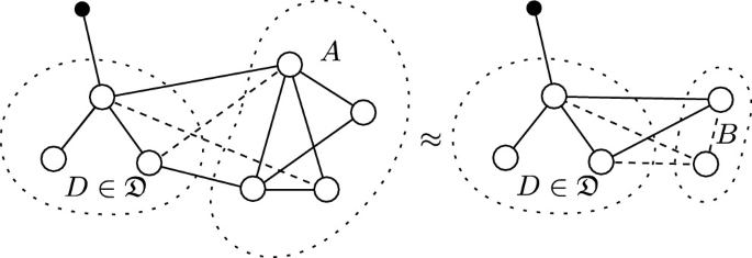
(Composable) simulation-based security proofs are then proofs that there exists an extension to one network connecting only on adversarial interfaces, such that it is observationally indistinguishable to another. We visualise and provide an example of construction in Fig. 2. Please be aware that despite the similar notation and model, the notion of construction described here differs significantly from that used in Constructive Cryptography.⁴

Definition 9

(Network Construction). A network $A \in \mathfrak {N}$ constructs another network $B \in \mathfrak {N}$ with respect to a distinguisher class $\mathfrak {D}$ with simulator $\alpha \in \mathfrak {N}$ and error $\epsilon \in \mathbb {R}$, written , if and only if $A \overset{\epsilon ,\mathfrak {D}}{\sim } \alpha B$ and $\alpha$ and B have disjoint honest interfaces: ${IO}_{\mathcal {H}}(\alpha ) \cap {IO}_{\mathcal {H}}(B) = \varnothing$. The $\mathfrak {D}$ term may be omitted when it is clear from the context, the $\alpha$ term may be omitted when it is of no interest, and the $\epsilon$ term may be omitted when it is negligible.

Fig. 2.

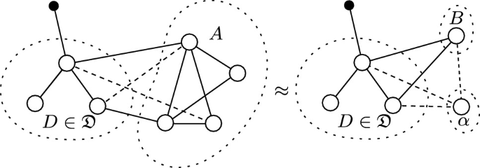
A visual representation of a non-specific experiment.

As with observational indistinguishability, network construction statements can be arbitrarily weakened. Furthermore, it is directly implied by indistinguishability:

(5)

(6)

Theorem 1

(Generalised Composition). Network construction is composable, in that is satisfies transitivity (Eq. 7), subgraph substitutability (Eq. 8), and renameability (Eq. 9). For all $A, B, C, \alpha , \beta \in \mathfrak {N}, \mathfrak {D}\subseteq \mathfrak {N}, \epsilon _1, \epsilon _2 \in \mathbb {R}, \vec {n}$:

(7)

(8)

(9)

Proof

We will prove each of the three properties separately.

Transitivity. By assumption, we know that $A \overset{\epsilon _1,\mathfrak {D}}{\sim } \alpha B$ and $B \overset{\epsilon _2,\mathfrak {D}\alpha }{\sim } \beta C$. By Lemma 3, we can conclude that $\alpha B \overset{\epsilon _2,\mathfrak {D}}{\sim } \alpha \beta C$. By transitivity (Lemma 2), we conclude that $A \overset{\epsilon _1 + \epsilon _2, \mathfrak {D}}{\sim } \alpha \beta C$.

Observe that $\beta$ and C, as well as $\alpha$ and B have disjoint honest interfaces by assumption. As $B \overset{\epsilon _2,\mathfrak {D}}{\sim } \beta C$, they have the same public-facing interfaces. As $\alpha \beta C$ is well-defined, and as $\alpha$ and B have disjoint honest interfaces, so does $\alpha$ and $\beta C$. From each of $\alpha$, $\beta$, and C’s honest interfaces being disjoint, we conclude that so are $\alpha \beta$ and C’s.    $\square$

Closure under subgraph substitution. By assumption, we know $A \overset{\epsilon _1, \mathfrak {D}C}{\sim } \alpha B$. By Lemma 3, we can conclude that $CA \overset{\epsilon _1, \mathfrak {D}}{\sim } C\alpha B$. As composition is a disjoint union, it is commutative, and therefore $C\alpha B = \alpha CB$. The interface disjointness requirement is satisfied by the precondition.    $\square$

Closure under renaming. By assumption, we know $A \overset{\epsilon _1, \mathfrak {D}}{\sim } \alpha B$. By Lemma 1, we conclude that $A[\vec {n}] \overset{\epsilon _1, \mathfrak {D}[\vec {n}]}{\sim } (\alpha B)[\vec {n}] = \alpha [\vec {n}]B[\vec {n}]$. As $\alpha [\vec {n}]B[\vec {n}] \in \mathfrak {N}$, both $\alpha [\vec {n}]$ and $B[\vec {n}]$ are in $\mathfrak {N}$. As the honesty of edges remains unaffected by subgraph substitution, name collisions are not introduced, the disjointness requirement is also satisfied. Combined, this implies network construction in the renamed setting.    $\square$

From the generalised composition theorem, which notably relies on modifying the distinguisher set (e.g. from $\mathfrak {D}$ to $\mathfrak {D}\alpha$ in Eq. 7), we can infer operations similar to sequential and parallel composition in Constructive Cryptography, given $\mathfrak {D}= \mathfrak {N}$. For any $\mathfrak {D}$, identity also holds, due to the identity of indistinguishability, and indistinguishability lifting to construction.

Corollary 2

(Traditional Composition). For $\mathfrak {D}= \mathfrak {N}$, honest network construction has the following, simpler statements for universal transitivity (Eq. 10) and universal closure under subgraph substitution (Eq. 11). Identity (Eq. 12) holds regardless of $\mathfrak {D}$. For all $A, B, C, \alpha , \beta \in \mathfrak {N}, \epsilon _1, \epsilon _2 \in \mathbb {R}, \mathfrak {D}\subseteq \mathfrak {N}$:

(10)

(11)

(12)

4 The Limited Composition of ${\mathfrak {K}}$-Networks

Having established a composition system which allows restricting the domain of permissible distinguishers, and having formalised the general notion of knowledge assumptions, we can now establish the main contribution of this paper: Permitting extraction from knowledge assumptions within a composable setting.

We use a similar idea to that of “algebraic adversaries” in the Algebraic Group Model [17], requiring random systems to output not only knowledge-implying objects, but also their corresponding witness. We then add new nodes to the network which gather all data extracted in this way in a central repository of knowledge for each knowledge assumption. Crucially, while the distinguisher supplies witnesses for all knowledge-implying objects it outputs, it is not capable of retrieving witnesses from other parts of the system.

Simulators are provided with read access to this repository, allowing the simulator to extract the knowledge it requires, but not any more about the behaviour of honest parties. The composition of constructions using knowledge assumptions is proven, provided the parts being composed do not both utilise the same knowledge assumption. In such a case, Theorem 1 provides a fall-back for what needs to be proven, namely that the simulator of one system does not permit distinguishing in the other system. At a technical level, modifications to Definition 3 are needed to allow types to depend on previously transmitted values. We note these formally in the full version of this paper [24, Appendix C]. This section serves as a detailed proof sketch, with [24, Appendix C] addressing some of the subtleties.

4.1 Knowledge Respecting Systems

The Algebraic Group Model [17] popularised the idea of “algebraic” adversaries, which must adhere to outputting group elements through a representation describing how they may be constructed from input group elements. Security proofs in the AGM assume that all adversaries are algebraic, and therefore the representation of group elements can be directly accessed in the reduction – by assumption it is provided by the adversary itself.

While this is equivalent to an extractor-based approach, for composition we will follow a similar “algebraic” approach. The premise is that for any random system R outputting (among other things) knowledge-implying objects in ${\mathfrak {K}}$, it is possible to construct an equivalent random system ${\mathfrak {K}}(R)$, which outputs the corresponding witnesses as well, provided each step of the random system is governed by a ${\mathfrak {K}}$-respecting algorithm.

Recall that a random system is an infinite sequence of probability distributions. As this is not in itself useful for applying Definition 1, we instead interpret them as an equivalence class over stateful, interactive, and probabilistic algorithms [29], with associated input and output types. For any such typed algorithm A and knowledge assumption ${\mathfrak {K}_\mathsf {pp}}$, A can be separated into $A_1$ and $A_2$, where $A_1$ outputs only a series of $[X_\mathsf {pp}]$ values, and $A_2$ all the remaining information, such that A’s output can be trivially reconstructed by inserting the $[X_\mathsf {pp}]$ values of $A_1$ into the gaps in $A_2$’s outputs. Likewise, inputs can be split into the $\vec {I}$ and $\mathsf {aux}$ inputs used in Game 1. Given this, we can define when a random system is ${\mathfrak {K}}$-respecting. Each such system has a corresponding “${\mathfrak {K}}$-lifted” system, which behaves “algebraically”, in that it also output witnesses.

Definition 10

(${\mathfrak {K}}$-Respecting Systems). A typed random system R is said to be ${\mathfrak {K}}$-respecting (or $R \in \mathsf {RespSys}_{\mathfrak {K}}$), if and only if its equivalence class of stateful probabilistic algorithms contains a stateful algorithm A that when split as described in Subsect. 4.1 into $A_1$ and $A_2$, satisfies $A_1 \in \mathsf {Resp}_{\mathfrak {K}}$. For a set ${\vec {\mathfrak {K}}}$, $\mathsf {RespSys}_{\vec {\mathfrak {K}}}:=\bigcap _{{\mathfrak {K}}\in {\vec {\mathfrak {K}}}} \mathsf {RespSys}_{\mathfrak {K}}$.

Definition 11

(${\vec {\mathfrak {K}}}$-Lifted Systems). A typed random system R induces a set of ${\vec {\mathfrak {K}}}$-lifted random systems. This is defined by replacing, for any ${\mathfrak {K}}= (\cdot , X, W, \mathcal {R}) \in {\vec {\mathfrak {K}}}$, any (part of) an output from R with type $[{\mathfrak {K}_\mathsf {pp}}]$ with (a part of) the output with type $\langle {\mathfrak {K}_\mathsf {pp}}, I_{\mathfrak {K}_\mathsf {pp}}\rangle$, where $I_{\mathfrak {K}_\mathsf {pp}}$ is constructed as the set of all prior inputs to R of type $[{\mathfrak {K}_\mathsf {pp}}]$. The output (part) $\langle x, w \rangle _{\mathfrak {K}_\mathsf {pp}}^{I_{\mathfrak {K}_\mathsf {pp}}}$ of the lifted system must be such that the equivalent output (part) on the unlifted system is $[x]_{\mathfrak {K}_\mathsf {pp}}$, and $(x, w) \in \mathcal {R}_{\mathfrak {K}_\mathsf {pp}}(I_{\mathfrak {K}_\mathsf {pp}})$ with overwhelming probability.

Theorem 2

(${\vec {\mathfrak {K}}}$-Lifting is Possible). For random systems $R \in \mathsf {RespSys}_{\vec {\mathfrak {K}}}$, at least one ${\vec {\mathfrak {K}}}$-lifting of R, denoted ${\vec {\mathfrak {K}}}(R)$, exists.

Proof

Split R into algorithms $A_{\mathfrak {K}}$ for each ${\mathfrak {K}}\in {\vec {\mathfrak {K}}}$, and $A_*$ for the remaining computation, such that each $A_{\mathfrak {K}}$ outputs only $[{\mathfrak {K}}]$, and $A_*$ outputs no such values, as described above. Then, by Assumption 1, there exist corresponding extractors $\mathcal {X}_{\mathfrak {K}}$ for each ${\mathfrak {K}}\in {\vec {\mathfrak {K}}}$, such that given the same inputs $\mathcal {X}_{\mathfrak {K}}$ outputs witnesses to the knowledge-implying objects output by $A_{\mathfrak {K}}$.

Replace $A_{\mathfrak {K}}$ with $A'_{\mathfrak {K}}$, which runs both $A_{\mathfrak {K}}$ and $\mathcal {X}_{\mathfrak {K}}$, and outputs $\langle x, w \rangle _{\mathfrak {K}}$, where $[x]_{\mathfrak {K}}$ is the output of $A_{\mathfrak {K}}$, and w is the output of $\mathcal {X}_{\mathfrak {K}}$. When reassembled into a random system, this modification satisfies Definition 11.    $\square$

4.2 Lifting Networks for Knowledge Extraction

The set of ${\vec {\mathfrak {K}}}$-respecting random systems $\mathsf {RespSys}_{\vec {\mathfrak {K}}}$, along with the transformation ${\vec {\mathfrak {K}}}(R)$ for any $R \in \mathsf {RespSys}_{\vec {\mathfrak {K}}}$, provides a means of lifting individual random systems. Applied to networks, it is clear something more is necessary – the lifting does not preserve the types of output interfaces, and to permit these to match again some additional changes need to be made to the networks. Looking forward, the lifted systems will interact with a separate, universal node $\textsc {repo}$, which stores witnesses for the simulator to access.

We extend the notion of ${\vec {\mathfrak {K}}}$-respecting to apply to networks, a network is ${\vec {\mathfrak {K}}}$-respecting if and only if all vertices in it are also ${\vec {\mathfrak {K}}}$-respecting (we will use $\mathsf {RespNet}_{\vec {\mathfrak {K}}}$ as the corresponding set of ${\vec {\mathfrak {K}}}$-respecting networks⁵). In lifting networks in this set, not only is each individual node lifted, but all outgoing connections are connected to a new node, which we name $\textsc {Charon}$, which acts as a relay; re-erasing witnesses, while also informing a central repository of knowledge (outside of this network) of any witnesses it processes. We take the name from the ferryman of the dead in ancient Greek mythology, who in our case demands his toll in knowledge rather than coins. For any ${\vec {\mathfrak {K}}}$-respecting network N, we define the lifting ${\vec {\mathfrak {K}}}(N)$ as follows:

Definition 12

(Network Lifting). The network lifting ${\vec {\mathfrak {K}}}(N)$ for any cryptographic network $N \in \mathsf {RespNet}_{\vec {\mathfrak {K}}}$ is defined to compose as expected. In particular, if there exists ${\vec {\mathfrak {K}}}', N' : N = {\vec {\mathfrak {K}}}'(N')$, then ${\vec {\mathfrak {K}}}(N)$ is defined as $({\vec {\mathfrak {K}}}\cup {\vec {\mathfrak {K}}}')(N')$. Otherwise⁶, ${\vec {\mathfrak {K}}}(N)$ is defined as consisting of nodes $n'$ for each node $n \in N$, where $R_{n'} = {\vec {\mathfrak {K}}}(R_n)$, and each output interface is renamed to a unique⁷ new interface name. For each output interface now named x, and previously named y in N, ${\vec {\mathfrak {K}}}(N)$ contains a new node $\textsc {Charon}({\vec {\mathfrak {K}}}, \mathsf {adv})$, where $\mathsf {adv}$ denotes if the interface is adversarial, connected to free interfaces on the knowledge repository $\textsc {repo}$ and the public parameters for each knowledge assumption. Note that $\textsc {repo}$ is not part of the lifted network itself, which allows disjoint networks to remain disjoint when lifted.

We specify the node $\textsc {Charon}$ in full detail in [24, Appendix B], along with the node $\textsc {repo}({\mathfrak {K}})$, which collects witnesses from $\textsc {Charon}$, and provides adversarial access to them. $\textsc {repo}$ allows for some variation. For instance, it could

• 1. Return the set of all witnesses.

• 2. Return at most one witness.

• 3. Abort when no witness is available.

• 4. For recursive witnesses (such as those used in the AGM and KEA assumptions), consolidate the witness into a maximal one, by recursively resolving $(\textsc {input}, i)$ terms.

We focus on 1, as it is the simplest. The set of valid ${\vec {\mathfrak {K}}}$-distinguishers $\mathfrak {D}_{\vec {\mathfrak {K}}}$ is defined with respect to $\textsc {repo}$, where we assume the choice of variation is made separately for each knowledge assumption. Informally, it ensures that all parts of the distinguisher are ${\vec {\mathfrak {K}}}$-lifted, and the distinguisher collects all witnesses in a central knowledge repository $\textsc {repo}$, but does not retrieve witnesses from this, effectively only providing access to the simulator.

Definition 13

(${\vec {\mathfrak {K}}}$-Distinguishers). The set of valid ${\vec {\mathfrak {K}}}$-distinguishers $\mathfrak {D}_{\vec {\mathfrak {K}}}$, for any set of knowledge assumptions ${\vec {\mathfrak {K}}}$, is defined as the closure under internal renaming of

Note that as $N \in \mathsf {RespNet}_{\vec {\mathfrak {K}}}$, it cannot directly connect to any of the $\textsc {repo}$ nodes.

As the number of $\textsc {repo}$ and public parameter interfaces may differ between the real and ideal world, we must normalise them before establishing indistinguishability. To do so, we wrap both worlds to contain an additional node, which we name $\bot$, which consumes all remaining interfaces, depending on the number already used. Formally, this is defined in [24, Appendix B.3].

Given these definitions, existing indistinguishability and construction results between ${\vec {\mathfrak {K}}}$-respecting networks can be lifted to equivalent results between the lifted networks, with respect to ${\vec {\mathfrak {K}}}$-distinguishers:

Lemma 4

(Indistinguishability Lifting). If $A_1A_2 \overset{\epsilon , \mathfrak {D}_{{\vec {\mathfrak {K}}}_1}}{\sim } B_1B_2$, where for $i\in \{1,2\}$, $A_i, B_i \in \mathsf {RespNet}_{{\vec {\mathfrak {K}}}_2}$, ${\vec {\mathfrak {K}}}_1 \cap {\vec {\mathfrak {K}}}_2 = \varnothing$, and ${\vec {\mathfrak {K}}}:={\vec {\mathfrak {K}}}_1 \cup {\vec {\mathfrak {K}}}_2$, then:

$$\begin{aligned} A_1A_2 \overset{\epsilon ,\mathfrak {D}_{{\vec {\mathfrak {K}}}_1}}{\sim } B_1B_2 \implies A_1{\vec {\mathfrak {K}}}_2(A_2) \overset{\epsilon ,\mathfrak {D}_{\vec {\mathfrak {K}}}}{\sim } B_1{\vec {\mathfrak {K}}}_2(B_2). \end{aligned}$$

Lemma 5

(Construction Lifting). For $A_{1,2}, B_{1,2}, \alpha _{1,2} \in \mathsf {RespNet}_{{\vec {\mathfrak {K}}}_2}$ and ${\vec {\mathfrak {K}}}_1, {\vec {\mathfrak {K}}}_2$ where ${\vec {\mathfrak {K}}}_1 \cap {\vec {\mathfrak {K}}}_2 = \varnothing$, and ${\vec {\mathfrak {K}}}:={\vec {\mathfrak {K}}}_1 \cup {\vec {\mathfrak {K}}}_2$:

We visualise the construction experiment against a knowledge-respecting distinguisher set $\mathfrak {D}_{\mathfrak {K}}$ in Fig. 3. This may be contrasted with Fig. 2, which does not have $\textsc {repo}({\mathfrak {K}})$, and does not allow the simulator to extract.

Fig. 3.

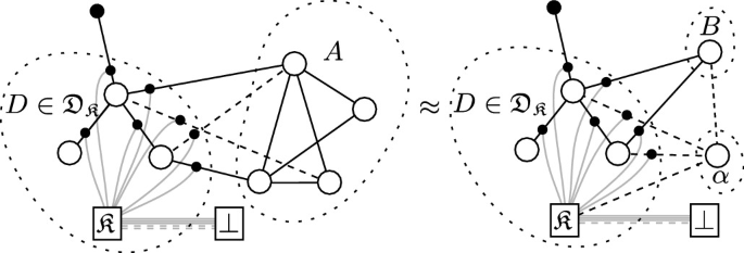
A visual representation of a non-specific experiment. The small points denote $\textsc {Charon}({\mathfrak {K}})$ nodes, while ${\mathfrak {K}}$ denotes the $\textsc {repo}({\mathfrak {K}})$ node. Public parameters have been omitted. Note that outside of $D$ $\textsc {Charon}$ nodes are permitted, but not required.

Lemma 6

($\mathfrak {D}_{\vec {\mathfrak {K}}}$ Closure).$\mathfrak {D}_{{\vec {\mathfrak {K}}}}$ is closed under sequential composition with lifted (with respect to ${\vec {\mathfrak {K}}}$) networks in $\mathsf {RespNet}_{{\vec {\mathfrak {K}}}}$: $\forall R \in \mathsf {RespNet}_{{\vec {\mathfrak {K}}}} : \mathfrak {D}_{{\vec {\mathfrak {K}}}}{\vec {\mathfrak {K}}}(R) \subseteq \mathfrak {D}_{{\vec {\mathfrak {K}}}}$

Proof

Follows immediately from $\mathsf {RespNet}_{{\vec {\mathfrak {K}}}}$ being closed under set union, and Definition 13 stating that any ${\vec {\mathfrak {K}}}$-lifted network has a corresponding distinguisher in $\mathfrak {D}_{\vec {\mathfrak {K}}}$.    $\square$

As a stricter set of knowledge assumptions corresponds to a smaller set of permissible distinguishers, indistinguishability and construction results can be transferred to larger sets of knowledge assumptions. A proof without knowledge assumptions is clearly ideal – it still holds, regardless which knowledge assumptions are added.

Lemma 7

(Knowledge Weakening). In addition to weakening with respect to a subset of distinguishers being possible, weakening is also possible for distinguishers with a greater set of knowledge assumptions. For all $A, B, C, \alpha \in \mathfrak {N}, {\vec {\mathfrak {K}}}_1, {\vec {\mathfrak {K}}}_2$, where ${\vec {\mathfrak {K}}}_1 \subseteq {\vec {\mathfrak {K}}}_2$:

(13)

(14)

4.3 A Restricted Composition Theorem

The rules established in Theorem 1 still hold, and it is clear why a simplification as in Corollary 2 is not possible – it assumes that the distinguisher set $\mathfrak {D}$ is closed under sequential composition with simulators and networks, which is not the case for $\mathfrak {D}_{\vec {\mathfrak {K}}}$.

Theorem 1 already provides a sufficient condition for what needs to be proven to enable this composition, however we can go a step further: While $\mathfrak {D}_{\vec {\mathfrak {K}}}$ is not closed under sequential composition with arbitrary networks, it is closed under sequential composition with knowledge-lifted networks. We can use this fact to establish a simplified composition theorem when composing with a ${\vec {\mathfrak {K}}}$-lifted proof or network component. We observe that this implies composition with proofs which do not utilise knowledge assumptions, as they are isomorphic to ${\vec {\mathfrak {K}}}= \varnothing$. In particular, Constructive Cryptography proofs directly imply construction in the context of this paper as well, and can therefore be composed with protocols utilising our framework freely.

Theorem 3

(Knowledge Composition). When composing proofs against ${\vec {\mathfrak {K}}}_1$ or ${\vec {\mathfrak {K}}}_2$ distinguishers, where ${\vec {\mathfrak {K}}}_1 \cap {\vec {\mathfrak {K}}}_2 = \varnothing$, and ${\vec {\mathfrak {K}}}:={\vec {\mathfrak {K}}}_1 \cup {\vec {\mathfrak {K}}}_2$, the following simplified composition rules of transitivity (Eq. 15) and subgraph substitution (Eq. 16) apply. For all $A, B, \alpha \in \mathsf {RespNet}_{{\vec {\mathfrak {K}}}_2}, F \in \mathsf {RespNet}_{{\vec {\mathfrak {K}}}}, C, D, E, \beta , \gamma \in \mathfrak {N}, \epsilon , \epsilon _1, \epsilon _2$.

(15)

(16)

4.4 Reusing Knowledge Assumptions

Theorem 3 and its supporting lemmas prominently require disjoint sets of knowledge assumptions. The primary reason for this lies in the definition of ${\vec {\mathfrak {K}}}$ using the union of the knowledge assumptions ${\vec {\mathfrak {K}}}_1$ and ${\vec {\mathfrak {K}}}_2$ – all statements could also be made using a disjoint union here instead. If knowledge assumptions were not disjoint, this would place an unreasonable constraint on the distinguisher however: It would prevent it from copying information from one instance of a knowledge assumption to another instance of the same knowledge assumption, something any adversary is clearly capable of doing.

Equality for knowledge assumptions is not really well defined, and indeed knowledge assumptions may be related. The disjointness requirement is therefore more a statement of intent than an actual constraint, and we stress the importance of it for reasonably constraining the distinguisher set here: If the distinguisher is constrained with respect to two instances of knowledge assumptions which are related, it may not be permitted to copy from one two to another for instance, an artificial and unreasonable constraint.

Care must be taken that knowledge stemming from one knowledge assumption does not give an advantage in another. In many – but not all – cases this is easy to establish, for instance, we conjecture that multiple instances with the AGM with independently sampled groups are sufficiently independent. If this care is not taken, the union of two knowledge assumptions may be greater than the sum of its parts, as using both together prevents the distinguisher from exploiting structural relationships between the two, something a real adversary may do.

5 zk-SNARKs with an Updateable Reference String

To demonstrate the usefulness of this framework, we will showcase an example of how it can lift existing results to composability. For brevity, we sketch the approach instead of providing it in full detail. Specifically, we sketch how Groth’s zk-SNARK [20], due to being simulation extractable [1], can be used to construct an ideal NIZK. Our methodology applies to any SNARK scheme which permits proof simulation and extraction through the AGM. Further, we sketch how, when used for a SNARK requiring an updateable reference string, a round-robin protocol to produce the reference string can be used to instantiate the NIZK from only the CRS providing the AGM parameters.

Our approach for NIZKs is similar to C$\emptyset$C$\emptyset$ [28], with the difference that no additional transformation is necessary to extract witnesses, as these are provided through ${\mathfrak {K}}_\mathsf {bAGM}$-lifting and the simulator’s ability to extract from the knowledge assumption. The round-robin update follows [25] for its composable treatment updateable reference strings, simplified to a setting with fixes participants.

Once our proof sketch is complete, we also give a clear example of why universal composition is not possible with knowledge assumptions: Specifically, we construct a complementary ideal network and simulator which clearly violates the zero-knowledge properties of the NIZK, and allows distinguishing the real and ideal worlds. We stress that this is only possible due to it extracting from the same knowledge assumption.

5.1 Construction

Our construction is in two parts, each consisting of a real and ideal world. We describe and illustrate the set-up and behaviour here, leaving a more formal description of the exact behaviour to the full version of this paper [24, Appendix D]. Throughout the construction, we assume a set of n parties, identified by an element in $\mathbb {Z}_n$. We assume static corruption with at least one honest party – specifically we assume a set of adversaries $\mathcal {A}\subset \mathbb {Z}_n$, and a corresponding set of honest parties ${\mathcal {H}}:=\mathbb {Z}_n \setminus \mathcal {A}$. These sets cannot be used in the protocols themselves, but are known to the distinguisher and non-protocol nodes (that is, they can be used to define ideal behaviour).

SNARKs. The highest level ideal world consists of a proof-malleable NIZK node (nizk, see [24, Appendix D.2]), following the design of C$\emptyset$C$\emptyset$ [28]. In the corresponding real-world, we use a zk-SNARK scheme $\mathcal {S} = (S, T, P, \mathsf {Prove}, \mathsf {Verify},\mathsf {SimProve}, \mathcal {X}_w)$ satisfying the standard properties of correctness, soundness, and zero-knowledge in the random oracle model with SRS. Here S, T, and P, are the structure function, trapdoor domain, and permissible permutations⁸ of the structured reference strings, as given in [25]. $\mathsf {SimProve}$ should take as inputs only the statement x and trapdoor $\tau \in T$. In addition, $\mathcal {S}$ should be simulation extractable with respect to the AGM – after any arbitrary interaction, $\mathcal {X}_w$ should be able to produce the witness for any valid statement/proof pair, with the sole exception that the proof was generated with $\mathsf {SimProve}$. Such white-box simulation extractability has been under-studied for zk-SNARKs, although it has been established for Groth’s zk-SNARK [1], and is plausible to hold in the AGM for most SNARKs. For this reason, we rely on Groth’s zk-SNARK to concretely instantiate this example, although we conjecture it applies to other SNARKs – and indeed part of the result can only apply to other SNARKs.

In the real world an adversarially biased (updateable) structured reference string (srs, see [24, Appendix D.3]), parameterised for the SNARK’s reference string, is available. Further, for each honest party $j \in {\mathcal {H}}$, an instance of the SNARK protocol node (snark-node(j), see [24, Appendix D.3]) is available, which connects to the corresponding party’s srs interface, and runs the SNARK’s $\mathsf {Prove}$ and $\mathsf {Verify}$ algorithms when queried. In both worlds, the ${\mathfrak {K}}_\mathsf {bAGM}$ public parameters are provided by a node $\mathbb {G}$ (see [24, Appendix D.1]). Finally, the SNARK’s $\mathsf {Prove}$ and $\mathsf {Verify}$ algorithms make use of a random oracle, which is available in the real world, providing query interfaces to all parties (we do not treat the random oracle as a knowledge assumption in this example).

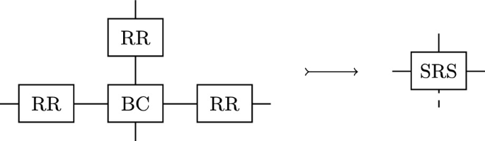
The ideal-world therefore consists of $\{\textsc {nizk}, \mathbb {G}\}$ (and the simulator, which will be introduced in the security analysis), and the real-world consists of $\textsc {snark} \uplus \{\textsc {srs}, \textsc {ro}, \mathbb {G}\}$, where $\textsc {snark} :=\{\;\textsc {snark-node}(j) \mid j \in {\mathcal {H}}\;\}$. The topology of both worlds is sketched in Fig. 4.

Fig. 4.

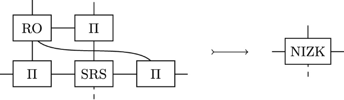
The SNARK to NIZK topologies. snark-node is represented by $\mathrm {\Pi }$, and the public parameter node $\mathbb {G}$ is omitted for clarity.

Round-robin SRS. If the reference string used in the SNARK scheme $\mathcal {S}$ is also updateable in the sense of [25], we can construct the SRS itself through a round-robin update protocol. We assume therefore that $\mathcal {S}$ is additionally parameterised by algorithms $\mathsf {ProveUpd}$ and $\mathsf {VerifyUpd}$ allowing the proving and verification of update proofs, the permutation lifting $\dagger$ which maps permutations in P to permutations over the structure, and the algorithms $\mathcal {S}_\rho$ and $\mathcal {X}_p$ used by the simulator to simulate update proofs and extract permutations from updates respectively. A notable difference again with respect to the extraction is that it should be with respect to the AGM, rather than with respect to a NIZK as presented in [25].

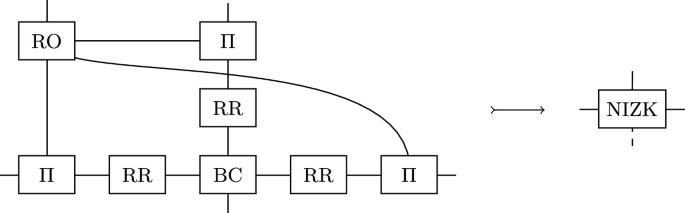
The ideal world in this part matches part of the SNARK real world previously, consisting of the pair of nodes $\{\textsc {srs}, \mathbb {G}\}$. The real-world consists of a node providing synchronous, authenticated broadcast (bcast, see [24, Appendix D.4]), and for each honest party $j \in {\mathcal {H}}$, a round-robin protocol node (rr-node(j), see [24, Appendix D.4]).

The srs node requires each honest party to request initialisation, which in the round-robin node is mapped to a) reconstructing the current SRS, and b) broadcasting a randomly sampled update to it. As the real-world has no means of identifying honest parties, it requires all parties to broadcast a valid update before the reference string can be used. The adversary has access to the broadcast directly for corrupted parties to produce these updates.

The ideal-world therefore consists of $\{\textsc {srs}, \mathbb {G}\}$ (and simulator), and the real-world consists of $\textsc {rr-setup} \uplus \{\textsc {bcast}, \mathbb {G}\}$, where $\textsc {rr-setup} :=\{\;\textsc {rr-node}(j) \mid j \in {\mathcal {H}}\;\}$. The topology of both worlds is sketched in Fig. 5.

Fig. 5.

The round-robin setup to SRS topologies. bcast and rr-node are abbreviated to bc and rr respectively, and the public parameter node $\mathbb {G}$ is omitted for clarity.

5.2 Security Analysis

This example is interesting for two reasons: Firstly, it provides a concrete way to realise a composable NIZK, and secondly it showcases (when the second optional stage of realising the SRS is used) special-case composition between two constructions using the same knowledge assumption, and what this requires of the corresponding simulators, as both simulators extract from $\textsc {repo}({\mathfrak {K}}_\mathsf {bAGM})$.

The two simulators, $\alpha$ for the simulator between snark and nizk, and $\beta$ for the simulator between rr-setup and srs, are specified in full detail in the full version of this paper [24, Appendix D.5], although we sketch the most important aspects here. Notably, $\alpha$ needs to extract the witnesses from adversarial SNARK proofs, and $\beta$ needs to extract the underlying trapdoor permutation from adversarial updates.

Round-robin SRS. The simulator $\beta$ for the round-robin SRS setup emulates the broadcast node bcast towards the adversary, and when notified of an honest party’s initialisation, does one of two things: For the first honest party, it queries the honest SRS part from srs, and simulates the corresponding update proof using the simulator $\mathcal {S}_\rho$, as it knows the full trapdoor to use for this. For subsequent honest updates, it simply simulates the update protocol. In either case, the update is internally recorded to emulate the corresponding broadcast.

When an adversarial broadcast is received, the update is verified against the current SRS. If it succeeds, it is updated, and the corresponding permutation is extracted from the update proof (using ${\mathfrak {K}}_\mathsf {bAGM}$), and recorded. Specifically, the extractor $\mathcal {X}_p$, given oracle access to $\textsc {repo}({\mathfrak {K}}_\mathsf {bAGM})$, extracts the permutation from any update proof $\rho$. Observe that a) such a permutation exists by the nature of the verification of update proofs, and b) the only group elements which the simulator cannot extract from are those in the honest SRS component produced by the srs node.

Given this, the adversary cannot create a valid update for which the permutation is not extractable, unless it reuses (part of) the honest update. This would directly require inverting its structure before re-applying (part of) it again however, or the adversary extracting the permutation itself. In either case, this amounts to breaking a discrete logarithm for SNARKs we considered, which we assume computationally infeasible.

Theorem 4

(Round-Robin uSRS). Given the computational hardness of the structure function S, as well as computational hardness to extract a trapdoor permutation p from an update proof $\rho$:

Proof

(sketch). The simulated broadcast network the adversary has access to behaves identically between the real protocol and the simulated one, due to identical execution, except for the first honest update. This is distributed uniformly randomly in the space of possible permutations in both cases.

As the simulator reproduces a permutation which applies precisely all updates after the first honest one, and the first honest update is distributed the same in both worlds, the permutation the simulator applies to the honest trapdoor causes it to be distributed as in the real protocol. Further, both worlds abort if and only if the reference string is queried prior to full initialisation in both worlds. By the reasoning above and the hardness assumptions, extraction of adversarial updates always succeeds, and as a result the simulated update proof also succeeds.    $\square$

SNARK. The SNARK simulator $\alpha$ both faithfully simulates the srs node, creates simulated proofs for honest proving queries, and extracts witnesses using $\mathcal {X}_w$ (which is given access to $\textsc {repo}({\mathfrak {K}}_\mathsf {bAGM})$) from adversarial proofs when requested by the nizk node. Finally, if the simulator fails to extract a witness when asked for one for a valid proof, it requests a maul. The SNARK simulator can co-exist with the SRS simulator provided above, provided that the SRS update proofs cannot be interpreted as NIZK proofs (with the trapdoor permutation as a witness) themselves, or transformed into ones. In practice, this is not the case, as the AGM allows only for very specific transformations of group elements, and mapping update proofs to a corresponding NIZK would involve first solving DLOG before re-encoding the witness as a polynomial in most SNARKs.

Theorem 5

(SNARK Protocols Construct NIZKs). For any secure SNARK scheme $\mathcal {S}$:

(17)

Additionally, if $\mathcal {S}$ is updateable (and therefore $\beta$ is well-defined), and update proofs cannot be transformed into NIZK proofs with the trapdoor permutation as a witness:

(18)

Proof

(sketch). All honestly generated proofs will verify in both worlds, by definition in the ideal world, and by the correctness of the SNARK in the real world. Further, the proofs themselves are indistinguishable, by the zero-knowledge property of the SNARK.

Adversarial proofs which fail to verify will also be rejected in the ideal world, as the simulator will refuse to provide a witness, causing them to be rejected. As per the above, the extractor $\mathcal {X}_w$ is able to (using $\textsc {repo}({\mathfrak {K}}_\mathsf {bAGM})$) extract the witnesses for any adversarial proof which does verify, except for cases of malleability. As $\mathcal {S}$ is only (at most) proof-malleable, the simulator can, and does, account for this by attempting to create a mauled proof when extraction fails.

The simulator provides the ideal-world simulation of the srs node, which is emulated faithfully except that the simulator has access to the trapdoor. As a result, this part of the system cannot be used to distinguish. We conclude that Eq. 17 holds.

For Eq. 18, it remains to be shown that $\alpha$ and $\beta$ do not interfere: In particular, that neither prevents the other from extracting where they need to, and that neither reveal information due to their extractions which would provide the distinguisher a non-negligible advantage. As $\beta$ only interacts with the SRS, and this is not changed once all users have submitted their contribution, and $\alpha$ requires the SRS to be fully initialised before it is used, $\alpha$ will not prevent $\beta$ from extracting – it does nothing while $\beta$ is run.

Knowledge of the group elements exchanged during the update phase also does not assist the distinguisher in constructing a witness for any statement, as it can simulate them locally by running the honest update process. Therefore $\alpha$ can still fully extract in all cases.

Finally, due to the strict temporal order, $\beta$ can, by definition, not assist the distinguisher in extracting any additional differences between snark and $\alpha$ (and the srs part is emulated faithfully, preventing it there). Likewise, $\alpha$ cannot assist the distinguisher in extracting anything meaningful from $\beta$, as this would imply a NIZK witness containing the permutation of an honest update. As these are sampled locally, and the corresponding update proofs cannot be transformed into NIZK proofs, $\alpha$ cannot be leveraged to extract them.    $\square$

Corollary 3

For an updateable SNARK scheme $\mathcal {S}$ whose update proofs cannot be transformed into NIZK proofs with the trapdoor permutation as a witness:

The topology for the composed statement arises naturally from the topologies of its parts, as shown in Fig. 6.

Fig. 6.

The combined full example topology, arising from the composition of prior components, again with $\mathbb {G}$ omitted for clarity.

Proof

From Theorem 4, Theorem 3 and Eq. 16, we can conclude that . The corollary then follows from Theorem 5, Theorem 3, Eq. 18 and Eq. 15.    $\square$

5.3 The Impossibility of General Composition

The two parts of Theorem 3 are limited when compared to Corollary 2 in two separate, but related ways: The closure under subgraph substitution requires the added node to be a ${\vec {\mathfrak {K}}}$-wrapped node, and transitivity requires the two composing proofs to use separate knowledge assumptions.

We will demonstrate that the nicer results from Corollary 2 are not achievable with respect to knowledge-respecting distinguishers, by means of a small counter-example for both situations.

Theorem 6

(Subgraph Substitution is Limited). Subgraph substitution with knowledge assumptions does not universally preserve secure construction. $\exists A, B, C, \alpha \in \mathfrak {N}, \epsilon \in \mathbb {R}, {\vec {\mathfrak {K}}}$:

Proof

(sketch). Let A be the Groth-16 real world, and B be the NIZK ideal world respectively, with $\alpha$ being their simulator, and ${\vec {\mathfrak {K}}}$ being $\{{\mathfrak {K}}_\mathsf {bAGM}\}$. Let C be a node which receives elements in $X_\mathsf {pp}$, queries $\textsc {repo}({\mathfrak {K}}_\mathsf {bAGM})$, and returns the witness to the distinguisher.

Then the following distinguisher can trivially distinguish the two worlds: a) Make any honest proving query. b) Request extraction. c) Output whether or not extraction succeeded.    $\square$

Theorem 7

(Transitivity is Limited). Construction with knowledge assumptions is not universally transitive. $\exists A, B, C, \alpha , \beta \in \mathfrak {N}, \epsilon _1, \epsilon _2 \in \mathbb {R}, \mathfrak {D}_{\vec {\mathfrak {K}}}$:

Proof

(sketch). Let B be the Groth-16 real world, and C be the NIZK ideal world respectively, with $\beta$ being their simulator, and ${\vec {\mathfrak {K}}}$ being $\{{\mathfrak {K}}_\mathsf {bAGM}\}$. Let A be Groth-16 with additional interfaces for each party to reveal any witnesses of broadcast proofs, which are shared through an additional broadcast channel. Let $\alpha$ reproduce this functionality by extracting witnesses from the provided proofs.

Then a distinguisher which makes an honest proof and extracts it will receive the witness in the real and hybrid world, but not in the ideal world, where the knowledge extraction of the proof will fail, as it is simulated by $\beta$. It is therefore possible to distinguish, and transitivity does not hold.    $\square$

6 Conclusion

In this paper, we have for the first time demonstrated the composability of a white-box extractable zk-SNARK, without any transformations or modifications applied, and not compromising on succinctness. This result has immediate applications in the many systems which use zk-SNARKs and non-interactive zero-knowledge, reducing the gap between the theory and practice of composable systems relying on SNARKs. Our results are sufficiently general to hope for similar benefits when applied to other primitives utilising knowledge assumptions.

We nonetheless leave a number of pressing issues to future work: In many cases knowledge assumptions are reused. For instance many different protocols rely on the same groups, with the BLS12-381 and BN-254 curves being de-facto standards for zk-SNARK computation due to their direct use in major software implementations [3, 5]. To what degree this reuse it harmful, if at all, is a question of immediate interest and concern. This is compounded by a recent interest in recursive zk-SNARKs, such as Halo [6] – a natural compositional definition of which would construct a zk-SNARK from itself repeatedly. We hope that this work paves the way for a proper compositional treatment of such recursive constructions.

The foundations of knowledge assumptions also require further fleshing out to match reality more fully. It is clear that some knowledge assumptions are related, for instance the knowledge of exponent assumption is implied by the AGM. More interestingly, non-interactive zero-knowledge can itself be seen as a knowledge assumption – knowledge of a valid proof implying knowledge of the witness. Exploring the formal relationship between different knowledge assumptions and expanding the model to fit these (for instance, by permitting public parameters to be adversarially influenced) may give valuable insight into the nature of these assumptions.

References

Baghery, K., Kohlweiss, M., Siim, J., Volkhov, M.: Another look at extraction and randomization of Groth’s zk-SNARK. In: FC 2021, March 2021
Ben-Sasson, E., et al.: Zerocash: decentralized anonymous payments from bitcoin. In: 2014 IEEE Symposium on Security and Privacy, pp. 459–474. IEEE Computer Society Press, May 2014
Ben-Sasson, E., et al.: libsnark: a C++ library for zkSNARK proofs (2017). https://github.com/scipr-lab/libsnark
Bitansky, N., Canetti, R., Chiesa, A., Tromer, E.: From extractable collision resistance to succinct non-interactive arguments of knowledge, and back again. In: Goldwasser, A. (ed.) ITCS 2012, pp. 326–349. ACM, January 2012
Bowe, S.: bellman (2018). https://github.com/zkcrypto/bellman
Bowe, S., Grigg, J., Hopwood, D: Halo: recursive proof composition without a trusted setup. Cryptology ePrint Archive, Report 2019/1021 (2019). https://eprint.iacr.org/2019/1021
Boyle, E., Pass, R.: Limits of extractability assumptions with distributional auxiliary input. In: Iwata, T., Cheon, J.H. (eds.) ASIACRYPT 2015, Part II. LNCS, vol. 9453, pp. 236–261. Springer, Heidelberg (2015). https://doi.org/10.1007/978-3-662-48800-3_10
Canetti, R.: Universally composable security: a new paradigm for cryptographic protocols. In: 42nd FOCS, pp. 136–145. IEEE Computer Society Press, October 2001
Canetti, R., Dakdouk, R.R.: Extractable perfectly one-way functions. In: Aceto, L., Damgård, I., Goldberg, L.A., Halldórsson, M.M., Ingólfsdóttir, A., Walukiewicz, I. (eds.) ICALP 2008, Part II. LNCS, vol. 5126, pp. 449–460. Springer, Heidelberg (2008). https://doi.org/10.1007/978-3-540-70583-3_37
Canetti, R., Dakdouk, R.R.: Towards a theory of extractable functions. In: Reingold, O. (ed.) TCC 2009. LNCS, vol. 5444, pp. 595–613. Springer, Heidelberg (2009). https://doi.org/10.1007/978-3-642-00457-5_35
Canetti, R., Fischlin, M.: Universally composable commitments. In: Kilian, J. (ed.) CRYPTO 2001. LNCS, vol. 2139, pp. 19–40. Springer, Heidelberg (2001). https://doi.org/10.1007/3-540-44647-8_2
Chiesa, A., Hu, Y., Maller, M., Mishra, P., Vesely, N., Ward, N.: Marlin: preprocessing zkSNARKs with universal and updatable SRS. In: Canteaut, A., Ishai, Y. (eds.) EUROCRYPT 2020, Part I. LNCS, vol. 12105, pp. 738–768. Springer, Cham (2020). https://doi.org/10.1007/978-3-030-45721-1_26
Damgård, I.: Towards practical public key systems secure against chosen ciphertext attacks. In: Feigenbaum, J. (ed.) CRYPTO 1991. LNCS, vol. 576, pp. 445–456. Springer, Heidelberg (1992). https://doi.org/10.1007/3-540-46766-1_36
Fiat, A., Shamir, A.: How to prove yourself: practical solutions to identification and signature problems. In: Odlyzko, A.M. (ed.) CRYPTO 1986. LNCS, vol. 263, pp. 186–194. Springer, Heidelberg (1987). https://doi.org/10.1007/3-540-47721-7_12
Fischlin, M.: Communication-efficient non-interactive proofs of knowledge with online extractors. In: Shoup, V. (ed.) CRYPTO 2005. LNCS, vol. 3621, pp. 152–168. Springer, Heidelberg (2005). https://doi.org/10.1007/11535218_10
Ethereum Foundation: ZK-Rollups. https://docs.ethhub.io/ethereum-roadmap/layer-2-scaling/zk-rollups/
Fuchsbauer, G., Kiltz, E., Loss, J.: The algebraic group model and its applications. In: Shacham, H., Boldyreva, A. (eds.) CRYPTO 2018, Part II. LNCS, vol. 10992, pp. 33–62. Springer, Cham (2018). https://doi.org/10.1007/978-3-319-96881-0_2
Gabizon, A., Williamson, Z.J., Ciobotaru, O.: PLONK: permutations over lagrange-bases for oecumenical noninteractive arguments of knowledge. Cryptology ePrint Archive, Report 2019/953 (2019). https://eprint.iacr.org/2019/953
Gazi, P., Kiayias, A., Zindros, D.: Proof-of-stake sidechains. In: 2019 IEEE Symposium on Security and Privacy, pp. 139–156. IEEE Computer Society Press, May 2019
Groth, J.: On the size of pairing-based non-interactive arguments. In: Fischlin, M., Coron, J.-S. (eds.) EUROCRYPT 2016, Part II. LNCS, vol. 9666, pp. 305–326. Springer, Heidelberg (2016). https://doi.org/10.1007/978-3-662-49896-5_11
Groth, J., Kohlweiss, M., Maller, M., Meiklejohn, S., Miers, I.: Updatable and universal common reference strings with applications to zk-SNARKs. In: Shacham, H., Boldyreva, A. (eds.) CRYPTO 2018, Part III. LNCS, vol. 10993, pp. 698–728. Springer, Cham (2018). https://doi.org/10.1007/978-3-319-96878-0_24
Groth, J., Maller, M.: Snarky signatures: minimal signatures of knowledge from simulation-extractable SNARKs. In: Katz, J., Shacham, H. (eds.) CRYPTO 2017, Part II. LNCS, vol. 10402, pp. 581–612. Springer, Cham (2017). https://doi.org/10.1007/978-3-319-63715-0_20
Hada, S., Tanaka, T.: On the existence of 3-round zero-knowledge protocols. In: Krawczyk, H. (ed.) CRYPTO 1998. LNCS, vol. 1462, pp. 408–423. Springer, Heidelberg (1998). https://doi.org/10.1007/BFb0055744
Kerber, T., Kiayias, A., Kohlweiss, M.: Composition with knowledge assumptions. Cryptology ePrint Archive, Report 2021/165 (2021). https://eprint.iacr.org/2021/165
Kerber, T., Kiayias, A., Kohlweiss, M.: Mining for privacy: how to bootstrap a snarky blockchain. In: FC 2021, March 2021
Kerber, T., Kiayias, A., Kohlweiss, M., Zikas, V.: Ouroboros crypsinous: privacy-preserving proof-of-stake. In: 2019 IEEE Symposium on Security and Privacy, pp. 157–174. IEEE Computer Society Press, May 2019
Kiayias, A., Liu, F.H., Tselekounis, Y.: Practical non-malleable codes from l-more extractable hash functions. In: Weippl, E.R., Katzenbeisser, S., Kruegel, C., Myers, A.C., Halevi, S. (eds.) ACM CCS 2016, pp. 1317–1328. ACM Press, October 2016
Kosba, A, et al.: C\(\emptyset \)C\(\emptyset \): a framework for building composable zero-knowledge proofs. Cryptology ePrint Archive, Report 2015/1093 (2015). https://eprint.iacr.org/2015/1093
Lanzenberger, D., Maurer, U.: Coupling of random systems. In: Pass, R., Pietrzak, K. (eds.) TCC 2020, Part III. LNCS, vol. 12552, pp. 207–240. Springer, Cham (2020). https://doi.org/10.1007/978-3-030-64381-2_8
Maller, M., Bowe, S., Kohlweiss, M., Meiklejohn, S.: Sonic: zero-knowledge SNARKs from linear-size universal and updatable structured reference strings. In: Cavallaro, L., Kinder, J., Wang, X., Katz, J. (eds.) ACM CCS 2019, pp. 2111–2128. ACM Press, November 2019
Maurer, U.: Constructive cryptography – a new paradigm for security definitions and proofs. In: Mödersheim, S., Palamidessi, C. (eds.) TOSCA 2011. LNCS, vol. 6993, pp. 33–56. Springer, Heidelberg (2012). https://doi.org/10.1007/978-3-642-27375-9_3
Maurer, U.: Indistinguishability of random systems. In: Knudsen, L.R. (ed.) EUROCRYPT 2002. LNCS, vol. 2332, pp. 110–132. Springer, Heidelberg (2002). https://doi.org/10.1007/3-540-46035-7_8
Parno, B., Howell, J., Gentry, C., Raykova, M.: Pinocchio: nearly practical verifiable computation. In: 2013 IEEE Symposium on Security and Privacy, pp. 238–252. IEEE Computer Society Press, May 2013
Shoup, V.: Lower bounds for discrete logarithms and related problems. In: Fumy, W. (ed.) EUROCRYPT 1997. LNCS, vol. 1233, pp. 256–266. Springer, Heidelberg (1997). https://doi.org/10.1007/3-540-69053-0_18
Acknowledgements
The second and third author were partially supported by the EU Horizon 2020 project PRIVILEDGE #780477.
Author information
Authors and Affiliations
Corresponding author
Editor information
Editors and Affiliations
Rights and permissions
Copyright information
© 2021 International Association for Cryptologic Research
About this paper
Cite this paper
Kerber, T., Kiayias, A., Kohlweiss, M. (2021). Composition with Knowledge Assumptions. In: Malkin, T., Peikert, C. (eds) Advances in Cryptology – CRYPTO 2021. CRYPTO 2021. Lecture Notes in Computer Science(), vol 12828. Springer, Cham. https://doi.org/10.1007/978-3-030-84259-8_13
Download citation
DOI: https://doi.org/10.1007/978-3-030-84259-8_13
Published:
Publisher Name: Springer, Cham
Print ISBN: 978-3-030-84258-1
Online ISBN: 978-3-030-84259-8
eBook Packages: Computer ScienceComputer Science (R0)