Download this notebook

pandas.DataFrame based dataset

This tutorial covers how to use GluonTS’s pandas DataFrame based dataset PandasDataset. After going through a few common use cases we explain in detail what data formats PandasDataset can work with, how to include static and dynamic features and how to do train/test splits.

Introduction

PandasDataset is meant to work on pandas.DataFrame, pandas.Series and any collection of both. The minimal requirement to start modelling using GluonTS’s dataframe dataset is a list of monotonically increasing timestamps with a fixed frequency and a list of corresponding target values in pandas.DataFrame:

timestamp	target
2021-01-01 00:00:00	-0.21
2021-01-01 01:00:00	-0.33
2021-01-01 02:00:00	-0.33
…	…

If you have additional dynamic or static features, you can include those in separate columns as following:

timestamp	target	stat_cat_1	dyn_real_1
2021-01-01 00:00:00	-0.21	0	0.79
2021-01-01 01:00:00	-0.33	0	0.59
2021-01-01 02:00:00	-0.33	0	0.39
…	…	…	…

GluonTS also supports multiple time series. Those can either be a list of the DataFrames with the format above (having at least a timestamp index or column and target column), a dict of DataFrames or a Long-DataFrame that has an additional item_id column that groups the different time series. When using a dict, the keys are used as item_ids. An example with two time series including static and dynamic feature is the following:

timestamp	target	item_id	stat_cat_1	dyn_real_1
2021-01-01 00:00:00	-0.21	A	0	0.79
2021-01-01 01:00:00	-0.33	A	0	0.59
2021-01-01 02:00:00	-0.33	A	0	0.39
2021-01-01 01:00:00	-1.24	B	1	-0.60
2021-01-01 02:00:00	-1.37	B	1	-0.91

Here, the time series values are represented by the target column with corresponding timestamp values in the timestamp column. Another necessary column is the item_id column that indicates which time series a specific row belongs to. In this example, we have two time series, one indicated by item A and the other by B. In addition, if we have other features we can include those too (stat_cat_1 and dyn_real_1 in the example above).

Use case 1 - Loading data from a long dataframe

In the first use case we are given multiple time series stacked on top of each other in a dataframe with an item_id column that distinguishes different series.

import pandas as pd

url = (
    "https://gist.githubusercontent.com/rsnirwan/a8b424085c9f44ef2598da74ce43e7a3"
    "/raw/b6fdef21fe1f654787fa0493846c546b7f9c4df2/ts_long.csv"
)
df = pd.read_csv(url, index_col=0, parse_dates=True)
df.head()

	target	item_id
2021-01-01 00:00:00	-1.3378	A
2021-01-01 01:00:00	-1.6111	A
2021-01-01 02:00:00	-1.9259	A
2021-01-01 03:00:00	-1.9184	A
2021-01-01 04:00:00	-1.9168	A

After reading the data into a pandas.DataFrame we can easily convert it to gluonts.dataset.pandas.PandasDataset and train an estimator an get forecasts.

from gluonts.dataset.pandas import PandasDataset

ds = PandasDataset.from_long_dataframe(df, target="target", item_id="item_id")

from gluonts.mx import DeepAREstimator, Trainer

estimator = DeepAREstimator(
    freq=ds.freq, prediction_length=24, trainer=Trainer(epochs=1)
)
predictor = estimator.train(ds)
predictions = predictor.predict(ds)

100%|██████████| 50/50 [00:03<00:00, 14.52it/s, epoch=1/1, avg_epoch_loss=0.656]

Use case 2 - Loading data with missing values

In case the timestamp column is not evenly spaced and monotonically increasing we get an error when using PandasDataset. Here we show how to fill in the gaps that are missing.

Let’s first remove some random rows from the long dataset.

import pandas as pd
import numpy as np

url = (
    "https://gist.githubusercontent.com/rsnirwan/a8b424085c9f44ef2598da74ce43e7a3"
    "/raw/b6fdef21fe1f654787fa0493846c546b7f9c4df2/ts_long.csv"
)
df = pd.read_csv(url, index_col=0, parse_dates=True)
remove_ind = np.random.choice(np.arange(df.shape[0]), size=100, replace=False)
mask = [False if i in remove_ind else True for i in range(df.shape[0])]
df_missing_val = df.loc[mask, :]  # dataframe with 100 rows removed from df

Now, we group by the item_id and reindex each of the grouped dataframes. Reindexing, as it is done below, will add new rows with NaN values where the data is missing. The user can then use the fillna() method on each dataframe to fill in desired value.

from gluonts.dataset.pandas import PandasDataset

max_end = max(df.groupby("item_id").apply(lambda _df: _df.index[-1]))
dfs_dict = {}
for item_id, gdf in df_missing_val.groupby("item_id"):
    new_index = pd.date_range(gdf.index[0], end=max_end, freq="1H")
    dfs_dict[item_id] = gdf.reindex(new_index).drop("item_id", axis=1)

ds = PandasDataset(dfs_dict, target="target")

Use case 3 - Loading data from a wide dataframe

Here, we are given data in the wide format, where time series are stacked side-by-side in a DataFrame. We can simply turn this into a dictionary of Series objects with dict, and construct a PandasDataset with it:

import pandas as pd

url_wide = (
    "https://gist.githubusercontent.com/rsnirwan/c8c8654a98350fadd229b00167174ec4"
    "/raw/a42101c7786d4bc7695228a0f2c8cea41340e18f/ts_wide.csv"
)
df_wide = pd.read_csv(url_wide, index_col=0, parse_dates=True)
print(df_wide.head())

                          A       B       C       D       E       F       G  \
2021-01-01 00:00:00 -1.3378  0.1268 -0.3645 -1.0864 -2.3803 -0.2447  2.2647
2021-01-01 01:00:00 -1.6111  0.0926 -0.1364 -1.1613 -2.1421 -0.3477  2.4262
2021-01-01 02:00:00 -1.9259 -0.1420  0.1063 -1.0405 -2.1426 -0.3271  2.4434
2021-01-01 03:00:00 -1.9184 -0.4930  0.6269 -0.8531 -1.7060 -0.3088  2.4307
2021-01-01 04:00:00 -1.9168 -0.5057  0.9419 -0.7666 -1.4287 -0.4284  2.3258

                          H       I       J
2021-01-01 00:00:00 -0.7917  0.7071  1.3763
2021-01-01 01:00:00 -0.9609  0.6413  1.2750
2021-01-01 02:00:00 -0.9034  0.4323  0.6767
2021-01-01 03:00:00 -0.9602  0.3193  0.5150
2021-01-01 04:00:00 -1.2504  0.3660  0.1708

from gluonts.dataset.pandas import PandasDataset

ds = PandasDataset(dict(df_wide))

As shown in Use case 1 we can now use ds to train an estimator.

General use cases

Here, we explain in detail what data formats PandasDataset can work with, how to include static and dynamic features and how to do train/test splits.

Dummy data generation

Let’s create a function that generates dummy time series conforming above stated requirements (timestamp index and target column). The function randomly samples sin/cos curves and outputs their sum. You don’t need to understand how this really works. We will just call generate_single_ts with datetime values which rise monotonically with fixed frequency and get a pandas.DataFrame with timestamp and target values.

import numpy as np
import pandas as pd
import matplotlib.pyplot as plt


def generate_single_ts(date_range, item_id=None) -> pd.DataFrame:
    """create sum of `n_f` sin/cos curves with random scale and phase."""
    n_f = 2
    period = np.array([24 / (i + 1) for i in range(n_f)]).reshape(1, n_f)
    scale = np.random.normal(1, 0.3, size=(1, n_f))
    phase = 2 * np.pi * np.random.uniform(size=(1, n_f))
    periodic_f = lambda x: scale * np.sin(np.pi * x / period + phase)

    t = np.arange(0, len(date_range)).reshape(-1, 1)
    target = periodic_f(t).sum(axis=1) + np.random.normal(0, 0.1, size=len(t))
    ts = pd.DataFrame({"target": target}, index=date_range)
    if item_id is not None:
        ts["item_id"] = item_id
    return ts

prediction_length, freq = 24, "1H"
T = 10 * prediction_length
date_range = pd.date_range("2021-01-01", periods=T, freq=freq)
ts = generate_single_ts(date_range)

print("ts.shape:", ts.shape)
print(ts.head())
ts.loc[:, "target"].plot(figsize=(10, 5))

ts.shape: (240, 1)
                       target
2021-01-01 00:00:00 -1.175310
2021-01-01 01:00:00 -1.152185
2021-01-01 02:00:00 -1.216568
2021-01-01 03:00:00 -1.150387
2021-01-01 04:00:00 -1.247621

<Axes: >

Use single time series for training

Now, we create a GluonTS dataset using the time series we generated and train a model. Because we will use the train/evaluation loop multiple times, let’s create a function for it. The input to the function will be the time series in multiple formats and an estimator. The output is the MSE (mean squared error). In this function we train an estimator to get the predictor, use the predictor to create forecasts and return a metric. We also create an DeepAREstimator. Note we run the training for just 1 epoch. Usually you need more epochs to fully train the model.

from gluonts.mx import DeepAREstimator, Trainer
from gluonts.evaluation import make_evaluation_predictions, Evaluator


def train_and_predict(dataset, estimator):
    predictor = estimator.train(dataset)
    forecast_it, ts_it = make_evaluation_predictions(
        dataset=dataset, predictor=predictor
    )
    evaluator = Evaluator(quantiles=(np.arange(20) / 20.0)[1:])
    agg_metrics, item_metrics = evaluator(ts_it, forecast_it, num_series=len(dataset))
    return agg_metrics["MSE"]


estimator = DeepAREstimator(
    freq=freq, prediction_length=prediction_length, trainer=Trainer(epochs=1)
)

We are ready to convert the ts dataframe into GluonTS dataset and train a model. For that, we import the PandasDataset and create an instance using our time series ts. If the target-column is called “target” we don’t really need to provide it to the constructor. Also freq is inferred from the data if the timestamp is a time- or period range. However, in this tutorial we will be specific on how to use those in general.

from gluonts.dataset.pandas import PandasDataset

ds = PandasDataset(ts, target="target", freq=freq)
train_and_predict(ds, estimator)

100%|██████████| 50/50 [00:03<00:00, 15.02it/s, epoch=1/1, avg_epoch_loss=0.539]
Running evaluation: 100%|██████████| 1/1 [00:00<00:00,  5.04it/s]

0.023472231979132386

Use multiple time series for training

As described above, we can also use a list of single time series dataframes. Even dict of dataframes or a single long-formatted-dataframe with multiple time series can be used and is described below. So, let’s create multiple time series and train the model using those.

N = 10
multiple_ts = [generate_single_ts(date_range) for i in range(N)]

ds = PandasDataset(multiple_ts, target="target", freq=freq)
train_and_predict(ds, estimator)

100%|██████████| 50/50 [00:03<00:00, 15.26it/s, epoch=1/1, avg_epoch_loss=0.91]
Running evaluation: 100%|██████████| 10/10 [00:00<00:00, 36.63it/s]

0.046774466353901624

If the dataset is given as a long-dataframe, we can also use an alternative constructor from_long_dataframe. Note in this case we have to provide the item_id as well.

ts_in_long_format = pd.concat(
    [generate_single_ts(date_range, item_id=i) for i in range(N)]
)

# Note we need an item_id column now and provide its name to the constructor.
# Otherwise, there is no way to distinguish different time series.
ds = PandasDataset.from_long_dataframe(
    ts_in_long_format, item_id="item_id", target="target", freq=freq
)
train_and_predict(ds, estimator)

100%|██████████| 50/50 [00:03<00:00, 14.88it/s, epoch=1/1, avg_epoch_loss=0.742]
Running evaluation: 100%|██████████| 10/10 [00:00<00:00, 36.01it/s]

0.09143225550221631

Include static and dynamic features

The PandasDataset also allows us to include features of our time series. The list of all available features is given in the documentation. Here, we use dynamic real and static categorical features. To mimic those features we will just wrap our fancy data generator generate_single_ts and add a static cat and two dynamic real features.

def generate_single_ts_with_features(date_range, item_id) -> pd.DataFrame:
    ts = generate_single_ts(date_range, item_id)
    T = ts.shape[0]
    # static features are constant for each series
    ts["dynamic_real_1"] = np.random.normal(size=T)
    ts["dynamic_real_2"] = np.random.normal(size=T)
    # ... we can have as many static or dynamic features as we like
    return ts


ts = generate_single_ts_with_features(date_range, item_id=0)
ts.head()

	target	item_id	dynamic_real_1	dynamic_real_2
2021-01-01 00:00:00	-0.822858	0	0.212849	-0.313528
2021-01-01 01:00:00	-0.932843	0	-0.347438	0.690760
2021-01-01 02:00:00	-1.415959	0	-0.498104	-1.432175
2021-01-01 03:00:00	-1.471930	0	0.499352	0.426574
2021-01-01 04:00:00	-1.196347	0	0.242846	0.378769

Now, when we create the GluonTS dataset, we need to let the constructor know which columns are the categorical and real features. Also, we need a minor modification to the estimator. We need to let the estimator know as well that more features are coming in. Note, if categorical features are provided, DeepAR also needs the cardinality as input. We have one static categorical feature that can take on two values (0 or 1). The cardinality in this case is a list of one element [2,].

estimator_with_features = DeepAREstimator(
    freq=ds.freq,
    prediction_length=prediction_length,
    use_feat_dynamic_real=True,
    use_feat_static_real=True,
    use_feat_static_cat=True,
    cardinality=[
        3,
    ],
    trainer=Trainer(epochs=1),
)

Let’s now generate multiple time series, both as a dictionary of data frames, and as a single long data frame. We also generate a dedicated data frame of static features. Note we don’t provide freq and timestamp, because they are automatically inferred from the time index. We are also not passing the target argument, since it’s default value is “target”, which is the target column in our dataframes.

multiple_ts = {
    i: generate_single_ts_with_features(date_range, item_id=i) for i in range(N)
}
static_features = pd.DataFrame(
    {
        "color": pd.Categorical(np.random.choice(["red", "green", "blue"], size=N)),
        "height": np.random.normal(loc=100, scale=15, size=N),
    },
    index=list(multiple_ts.keys()),
)
multiple_ts_long = pd.concat(multiple_ts.values())

multiple_ts_dataset = PandasDataset(
    multiple_ts,
    feat_dynamic_real=["dynamic_real_1", "dynamic_real_2"],
    static_features=static_features,
)
# for long-dataset we use a different constructor and need a `item_id` column
multiple_ts_long_dataset = PandasDataset.from_long_dataframe(
    multiple_ts_long,
    item_id="item_id",
    feat_dynamic_real=["dynamic_real_1", "dynamic_real_2"],
    static_features=static_features,
)

That’s it! We can now call train_and_predict with all the datasets.

train_and_predict(multiple_ts_dataset, estimator_with_features)

100%|██████████| 50/50 [00:04<00:00, 12.07it/s, epoch=1/1, avg_epoch_loss=1.4]
Running evaluation: 100%|██████████| 10/10 [00:00<00:00, 37.14it/s]

0.25145185006648246

train_and_predict(multiple_ts_long_dataset, estimator_with_features)

100%|██████████| 50/50 [00:04<00:00, 12.19it/s, epoch=1/1, avg_epoch_loss=1.48]
Running evaluation: 100%|██████████| 10/10 [00:00<00:00, 37.20it/s]

0.3680281639680776

Use train/test split

Here, we split the DataFrame/DataFrames into training and test data. We can then use the training data to train the model and the test data for prediction. For training we will use the entire dataset up to last prediction_length entries. For testing we feed the entire dataset into make_evaluation_predictions, which automatically splits the last prediction_length entries for us and returns their predictions. Then, we forward those predictions to the Evaluator, which calculates a bunch of metrics for us (including MSE, RMSE, MAPE, sMAPE, …).

train = PandasDataset(
    {item_id: df[:-prediction_length] for item_id, df in multiple_ts.items()},
    feat_dynamic_real=["dynamic_real_1", "dynamic_real_2"],
    static_features=static_features,
)

test = PandasDataset(
    multiple_ts,
    feat_dynamic_real=["dynamic_real_1", "dynamic_real_2"],
    static_features=static_features,
)

predictor = estimator_with_features.train(train)
forecast_it, ts_it = make_evaluation_predictions(dataset=test, predictor=predictor)
evaluator = Evaluator(quantiles=(np.arange(20) / 20.0)[1:])
agg_metrics, item_metrics = evaluator(ts_it, forecast_it, num_series=len(test))

100%|██████████| 50/50 [00:04<00:00, 11.58it/s, epoch=1/1, avg_epoch_loss=1.28]
Running evaluation: 100%|██████████| 10/10 [00:00<00:00, 36.55it/s]

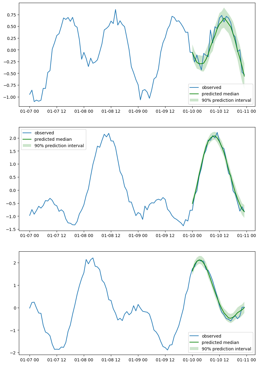
Train and visualize forecasts

Let’s generate 100 time series dataframes, create a train/test split, train an estimator and visualize the forecasts.

prediction_length, freq = 24, "1H"
T = 10 * prediction_length
date_range = pd.date_range("2021-01-01", periods=T, freq=freq)

N = 100
time_seriess = [generate_single_ts(date_range, item_id=i) for i in range(N)]

train = PandasDataset([ts.iloc[:-prediction_length, :] for ts in time_seriess])
test = PandasDataset(time_seriess)

estimator = DeepAREstimator(
    freq=freq,
    prediction_length=prediction_length,
    trainer=Trainer(epochs=10),
)
predictor = estimator.train(train)
forecast_it, ts_it = make_evaluation_predictions(dataset=test, predictor=predictor)
forecasts = list(forecast_it)
tests = list(ts_it)
evaluator = Evaluator(quantiles=(np.arange(20) / 20.0)[1:])
agg_metrics, item_metrics = evaluator(tests, forecasts, num_series=len(test))

100%|██████████| 50/50 [00:03<00:00, 14.84it/s, epoch=1/10, avg_epoch_loss=0.621]
100%|██████████| 50/50 [00:03<00:00, 15.42it/s, epoch=2/10, avg_epoch_loss=-0.309]
100%|██████████| 50/50 [00:03<00:00, 15.52it/s, epoch=3/10, avg_epoch_loss=-0.417]
100%|██████████| 50/50 [00:03<00:00, 14.90it/s, epoch=4/10, avg_epoch_loss=-0.475]
100%|██████████| 50/50 [00:03<00:00, 15.25it/s, epoch=5/10, avg_epoch_loss=-0.503]
100%|██████████| 50/50 [00:03<00:00, 15.48it/s, epoch=6/10, avg_epoch_loss=-0.532]
100%|██████████| 50/50 [00:03<00:00, 15.48it/s, epoch=7/10, avg_epoch_loss=-0.558]
100%|██████████| 50/50 [00:03<00:00, 15.34it/s, epoch=8/10, avg_epoch_loss=-0.57]
100%|██████████| 50/50 [00:03<00:00, 15.34it/s, epoch=9/10, avg_epoch_loss=-0.591]
100%|██████████| 50/50 [00:03<00:00, 15.70it/s, epoch=10/10, avg_epoch_loss=-0.592]
Running evaluation: 100%|██████████| 100/100 [00:00<00:00, 1964.53it/s]

Let’s plot a few randomly chosen series.

n_plot = 3
indices = np.random.choice(np.arange(0, N), size=n_plot, replace=False)
fig, axes = plt.subplots(n_plot, 1, figsize=(10, n_plot * 5))
for index, ax in zip(indices, axes):
    ax.plot(tests[index][-4 * prediction_length :].to_timestamp())
    plt.sca(ax)
    forecasts[index].plot(intervals=(0.9,), color="g")
    plt.legend(["observed", "predicted median", "90% prediction interval"])