Abstract
Printed phantoms hold great potential as a tool for examining task-based image quality of x-ray imaging systems. Their ability to produce complex shapes rendered in materials with adjustable attenuation coefficients allows a new level of flexibility in the design of tasks for the evaluation of physical imaging systems. We investigate performance in a fine “boundary discrimination” task in which fine features at the margin of a clearly visible “lesion” are used to classify the lesion as malignant or benign. These tasks are appealing because of their relevance to clinical tasks, and because they typically emphasize higher spatial frequencies relative to more common lesion detection tasks.
A 3D printed phantom containing cylindrical shells of varying thickness was used to generate lesions profiles that differed in their edge profiles. This was intended to approximate lesions with indistinct margins that are clinically associated with malignancy. Wall thickness in the phantom ranged from 0.4mm to 0.8mm, which allows for task difficulty to be varied by choosing different thicknesses to represent malignant and benign lesions. The phantom was immersed in a tub filled with water and potassium phosphate to approximate the attenuating background, and imaged repeatedly on a benchtop cone-beam CT scanner.
After preparing the image data (reconstruction, ROI Selection, sub-pixel registration), we find that the mean frequency of the lesion profile is 0.11 cyc/mm. The mean frequency of the lesion-difference profile, representative of the discrimination task, is approximately 6 times larger. Model observers show appropriate dose performance in these tasks as well.
Keywords: Physical Phantoms, 3D Printing, Image-Quality Assessment
1. INTRODUCTION
Many tasks in medical imaging involve classifying a visible lesion as malignant or benign1–3. It is often the case the features of the lesion boundary are critical to such tasks. In particular, the appearance of an indistinct region at the edge of a lesion can be indicative of invasive growth that is associated with many forms or malignant disease4,5. From the perspective of task-based assessment of image quality, such boundary discrimination tasks should serve as endpoints for imaging system optimization6–8.
In this work we investigate boundary discrimination tasks using a novel 3D printed phantom that utilizes the thickness of cylindrical printed walls to represent the presence or absence of locally invasive growth. Discriminating lesions with a thick wall (malignant) from those with a thin wall (benign) focuses on the ability of the imaging system to accurately render the boundary of a lesion without excessive amplification of noise. We show that these tasks emphasize higher spatial frequencies than a more conventional lesion detection task and we evaluate the performance of model observers in discriminating phantom “lesions” with different wall thicknesses.
2. METHODS
The evaluation of cancerous lesions often involves an assessment of a lesion’s boundary (or margin). In some cases, invasive cells will produce an indistinct or irregular edge that serve as an important diagnostic feature9. The phantom used here attempts to approximate the appearance of a lesion by a circular region of high intensity as a model of a lesion, and a lower contrast ring around lesion with a wall thickness that models the appearance of potentially malignant cells. In this somewhat stylized scenario, a thicker wall indicates greater malignant potential. We describe the construction of a printed physical phantom for this purpose, how it was imaged in a laboratory setting, and how the images were analyzed to show signal and noise profiles as well as model-observer performance assessments.
2.1. Description of the Phantom
A 3D phantom was designed and printed from resin that cures to a measured attenuation coefficient of 0.0247 cm−1. We used an Elegoo Mars LCD printer (Shenzhen, China) and a water-washable photopolymer resin. The shape of the phantom was a series of 8 cylinders with varying wall thicknesses of 0.4mm, 0.6mm, 0.7mm, and 0.8mm (2 cylinders at each wall thickness) all connected by a base of approximately 1cm thickness. Tube wall thickness was confirmed using a digital caliper, with +/− 0.02 mm tolerance. The diameter of each cylinder was adjusted so that the midpoint of the cylinder wall was at a diameter of 5.8mm. This gave all the lesions approximately the same total integrated intensity.
Each cylinder was filled with water containing dissolved potassium phosphate such that the attenuation coefficient insider the cylinder was 0.0270 cm−1. The cylinder phantom was then immersed in a background of water containing dissolved potassium phosphate so that the attenuation coefficient was 0.0224 cm−1. Figure 1A shows a photograph of the printed phantom just before imaging.
Figure 1. Printed Cylinder phantom and Images.

The phantom itself (A) consists of printed cylinders immersed in water mixed with calcium phosphate to achieve specific levels of attenuation (see text). The trans-axial reconstructed image (B) shows the position of simulated lesions with differing wall thicknesses representing more or less distinct boundaries. The axial slice (C) shows the z-range of the 3D images used to generate 2D ROIs (201 slices).
2.2. Imaging of the phantom
The phantom was imaged using a benchtop cone-beam CT system at 3 exposure levels (50, 100, and 300 mAs), with 10 repeated scans at each dose. The x-ray source was a Varex Rad-94 (Salt Lake City, UT) operated at 80kVp, and the flat-panel detector was a Varex 4343CB (Salt Lake City, UT) with a detector pixel size of 0.278 mm. The SDD and SAD were 1000.5mm and 499.7 respectively, resulting in a magnification factor of approximately 2. The phantom was rotated and scanned over 360° (1° increments) using a Physik Instrumente (Auburn, MA) rotary table. The images were reconstructed using filtered back-projection with Hamming-window apodization on an isotropic voxel grid with 0.139mm spacing between samples. A vertical range of 201 slices was found to be acceptable in terms of imaging uniformity, as shown in Figure 1B. The lateral position of the 8 cylindrical lesions within the phantom with labeled wall thicknesses is shown in Figure 1C.
To simplify the subsequent analysis and facilitate the use of these images for analysis and performance assessments, we extracted 2D ROIs centered on each lesion. Imperfections in the printing and positioning of the phantom gave the cylinders a slight tilt angle relative to the voxel sampling. To account for this, a subpixel registration algorithm was used to center each lesion in a small ROI (1092 pixels and 15.15 mm2) on the pixel that was closest to the lesion center. Additionally, preliminary analyses showed that the background intensity differed across the lesions. In discrimination tasks using different lesions, this intensity difference can be used by model observers (or potentially human observers as well) to identify the lesion, effectively making the background difference equivalent to “signal”. To normalize for different background intensities, we subtracted a small constant term from each lesion ROI so that the average intensity of all the ROIs for a given lesion was constant across lesions.
This resulted in a total of 4020 ROIs for each wall thickness at each dose level imaged. Figure 2A shows sample ROI images at each dose level and for the thinnest- and thickest-walled lesions. Figure 2B shows the average ROI image for each lesion, which allows the halo around the central portion of the lesion to be more clearly visualized. The tasks used here involve discriminating an ROI from the 0.4mm wall thickness from one of the others, and so we expect increasing performance going from 0.6mm to 0.8mm.
Figure 2. ROI images.
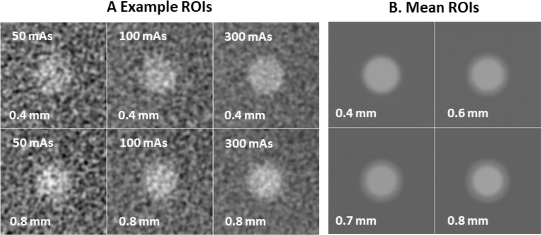
Example ROI images (A) of the 0.4mm wall-thickness (top row) and the 0.8mm lesion (bottom row) at the 3 dose levels used show the appearance and texture of noise in the ROI images and some sense of the faint halo around the “invasive” (0.8mm) lesion. The mean ROI stimulus (B) for each wall thickness is shown indicating the increasing low-attenuation rim surrounding the bright central region.
2.3. Mean Frequency of the Task
We are also interested in the spectral content of these tasks, which we quantify in terms of the mean frequency. Let for represent the average ROI shown in Figure 2B, with for a wall thickness of 0.4mm to for a wall thickness of 0.8mm, and let for be the difference signal for the three tasks considered in this work. We define as the 2D FFT of the difference signal, and frequency radius of the point [k,l], given by , where
and with a similar definition for vl. The mean frequency is then defined as the ratio
| (1.1) |
For comparison, we would like to know the mean frequency of the lesion itself, which we define as the 0.4 mm wall thickness profile with the mean background subtracted, . The mean frequency of the lesion is computed in a similar fashion to Eq. (1.1), but with , the 2D FFT of L[n,m], instead of .
2.4. Noise Power Spectrum (NPS)
The average images shown in Figure 2B contain effects of the system transfer function manifest as a slight blurring of edges in the image. In addition to transfer effects, noise properties of the ROIs are also an important characterization of the images. We compute the noise-power spectrum of the ROIs for this purpose.
An NPS is computed for each mAs setting, lesion, and depth by a sample average over the 10 replicated images. These are averaged over depth and lesion into one 2D NPS for each mAs setting. To control for spectral leakage, a tapered window is used that is constant out to a radius of 27 pixels, and then rolls off to zero at 54 pixels with a cosine profile. The resulting noise-power spectra are shown in Figure 3 as plots in radial frequency. These plots show that the images are somewhat oversampled given that the apodization filters implemented in the reconstruction process drive the spectra to zero by even though the Nyquist frequency for the pixel size is .
Figure 3. ROI Noise Power Spectra.
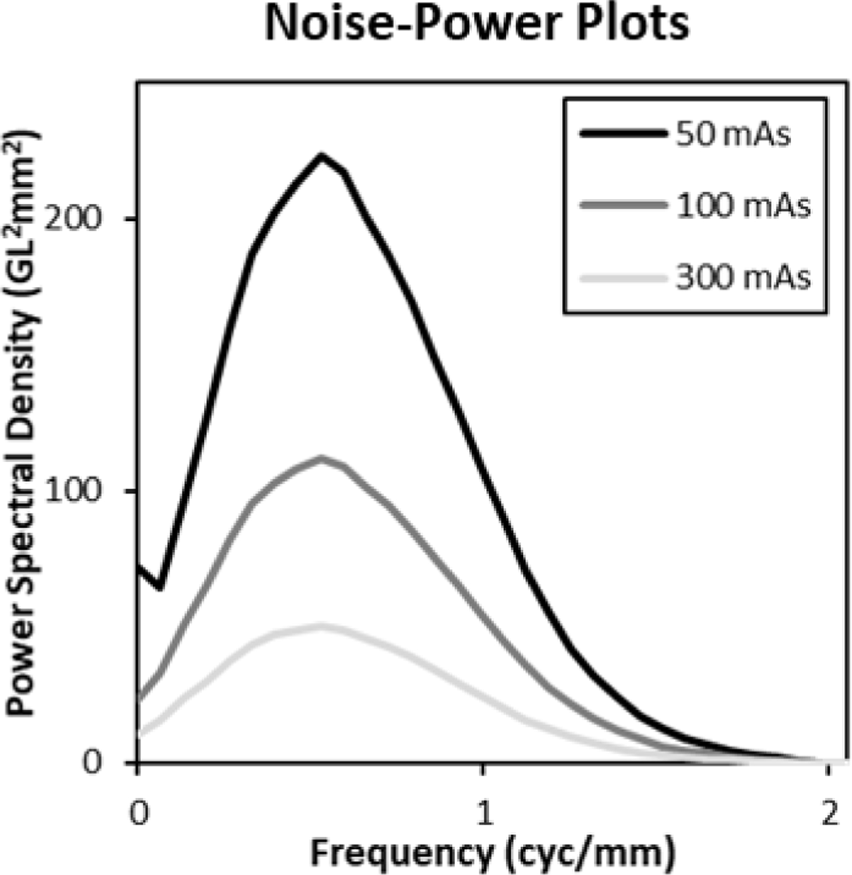
Noise power spectra for each mAs setting (averaged over lesion and depth) are shown. The spectra rise at low frequencies with a characteristic ramp, and then fall back to zero because of noise apodization implemented in the reconstruction process.
2.5. Model Observers
We will investigate the performance of two model observers in this work, a non-prewhitening matched filter (NPWMF) and a prewhitening matched filter (PWMF). Additionally, we will evaluate the performance of these models using two different computational approaches that are described here. Differences in performance between these two methods indicate potential violations of assumptions in the modeling of observer performance.
2.5.A. Model-Observer Performance Measures.
The NPWMF and PWMF have a long history of use in image quality evaluation10–13. The models are defined by a template, , that is used to generate a decision variable from a sample image, , via an inner product
| (1.2) |
The templates for the NPWMF and PWMF models is described in more detail in the next section. If we imagine responses from a sample of malignant images, for , and samples from benign images , then we can estimate the forced-choice proportion correct as
| (1.3) |
where the Step function is 0 for negative argument, 1 for positive arguments, and 1/2 for an argument of 0. It is well known that PC is equivalent to the area under the empirical ROC curve (AUC) as well14,15.
The proportion correct/AUC in Eq. (1.3) represents achievable performance, since it is derived from actually performing the task of interest. However, we can use equivalent measures under assumptions involving the statistical properties of the images. For example, if we are discriminating lesion from lesion 0 , we can estimate the mean image in each class from the average lesions shown in Figure 2B. If we can further assume that the noise in the ROIs is approximately Gaussian and characterized by the power spectra in Figure 3, then we can define the template detectability index for this task, , as
| (1.4) |
where is the standard deviation of the template responses for noise defined by the x-ray tube current (A). This can be computed by taking the 2D FFT of w, multipling by the 2D NPS, inverse transforming, taking the inner product of the resulting image with w, and finally taking the square root of this quantity. The detectability index is converted to PC by the relation
| (1.5) |
When across multiple conditions, then it may be assumed that the responses are approximately Gaussian and determined by the conditional means and power spectra.
2.5.B. Model-Observer Templates.
The non-prewhitening matched filter (NPWMF) model is defined by the use of the difference signal as a linear template for discrimination of malignant from benign ROIs. The pre-whitened matched filter model (PWMF) also uses the difference signal, but it filters this signal by the inverse of the NPS. As seen in Figure 3, the NPS is dropping to zero near 2 cyc/mm, which makes a simple division by the NPS unstable. Two modifications to the basic formula for the WMF are implemented to counteract this instability: A small positive constant is added to the NPS before inversion, and the resulting spectrum is rolled off to zero with a cosine profile from to .
Images of a NPWMF and PWMF template are shown in Figure 4A for the discrimination of the 0.8mm wall-thickness lesion from the base 0.4mm wall-thickness lesion. The bright region of the outsize results from the “halo” of low intensity wall in the 0.8mm lesion. The dark region inside this is due to the difference between the wall in the 0.8mm lesion and the interior of the 0.4mm lesion. The PWMF template shows somewhat more variability that is likely due to estimation error in the NPS used to define it. The spectral plots shown in Figure 4B show the oscillation expected from a signal that is predominantly in a spatial ring around the origin. The plots show that the effect of discriminating a thicker wall is predominantly an amplification of the spectral amplitude, except near the origin. These is some evidence of relatively suppressed amplitudes in the PWMF at frequencies near , where the NPS in Figure 3 peaks, as well as extension further into the frequency domain than for the NPWMF.
Figure 4. NPWMF and PWMF Templates.
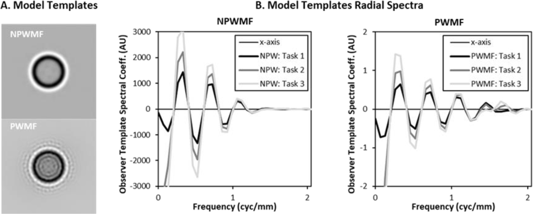
The 2D images of the observer templates (A), for the 0.8mm vs 0.4mm wall-thickness discrimination task, show the emphasis on signals at the boundary of the lesion. The PWMF shows somewhat more radial oscillation. The radial frequency plots (B) show the oscillation of the frequency components. The plots show the spectra for all three tasks (0.8mm, 0.7mm, and 0.6mm wall thickness vs 0.4mm wall thickness), which are manifest predominantly as increased amplitude.
3. RESULTS AND DISCUSSION
3.1. Task Mean Frequency
One of the focuses of this work is a demonstration that discrimination tasks can be useful for demonstrating the benefits of higher resolution imaging systems, since they rely on high frequencies for task performance. Figure 5A shows the base lesion profile, a 5mm diameter disk in the 2D ROI, as well as the difference signal between lesions with 0.6mm wall thickness and a 0.4mm wall thickness. The lesion profile would be a typical signal used in a lesion detection task, whereas the difference signal is the relevant profile for the boundary discrimination task investigated here.
Figure 5. Lesion and Difference Signal.
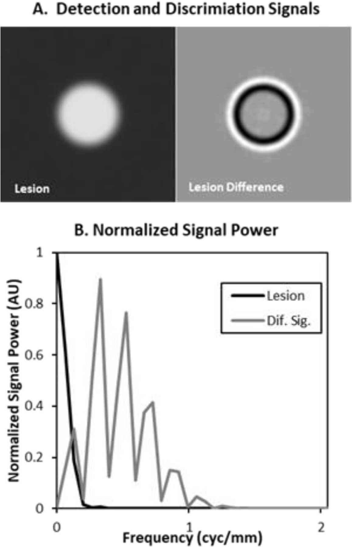
The images (A) show the base lesion used in these studies as well as the difference between lesions with 0.4mm and 0.6mm wall thicknesses. Plots of the normalized radial spectral power of these signals show that the lesion is concentrated at very low frequencies (< 0.2cyc/mm), while the difference signal extends past 1cyc/mm.
The normalized spectral power (normalized by the maximum spectral power) plotted in Figure 5B shows that the difference signal has spectral content at much higher frequencies than the lesion. This is reflected in the mean frequency computed as in Eq (1.1). The mean frequency of the lesion is 0.11cyc/mm while the mean frequency of the difference signal is 0.59 cyc/mm, nearly 6 times larger.
3.2. Model Observer Performance
Performance for discriminating the 3 thicker walled lesions from the 0.4mm lesion was evaluated for the non-prewhitened matched filter (NPWMF) and the prewhitened matched filter (PWMF) for all three levels of mAs. The PWMF also required the estimated the NPS profiles shown in Figure 3 to achieve the prewhitening step described in Section 2.5.B.
We computed PC/AUC performance for the two methods described in Eq.s (1.3) and (1.5). The results are shown in Figure 6. For the computation from samples (Eq. (1.3)) in Figure 6A, performance results are consistent with what we would expect. Performance increases as the wall thickness of the malignant lesion increases, as the dose increases, and also going from the NPWMF to the PWMF model observer. These effects are aslo seen for the statistical performance computation shown in 6B. However, there is a substantial boost in performance going from the sample estimates of performance to the statistical estimates, and this suggests that there are still some anomalous imaging effects that are unaccounted for.
Figure 6. Discrimination Performance.
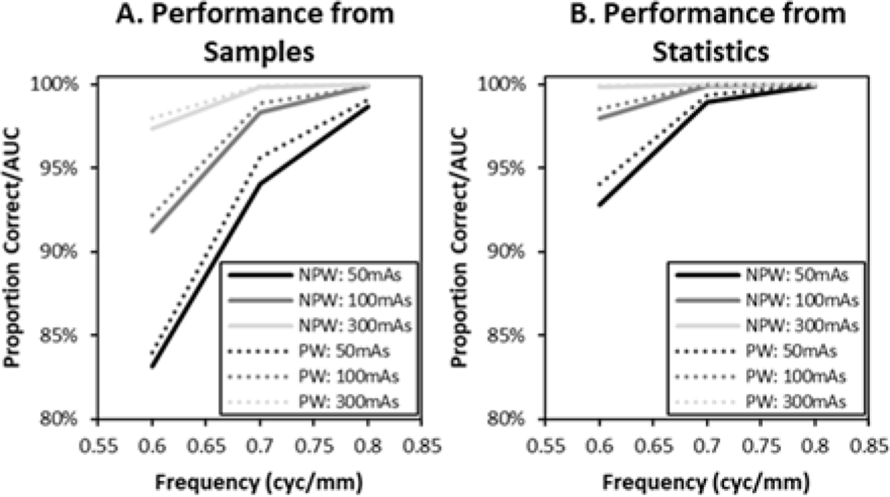
Performance (PC/AUC) estimates based on model observer responses to sample images (A) show performance effects from malignant-lesion wall thickness, dose, and the model observer used to evaluate performance. Performance from statistical properties (B) shows similar effects, but an overall elevated level of performance.
We would argue that this performance mismatch illustrates the usefulness of physical phantom images for evaluating performance. The imaging process is a complex cascade of events that involve many physical processes and components. Summary statistics like a transfer function or a noise power spectrum are necessary for characterizing performance of these systems, but not necessarily sufficient. A physical phantom allows all the components of the imaging process to affect the final images.
4. SUMMARY AND CONCLUSIONS
The purpose of this work has been to report initial imaging results using a novel printed phantom that creates “lesions” with fine features for discrimination tasks. These tasks make substantially greater use of high spatial frequencies relative to more common lesion detection tasks, and hence they may be of value for assessment of high resolution imaging systems. We find that initial performance results for non-prewhitening and prewhitening matched-filter models exhibit performance effects that are consistent with what we would expect, with improvements for an easier task (greater wall-thickness), less noise (mAs), or a better “observer” (PWMF vs NPWMF). However, it is also clear that the method used for performance evaluation can have a large effect on overall performance. We take this as a fundamental demonstration of the importance of imaging with a physical phantom.
Acknowledgments
This work was supported by the NIH through research grant (R01-EB025829). The content of this proceedings paper is solely the responsibility of the authors and does not represent the institutional views of any funding agency.
REFERENCES
- 1.Hadjiiski L, et al. Improvement in radiologists’ characterization of malignant and benign breast masses on serial mammograms with computer-aided diagnosis: an ROC study. Radiology 233, 255–265 (2004). [DOI] [PubMed] [Google Scholar]
- 2.Johnson JP, et al. Using a visual discrimination model for the detection of compression artifacts in virtual pathology images. IEEE Trans Med Imaging 30, 306–314 (2010). [DOI] [PMC free article] [PubMed] [Google Scholar]
- 3.Richard S & Siewerdsen JH Comparison of model and human observer performance for detection and discrimination tasks using dual‐energy x‐ray images. Medical Physics 35, 5043–5053 (2008). [DOI] [PMC free article] [PubMed] [Google Scholar]
- 4.Sato H, et al. A matrix metalloproteinase expressed on the surface of invasive tumour cells. Nature 370, 61–65 (1994). [DOI] [PubMed] [Google Scholar]
- 5.Boccaccio C & Comoglio PM Invasive growth: a MET-driven genetic programme for cancer and stem cells. Nature Reviews Cancer 6, 637–645 (2006). [DOI] [PubMed] [Google Scholar]
- 6.Burgess A, Jacobson F & Judy P Mass discrimination in mammography: experiments using hybrid images1. Academic radiology 10, 1247–1256 (2003). [DOI] [PubMed] [Google Scholar]
- 7.Abbey CK, Zemp RJ, Liu J, Lindfors KK & Insana MF Observer efficiency in discrimination tasks simulating malignant and benign breast lesions imaged with ultrasound. IEEE Trans Med Imaging 25, 198–209 (2006). [DOI] [PMC free article] [PubMed] [Google Scholar]
- 8.Abbey CK, et al. Human observer templates for lesion discrimination tasks. in Medical Imaging 2020: Image Perception, Observer Performance, and Technology Assessment, Vol. 11316 113160U (International Society for Optics and Photonics, 2020). [DOI] [PMC free article] [PubMed] [Google Scholar]
- 9.Tamaki K, et al. Correlation between mammographic findings and corresponding histopathology: potential predictors for biological characteristics of breast diseases. Cancer Science 102, 2179–2185 (2011). [DOI] [PubMed] [Google Scholar]
- 10.Myers KJ, Barrett HH, Borgstrom MC, Patton DD & Seeley GW Effect of noise correlation on detectability of disk signals in medical imaging. J Opt Soc Am A 2, 1752–1759 (1985). [DOI] [PubMed] [Google Scholar]
- 11.Wagner RF & Brown GG Unified SNR analysis of medical imaging systems. Phys. Med. Biol 30, 489–518 (1985). [DOI] [PMC free article] [PubMed] [Google Scholar]
- 12.Barrett HH, Yao J, Rolland JP & Myers KJ Model observers for assessment of image quality. Proc Natl Acad Sci U S A 90, 9758–9765 (1993). [DOI] [PMC free article] [PubMed] [Google Scholar]
- 13.Burgess AE Statistically defined backgrounds: performance of a modified nonprewhitening observer model. J Opt Soc Am A Opt Image Sci Vis 11, 1237–1242 (1994). [DOI] [PubMed] [Google Scholar]
- 14.Green DM & Swets JA Signal detection theory and psychophysics, (Wiley, New York, 1966). [Google Scholar]
- 15.Metz CE Basic principles of ROC analysis. Semin Nucl Med 8, 283–298 (1978). [DOI] [PubMed] [Google Scholar]


